Water Resources of the Black Sea Catchment under Future Climate and Landuse Change Projections


1
Eawag, Swiss Federal Institute of Aquatic Science and Technology, 8600 Duebendorf, Switzerland
2
Department of Environmental Systems Science, ETH Zurich, 8092 Zürich, Switzerland
3
Laboratory of Hydrology and Water Management, Ghent University, 9000 Ghent, Belgium
4
Institute for Environmental Sciences, University of Geneva, 1227 Geneva, Switzerland
*
Author to whom correspondence should be addressed.
Water 2017, 9(8), 598; https://doi.org/10.3390/w9080598
Submission received: 11 April 2017
/
Revised: 13 July 2017
/
Accepted: 6 August 2017
/
Published: 12 August 2017
(This article belongs to the Special Issue Integrated Soil and Water Management: Selected Papers from 2016 International SWAT Conference)
Abstract
:As water resources become further stressed due to increasing levels of societal demand, understanding the effect of climate and landuse change on various components of the water cycle is of strategic importance. In this study we used a previously developed hydrologic model of the Black Sea Catchment (BSC) to assess the impact of potential climate and landuse changes on the fresh water availability. The BSC model was built, calibrated, and validated against observed daily river discharge for the period of 1973–2006 using the Soil and Water Assessment Tool (SWAT) as the modeling tool. We employed the A2 and B2 scenarios of 2017–2050 generated by the Danish Regional Climate Model (HIRHAM), and four potential future landuse scenarios based on the Intergovernmental Panel of Climate Change (IPCC)’s special report on emissions scenarios (SRES) storylines, to analyze the impact of climate change and landuse change on the water resources of the BSC. The detailed modeling and the ensemble of the scenarios showed that a substantial part of the catchment will likely experience a decrease in freshwater resources by 30 to 50%.
1. Introduction
Observational evidence from all continents and oceans shows that natural systems are affected by regional climate changes, particularly by increases in temperature [1]. Nearly all regions of the world are expected to experience a net negative impact of climate change on water resources and freshwater ecosystems [1]. A number of studies have shown that climate change will have significant effects on water availability, water stresses, and water demand [2,3]. Climate change will pose added challenges to managing high disaster-risk areas, as it is virtually certain that the frequency and magnitude of warm daily temperature extremes will increase, and cold extremes will decrease, in the 21st century at the global scale [1]. It is expected that the frequency of heavy precipitation will increase in Southern and Central Europe and the Mediterranean region, and that droughts will intensify because of reduced precipitation and/or increased evapotranspiration [1].
The focus of this study is on the Black Sea Catchment (BSC), which lies in a transition zone between the Mediterranean region in an arid climate of North Africa and the temperate and rainy climate of central Europe. It is affected by interactions between mid-latitude and tropical processes. Because of these features, even relatively minor modifications of the general circulation can lead to substantial changes in the Mediterranean climate [4]. This makes the BSC a potentially vulnerable region to climatic changes as induced, for example, by increasing concentrations of greenhouse gases [4]. Indeed, the Mediterranean region has shown large climate shifts in the past, and it has been identified as one of the most prominent “Hot-Spots” in future climate change projections [5].
For the long-term strategic planning of a country’s water resources in the face of the evolving climate and landuse changes, it is important to quantify the effects with a high spatial and temporal resolution. However, no publication has really focused on the long-term evaluation of the BSC’s water balance under a combination of climate and landuse change. Yet this may be the most beneficial application of hydro-climatology to support long-term water resources management and planning. Within this context, Giorgi and Lionello [4] reviewed a few climate change projections over the Mediterranean region based on the most recent and comprehensive ensembles of global and regional climate change simulations. There is also a comprehensive review of climate change projections over the Mediterranean region reported by Ulbrich et al. [6] based on a limited number of global and regional model simulations performed throughout the early 2000s. Moreover, a number of studies have reported regional climate change simulations over Europe, which includes parts of the BSC [7,8,9,10]. As recognized by the two international environmental organizations in the region (Danube and Black Sea), achieving an environmental sustainability that will improve human well-being strongly depends on sustainable water resources management in this catchment [11]. Nevertheless, despite the importance of this region within the global change context, assessments of water resources of the entire catchment under different climate and landuse change projections do not exist in the literature.
Hydrologic models often used to assess the impacts of land and climate changes on water resources include: WaterGap3 [12,13], HBV [14], MIKE-SHE [15], and the Soil and Water Assessment Tool (SWAT) [16] among many others. These models are particularly useful as they can assess past as well as possible future impact scenarios. SWAT [16] has proven its suitability for hydrologic impact studies, especially under conditions of limited data availability [17]. The aforementioned hydrological models often use global climate simulations for the 20th and 21st century under different greenhouse gas forcing scenarios that are publicly available as a contribution to the fourth and fifth Assessment Reports (AR4, AR5) of the Intergovernmental Panel on Climate Change (IPCC) to analyze the climate change impacts on various aspect of hydrological cycle. In the current study, we employed the Danish Regional Climate Model (RCM) HIRHAM, driven by the United Kingdom’s Hadley Center HadAM3H Global Climate Model (GCM), under the scope of the PRUDENCE project to assess the future climate change projections over the BSC. We used the quantification of landuse change scenarios which is based on the framework provided by the Integrated Model to Assess the Global Environment (IMAGE) [18]. The four landuse change scenarios used in the current study comprise a number of plausible storylines based on the IPCC’s special report on emissions scenarios (SRES) following four marker scenarios representing different global socio-economic development pathways.
The objective of the study is to address the changes in various components of the water balance including precipitation, evapotranspiration, and soil moisture under changing climate and landuse. We used a previously calibrated hydrological SWAT model of the BSC [19] as the base model, and incorporated the climate and land use change scenarios that are outlined above. We assessed the variation in blue water (river discharge plus aquifer recharge) and green water (soil moisture and evapotranspiration) across the BSC under changing climate and landuse scenarios.
2. Material and Methods
2.1. Study Area
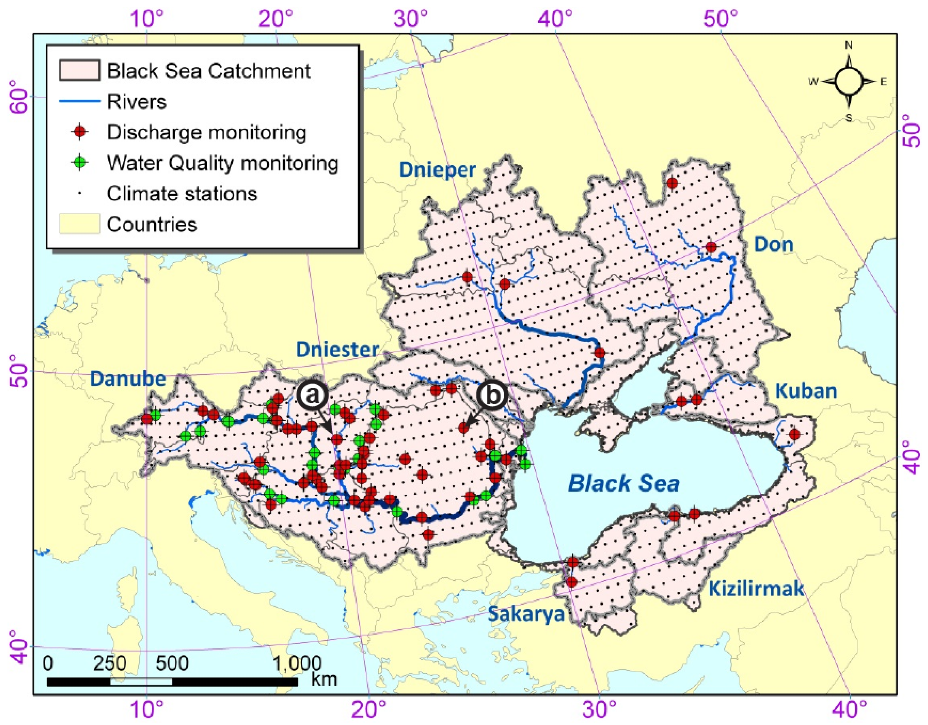
The BSC drains rivers of 23 European and Asian countries (Austria, Belarus, Bosnia, Bulgaria, Croatia, Czech Republic, Georgia, Germany, Hungary, Moldova, Montenegro, Romania, Russia, Serbia, Slovakia, Slovenia, Turkey, Ukraine, Italy, Switzerland, Poland, Albania, and Macedonia) from an area of 2.3 million km2 into the Black Sea (Figure 1). The catchment is highly populated (160 million people) [20]. Major rivers draining into the Black Sea include Danube, Dniester, Dnieper, Don, Kuban, Sakarya, and Kizirmak. The major mountainous peaks lie in the East and South, in the Caucasus and in Anatolia, and to the Northwest with the Carpathians in the Ukraine and Romania. Most of the rest of the West and North of the catchment is low lying. The catchment has a distinct North–South temperature gradient from <−3 °C to >15 °C (annual average) and a West–East precipitation gradient that is decreasing with distance from the Atlantic Ocean. Areas of high precipitation (>3000 mm year−1) are in the West, and areas of low precipitation (<190 mm year−1) are in the North and East [21]. The dominant landuse in the catchment is agricultural land, with 65% coverage according to MODIS Land Cover [22].
2.2. Soil Water Assessment Tool (SWAT)
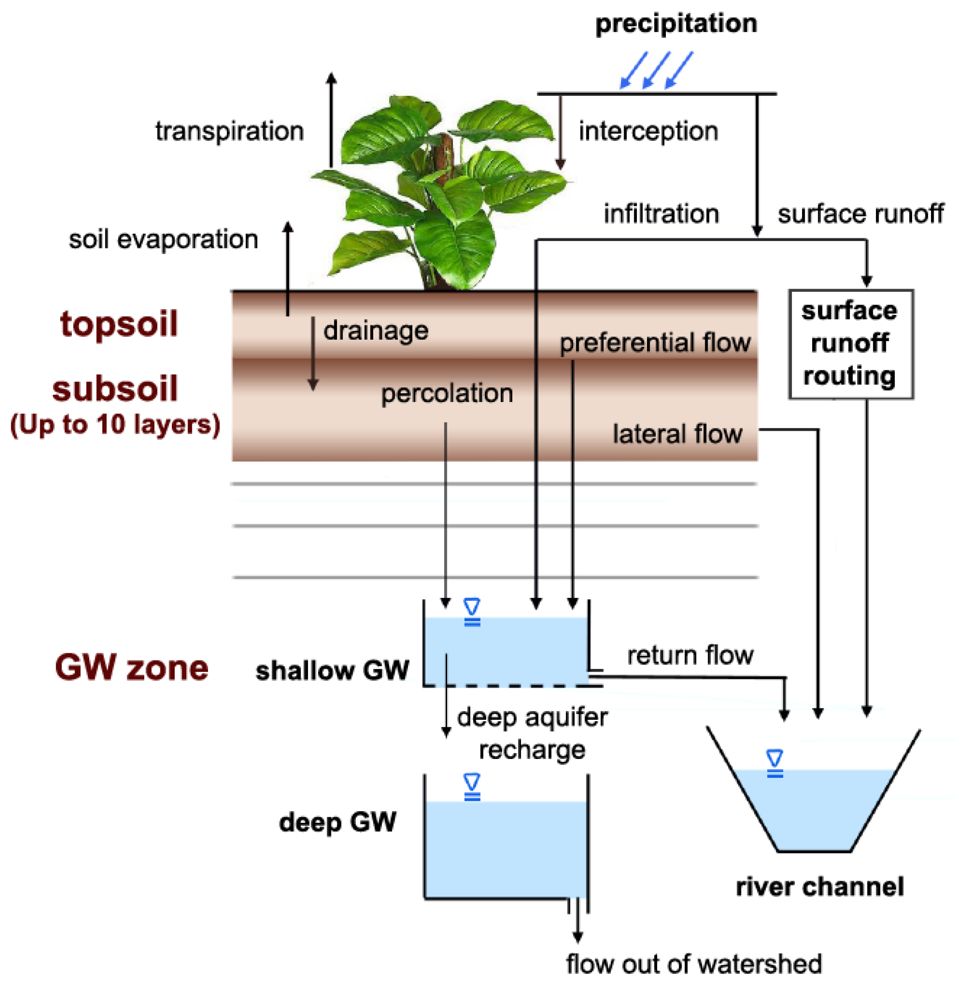
SWAT was used to simulate the hydrology of the BSC. SWAT is a process-based, semidistributed hydrologic model that is developed to quantify the impact of land management practices on water, sediment, and agricultural chemical yields in large complex watersheds with varying soils, landuses, and management conditions over long periods of time. SWAT has been used for the assessment of landuse and management impacts on water quantity and quality in many studies worldwide. The spatial heterogeneity of the watershed is preserved by topographically dividing the catchment into multiple sub-basins. The sub-basins are further subdivided into hydrologic response units (HRU). These are lumped areas within a sub-basin with a unique combination of slope, soil type, and landuse that enable the model to reflect differences in evapotranspiration for various crops and soils. A simulation of the hydrologic cycle is separated into a land phase and a water phase [23]. The simulation of the land phase is based on the water balance equation, which is calculated separately for each HRU. Runoff generated in the HRUs is summed up to calculate the amount of water reaching the main channel in each sub-basin [23]. The water phase of the hydrologic cycle describes the routing of runoff in the river channel, using the variable storage coefficient method by Williams [24]. A detailed description of the model can be obtained from Neitsch et al. [23]. Figure 2 depicts a schematic view of processes accounting for the land phase of the SWAT model.
2.3. Landuse Scenarios
The landuse scenarios that are used in the current study were developed within the European Union’s seventh research framework through the enviroGRIDS project [25]. The developed scenarios comprise a number of plausible storylines based on a coherent set of assumptions, key relationships, and driving forces, to create a set of quantitative, internally consistent, and spatially explicit scenarios of future landuse covering the entire BSC (Figure 3). A trend of landuse change for different scenarios is summarized in Table 1.
The quantification of landuse scenarios is based on the outputs of the Integrated Model to Assess the Global Environment [18] and on projections based on data from the Statistical Office of the European Communities (Eurostat) and the UN World Population and Urbanization Prospects [26]. The European regional projections (forest, grassland, urban and built up, and cropland) were disaggregated at the level of smaller administrative units (Nomenclature of Units for Territorial Statistics, level 2 (NUTS2)), and then used as input to the regional/local land allocation Metronamica model [27] for 214 regions in the BSC. The landuse change scenarios were quantified as yearly changes in landuses on 1 km × 1 km grid cells, in two time steps, 2025 and 2050, for four scenarios covering the entire BSC. The landuse scenarios were developed for cropland, grassland, forest, and urban areas for the BSC countries, while the input data were derived from the MODIS land cover datasets [22] for the years 2001 and 2008. A full description of the scenario developments and quantitative measures of changes in land cover classes is presented by Mancosu et al. [28].
2.4. Climate Change Scenarios
Two future climate scenarios, HS and HB, were simulated for the period of 2010 to 2050, representing the IPCC’s A2 and B2 scenarios, respectively. In this study, we used precipitation and minimum and maximum temperature data from the PRUDENCE website. The data were downscaled and bias corrected using the Delta method [29] based on Climate Research Unit (CRU) [30] data (1901–2006). The CRU time series data for the control period are perturbed with changes, allowing increase as a function of time. These changes are based on the parted differences of the monthly probability distribution function (PDF). The PDF is partitioned into deciles, and observed time series are gradually perturbed. The assumption behind the Delta method is that future model bias for both mean and variability will be the same as for present-day simulations. Detail on downscaling techniques and a bias correction procedure is available in a study by Gago Da Silva et al. [31].
2.5. Model Setup, Calibration, and Validation
The 2.3 million km2 area of the catchment is divided into 12,982 sub-basins. The sub-basins are further divided into unique combination of soil, landuse, and slope, and formed 89,202 Hydrological Response Units (HRUs). For a calibration and uncertainty analysis, we used the Sequential Uncertainty FItting program SUFI-2, which is a tool for sensitivity analysis, multi-site calibration, and uncertainty analysis. SUFI-2 is linked to SWAT in the SWAT-CUP software [32].
The inputs of the model are summarized in Table 2. The simulation period was 1970–2006, designating the first three years as a warm up period. We used the ArcSWAT2009 interface for the model setup and SWAT2009 Rev528 for a model run. Table 3 gives an overview of the relevant methods used in the model setup. More details of the hydrologic model’s structure, setup, and performance in the BSC can be found in Rouholahnejad et al. [19].
For future simulations (2017–2050, including 3 years of warm up period), the two climate change scenarios (HB and HS) were paired with the four landuse change scenarios (BS ALONE, BS COOL, BS COOP, and BS HOT), leading to eight combinations of climate-landuse scenarios, and applied as inputs to the calibrated hydrologic model of the catchment in eight separate model setups. In addition, two model setups were designed to look at climate change only, with static landuse. The latter models used MODIS landuse data of the historical hydrologic model as the static landuse. In the other eight combinations of landuse-climate scenarios, a dynamically updating algorithm updated the landuses yearly up to the end of the simulation period. A total of 10 different scenarios were therefore built and analyzed.
3. Results and Discussion
The BSC hydrologic model was calibrated (1973–1996) and validated (1997–2006) at 144 river discharge stations at daily time scales. The most sensitive parameters to discharge are as shown in Table 4. An example of the simulated and observed stream flow along with the predictive uncertainty band for the two labeled river discharge stations in Figure 1 are presented in Figure 4. These are two examples of calibrated discharge stations, one at the border of Hungary and Romania and one in Romania. We ran the model and calibration simulations at a daily time scale. However, given the scale of the watershed, the outputs were extracted at monthly time scales.
3.1. Temperature and Precipitation in a Changing Climate
The HB and HS long-term average temperature scenarios show a 1–2.4 °C temperature increase with a west to east gradient in the catchment. While the overall long-term pattern of increase in temperature is similar in the two scenarios, HS depicts a larger temperature increase and over larger areas (Figure 5g,h). The variation over time in future temperature scenarios (2020–2050) has almost the same pattern as the historic temporal variation (1973–2006) with some discrepancies in the Danube basin (Figure 5b,d,f).
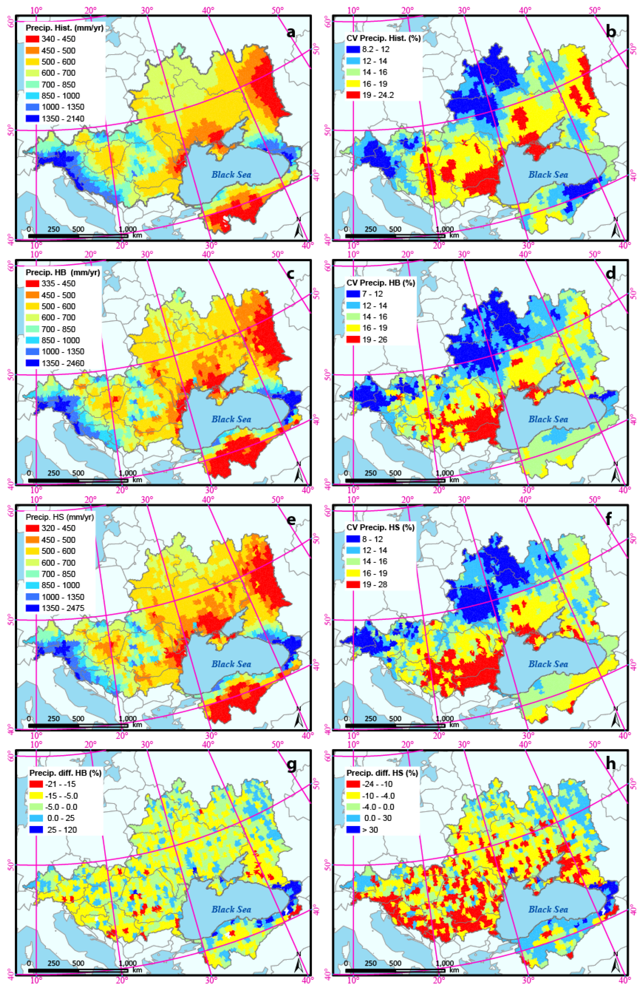
The historical distribution of average precipitation (Figure 6a), along with its coefficient of variation (CV) over time (Figure 6b), mark distinct precipitation distribution patterns with significant temporal variation (as indicated by the high CV values) in regions around the Sea, and in the Danube, Dnieper, and Don River basins. Historically, the upper Western part of the catchment in the alpine region receives rain of about 1300 mm year−1 on average, which is much higher than precipitation rates in other parts of the BSC where Ukraine, Russia, and Turkey lie. The regions with a smaller historical precipitation rates tend to show a higher temporal variation in precipitation (Figure 6b).
The two future precipitation scenarios are similar to the historic ones with regard to patterns of long-term annual averages (Figure 6a,c,e). In future scenarios, the areas with small precipitation expand as compared to the historic period (Figure 6a,c,e). The HS scenario, in general, suggests larger decreases in precipitation in the catchment.
The anomaly maps of precipitation (Figure 6g,h) depict percent deviation from historic precipitation for the entire catchment. The differences are calculated between the averages of 2020–2050 with those of 1973–2006. The HB scenario suggests a 5–15% decrease in precipitation in most regions of the catchment, while the HS suggests a 10–24% decrease in the precipitation of Danube Basin (West of the Black Sea) and a 4–10% decrease in precipitation in the rest of the catchment.
3.2. Fresh Water Resources under Changing Landuse and Climate
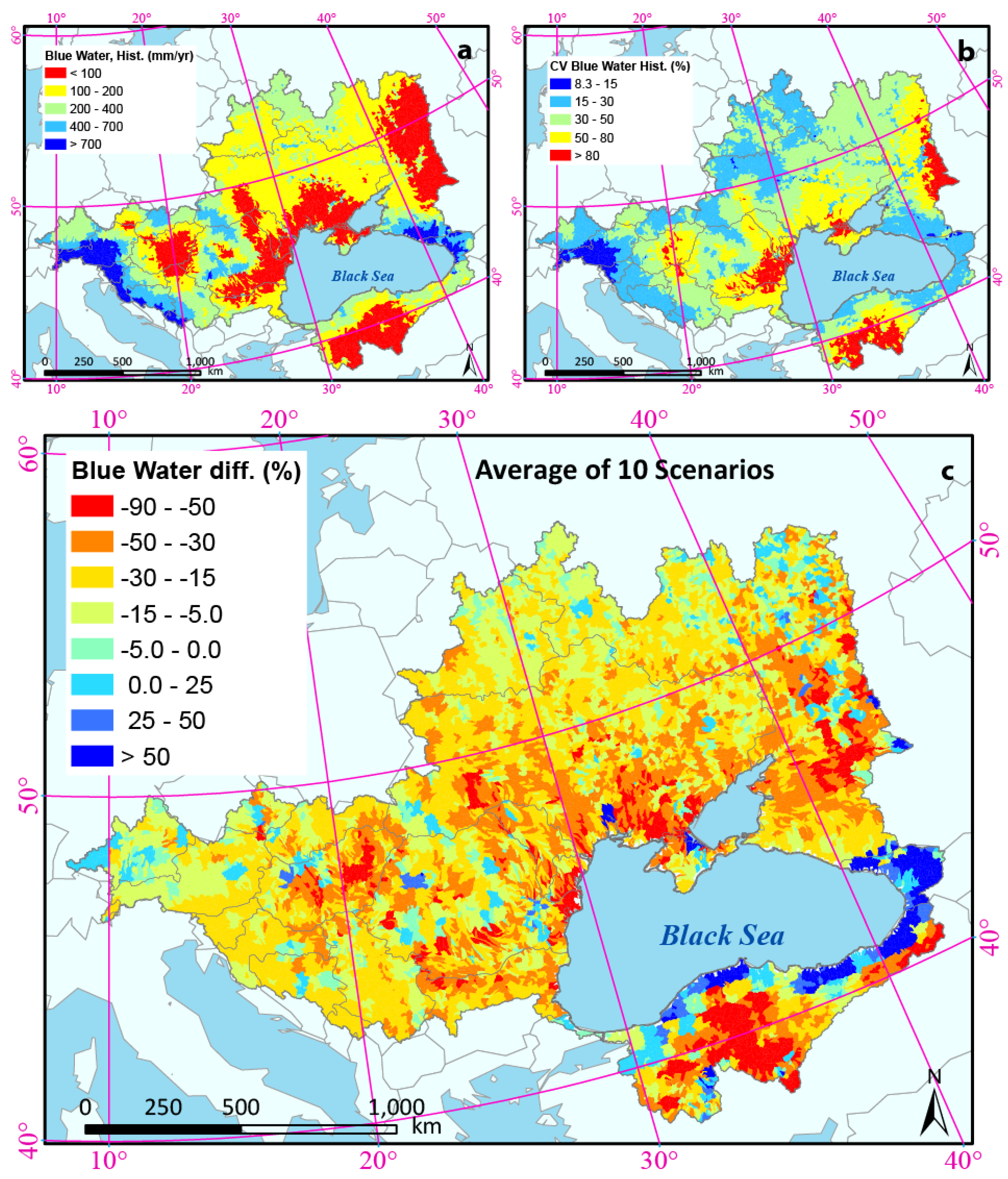
The term “blue water” [41] is widely used in the literature as the summation of the water yield and deep aquifer recharge. The long-term average blue water resources of the BSC for the period of 1973–2006 are shown in Figure 7a. The coefficient of variation of the blue water in the BSC (Figure 7b) during the period 1973–2006 shows significant variation in the central and eastern parts of the catchment as well as in Turkey, where the historic annual average of blue water is less than 100 mm year−1 (Figure 7b). In other words, the less the blue water is available, the more its variability over time is. The anomaly map of blue water (Figure 7c) depicts the deviation of long-term average blue water resources for the period of 2020–2050 from long-term average historic records (1973–2006) under future landuse and climate change scenarios (ensemble of 10 scenarios).
The blue water resources calculated with the ensemble of 10 scenarios suggest a 10–50% decrease in blue water resources in most parts of the catchment (Figure 7c). According to the future scenario ensembles, blue water increases on average by 50% in the coastal areas of Georgia and Turkey, with historically small blue water resources. However, this does not bring a significant increase in terms of net blue water resources availability of the whole catchment, as the historical records in these regions are quite small. Historical variations of blue water indicate low reliability (higher variability over time) of blue water resources in Romania, parts of Ukraine, the Russian parts of the catchment, and Turkey (Figure 7b). Our analysis shows that the poor conditions in these regions in terms of fresh water availability will be further intensified under climate change (Figure 7c).
As soil moisture is an integral component of rainfed agriculture, the soil water distributions projected under future climate change and landuse change scenarios are of a strategic importance. The spatial variation of long-term average annual green water storage (soil moisture) (Figure 8a) shows that most of the catchment lies in the range of 70–250 mm of soil moisture. However, the variation over time shows a distinct East–West pattern, suggesting different levels of reliability for soil water in the region. The Southern parts of the catchment tend to have smaller soil water with more variation over time (Figure 8b), which makes the region less reliable in terms of green water storage resources.
The anomaly map of soil water (average of 10 scenarios) depicts the deviation of average future (2020–2050) soil moisture from the average historic (1973–2006) soil moisture (Figure 8c). The average of the 10 scenarios shows up to a 10–25% reduction in soil water in the Danube catchment and Northern BSC in the upstream of Dnieper and Don, in Ukraine and Russia. There are indications of soil moisture increase in Georgia, where both climate scenarios suggested an increase in precipitation. The coefficient of variation among the 10 scenarios indicates that there is a good agreement between the scenarios with less than 2% variation in the prediction of soil water in most parts of the catchment and 10–15% variation in the Danube Delta and areas surrounding the Black Sea (Figure 8d).
The average of 10 scenarios suggests both an increase and a decrease in evapotranspiration across the BSC under climate and landuse change scenarios (Figure 9c). There is also a sharp increase in evapotranspiration of Georgia, which fits the increase in precipitation and temperature in this area. The variation among the 10 scenarios is the highest in the Danube delta and the Black Sea costal area. The average deviation from historic values (Figure 9c) suggests that evapotranspiration decreases by up to 12% in the Danube basin under future scenarios of change. The variation between model predictions of blue water, evapotranspiration, and soil moisture using four different future landuse scenarios shows limited impacts of landuse changes as compared to climate (the coefficient of variation is less than 1.3% among the four landuse scenarios) (Figure 10). Hence, the climatic signature is more significant than landuse in this study. The variations between scenarios are more pronounced in the blue water predictions (Figure 10a,b).
3.3. Extreme Events
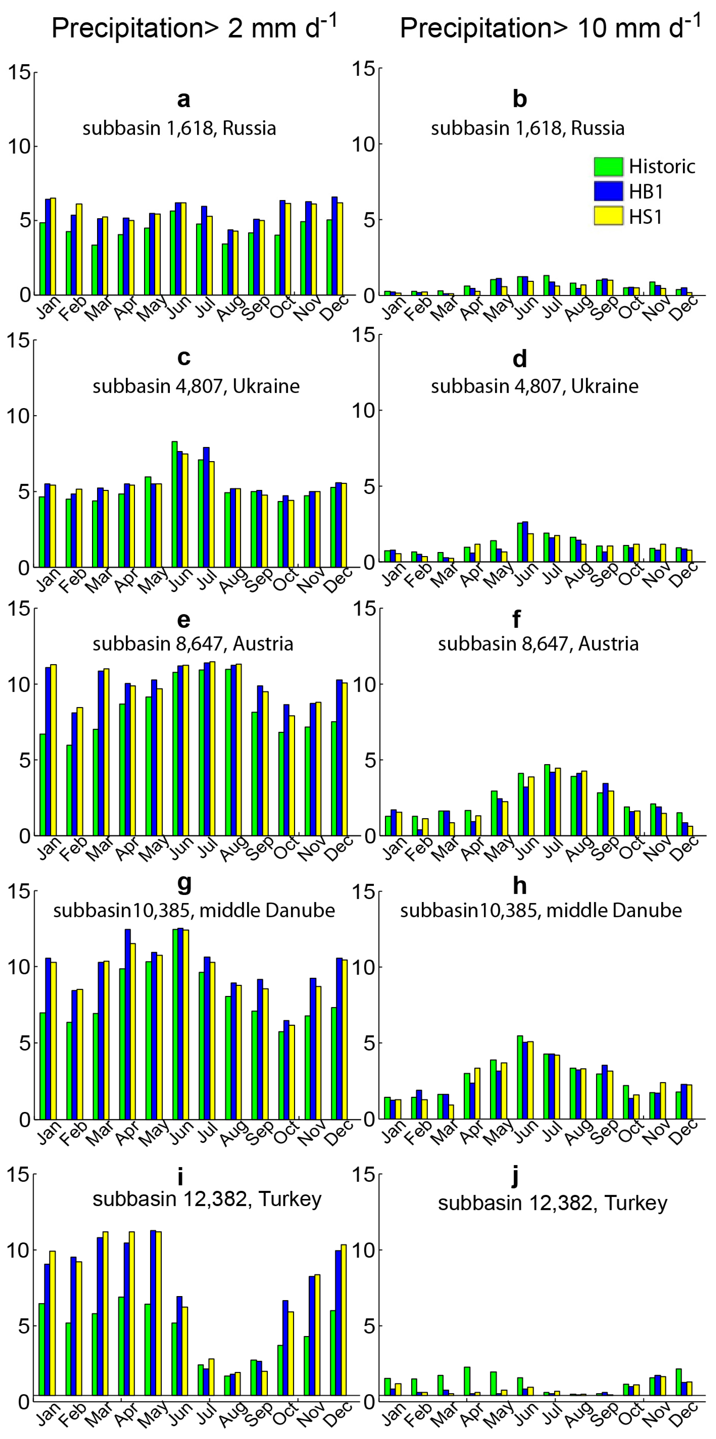
We compared the frequency of occurrences of wet days with the precipitation thresholds of >2 and >10 mm d−1 in five selected sub-basins in different climatic regions across the BSC (Figure 11). In general, although the long-term average precipitation based on the two scenarios suggests a general decrease in precipitation in the catchment, the frequency of the wet days are slightly higher under future scenarios. In a sub-basin in the Eastern part of the BSC in Russia, the two climate scenarios predicted a slightly higher number of days with precipitation larger than 2 mm as compared to historical climate (Figure 11a,b). This is a region with low annual rainfall (350–450 mm year−1) where there are few rainfall events exceeding 10 mm d−1 throughout the year. In a sub-basin in Southern Ukraine with 450–500 mm year−1 average annual precipitation, the frequency of wet days at the threshold of >2 mm d−1 stays as large as the historic period (Figure 11c). The slight decreases in number of days with >10 mm d−1 rainfall events indicate a smaller groundwater recharge, hence a larger chance of receding groundwater.
In the selected sub-basin in Austria with a rainfall rate of 1000–1350 mm year−1, the frequencies of wet days with more than 2 mm d−1 rainfall increase as compared with the historical data (Figure 11e).
In a sub-basin in the Alpine region in the middle of the Danube Basin, historic records of precipitation range between 1000–1350 mm year−1. Both the HB and HS scenarios predict an increase in the number of wet days with a threshold of >2 mm d−1, while the increase in the winter months is more distinct. The HS scenario predicts larger wet-day frequencies with the threshold of >10 mm d−1 than the HB scenario. The increase in precipitation frequencies at the threshold of >10 mm d−1 may indicate more flood risks in this region. However, the increase in the frequencies of precipitation with a large threshold (>10 mm d−1) stay within the historic records in this sub-basin (Figure 11h).
Finally, in a sub-basins in Turkey, the climate models behave differently from the Alpine region, as the HB and HS climate scenarios predict a distinctly larger number of days with precipitation more than 2 mm d−1 than what the historic records show. The precipitation events at 10 mm d−1 threshold, however, are predicted to decrease in this selected sub-basin in Turkey (Figure 11i,j).
4. Summary
Combinations of two regional climate scenarios and four regional landuse scenarios were incorporated in the current study to explore the possible future impacts of climate and landuse changes on water resources of the Black Sea Catchment. The landuse scenarios were driven by the IPCC’s special report on emissions scenarios (SRES) corresponding to four marker scenarios that represent different global socio-economic development pathways. The climate scenarios were generated from the Danish Regional Climate Model (RCM) (HIRHAM) for the IPCC’s SRES A2 and B2 scenarios (HS and HB scenarios respectively). On average, the climate scenarios suggested a 5–15% decrease in future long-term average annual precipitation in most parts of the catchment. The decrease in precipitation is more pronounced in the HS scenario. According to the HS climate scenario, the Western part of the catchment (Danube Basin) will experience a decline in precipitation by 25%. As the historic precipitation records are large in this region, this is expected to have a large impact on the water resources of the entire region, and leaves the catchment with a significant net decrease of precipitation. Both scenarios suggest an increase in temperature by up to 2 °C with a west to east gradient. The extent of changes in temperature is more severe in the HS scenario as compared to the HB scenario.
We also quantified the impacts of combined climate and landuse changes on freshwater distribution in the BSC. As suggested by the ensemble of scenarios, on average, the catchment is expected to experience a decrease in its blue water and green water storage resources, while the green water flow (evapotranspiration) increases in some parts of the catchment and decreases in other parts (Figure 7, Figure 8 and Figure 9). In addition, the decrease in fresh water resources in areas with high temporal variability in their water resources component (mainly in low lying countries around the Black Sea, such as Romania and Ukraine and the Russian part of the catchment) increases the vulnerability with regard to fresh water resources in these regions.
In our analysis, climate change had more pronounced effects on water resources, especially blue water, as opposed to the landuse change. To see the detailed effect of landuse change on the water resources component, it is beneficial to look at the water cycle at the HRU level, where the landuses are identical. This will give a true measure of landuse change impacts on water resources. The strength of the current work is the application of combined landuse and climate change scenarios. However, the study neglects the future changes in soil parameters over time, which accompanies changing landuses. Accounting for these changes will increase the confidence in the projected results, and needs to be further investigated.
An additional concern is the use of two regional climate scenarios (HS and HB) in model prediction while pursuing a thorough investigation based on the combined effect of many other Global Climate Models or Regional Climate Models would reflect climate model uncertainties, and hence is recommended. The study however, provides the basis to improve societal capabilities to anticipate and manage water resources both today and in the future climate change environment in the Black Sea Catchment.
Acknowledgments
This project has been funded by the European Commission’s Seventh Research Framework through the enviroGRIDS project (Grant Agreement n 226740). Elham Rouholahnejad Freund acknowledges funding from the Swiss National Science Foundation (SNSF grant P2EZP2_162279) during her stay at Ghent University. We are thankful to Emanuele Mancosu, Ana Gago Da Silva, and Saeid Ashraf Vaghefi for providing the landuse change and climate change scenarios. Special thanks to Raghavan Srinivasan for his instantaneous supports during the review process. The final manuscript benefited markedly from comments by the three anonymous referees; we greatly appreciate their efforts. We are also appreciate the efficient handling of the manuscript by the editor, Mindy Wang.
Author Contributions
Elham Rouholahnejad Freund and Karim C. Abbaspour conceived and designed the research; Elham Rouholahnejad Freund performed the data compilation, simulations, and analysis; Elham Rouholahnejad Freund wrote the paper; Anthony Lehmann and Karim C. Abbaspour contributed to materials and analysis tools and discussions.
Conflicts of Interest
The authors declare that they have no conflict of interest.
References
- IPCC. Managing the Risks of Extreme Events and Disasters to Advance Climate Change Adaptation; A Special Report of Working Groups I and II of the Intergovernmental Panel on Climate Change; Field, C.B., Ed.; Cambridge University Press: Cambridge, UK; New York, NY, USA, 2012; p. 582. [Google Scholar]
- Vaghefi, S.A.; Mousavi, S.J.; Abbaspour, K.C.; Srinivasan, R.; Yang, H. Analyses of the impact of climate change on water resources components, drought and wheat yield in semiarid regions: Karkheh River Basin in Iran. Hydrol. Proc. 2014, 28, 2018–2032. [Google Scholar] [CrossRef]
- Krysanova, V.; Wortmann, M.; Bolch, T.; Merz, B.; Duethmann, D.; Walter, J.; Huang, S.; Tong, J.; Buda, S.; Kundzewicz, Z.W. Analysis of current trends in climate parameters, river discharge and glaciers in the Aksu River basin (Central Asia). Hydrol. Sci. J. 2015, 60, 566–590. [Google Scholar] [CrossRef]
- Giorgi, F.; Lionello, P. Climate change projections for the Mediterranean region. Glob. Planet. Chang. 2008, 63, 90–104. [Google Scholar] [CrossRef]
- Giorgi, F. Climate change Hot-spots. Geophys. Res. Lett. 2006, 33, L08707. [Google Scholar] [CrossRef]
- Ulbrich, U.; May, W.; Li, L.; Lionello, P.; Pinto, J.G.; Somot, S. The Mediterranean climate change under global warming. Dev. Earth Environ. Sci. 2006, 4, 399–415. [Google Scholar]
- Hattermann, F.F.; Weiland, M.; Huang, S.; Krysanova, V.; Kundzewicz, Z.W. Model-Supported Impact Assessment for the Water Sector in Central Germany Under Climate Change—A Case Study. Water Resour. Manag. 2011, 25, 3113–3134. [Google Scholar] [CrossRef]
- Christensen, J.H.; Christensen, O.B. Climate modeling: Severe summertime flooding in Europe. Nature 2003, 421, 805–806. [Google Scholar] [CrossRef] [PubMed]
- Semmler, T.; Jacob, D. Modeling extreme precipitation events—A climate change simulation for Europe. Glob. Planet. Chang. 2004, 44, 119–127. [Google Scholar] [CrossRef]
- Deque, M.; Jones, R.G.; Wild, M.; Giorgi, F.; Christensen, J.H.; Hassell, D.C.; Vidale, P.L.; Rockel, J.B.D.; Kjellstrom, E.; Castro, M.D.; et al. Global high resolution vs. regional climate model climate change scenarios over Europe: Quantifying confidence level from PRUDENCE results. Clim. Dyn. 2005, 25, 653–670. [Google Scholar] [CrossRef]
- Myroshnychenko, V.; Ray, N.; Lehmann, A.; Giuliani, G.; Kideys, A.; Weller, P.; Teodor, D. Environmental data gaps in Black Sea catchment countries: INSPIRE and GEOSS State of Play. Environ. Sci. Policy 2015, 46, 13–25. [Google Scholar] [CrossRef]
- Schneider, C.; Laizé, C.L.R.; Acreman, M.C.; Flörke, M. How will climate change modify river flow regimes in Europe? Hydrol. Earth Syst. Sci. 2013, 17, 325–339. [Google Scholar] [CrossRef] [Green Version]
- Aus der Beek, T.; Menzel, L.; Rietbroek, R.; Fenoglio-Marc, L.; Grayek, S.; Becker, M.; Kusche, J.; Stanev, E.V. Modeling the water resources of the Black and Mediterranean Sea river basins and their impact on regional mass changes. J. Geodyn. 2012, 59, 157–167. [Google Scholar] [CrossRef]
- Engeland, K.; Hisdal, H. A Comparison of Low Flow Estimates in Ungauged Catchments Using Regional Regression and the HBV-Model. Water Resour. Manag. 2009, 23, 2567–2586. [Google Scholar] [CrossRef]
- Farjad, B.; Gupta, A.; Marceau, D.J. Annual and Seasonal Variations of Hydrological Processes under Climate Change Scenarios in Two Sub-Catchments of a Complex Watershed. Water Resour. Manag. 2016, 30, 2851–2865. [Google Scholar] [CrossRef]
- Arnold, J.G.; Srinivasan, R.; Muttiah, R.S.; Williams, J.R. Large area hydrologic modeling and assessment—Part 1: Model development. J. Am. Water Resour. Assess. 1998, 34, 73–89. [Google Scholar] [CrossRef]
- Ndomba, P.; Mtalo, F.; Killingtveit, A. SWAT model application in a data scarce tropical complex catchment in Tanzania. Phys. Chem. Earth 2008, 33, 626–632. [Google Scholar] [CrossRef]
- IMAGE. The IMAGE 2.2 Implementation of the SRES Scenarios: A Comprehensive Analysis of Emissions, Climate Change and Impacts in the 21st Century; RIVM CD-ROM Publication 481508018; National Institute of Public Health and the Environment RIVM: Bilthoven, The Netherlands, 2001. [Google Scholar]
- Rouholahnejad, E.; Abbaspour, K.C.; Bacu, V.; Lehmann, A. Water resources of the Black Sea Basin at high spatial and temporal resolution. Water Resour. Res. 2014, 50, 5866–5885. [Google Scholar] [CrossRef]
- Black Sea Investment Facility (BSEI). Review of the Black Sea Environmental Protection Activities. General Review; Black Sea Investment Facility (BSEI): Brussels, Belgium, 2005. [Google Scholar]
- Tockner, K.; Uehlinger, U.; Robinson, C.T. Rivers of Europe; Academic Press, Elsevier: San Diego, CA, USA, 2009; ISBN 978-0-12-369449-2. [Google Scholar]
- NASA. Land Processes Distributed Active Archive Center (LP DAAC), ASTER L1B, USGS/Earth Resour. Obs. and Sci. Cent.; Sioux Falls, South Dakota. 2001. Available online: http://lpdaac.usgs.gov (accessed on 12 August 2012).
- Neitsch, S.L.; Arnold, J.G.; Kiniry, J.R.; Williams, J.R. Soil and Water Assessment Tool Theoretical Documentation Version 2009; Texas Water Resources Institute Technical Report No. 406; Texas A&M University System: College Station, YX, USA, 2009. [Google Scholar]
- Williams, J.R. Flood routing with variable travel time or variable storage coefficients. Trans. Am. Soc. Agric. Eng. 1969, 121, 100–103. [Google Scholar] [CrossRef]
- Lehmann, A.; Giuliani, G.; Mancosu, E.; Abbaspour, K.C.; Sözen, S.; Gorgan, D.; Beel, A.; Ray, N. Filling the gap between Earth observation and policy making in the Black Sea catchment with enviroGRIDS. Environ. Sci. Policy 2015, 46, 1–12. [Google Scholar] [CrossRef]
- United Nation (UN). World Population and Urbanization Prospects; UN: New York, NY, USA, 2011; p. 302. [Google Scholar]
- RIKS. Metronamica–Model Descriptions; Research Institute for Knowledge Systems: Maastricht, The Netherlands, 2011. [Google Scholar]
- Mancosu, E.; Gago-Silva, A.; Barbosa, A.; de Bono, A.; Ivanov, E.; Lehmann, A.; Fons, J. Future landuse change scenarios for the Black Sea catchment. Environ. Sci. Policy 2015, 46, 26–36. [Google Scholar] [CrossRef]
- Fowler, H.J.; Blenkinsop, S.; Tebaldi, C. Linking climate change modelling to impacts studies: Recent advances in downscaling techniques for hydrological modelling. Int. J. Climatol. 2007, 27, 1547–1578. [Google Scholar] [CrossRef]
- Climatic Research Unit (CRU). CRU Time Series (TS) High Resolution Gridded Datasets, University of East Anglia Climatic Research Unit (CRU), NCAS British Atmospheric Data Centre. 2008. Available online: http://catalogue.ceda.ac.uk/uuid/3f8944800cc48e1cbc29a5ee12d8542d (accessed on 8 April 2011).
- Gago Da Silva, A.; Gunderson, I.; Goyette, S.; Lehmann, A. Delta-Method Applied to the Temperature and Precipitation Time Series-An Example. enviroGRIDS FP7 Project, Report Number D3.6. 2012. Available online: http://archive-ouverte.unige.ch/unige:34235 (accessed on 1 March 2012).
- Abbaspour, K.C.; Rouholahnejad, E.; Vaghefi, S.; Srinivasan, R.; Klöve, B. Modelling hydrology and water quality of the European Continent at a subbasin scale: Calibration of a high-resolution large-scale SWAT model. J. Hydrol. 2015, 524, 733–752. [Google Scholar] [CrossRef]
- Jarvis, A.; Reuter, H.I.; Nelson, A.; Guevara, E. Hole-Filled SRTM for the Globe Version 4, Data Access: The CGIAR-CSI SRTM 90m Database. 2008. Available online: http://srtm.csi.cgiar.org (accessed on 3 March 2012).
- Mitchell, T.D.; Jones, P.D. An improved method of constructing a database of monthly climate observations and associated high-resolution grids. Int. J. Climatol. 2005, 25, 693–712. [Google Scholar] [CrossRef]
- Weedon, G.P.; Gomes, S.; Viterbo, P.; Shuttleworth, W.J.; Blyth, E.; Österle, H.; Adam, J.C.; Bellouin, N.; Boucher, O.; Best, M. Creation of the WATCH Forcing data and its use to assess global and regional reference crop evaporation over land during the twentieth century. J. Hydrometeorol. 2011, 12, 823–848. [Google Scholar] [CrossRef]
- EEA Catchments and Rivers Network System v1.1 (ECRINS). Rationales, Building and Improving for Widening Uses to Water Accounts and WISE Applications; Publications Office of the European Union: Luxembourg, 2012; ISBN 978-92-9213-320-7. [Google Scholar]
- Food and Agricultural Organization (FAO). The Digital Soil Map of the World and Derived soil Properties; CD-ROM, Version 3.5; Food and Agriculture Organization of the United Nations, Land and Water Development Division: Rome, Italy, 2003. [Google Scholar]
- Portmann, F.T.; Siebert, S.; Döll, P. MIRCA2000 Global monthly irrigated and rainfed crop areas around the year 2000: A new high resolution data set for agricultural and hydrological modeling. Glob. Biochem. Cycle 2010, 24, GB1011. [Google Scholar] [CrossRef]
- Monfreda, C.; Ramankutty, N.; Foley, J.A. Farming the planet: 2. Geographic distribution of crop areas, yields, physiological types, and net primary production in the year 2000. Glob. Biogeochem. Cycles 2008, 22, GB1022. [Google Scholar] [CrossRef]
- Global Runoff Data Centre (GRDC). Long-Term Mean Monthly Discharges and Annual Characteristics of GRDC Station/Global Runoff Data Centre; Federal Institute of Hydrology (BfG): Koblenz, Germany, 2011. [Google Scholar]
- Falkenmark, M.; Rockström, J. The new blue and green water paradigm: Breaking new ground for water resources planning and management. J. Water Resour. Plan. Manag. ASCE 2006, 132, 129–132. [Google Scholar] [CrossRef]
Figure 1.
Overview of the Black Sea Catchment depicting major rivers and measured stations of climate, discharge, and nitrate. The labeled points a and b correspond to the labeled points in Figure 4.
Figure 1.
Overview of the Black Sea Catchment depicting major rivers and measured stations of climate, discharge, and nitrate. The labeled points a and b correspond to the labeled points in Figure 4.

Figure 2.
Schematic overview of available pathways for water movement in the land phase of the SWAT model. GW, groundwater.
Figure 2.
Schematic overview of available pathways for water movement in the land phase of the SWAT model. GW, groundwater.

Figure 3.
Black Sea Catchment’s landuse scenarios. BS, Black Sea.

Figure 4.
Simulated and observed river discharges of (a) Crisul Negru and (b) Siret river in the Black Sea Catchment (labeled in Figure 1). Shown in the picture are observation time series, best simulation along with 95% prediction uncertainty band (green band). The P-factor is the percentage of measured data bracketed by the 95 PPU band. It ranges from 0 to 1, where 1 is ideal and means all of the measured data are within the uncertainty band. The R-factor is the average width of the band divided by the standard deviation of the measured variable. It ranges from 0 to 1, where 0 reflects a perfect match with the observation. Based on the experience, an R-factor of around 1 is usually desirable. NS and R2 are Nash–Sutcliffe efficiency and coefficient of determination, respectively.
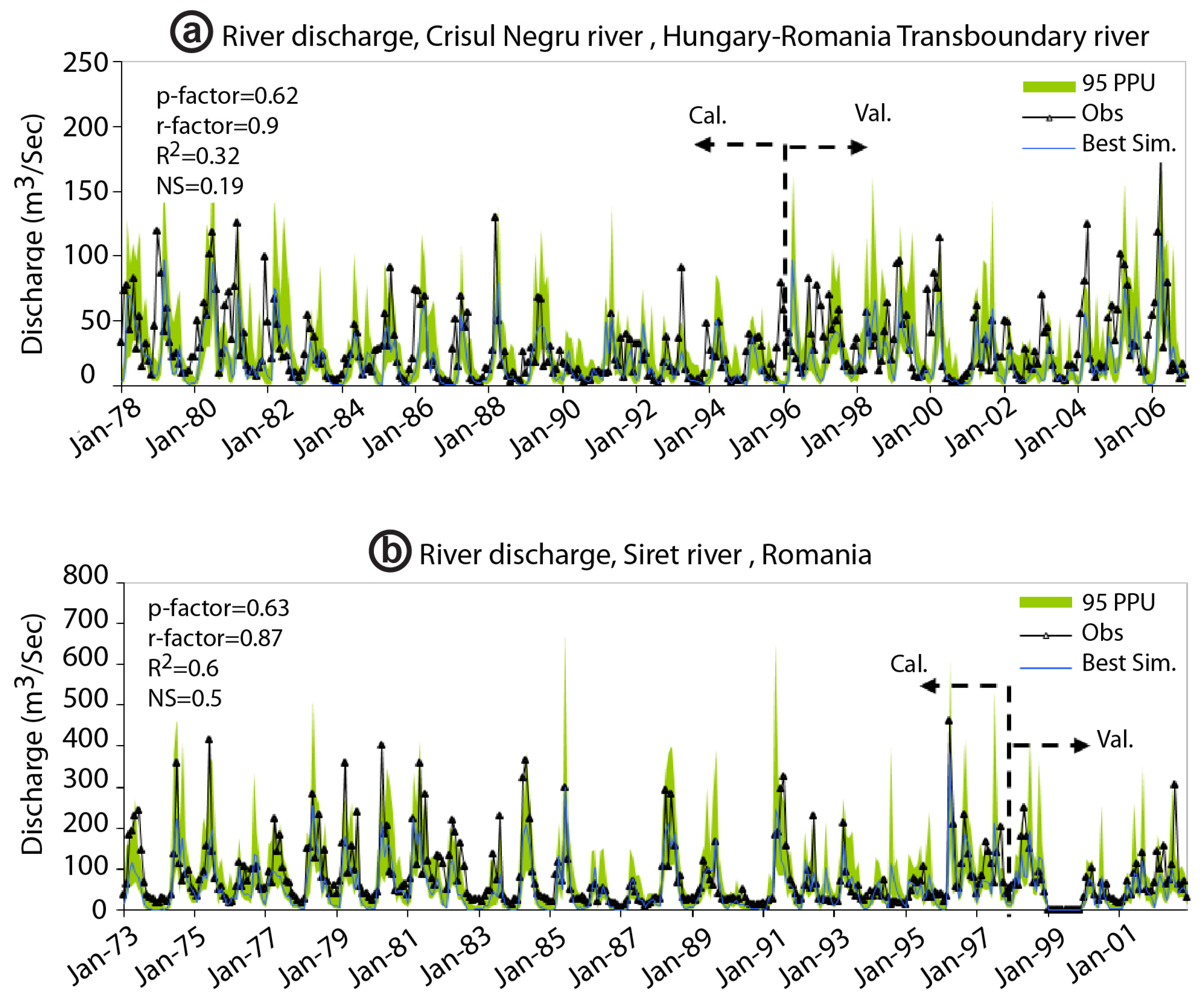
Figure 5.
Temperature distribution in the Black Sea Catchment: (a) average temperature, historic (1973–2006); (b) coefficient of variation (CV) of historic temperature (1973–2006); (c) average temperature HB scenario (2020–2050); (d) coefficient of variation of HB temperature (2020–2050); (e) average temperature HS scenario (2020–2050); (f) coefficient of variation of HS temperature (2020–2050); (g) deviation of HB future temperature scenario (2020–2050) from historic (1973–2006), °C; (h) deviation of HS future temperature scenario (2020–2050) from historic (1973–2006), °C.
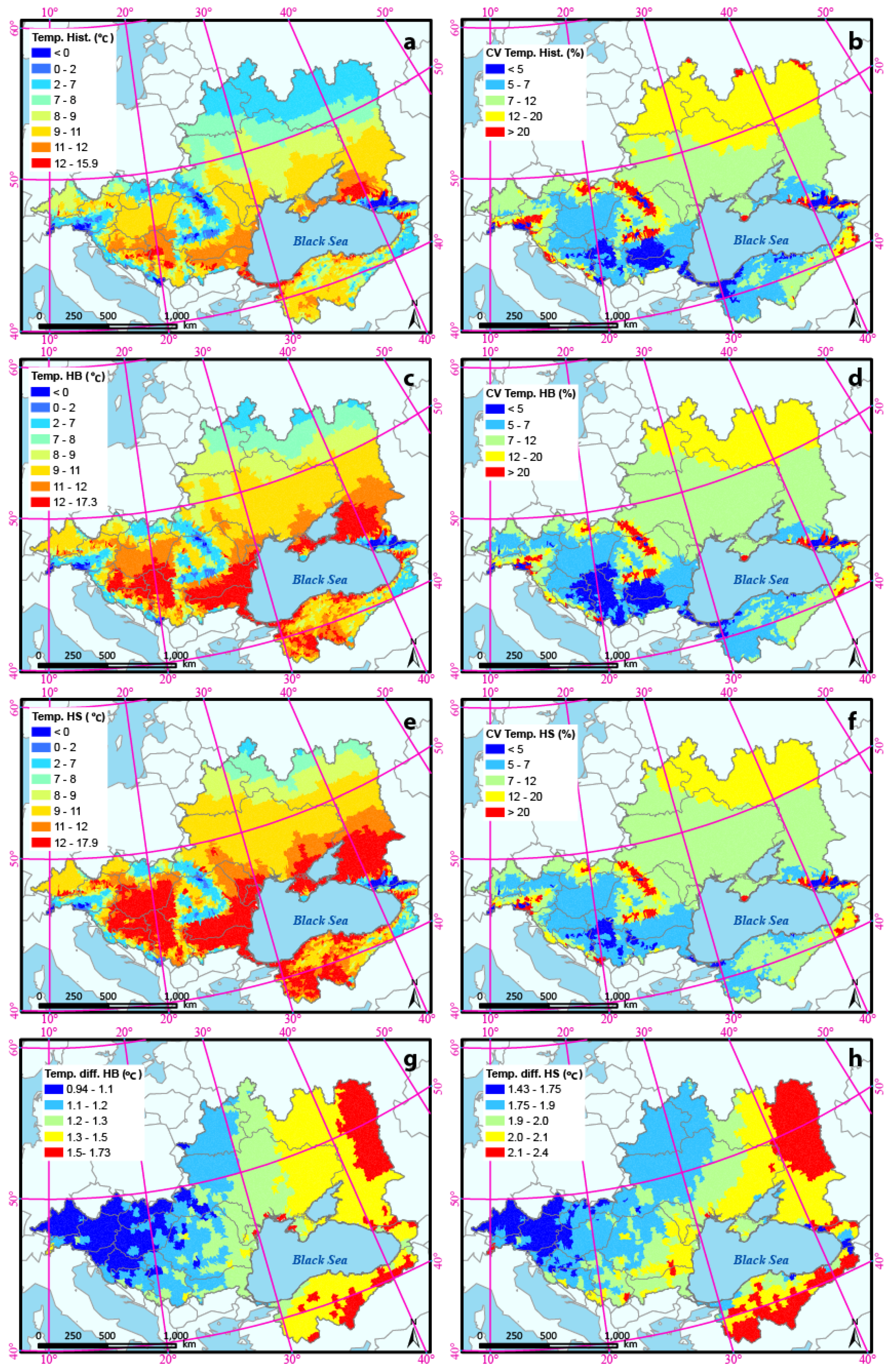
Figure 6.
Precipitation distribution in the Black Sea Catchment: (a) average precipitation, historic (1973–2006); (b) coefficient of variation of historic precipitation (1973–2006); (c) average precipitation HB scenario (2020–2050); (d) coefficient of variation of HB precipitation (2020–2050); (e) average precipitation HS scenario (2020–2050); (f) coefficient of variation of HS precipitation (2020–2050); (g) percent deviation of HB precipitation scenario (2020–2050) from historic (1973–2006); (h) percent deviation of HS precipitation scenario (2020–2050) from historic (1973–2006).

Figure 7.
Spatial distribution of blue water resources in the Black Sea Catchment: (a) long-term historical average (1973–2006); (b) temporal variation of historical blue water; (c) percent deviation of future blue water (2020–2050) from the historic (1973–2006) based on the ensemble of the 10 scenarios.

Figure 8.
Spatial distribution of green water storage (soil water) in the Black Sea Catchment: (a) long-term historical average (1973–2006); (b) coefficient of variation (temporal variation) of the green water storage (1973–2006); (c) percent deviation of future green water storage (2020–2050) from the historic (1973–2006); (d) coefficient of variation of average soil moisture among the 10 scenarios.
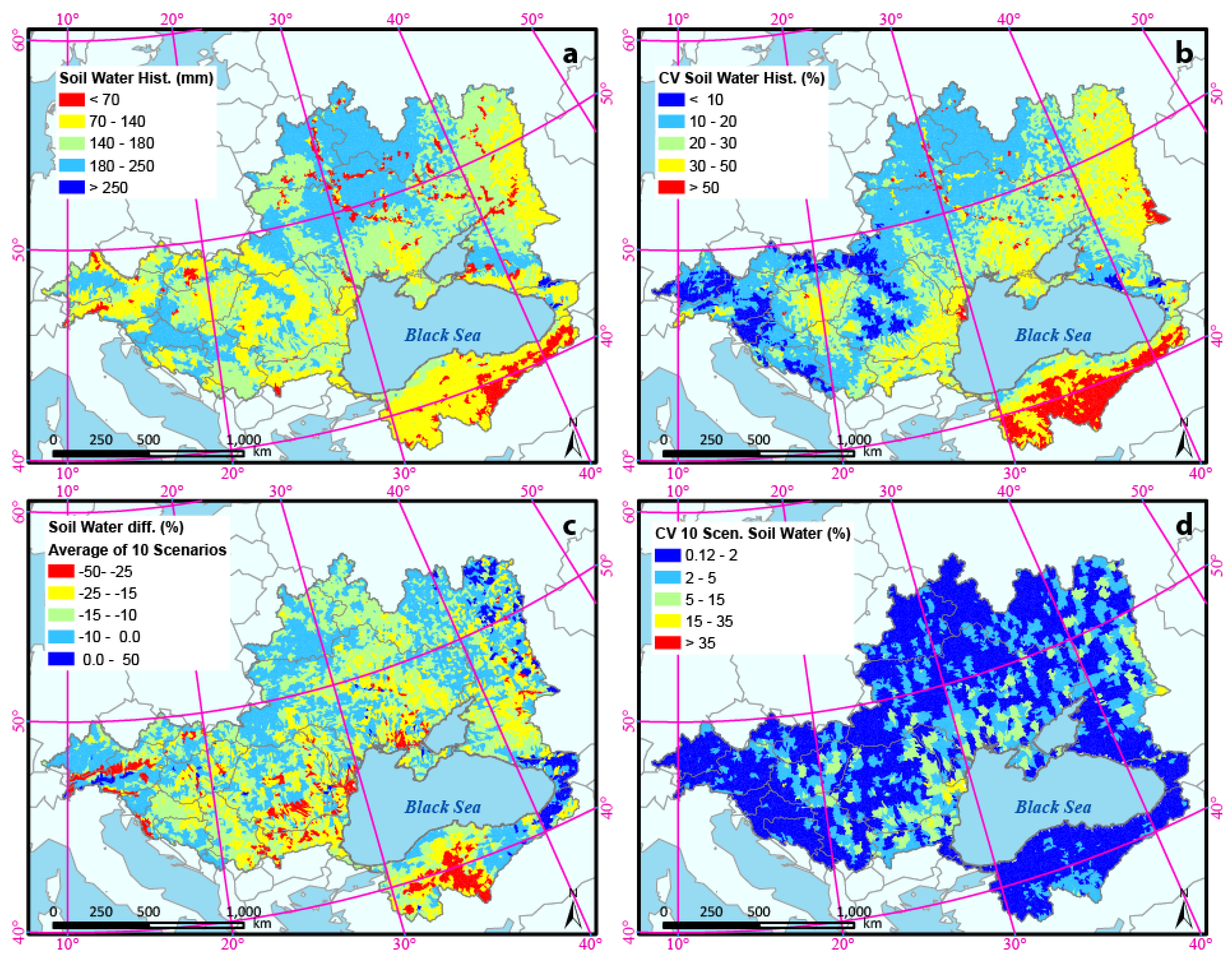
Figure 9.
Spatial distribution of green water flow (evapotranspiration) in the Black Sea Catchment: (a) long-term historical average (1973–2006); (b) temporal variation of the green water flow (1973–2006); (c) percent deviation of the future green water flow (2020–2050) from historic (1973–2006) based on the ensemble of 10 scenarios; (d) coefficient of variation of actual evapotranspiration among the 10 scenarios.
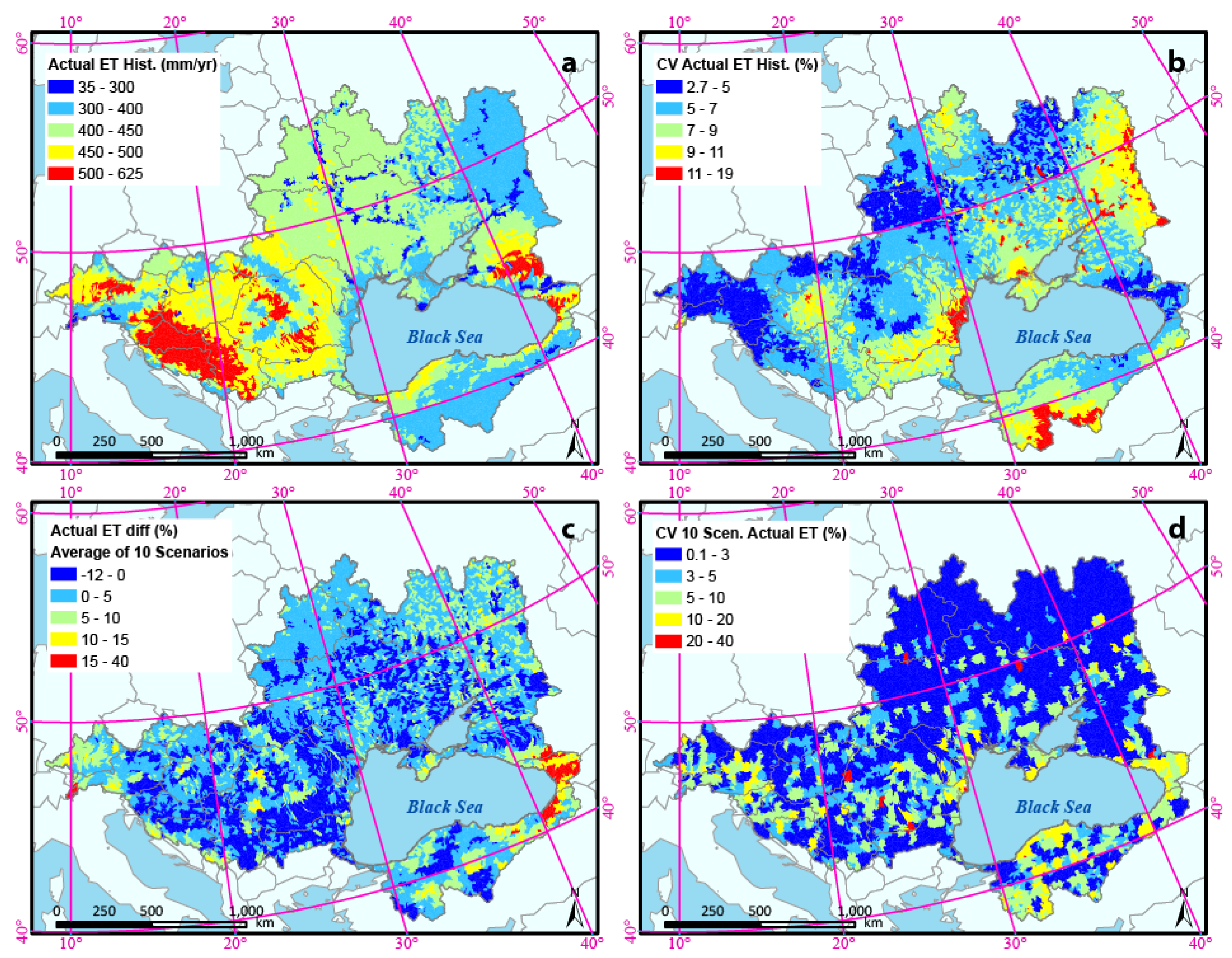
Figure 10.
Coefficient of variation (CV) of the model predictions using four future landuse scenarios (BS ALONE, BS COOL, BS COOP, and BS HOT) in combination with the HB future climate Scenario (left column) and the HS future climate scenario (right column). (a,b) blue water resources; (c,d) green water storage (soil moisture); (e,f) green water flow (evapotranspiration). LU, landuse.
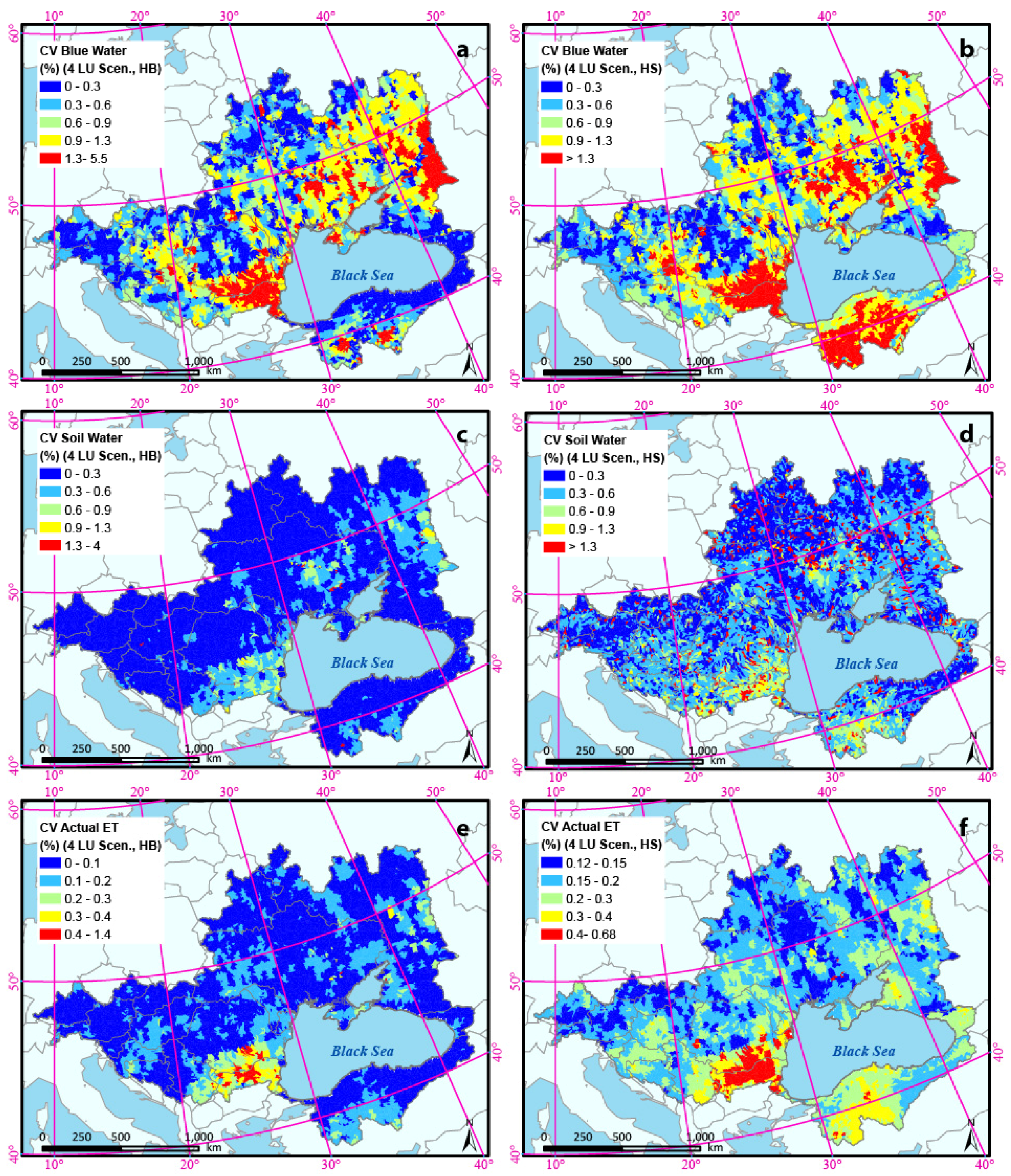
Figure 11.
Comparison of the number of wet days with >2 mm d−1 threshold (left column), and >10 mm d−1 threshold (right column) between the historic (1973–2006) and HB and HS future climate scenarios (2020–2050) for five selected sub-basins (a,b) a subbasin in Russia; (c,d) a subbasin in Ukraine; (e,f) a subbasin in Austria; (g,h) a subbasin in middle Danube; and (i,j) a subbasin in Turkey.


Table 1.
Summary of landuse trends and driving forces in the Black Sea Catchment’s scenarios.
| Landuse Scenarios | ||||
|---|---|---|---|---|
| Driving Forces | BS HOT | BS ALONE | BS COOP | BS COOL |
| Population growth | low | very high | low | medium |
| Urban population | increase | increase | slight increase | slight increase |
| GDP growth | very high | slow | high | medium |
| Forest area | increase | decrease | increase | decrease |
| Grassland area | increase | decrease | increase | decrease |
| Cropland area | increase | increase | decrease | increase |
| Built-up area | increase | increase | increase | stable |
| Protected areas | stable | stable | increase | stable |
| Climate change | high | high | lower | low |
Note: GDP, gross domestic product.
Table 2.
Sources of model input data and descriptions for the base model.
| Type | Source | Description |
|---|---|---|
| DEM | SRTM [33] | 90 m resolution extracted for BSC |
| Climate | CRU [30,34], Solar Radiation [35] | 0.5° resolution gridded climate data, daily temperature (min.; max.), daily precipitation (1970–2006) daily global solar radiation from 6110 virtual stations (1970–2006) |
| River | ECRINS [36] | 30 m resolution, from European Catchments and Rivers Network System (ECRINS) |
| Soil | FAO [37] | 5 km resolution, from FAO-UNESCO global soil map, provides data for 5000 soil types comprising two layers (0–30 cm and 30–100 cm depth) |
| Landuse | MODIS [22] | 500 m resolution, by the NASA Land Processes Distributed Active Archive Center (LP DAAC) at the USGS/Earth Resources Observation and Science Center (EROS) |
| Management | MIRCA2000 [38], McGill yields data [39] | 5 arc min resolution cropping area and the start and end month of cropping periods, 5 arc min crop yield of three major crop (Wheat, Cory, Barely) |
| River discharge | GRDC [40] | 144 Monthly river discharge data (1970–2006) |
Notes: DEM, Digital Elevation Model; SRTM, Shuttle Radar Topography Mission; BSC, Black Sea Catchment; CRU, Climate Research Unites; ECRINS, European Catchments and RIvers Network System; FAO, Food and Agriculture Organization; MODIS, Moderate Resolution Imaging Spectroradiometer; MIRCA, Monthly Irrigated and Rainfed Crop Areas; GRDC, Global Runoff Data Centre.
Table 3.
Soil and Water Assessment Tool (SWAT) processes used in the study.
| Processes/Components | Method |
|---|---|
| Evapotranspiration | Hargreaves |
| Surface runoff | Soil Conservation Service (SCS) curve number |
| Erosion | Modified universal soil loss equation |
| Lateral flow | Kinematic storage model |
| Groundwater flow | Steady-state response from shallow aquifer |
| Stream flow routing | Variable storage routing |
Table 4.
List of sensitive parameters used for model calibration.
| Parameter Name | Definition |
|---|---|
| CN2.mgt | SCS runoff curve number for moisture condition II |
| ALPHA_BF.gw | Base flow alpha factor (days) |
| GW_DELAY.gw | Groundwater delay time (days) |
| GWQMN.gw | Threshold depth of water in shallow aquifer for return flow (mm) |
| GW_REVAP.gw | Groundwater revap. coefficient |
| REVAPMN.gw | Threshold depth of water in the shallow aquifer for ‘revap’ (mm) |
| RCHRG_DP.gw | Deep aquifer percolation fraction |
| CH_N2.rte | Manning’s n value for main channel |
| CH_K2.rte | Effective hydraulic conductivity in the main channel (mm h−1) |
| ALPHA_BNK.rte | Baseflow alpha factor for bank storage (days) |
| SOL_AWC().sol | Soil available water storage capacity (mm H2O/mm soil) |
| SOL_K().sol | Soil conductivity (mm h−1) |
| SOL_BD().sol | Soil bulk density (g cm−3) |
| OV_N.hru | Manning’s n value for overland flow |
| HRU_SLP.hru | Average slope steepness (m m−1) |
| SLSUBBSN.hru | Average slope length (m) |
| SFTMP().sno | Snowfall temperature (°C) |
| SMTMP().sno | Snow melt base temperature (°C) |
| SMFMX().sno | Maximum melt rate for snow during the year (mm °C−1 day−1) |
| SMFMN().sno | Minimum melt rate for snow during the year (mm °C−1 day−1) |
Note: SCS, Soil Conservation Service.
© 2017 by the authors. Licensee MDPI, Basel, Switzerland. This article is an open access article distributed under the terms and conditions of the Creative Commons Attribution (CC BY) license (http://creativecommons.org/licenses/by/4.0/).
Share and Cite
MDPI and ACS Style
Rouholahnejad Freund, E.; Abbaspour, K.C.; Lehmann, A. Water Resources of the Black Sea Catchment under Future Climate and Landuse Change Projections. Water 2017, 9, 598. https://doi.org/10.3390/w9080598
AMA Style
Rouholahnejad Freund E, Abbaspour KC, Lehmann A. Water Resources of the Black Sea Catchment under Future Climate and Landuse Change Projections. Water. 2017; 9(8):598. https://doi.org/10.3390/w9080598
Chicago/Turabian StyleRouholahnejad Freund, Elham, Karim C. Abbaspour, and Anthony Lehmann. 2017. "Water Resources of the Black Sea Catchment under Future Climate and Landuse Change Projections" Water 9, no. 8: 598. https://doi.org/10.3390/w9080598
Note that from the first issue of 2016, this journal uses article numbers instead of page numbers. See further details here.