Distributed Hydrological Modeling: Determination of Theoretical Hydraulic Potential & Streamflow Simulation of Extreme Hydrometeorological Events

Abstract

The progressive change in climatic conditions worldwide has increased frequency and severity of extreme hydrometeorological events (EHEs). México is an example that has been affected by the occurrence of EHE leading to economic, social, and environmental losses. The objective of this research was to apply a Canadian distributed hydrological model (DHM) to tropical conditions and to evaluate its capacity to simulate flows in a basin in the central Gulf of Mexico. In addition, the DHM (once calibrated and validated) was used to calculate the theoretical hydraulic power (THP) and the performance to predict streamflow before the presence of an EHE. The results of the DHM show that the goodness of fit indicators between the observed and simulated flows in the calibration process Nash-Sutcliffe efficiency (NSE) = 0.83, ratio of the root mean square error to the standard deviation of measured data (RSR) = 0.41, and percent bias (PBIAS) = −4.3) and validation (NSE = 0.775, RSR = 0.4735, and PBIAS = 2.45) are satisfactory. The DHM showed its applicability: determination of THP showed that the mean flows are in synchrony with the order of the river reaches and streamflow simulation of 13 EHEs (NSE = 0.78 ± 0.13, RSR = 0.46 ± 0.14 and PBIAS = −0.48 ± 7.5) confirmed a reliable efficiency. This work can serve as a tool for identifying vulnerabilities before floods and for the rational and sustainable management of water resources.

1. Introduction

The progressive change in climatic conditions worldwide has caused an increase in the frequency and severity of extreme hydrometeorological events (EHEs) [1]. Mexico, because of its geographic location and physical characteristics, is vulnerable to the occurrence of EHEs—mainly to the formation and development of tropical cyclones on the Pacific coast and the Gulf of Mexico that affect 60% of the national territory.

According to the last Official Statistics of the National Center for Disaster Prevention (Centro Nacional de Prevención de Desastres, CENAPRED), more than 2500 people have died because of EHE disasters (droughts, rains, cyclones), including 535 who died in tropical storms and hurricanes [2].

Located in the central part of the Gulf of Mexico, Veracruz State, due to its geographical location, orography, climate and human settlements in high risk areas, is a highly vulnerable area vulnerable exposed to these phenomena. This province was affected by three huge EHEs: a tropical storm (2000) and two hurricanes (Stan 2005 and Karl 2010) causing substantial economic, social, and environmental losses. In addition, the surface water potential of the state of Veracruz is among the highest in Mexico [3], with an average annual surface runoff estimated at 121 million cubic meters, representing 33% of the surface runoff of the entire country [4]. According to Larios-Tlali et al., 2015 [5] Veracruz has an area of 72,815 km², and 73% of its territory is below 200 msnm [6]. The local authorities (State Government of Veracruz) [7] report a floodable area of 6275 km² (8% of the state territory) in 2189 localities within 118 municipalities. As a result, one in every six citizen in the State of Veracruz is affected by floods.

Despite the importance of EHEs in recent decades, there are many limitations regarding the availability and quality of hydrometeorological data [8]. Predicting the temporal behavior of the rainfall-streamflow phenomena is a task that requires formal research [9]. Considering the deficiencies in the data and the urgency to prevent further socio-economic losses due to floods, it is necessary to develop scientifically based tools for an accurate prediction of their consequences [10]. One solution is the use of hydrological simulation models due to their low operating cost [11]. Therefore, the main objective of this research were (1) to evaluate the rainfall-runoff response of the distributed hydrological model (HYDROTEL) under tropical conditions and (2) to evaluate the response of the distributed hydrological model (HYDROTEL) in two applications: the forecast of runoff from EHEs and the determination of theoretical hydraulic power along a basin.

2. Case Study: La Antigua River Basin in Veracruz, México

The watershed is located in the central part of the Gulf of Mexico between 19°12′′ and 19°35′′ north latitudes and between 96°30′′ and 97°13′′ west longitudes (Figure 1), which is exposed to a great variety of EHEs, such as hurricanes, tropical storms, and floods. These EHEs become disasters when they cause harm to human populations and affect their economy and infrastructure [12].

The zone of study has an approximate area of 1620.6 km² with an elevation ranging from 4204 m a.s.l. to 82 m a.s.l. Due to its high altitudinal variation, there are great climatic variations and differing vegetation covers throughout the basin. The precipitation in the watershed varies between 1500 mm and 2500 mm, whilst the average annual temperature is between 18 °C to 26 °C [4]. The main soils present in the study area are acrisol (68.6%) located in the north of basin, luvisol (23.8%) in the centre, podzol (3.6%), and vertisol (4%) in the south [14]. The types of land uses include agriculture (57.3%), urban area (2.1%), forest (17.8%), and pastureland (22.8%) [15]. Agriculture in this basin is a mix between rainfed and irrigated agriculture (having as main crops sugar cane, coffee, corn, mango, and lemon, among others), and the basin supplies water to the cities of Xalapa and Coatepec [15].

3. Materials and Methods

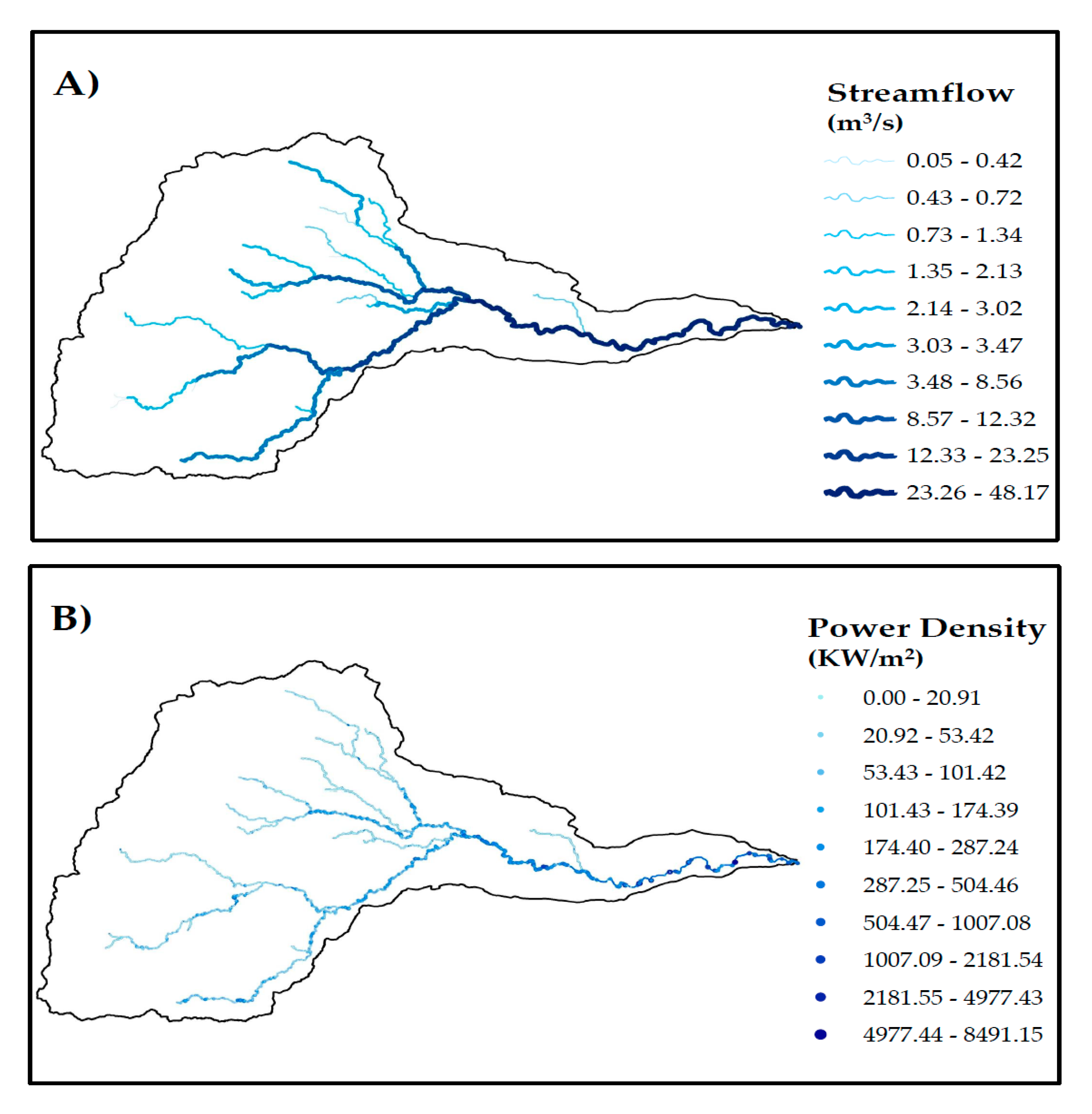
This research was divided in five stages: (1) data collection and analysis; (2) application of HYDROTEL model to the basin under study; (3) calibration of the hydrological model; (4) spatial and temporal validation of the hydrological model; and (5) applications of distributed hydrological model: theoretical hydraulic potential estimation and streamflow simulation of extreme hydrometeorological events.

3.1. Data Collection and Analysis

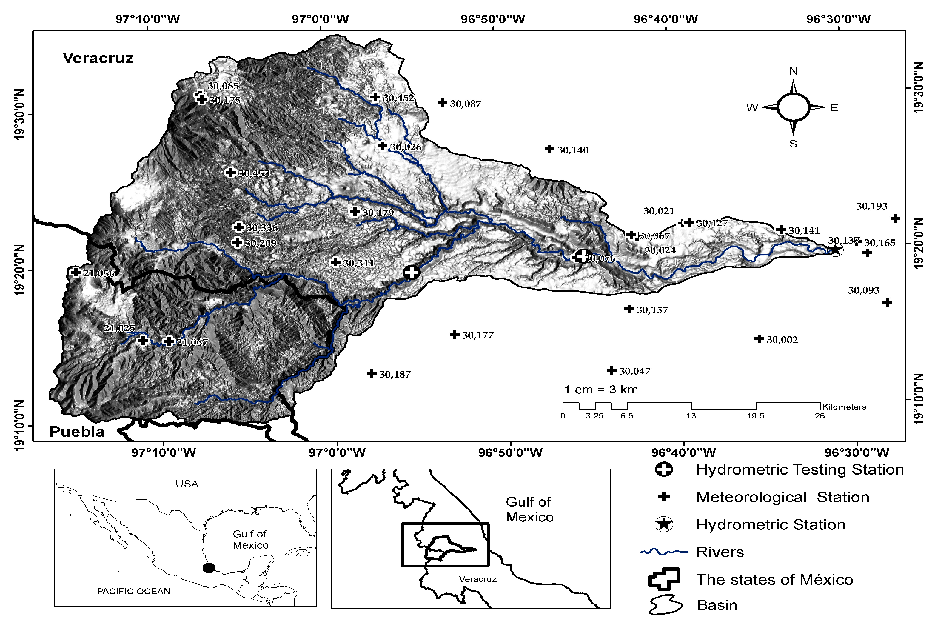
The essential data for distributed hydrological modeling requires two types of information: hydrometeorological and physiographic databases. The first class of data is required on a daily basis for the following variables: minimum temperature, maximum temperature, total precipitation, and streamflow at the outlet of the basin. The second class of data includes the digital elevation model, the land uses, and types of soil.

Subsequently, the data was subjected to a quality control, with the objective of detecting errors in the observation data that could be caused mainly by difficulties in the measurement plus errors due to manipulation and data capture and storage processes. These processes apply to the identification of errors, such as the maximum temperature being greater than the minimum or the precipitation being negative. Other errors have been filtered because they are outside the range of values of the region, such as temperatures above 50 °C or lower than −25 °C [16].

Description of the Geographic Information System “PHYSITEL”

PHYSITEL [17] was developed at the INRS-ETE (Institut national de la recherche scientifique centre Eau, Terre et Environnement) in Québec, Canada in 1985 [18]. It is designed to be used in the preparation of the physiographic database of the HYDROTEL hydrological model [19]. It allows the integration of various types of data from remote sensing and geographical information systems (GIS). The data used by PHYSITEL are of the raster type (DEM, soil types, and land use) and vector type (hydrographic network, limit of the watershed). PHYSITEL allows characterizing the internal flow structure of a watershed from a numerical elevation model. The determination of the internal flow structure serves as a basis for the characterization of the hydrological units (or sub-basins) that represent the spatial simulation units [20].

The information on the surface conditions that affect the “evaporation-flow-infiltration” can be integrated to determine the hydrological parameters of the calculation units. PHYSITEL defines the watershed into relatively homogeneous hydrological units (RHHUs) [21]. These hydrological units are established to contain only one section of the hydrological network. To each of these units is assigned a single value for soil type, which corresponds to the dominant formation for the entire unit. 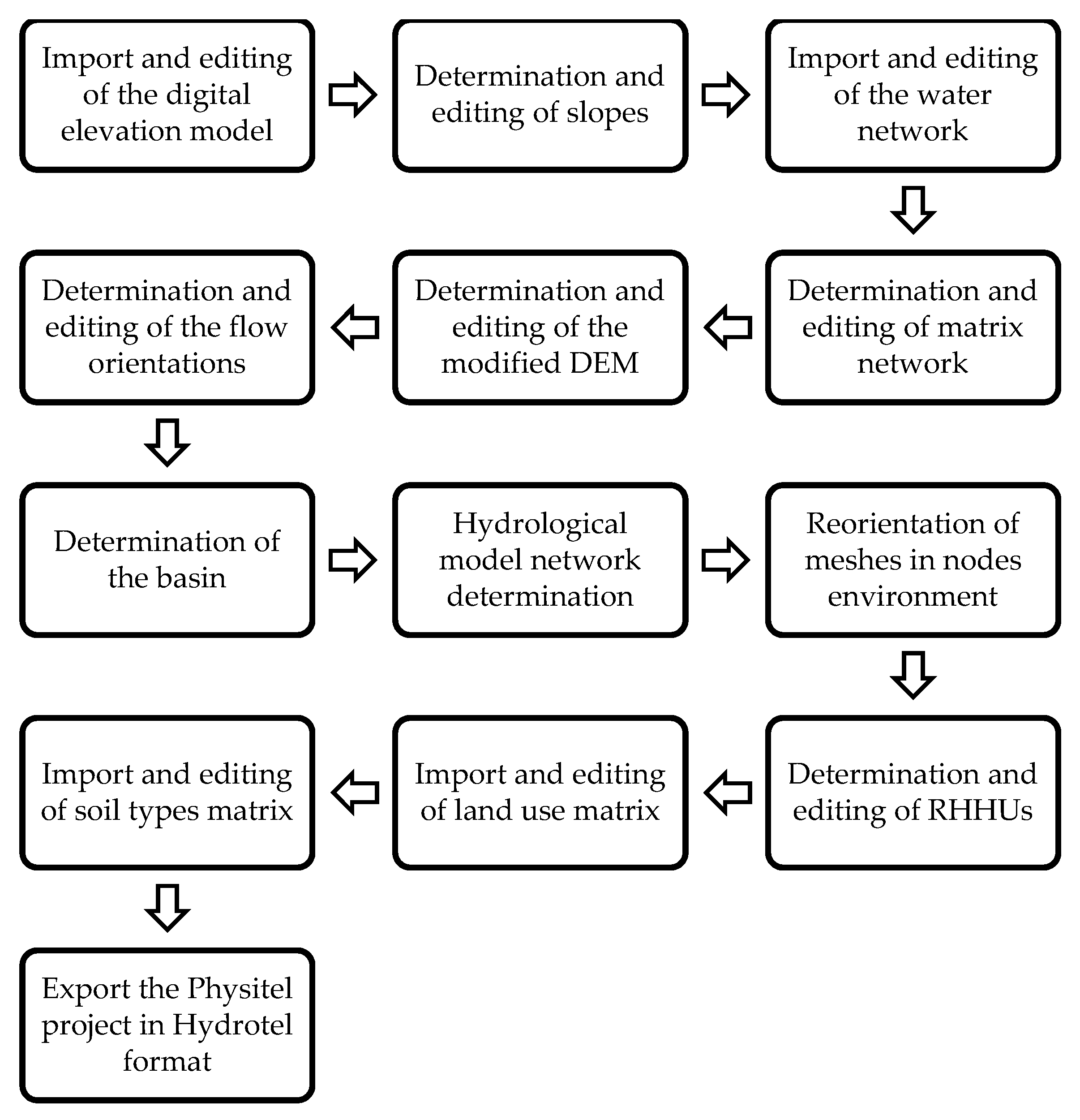Each one of these units is also assigned the percentages represented by each land-use class [17,21]. At the end, PHYSITEL allows us to export to HYDROTEL the following data: altitude, slope, flow orientation, hydrographic network, and delineation of each RHHU, based on a user defined threshold that is set according to the desired level of detail. Figure 2 shows a block diagram of each characterization and quantification stage when PHYSITEL was utilized.

3.2. Application of the Distributed Hydrological Model (HYDROTEL)

HYDROTEL [22] was developed by the INRS-ETE. It is a spatially distributed hydrological model with physical bases specifically developed to facilitate the use of remote sensing and GIS data. This approach brings a better representation of the spatial variability of the physiographic characteristics of river basins (topography, land use, soil types, etc.) and of the meteorological systems that affect the basins [23].

HYDROTEL comprises six submodules, which run in successive steps. Each Submodule simulates a specific hydrological process.

The first submodule is the Interpolation of meteorological data: this module deals with the interpolation of meteorological variables, including liquid or solid precipitation, minimum and maximum temperatures, relative humidity, wind speed, and solar radiation (when the later three are available; the model can run based on temperature and precipitation data only, and the required input data depends on the selected modeling options as described hereafter). There are two simulation options: thiessen’s polygons or weighted mean of nearest three stations.

The second submodule is the Snow cover estimation: this module simulates the accumulation and melt of snowpack in each RHHU. It simulates daily changes of mean snowpack characteristics (thickness, water equivalent, mean density, thermal deficit, liquid water content, and temperature) using a modified energy budget approach developed by Riley et al., 1973 [24] (for a complete description, see Turcotte et al., 2007 [25]).

The third submodule is the Potential evapotranspiration (PET) estimation: this module calculates the PET for each RHHU using a choice of equations depending on available meteorological data: (i) Thornthwaite (1948) [26]; (ii) Linacre (1977) [27]; (iii) Penman–Monteith [28]; (iv) Priestley and Taylor (1972) [29], or (v) formulation developed by Hydro-Québec.

The fourth submodule is the Vertical water balance: the soil column moisture, rainfall, and/or snow melt are partitioned into infiltration and runoff. For simulation purposes, the soil column is divided into three layers. The first layer controls infiltration, the second layer can be associated with interflow, and the third layer with base flow. There are also two simulation options: vertical balance of three layers (BV3C) and the vertical water budget based on the CEQUEAU hydrological model [17,18,19].

The fifth submodule is the Overland routing: this is the surface and subsurface flow transfer module. The available amount of free water from each soil layer of an RHHU is summed up and routed to the corresponding downslope to the river segments using an RHHU-specific geomorphological unit hydrograph (GUH) [17,18,19]. This hydrograph is determined once for each RHHU using the kinematic wave approximation of the complete Saint-Venant system of equations, but is can be recomputed if necessary. For example, when there is a change in land cover. The shape of the specific GUH is determined by routing a reference water depth over all cells of na RHHU based on the slope and roughness of each cell. The resulting values are considered as lateral inflow to the river segment draining the RHHU [23].

The sixth submodule is the Channel routing: two simulation options are the diffusive and the kinematic wave equations, both being approximations of the Saint-Venant equations. For more details on these aspects of HYDROTEL, the reader is referred to Fortin et al., 2001 [19].

3.3. Calibration of the Distributed Hydrological Model

The hydrological models constitute an important tool in the management of surface water and therefore in hydro-informatics. In order to successfully implement these models, they have to be calibrated. In the calibration process of the model, the values of the parameters are identified, with the aim of improving the goodness of fit between the simulated data time series and the observed data. To evaluate the goodness of fit of the model, an “objective function” is used. This process can be performed in two ways: test-error (manually) and automatically. In the latter case, the calibration is performed using an optimization algorithm that is linked to the hydrological model [30].

In this study, the Dynamically Dimensioned Search (DDS) algorithm was used. It is designed to be an efficient tool for calibration of complex and large-parameter-space hydrological models [31]. The DDS algorithm automatically scales the search space to decrease the number of model evaluations required to reach the optimal region of best-quality fitness function [32]. The single DDS parameter was set to the default value, as recommended by the authors of the algorithm (for more details about the DDS algorithm, refer to Tolson and Shoemaker [32].

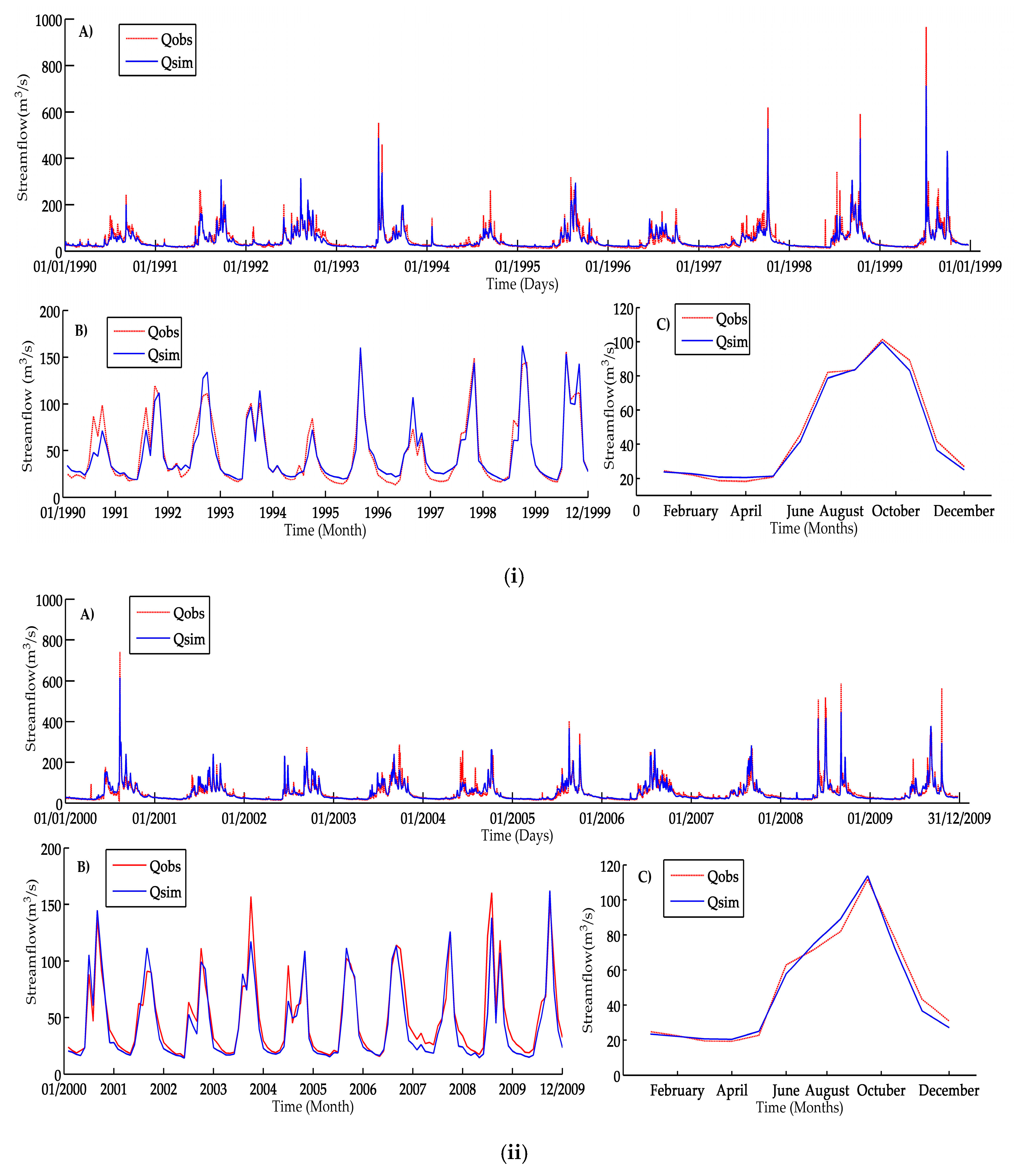
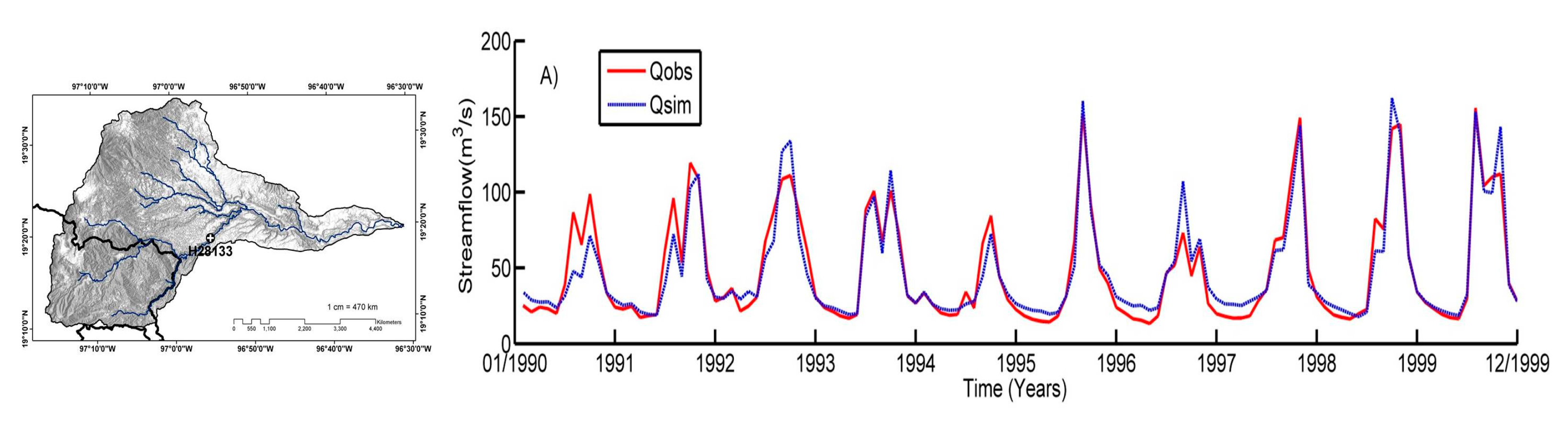
The calibration was evaluated by the statistical indicators. The indicators used in this study are the ones recommended by Moriasi et al., 2007 [33], namely the Nash-Sutcliffe model efficiency index, which is equal to one minus the ratio of the Mean Square Error (MSE) and standard deviation of measured data time series [34]. The Nash-Sutcliffe efficiency (NSE) [35] is computed as the relative magnitude of the residual variance compared to the variance of the observed data “information”. The NSE is shown in Equation (1) (see also

Table 1. Interpretation of statistical parameters for calibration and validation [33].

PBIAS	NSE	RSR	Interpretation of the Model
PBIAS < ±10	0.75 < NSE < 1.0	0.00 < RSR < 0.50	Very good
±10 < PBIAS < ±15	0.65 < NSE < 0.75	0.50 < RSR < 0.60	Good
±15 < PBIAS < ±25	0.50 < NSE < 0.65	0.60 < RSR < 0.70	Satisfactory
PBIAS > ±25	NSE < 0.50	RSR > 0.70	Unsatisfactory

Notes: PBIAS, percent bias; NSE, Nash-Sutcliffe efficiency; RSR, RMSE-observations standard deviation ratio.

for signification of the NSE values).

$$NSE=1-\left[\frac{{{\displaystyle \sum _{i=1}^n\left(q\left(i\right)-\stackrel{⌢}{q}\left(i\right)\right)}}^2}{{\displaystyle \sum _{i=1}^n{\left(q\left(i\right)-\overline{q}\right)}^2}}\right]$$

(1)

where $\widehat{q}\left(i\right)$ is the ith observation for the constituent being evaluated, $q\left(i\right)$ is the ith simulated value for the constituent being evaluated, $\overline{q}$ is the mean of observed data for the constituent being evaluated, and n is the total number of observations. NSE ranges between −∞ and 1.0 (1 inclusive), with NSE = 1 meaning a perfect match between simulated and observed values. Values between 0.0 and 1.0 are generally viewed as acceptable levels of performance (Table 1), whereas negative values mean that the mean of observed data is a better predictor than the simulated data [35].

The RMSE-observations standard deviation ratio (RSR) is calculated as the ratio of the Root Mean Square Error (RMSE) and standard deviation of measured data (Equation (2)) and was developed based on the recommendation by Singh et al. [36] RSR combines both an error index and the additional information recommended by Legates and McCabe [37]. An RSR of zero indicates the optimal value, while RSR > 0.7 represents unsatisfactory model performance [38] as shown in Table 1.

$$RSR=\frac{RMSE}{STDE{V}_{OBS}}=\frac{\left[\sqrt{{\displaystyle \sum _{i=1}^n{\left(q\left(i\right)-\stackrel{⌢}{q}\left(i\right)\right)}^2}}\right]}{\left[\sqrt{{\displaystyle \sum _{i=1}^n{\left(q\left(i\right)-\overline{q}\right)}^2}}\right]}$$

(2)

Percent bias (PBIAS) is the relative bias of data being evaluated, expressed as a percentage. PBIAS measures the average tendency of the simulated data to be larger or smaller than their observed counterparts [39]. The optimal value of PBIAS is 0.0, with low-magnitude values indicating accurate model simulation. Positive values indicate model underestimation PBIAS and negative values indicate model overestimation PBIAS [36,37] (see Table 1). PBIAS is calculated with Equation (3):

$$PBIAS=\left[\frac{{\displaystyle \sum _{i=1}^n\left(q\left(i\right)-\stackrel{⌢}{q}\left(i\right)\right)\times 100}}{{\displaystyle \sum _{i=1}^{n}q\left(i\right)}}\right]$$

(3)

3.4. Spatial and Temporal Validation of the Distributed Hydrological Model

The process of temporal validation of a model consists in demonstrating that the model is able to make predictions at a specific site for periods outside the calibration period. In this way, it is said that a model has been validated if its accuracy and predictive ability in the validation period showed acceptable errors or limits [40] . The calibration and validation was based on the hydrometric data of a control station located at the outlet of the studied river basin. The spatial validation process was carried out by applying the model to predict streamflow at other points within the basin. The validation was done with the same parameters obtained from calibration based on the hydrometric output station.

3.5. Applications of Distributed Hydrological Model: Theoretical Hydraulic Potential Estimation and Streamflow Simulation of Extreme Hydrometeorological Events

3.5.1. Estimation of Theoretical Hydraulic Potential

For the determination of the hydraulic potential, the following variables were calculated: (i) gross height (H_b) which was determined by means of DEM and ArcMap and (ii) P, the theoretical hydraulic power (KW), which was calculated using Equation (4) [41].

$$\mathrm{P}=\mathsf{\rho }\mathrm{g}\mathrm{Q}{\mathrm{H}}_{\mathrm{b}}$$

(4)

where Q is the mean annual flow rate in (m³/s), ρ is the water density and for the calculation is taken as 1000 kg/m³, g represents the acceleration of gravity (9.8 m/s²), and H_b is the gross height expressed in meters. It was estimated along the river reaches of the study basin [41].

3.5.2. Simulation of Extreme Hydrometeorological Events

Once the distributed hydrological model (HYDROTEL) was calibrated and validated, the EHEs that affected the study area from 1990 to 2009 in the study area (compiled from the NMS and underground weather reports), were simulated and subsequently evaluated by performance indicators (NSE, RSR, and PBIAS).

4. Results

4.1. Review and Analysis of the Available Hydrometeorological Data

In a first step, meteorological stations were selected (see

Table 2. Main characteristics of the meteorological stations of the study basin: key meteorological station, geographic coordinates, altitude (m a.s.l.), information time window, and state [42].

Key	Latitude	Longitude	Altitude	Start	End	State
21,025 A	19.26	−97.18	2220	1 March 1964	31 May 1997	Suspended
21,056 A	19.33	−97.25	1720	1 March 1964	31 July 2000	Operating
21,067 A	19.25	−97.16	2070	1 March 1964	31 December 2008	Operating
30,002 B	19.21	−96.59	410	1 March 1964	31 May 1997	Suspended
30,021 B	19.36	−96.66	420	1 June 1967	31 December 2008	Operating
30,024 B	19.35	−96.71	480	1 March 1964	31 December 1982	Suspended
30,026 B	19.46	−96.94	1252	1 January 1961	31 December 2008	Operating
30,047 B	19.17	−96.7	610	1 March 1964	31 January 2009	Operating
30,076 B	19.33	−96.76	335	1 January 1961	30 September 2009	Operating
30,085 B	19.52	−97.12	2959	1 October 1964	31 May 1997	Suspended
30,087 B	19.5	−96.89	1150	1 June 1953	30 June 1993	Suspended
30,093 B	19.26	−96.39	50	1 May 1951	31 December 2008	Operating
30,127 B	19.36	−96.66	425	1 January 2000	31 December 2010	Operating
30,137 B	19.33	−96.48	110	1 March 1964	31 August 2009	Operating
30,140 B	19.45	−96.78	880	1 January 1969	31 December 2008	Operating
30,141 B	19.35	−96.56	313	1 January 1921	31 December 2008	Operating
30,157 B	19.27	−96.71	350	1 March 1964	31 May 1997	Suspended
30,165 B	19.34	−96.49	144	1 May 1956	31 December 2008	Operating
30,175 B	19.51	−97.12	3110	1 October 1965	31 December 2008	Operating
30,177 B	19.25	−96.88	1100	1 March 1964	31 May 2005	Operating
30,179 B	19.39	−96.97	1218	1 August 1944	31 December 2008	Operating
30,187 B	19.21	−96.96	1446	1 May 1959	31 December 2008	Operating
30,193 B	19.36	−96.37	28	1 January 1941	31 December 2008	Operating
30,209 B	19.36	−97.12	1785	1 March 1964	30 September 2009	Operating
30,311 B	19.33	−96.99	1225	1 April 1976	31 December 2008	Operating
30,336 B	19.36	−97.12	1785	1 January 1980	31 December 2007	Operating
30,367 B	19.35	−96.71	523	1 January 1981	31 January 1996	Suspended
30,452 B	19.51	−96.95	1320	1 July 1984	31 December 2008	Operating
30,453 B	19.43	−97.09	2080	1 January 1995	31 December 2008	Operating

Note: Stations located in Puebla (^A) and for Veracruz (^B).

) on two conditions. The first selection criterion was temporality, ensuring that the selected stations have information over the time period, for which streamflows are available i.e., from 1 January 1990 to 31 December 2009. The second criterion ensured that selected stations were located within the buffer of 5 km from the study watershed. Meteorological data were obtained from the National Weather Service (Servicio Meteorológico Nacional-SMN-) [42] and hydrometric data (stations H28125-outlet, and H28133 and H28134—within the river basin) were obtained from the National data bank on Surface Water (Banco Nacional de Aguas Superficiales -BANDAS-) [43] for the same period.

4.2. Selecting Algorithms for the Simulation of Hydrological Processes

The study area covers 1621 km². It was discretized in 33 hydrological units or RHHUs with an average area of 50 m². Then, percentages of each soil type and predominant soil texture were added to each RHHU. The following simulation options were selected for each one of the HYDROTEL submodules (see Section 3.2): (i) interpolation of meteorological data: weighted mean of nearest three stations; (ii) snow cover estimation: mixed approach (deg.day—energy balance, which is the only available option); (iii) potential evapotranspiration: Hydro-Québec; (iv) vertical water balance: three layer vertical water balance (BV3C), (v) Overland routing: kinematic wave (which is the only available option), and (vi) channel routing: kinematic wave [18].

4.3. Calibration and Validation of the Distributed Hydrological Model (HYDROTEL)

The parameters of hydrological model (see

Table 3. Parameters of the distributed hydrological model.

Key	Parameters to Be Optimized	Units
Z1	Depth of the lower boundary of soil layer # 1 (2)	m
Z2	Depth of the lower boundary of soil layer # 2 (2)	m
Z3	Depth of the lower boundary of soil layer # 3 (2)	m
EF	Environments forests	ADIM
EC	Extinction coefficient (2)	ADIM
DSMAX	Maximum variation of humidity (2)	kg/m3
MFCF	Melt factor for coniferous forests (1)	mm/d °C
MFDF	Melt factor for deciduous forests (1)	mm/d °C
MFOA	Melt factor for open areas (1)	mm/d °C
MRSS	Melt rate at the snow–soil interface (1)	mm/d
PET	Potential evapotranspiration multiplication factor (1)	ADIM
RC	Recession coefficient (2)	m/h
GH	Reference runoff depth for the geomorphologic hydrograph	M
TMC	Threshold air temperature for melt in coniferous forests (1)	°C
TMD	Threshold air temperature for melt in deciduous forests (1)	°C
TMOA	Threshold air temperature for melt in open areas (1)	°C
TTSL	Threshold air temperature for partitioning solid and liquid precipitation (1)	°C
VGP	Vertical gradient of precipitation	mm/100 m
VGT	Vertical gradient of temperature	°C/100 m

Notes: (¹) For a complete description of snow parameters, the reader is referred to Turcotte et al., 2007 [25]. (²) For a complete description of soil parameters, the reader is referred to Fortin et al., 2001 [19].

) were automatically calibrated using the Dynamically Dimensioned Search (DDS) algorithm in order to achieve an acceptable level of statistical performance according to Moriasi et al., 2007. The three statistical indicators introduced in Section 3.3 were used: NSE, RSR, and PBIAS. The calibration was performed on the basis of observed flow data.

The DDS method looks for an optimal set of parameters within a limited parameter space based on the Nash-Sutcliffe efficiency criterion maximization. An initial set of parameters can be specified by the user or not (in this case, random initials parameters were used, in a logical range for each of them), and the total number of model evaluations allowed for the calibration process was set to 10,000 [31].

Split Sample [44] was used for calibration and validation process. The data time series that was used for calibration spans from 1 January 1990 to 31 December 1999 (10 years). The following criteria lead to the choice of this 10-years period: (1) the length remained reasonable due to computational time considerations with HYDROTEL, (2) the years had to be consecutive to facilitate the execution of the simulation with HYDROTEL, both for the calibration and validation periods, and (3) the availability of hydrometeorological information [45].

4.3.1. Temporal Validation of Hydrologic Modeling

Temporal validation of the model was performed over a 10-year period that spans from 1 January 2000 to 31 December 2009. Daily and monthly hydrographs for the entire calibration and validation periods, as well as mean annual hydrographs based on monthly mean values are show in Figure 3. Overall, the model reproduces very well the mean annual hydrograph and also yields very good results for daily and monthly streamflows in both the calibration and validation periods. In the calibration period, low flows are often overestimated by the model (about 8.4% on average; Figure 3(iB)). In both periods, some peaks are underestimated by the model (Figure 3(iA,iB,iiA,iiB); about 6.15% on average).

Table 4. Results of the statistical indicators that evaluate the performance of the calibration and validation of the distributed hydrological model, calculated from daily and mean monthly time series, in La Antigua River basin.

Process	Statistic	Daily	Description	Monthly	Description
Calibration	NSE	0.8321	Very Good	0.929	Very Good
	RSR	0.41	Very Good	0.2685	Very Good
	PBIAS	−4.3	Very Good	−4.2834	Very Good
Validation	NSE	0.775	Very Good	0.909	Very Good
	RSR	0.4735	Very Good	0.3014	Very Good
	PBIAS	2.45	Very Good	2.188	Very Good

, presents the statistical indicators (NSE, PBIAS, and RSR) that were calculated using the daily and monthly observed and simulated streamflows for the calibration (1990–1999) and validation (2000–2009) periods in the La Antigua basin. The statistical indicators are systematically higher in the monthly scale. This is probably explained by the fact that monthly values are averages of already very good daily simulated values. In the monthly averages, the variations that affect the indicators on a smaller temporal time step are smoothed. It was also detected that PBIAS values showed that the model underestimated the values during the calibration and validation periods. In conclusion, the results are satisfactory according to Moriasi et al., 2007 [33].

4.3.2. Spatial Validation of the Distributed Hydrologic Modeling

The spatial validation was performed for two additional hydrometric stations (H28133 and H28134) located within the study area for the same time period. The results are shown in

Table 5. Statistical parameters of performance in series from daily and monthly data for the two test points (H28133 and H28134) the evaluation period from 1 January 1990 to 31 December1999.

Test Points	Statistic	Daily	Description	Monthly	Description
H28133	NSE	0.62	Good	0.78	Very Good
	RSR	0.59	Good	0.39	Very Good
	PBIAS	−5.83	Very Good	−5.40	Very Good
H28134	NSE	0.70	Good	0.82499	Very Good
	RSR	0.54	Good	0.45	Very Good
	PBIAS	−6.86	Very Good	−6.27	Very Good

and in Figure 4. It is noteworthy that these hydrometric stations were not taken into account for the calibration process.

Table 5 shows that, in general, the model performs well or very well, with NSE values of 0.62 and 0.70 for daily streamflows, and NSE of 0.78 and 0.82 for monthly streamflows. Figure 4 shows the quality of the model when simultaneously drawing the monthly observed and simulated hydrographs at the two points used for spatial validation.

4.4. Application of Distributed Hydrological Modeling: Determination of Theoretical Hydraulic Potential and Streamflow Simulation of Hydrometeorological Extreme Events

4.4.1. Estimation of Theoretical Hydraulic Potential

Once the distributed hydrological model presents a satisfactory adjustment and its performance can be classified as acceptable (or better), an application of the model is a calculation of the hydraulic potential of a hydrographic basin; this was possible with the use of the distributed hydrological modeling and tools of a GIS. The results of runoff distribution are shown in Figure 5.

Figure 5A shows that the mean flows are in synchrony with the order of the river reaches (more flow to higher order river reaches). It is also observed that the northern branch of the basin contributes more to the streamflow at the outlet because of a greater number of river reaches and their higher orders. Flows values ranges from 0.05 m³/s to 48.17 m³/s. In Figure 5B, the highest values of power density are in the central zone and generally follow the mean flow values (Figure 5A). The power density varies from 0.001 KW/m² to 8491.15 KW/m².

4.4.2. Streamflow Simulation of Extreme Hydrometeorological Events

Thirteen EHEs were selected to evaluate the performance of the DHM in simulating such events. The EHEs under study were chosen among the years 1990 to 2009.

Table 6. Results of the statistical indicators that evaluate the performance of hydrological model for the simulation of selected EHEs, calculated from daily data, in the La Antigua river basin [46].

EHE	Year	NSE	RSR	PBIAS
Hurricane Gert	1993	0.87	0.36	3.69
Tropical Depression 5	1994	0.61	0.62	−0.41
Major Hurricane Roxanne	1995	0.70	0.55	6.50
Tropical Depression 6	1995	0.94	0.25	−1.82
Hurricane Dolly	1996	0.54	0.68	10.67
Major Hurricane Mitch (*)(**)	1998	0.68	0.57	−9.36
Tropical Depression 2	1999	0.79	0.46	−13.19
Major Hurricane Keith (*)	2000	0.64	0.60	0.86
Tropical Storm Matthew	2004	0.93	0.27	4.58
Tropical Storm Jose	2005	0.80	0.45	−8.92
Hurricane Stan	2005	0.85	0.38	7.07
Tropical Storm Marco	2008	0.87	0.36	−11.06
Hurricane Fred	2009	0.86	0.38	5.10

$\text{Very Good}\mathrm{Good}\mathrm{Satisfactory}\mathrm{Unsatisfactory}$

Notes: (*) Entered land and/or affected Mexico and (**) other countries.

shows the performance of the rainfall-runoff model for seven hurricanes and six tropical storms. Each EHE confirmed a reliable efficiency (NSE 0.78 ± 0.13, RSR 0.46 ± 0.14, and PBIAS −0.48 ± 7.5).

5. Discussion

The objective of this research was to discuss the utility of the distributed hydrological model (HYDROTEL) for operational hydrology when applied in watersheds under tropical conditions. With the spatially distributed modeling for the basin of the La Antigua river, we could establish a data base to characterize the basin. This type of approach has confirmed that the application of the hydrological distributed model via a GIS (PHYSITEL) allows a more precise characterization with low-resource requirements of the watershed behavior, as described by Velásquez et al., 2007 [47]. However, the drawbacks of a spatially distributed model are the inability to fully utilize the distributed information, the difficulty to obtain values for distributed parameters, the model configuration time, and the calculation time. In the study basin, the distributed hydrological model (HYDROTEL) developed an adequate characterization of the flow processes and the hydrological conditions involved.

The results of calibration and validation (temporal and spatial) of the La Antigua river basin, showed satisfactory performance indicators (see Table 4) at the outlet of the basin, as well as at two other test points (see Table 5). In accordance with Moriasi et al., 2007 scale, those results showed a reliable performance [33]. The advantages of distributed modeling consisted mainly of (i) a better representation of the spatial variability hydrological cycle phenomena and (ii) the possibility to obtain results at any point inside the basin, without the need to prefix them (a priori), and for interpolation methodologies. Conversely, its disadvantages were the great amount of high resolution data and the high computational times for its processing.

The applications presented here show that the distributed hydrological model (HYDROTEL) can serve as a tool for decision-makers to promote unconventional energies and to help in the mitigation of the negative effects of EHEs. As an example, we propose two main applications. In the first application, one of the main barriers to choose a renewable source of energy resources is the selection of places where there is evidence of them. Consequently, as a first application of this methodology, we propose the possibility to determine the distribution of runoff and the power density, along the basin, as a tool able to identify sites with enough hydraulic potential to construct mini hydro-power-plants. In the second application, thirteen EHEs were studied (hurricanes and tropical storms) that impacted the central area of the Gulf of Mexico in the period 1990–2009, and the rain-rainfall modelling was evaluated. In accordance to the model performance indicators, the results were suitable (Table 6). It shows that the simulated flow by HYDROTEL reproduces well the observed flow. This reproduction can be used to forecast runoff of each affluent of the modeled basin prior to EHEs (using meteorological forecasts) and identify sites with potential flood or drought affections in order to better manage water resources.

Additionally, this type of research provides knowledge to improve hydrological modeling and streamflow forecasting. These elements could ease accurate and timely warnings that increase the period to implement emergency plans with the goal to reduce the number of victims or injuries. There are other benefits that despite being secondary have relevant importance. These include the reduction of economic losses in family economies, offering time to safeguard some tangible and intangible assets.

6. Conclusions

This study demonstrated that the distributed hydrological model (HYDROTEL) is adaptable to tropical conditions in a study basin located in the Gulf of Mexico. With the distributed hydrological model and the combination of a GIS, it is possible to estimate the theoretical preliminary hydraulic potential, which gives us knowledge about the amount of runoff of each tributary to a basin on a daily basis or eventually in near realtime. In addition, it is possible to identify likely optimal sites for the installation of reservoirs or areas affected by flooding from EHEs, which allows this model to be a tool for detection, risk prevention, urban planning, and water resource management.

The latter is especially useful for those working in agricultural development to better adjust planting times in coordination with farmers to reduce production losses caused by droughts or floods. It is also useful for the programming of irrigation systems and for the recommendation of eligible crops under the particular conditions of each basin. It can also be used to help to reduce the effects of disasters by boosting well-being and protecting resources.

The methodologies developed in this research can also be applied in other regions with similar characteristics. We suggest that further studies generate more detailed information for modeling work by reviewing the efficiency of meteorological and hydrometric measurements in order to establish the optimal number of stations and their adequate distribution in a basin.

References

1. IPCC. Resumen Para Responsables de Políticas. En Cambio Climático 2007: Impactos y Vulnerabilidad. Contribución del Grupo de Trabajo II al Cuarto Informe de Evaluación del IPCC, Parry Martin, Canziani Osvaldo, Palutikof Jean, Van der Linden Pascala y Hanson Cl; IPCC: Cambridge, UK, 2007. [Google Scholar]
2. Guzmán, N.Z.; Bonilla, J.; Maza, R.; Cerán, V.; Delgadillo, C.; Ferrer, J.; Acevedo, F.; Miranda, S.; Orozco, L.I. Programa Veracruzano de Educación 2011–2016; Protección Civil: Xalapa, Veracruz, México, 2011. [Google Scholar]
3. Tejeda, A.; Montes, E.; Sarabia, B.C. Inundaciones de 2010 Veracruz. Vunerabilidad y Adaptación; Consejo Veracruzano de Investigación Científica y Desarrollo Tecnológico: Xalapa, Mexico, 2012.
4. CONAGUA. Estadísticas Del Agua en México 2014 (Comisión Nacional Del Agua), 20 ed.; Comisión Nacional del Agua: Cd Madero, Mexico, 2014.
5. Larios-Tlali, H.; Torres-Benites, E.; Quevedo-Nolascol, A.; Martínez-Menes, M.R.; Salgado-Tránsito, J.A. Riesgo de inundación en la subcuenca del río La Antigua, Veracruz, México. Tecnología y Ciencias del Agua 2015, 6, 39–56. [Google Scholar]
6. Tejeda, A. Panorámica de las inundaciones en el estado de Veracruz durante 2005. In Inundaciones 2005 en el Estado de Veracruz; Covecyt and Universidad Veracruzana: Veracruz, México, 2005; pp. 9–20. [Google Scholar]
7. GEV. Plan Veracruzano de Desarrollo 2016–2018; Gobierno del Estado de Veracruz: Veracruz, Mexico, 2016.
8. CENAPRE. Atlas Nacional de Riesgos, Declaratorias de Desastre y Emergencia. [En Línea]. Available online: http://www.atlasnacionalderiesgos.gob.mx/index.php?option=com_content&view=article&id=117&Itemid=225 (accessed on 21 December 2015).
9. Rodríguez, Y.; López, N.; de León, M. Metodología para la simulación hidrológica de eventos extremos máximos en ausencia de datos hidrométricos a escala horaria. Rev. Cienc. Técnicas Agropecu. 2010, 19, 53–59. [Google Scholar]
10. Francés, F.; Benito, J. La modelación distribuida con pocos parámetros de las crecidas. Ing. Del Agua 1995, 2, 7–24. [Google Scholar] [CrossRef]
11. Argota, T. Simulación Hidrológica de la Cuenca Del Rio Amajac, Estado de Hidalgo Aplicando el Modelo Swat; Instituto Politécnico Nacional: Ciudad de México, Mexico, 2011. [Google Scholar]
12. CENAPRED. Descripción de los Fenómenos Hidrometeorológicos Subdirección de Riesgos Hidrometeorológicos; Primera, Ed.; Coordinación Nacional de Protección Civil México: Ciudad de México, Mexico, 2016.
13. INEGI SIATL (Simulador de Flujos de Agua de Cuencas Hidrográficas). Available online: http://antares.inegi.org.mx/analisis/red_hidro/SIATL/ (accessed on 1 January 2013).
14. INEGI. (Instituto Nacional de Estadística, Geografía e Informática) Conjunto de Datos Vectorial Edafológico Escala 1: 250 000 Serie II (Continuo Nacional). 2002. [En Línea]. Available online: http://www.inegi.org.mx/geo/contenidos/recnat/edafologia/vectorial_serieii.aspx (accessed on 1 August 2013).
15. INEGI (Instituto Nacional de Estadistica Geografía e Informática) Cartas de uso del Suelo y Vegetación, Datos Vectoriales Escala 1:250 000 Serie V. Available online: http://www.inegi.org.mx/geo/contenidos/recnat/usosuelo/Default.aspx (accessed on 8 August 2013).
16. Aguilar, E. Aproximación a la Homogeneización de una Red Regional de Series Climáticas a Resolución Diaria; Universidad Rovira I Virgili de Tarragona: Tarragona, Spain, 2013. [Google Scholar]
17. Fortin, J.P.; Villeneuve, J.P.; Bocquillon, C. Hydrotel, Physitel, and Imatel: And Integrated Application of Remote Sensing and GIS to Hydrological Modeling, on Microcomputer. In Proceedings of the International Symposium of Remote Sensing and Water Resources, Enschede, The Nertherlands, 3–6 June 1991; pp. 793–804. [Google Scholar]
18. Fortin, J.-P.; Moussa, R.; Bocquillon, C.; Villeneuve, J.-P. Hydrotel, un modèle hydrologique distribué pouvant bénéficier des données fournies par la télédétection et les systèmes d’information géographique. Rev. Sci. J. Water Sci. 1995, 8, 97–124. [Google Scholar] [CrossRef]
19. Fortin, J.P.; Turcotte, R.; Massicotte, S.; Moussa, R.; Fitzback, J.; Villeneuve, J.P. Distributed watershed model compatible with remote sensing and GIS data. I: Description of model. J. Hydrol. Eng. 2001, 6, 91–99. [Google Scholar] [CrossRef]
20. Fortin, J.-P. PHYSITEL (Determination of the Drainage Structure), INRS-Eau, 2000. [En Línea]. Available online: http://www.inrs-ete.uquebec.ca/activites/modeles/hydrotel/en/physitel.htm (accessed on 12 December 2015).
21. Rousseau, A.N.; Fortin, J.P.; Turcotte, R.; Royer, A.; Savary, S.; Quévy, F.; Noël, P.; Paniconi, C. PHYSITEL, a specialized GIS for supporting the implementation of distributed hydrological models. Water News-Off. Mag. Can. Water Resour. Assoc. 2011, 31, 18–20. [Google Scholar]
22. Fortin, J.-P.; Turcotte, R.; Massicotte, S.; Moussa, R.; Fitzback, J.; Villeneuve, J.-P. Distributed watershed model compatible with remote sensing and GIS data. II: Application to Chaudiére Watershed. J. Hydrol. Eng. 2001, 6, 100–108. [Google Scholar] [CrossRef]
23. Fortin, J.-P. “HYDROTEL”, INRS-Eau, 2000. [En Línea]. Available online: http://www1.ete.inrs.ca/activites/modeles/hydrotel/fr/accueil.htm (accessed on 12 December 2016).
24. Riley, J.P.; Israelsen, E.K.; Eggleston, K.O. Some approaches to snow prediction. Int. Assoc. Hydrol. Sci. 1973, 1092, 956–971. [Google Scholar]
25. Turcotte, R.; Fortin, L.-G.; Fortin, V.; Fortin, J.-P.; Villeneuve, J.-P. Operational analysis of the spatial distribution and the temporal evolution of the snowpack water equivalent in southern. Nordic Hydrol. 2007, 38, 211–234. [Google Scholar] [CrossRef]
26. Thornthwaite, C.W. An Approach toward a Rational Classification of Climate. Am. Geogr. Soc. 1948, 38, 55–94. [Google Scholar]
27. Linacre, E.T. A simple formula for estimating evaporation rates in various climates, using temperature data alone. Agric. Meteorol. 1977, 18, 409–424. [Google Scholar] [CrossRef]
28. Monteith, J.L. Evaporation and environment. Symp. Soc. Exp. Biol. 1965, 19, 4. [Google Scholar]
29. Priestley, C.H.B.; Taylor, R.J. On the Assessment of Surface Heat Flux and Evaporation Using Large-Scale Parameters. Mon. Weather Rev. 1972, 100, 81–92. [Google Scholar] [CrossRef]
30. Mugunthan, P.; Shoemaker, C.A.; Regis, R.G. Comparison of function approximation, heuristic, and derivative-based methods for automatic calibration of computationally expensive groundwater bioremediation models. Water Resour. Res. 2005, 41. [Google Scholar] [CrossRef]
31. Hout, P.-L. Évaluation de Méthodes D’optimisation Pour le Calage Efficace de Modèles Hydrologiques Coûteux en Temps de Calcul. Ph.D. Dissertation, École de Technologie Superieure, Universite du Quebec, Quebec City, QC, Canada, 2014. [Google Scholar]
32. Tolson, B.A.; Shoemaker, C.A. Dynamically dimensioned search algorithm for computationally efficient watershed model calibration. Water Resour. Res. 2007, 43. [Google Scholar] [CrossRef]
33. Moriasi, D.N.; Arnold, J.G.; Van Liew, M.W.; Bingner, R.L.; Harmel, R.D.; Veith, T.L. Model evaluation guidelines for systematic quantification of accuracy in watershed simulations. Trans. ASABE 2007, 50, 885–900. [Google Scholar] [CrossRef]
34. Gupta, H.V.; Kling, H.; Yilmaz, K.K.; Martinez, G.F. Decomposition of the mean squared error and NSE performance criteria: Implications for improving hydrological modelling. J. Hydrol. 2009, 377, 80–91. [Google Scholar] [CrossRef]
35. Nash, J.E.; Sutcliffe, J.V. River flow forecasting through conceptual models. J. Hydrol. 1970, 10, 282–290. [Google Scholar] [CrossRef]
36. Singh, J.; Knapp, H.V.; Arnold, J.G.; Demissie, M. Hydrological Modeling of the Iroquois River Watershed Using HSPF and SWAT1; Wiley Online Library: Hoboken, NJ, USA, 2005. [Google Scholar]
37. Legates, D.R.; McCabe, G.J. Evaluating the use of “goodness-of-fit” measures in hydrologic and hydroclimatic model validation. Water Resour. Res. 1999, 35, 233–241. [Google Scholar] [CrossRef]
38. Hamaamin, Y.A.; Nejadhashemi, A.P.; Zhang, Z.; Giri, S. Bayesian Regression and Neuro-Fuzzy Methods Reliability Assessment for Estimating Streamflow. Water 2016, 8, 287. [Google Scholar] [CrossRef]
39. Gupta, H.V.; Sorooshian, S.; Yapo, P.O. Status of automatic calibration for hydrologic models: Comparison with multilevel expert calibration. J. Hydrol. Eng. 1999, 4, 135–143. [Google Scholar] [CrossRef]
40. Duan, Q.; Sorooshian, S.; Gupta, V.K. Optimal use of the SCE-UA global optimization method for calibrating watershed models. J. Hydrol. 1994, 158, 265–284. [Google Scholar] [CrossRef]
41. Mallitásig, O.; Tapia, L. Modelacón y Diseño Digital Para Micro Centrales de Generación. Jornadas de Ingeniería Eléctrica y Electrónica (FIEE) 2007, 11. [Google Scholar]
42. SMN Información Climatológica. Available online: http://smn.cna.gob.mx/index.php?option=com_content&view=article&id=42&Itemid=75 (accessed on 17 January 2014).
43. CONAGUA. Banco Nacional de Datos de Agua Superficiales (BANDAS), 2014. [En Línea]. Available online: ftp://ftp.conagua.gob.mx/Bandas/Bases_Datos_Bandas (accessed on 1 January 2014).
44. Ocampo, O.L.; Vélez, J.J. Comparative analysis of continuous simulation hydrological models in high-mountain watersheds: Chinchiná River case. Rev. Ing. Univ. Medellín 2014, 13, 43–58. [Google Scholar]
45. Refsgaard, J.C. Parameterisation, calibration and validation of distributed hydrological models. J. Hydrol. 1997, 198, 69–97. [Google Scholar] [CrossRef]
46. SMN Ciclones Tropicales (Información Historica). Available online: http://smn.conagua.gob.mx/es/ciclones-tropicales/informacion-historica (accessed on 12 December 2015).
47. Velázquez, J.; Jaime, R.; de los Ángeles Suárez, M. Implementación del modelo de datos ArcHydro en la región hidrológica Balsas, México. Inst. Mex. Tecnol. Agua (IMTA) 2007, VI, 175–181. [Google Scholar]
Figure 1. Location of the upper basin La Antigua in the central Gulf of Mexico and stations: meteorological and hydrometric [13].
Water 09 00602 g001
Figure 2. Stages of the physiographic characteristics processing by means of PHYSITEL.
Water 09 00602 g002
Figure 3. (i) calibration and (ii) validation. (A) daily hydrograph; (B) monthly hydrograph and (C) hydrograph monthly average. Qsim refers to simulated streamflows, while Qobs refers to observations.
Water 09 00602 g003
Figure 4. Monthly hydrographs of period 1 January 1990 to 31 December 1999 for hydrometric stations: (A) H28133 y, (B) H28134 in La Antigua river basin.
Water 09 00602 g004aWater 09 00602 g004b
Figure 5. (A) Spatial distribution of the simulated flow average (1990–2009) and (B) spatial distribution of the power density (1990–2009).
Water 09 00602 g005