Article

Understanding the Temperature Variations and Thermal Structure of a Subtropical Deep River-Run Reservoir before and after Impoundment

1
State Key Laboratory of Hydroscience and Engineering, Department of Hydraulic Engineering, Tsinghua University, Beijing 100084, China
2
Department of Civil Engineering, Auburn University, Auburn, AL 36849-5337, USA
3
School of Environment and Resource, Southwest University of Science and Technology, Mianyang 621010, China
4
Department of S&T and Environment Protection, China Three Gorges Corporation, Beijing 100038, China
5
Department of Ecology, Evolution and Marine Biology, University of California, Santa Barbara, CA 93106, USA
*
Author to whom correspondence should be addressed.
Water 2017, 9(8), 603; https://doi.org/10.3390/w9080603
Submission received: 27 June 2017 / Revised: 2 August 2017 / Accepted: 10 August 2017 / Published: 15 August 2017
(This article belongs to the Special Issue Water Quality Monitoring and Modeling in Lakes)

Abstract

:
A two-dimensional hydrodynamic CE-QUAL-W2 model was configured for a deep subtropical river-run reservoir, the Xiluodu Reservoir (XLDR), in China to simulate water temperature in the first two years of impoundment (2013–2014) using measured data as model input. It was calibrated using observed temperature profiles near the dam and the outflow temperatures. Observed daily temperatures at four gauging stations upstream or downstream of XLDR before (2000–2012) and after the impoundment (4 May 2013) were analyzed and fitted with a sine function representing seasonal temperature variation. The fitted annual temperature phase shifts showed no phase delay in XLDR area before the impoundment but revealed a phase delay about 17 days between outflow and inflow after the impoundment, which was not caused by the air temperature variation. The simulated temperatures verified a similar phase delay after the impoundment. The simulated temperatures, water ages, and vertical temperature gradients demonstrated an average metalimnetic deepening rate of 0.49 m/day (average inflow ~4500 m3/s) while the largest rate due to massive inflow (~15,000 m3/s) was 1.67 m/day. The W2 model was run under hypothetic scenarios of different inflow/outflow rates and outflow withdrawn elevations. The results revealed that greater inflow/outflow rate could lead to higher metalimnetic deepening rate and smaller outflow phase delay, while deeper outflow withdrawn could lead to deeper metalimnion and larger epilimnetic depth.

1. Introduction

Reservoirs are usually constructed to satisfy different purposes, like power generation, flood control, or water supply. At the same time, they can change and influence the aquatic environment and ecology of the river valley where they are built. Specifically, water temperature, which is critical to aquatic flora and fauna [1,2], changes considerably after a reservoir is impounded [3,4,5,6,7,8,9,10]. In addition, the temperature in the downstream reach of a reservoir varies due to the impacts from the releases of this reservoir [3,5,6,7,8,9,10,11,12,13,14,15]. Thus, the thermal patterns become more complicated if several reservoirs are constructed in series along a river. Currently, the thermal regime in the Yangtze River is undergoing various changes due to several constructed giant hydropower stations as well as ones being constructed, and the thermal modifications from these reservoirs on the river-reservoir systems are unique due to the distinct hydro-meteorological conditions.
The thermal structure of reservoirs is dominantly controlled by various combinations of forcing factors. Deep lakes or reservoirs are typically characterized with thermal stratification [16]. Common characteristics of reservoirs’ releases include a reduction in the annual and daily fluctuations of temperature, lower summer maximum temperature, and a delay in the annual cycle of temperature, relative to natural rivers [5,7,9]. If we treat the lake or reservoir as a control volume, the thermodynamics is mainly governed by meteorological conditions that determine the surface heat flux [16,17,18,19,20], the heat exchange with sediment bed, and the inflows and outflows of the reservoir [21,22,23,24]. A reservoir differs from a natural lake due to its dynamic outflows associated with reservoir regulation [12,24,25,26,27,28,29]. A reservoir typically has inflows varying with the season (dry or wet periods). The variable inflows and outflows in a reservoir cause fluctuation in water level and lead to complex mixing dynamics as well as dynamic flow patterns (density currents), which regulate the reservoir thermal regimes. In reservoir cascades, temperatures in downstream reservoirs are regulated by upstream reservoirs.
As an upstream inflow enters a reservoir, it may become an overflow, interflow, or underflow as the density current [30,31,32]. Overflow is the flow that moves along the free surface if the density of the incoming flow is smaller than the density of the ambient water in the reservoir. Interflow occurs when the inflow goes through a short period as underflow and eventually flows into an intermediate layer of a stratified reservoir where the water density is equal to the inflow density. Underflow is the inflow that moves along the reservoir bottom if the density of the inflow, even after entrainment, is higher than the density of the ambient water at all depths. Density currents in lakes and reservoirs have been widely investigated in laboratories where the stratified reservoir was mimicked in a flume with a sloping bottom. In these studies, the plunging of the density current was observed, and some semi-empirical equations were established [31,33,34]. However, the density currents flowing in real reservoirs could be more complex due to the irregular cross-section geometries, shapes, and volumes [35,36,37,38]. The inflows were usually steady or changed unsteadily over a short period (hours or days) in previous studies of density currents in a reservoir. Chen and Fang [12,28] have studied the influences of the short-term behavior of the upstream reservoir outflows (e.g., hydropeaking) on the density currents in a downstream reservoir. The impact of the release from an upstream reservoir on the downstream reservoir inflow may modify the annual temperature cycle. The seasonal temperature cycle of the inflow, the flow rates of the inflow/outflow and the bathymetry of a reservoir can play critical roles in influencing the thermal regime in the reservoir.
Various numerical models have been successfully developed for and applied to studies of the hydrodynamic and thermal processes in reservoirs. The temperature models of lakes and reservoirs can be formulated for different complexities ranging from a fully mixed zero-dimensional model to a complex three-dimensional model in space [12,39]. For a river-run reservoir where the longitudinal gradient in temperature is not small enough to be neglected, an unsteady two-dimensional model (along longitudinal and vertical directions) is the minimum requirement for an accurate description of temperature distributions over time and space. To study spatial-temporal temperature variations in the Xiluodu Reservoir (XLDR, Figure 1 and Table 1), a very long-but-narrow reservoir over a couple of years, a three-dimensional model seems not necessary because it significantly increases in computational burden without much increase in accuracy. Consequently, we conducted the present study by using CE-QUAL-W2 (W2), a two-dimensional laterally averaged hydrodynamic and water quality model [40]. This model works well on the simulation of stratification and density currents and has been widely used in the studies of many reservoirs and river impoundments over the world [41,42,43,44,45,46,47,48,49].
The present study focuses on XLDR, a subtropical river-run reservoir located on the lower reach of Jinsha River in China. XLDR is an extreme case of lakes and reservoirs that has features of massive outflow about 126 km3/year and large full storage around 12.3 km3 at the same time. The study is conducted to better understand, after the impoundment of XLDR, how the water temperature especially outflow temperature changes; what is the thermal structure inside the reservoir; and what are the dominant factors controlling the variations of the thermal structure as well as the outflow temperature. We investigated the changes of thermal regime in XLDR by analyzing observed long-term temperatures in several gauging stations and by using the two-dimensional W2 model. After validating the numerical model with observed data, six model scenarios were developed to understand the thermal structure in XLDR under the influence of different flow rates and outflow withdrawn elevations.

2. Materials and Methods
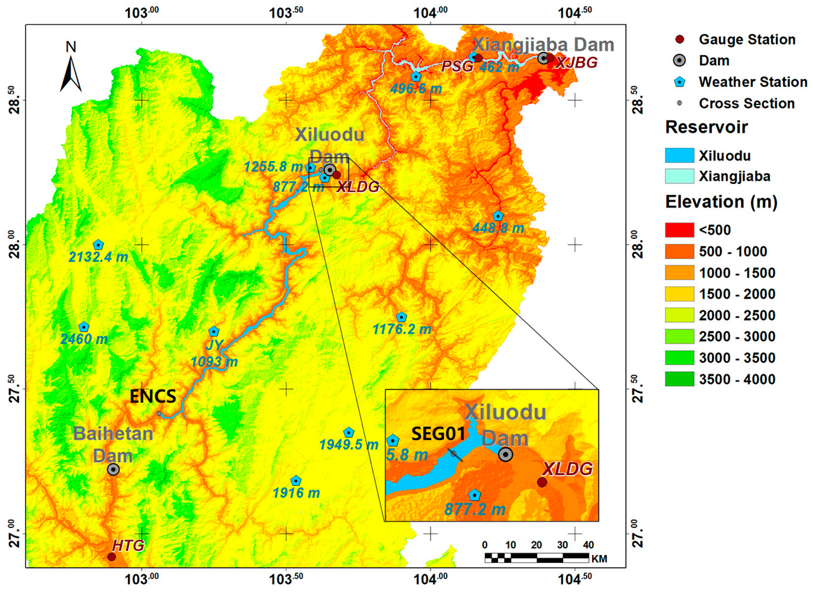
2.1. Study Site

XLDR is the third reservoir of the four cascade reservoirs along the lower reach of the Jinsha River in the southwest of China; its surrounding topography is shown in Figure 1. These four cascade dams and reservoirs are mainly designed to generate hydropower. Other functions include flood control, sediment control, and improving river-shipping conditions. The dam of the Baihetan Reservoir, the second of the four, is supposed to be entirely constructed in 2022 and will be 197 km (when referring to the distances between different sites in a river, the distances are following the river meanders) upstream from the dam of XLDR. The dam of the Xiangjiaba Reservoir (XJBR, Figure 1 and Table 1) is 147 km downstream from the dam of XLDR.
The Xiluodu hydropower complex consists of a concrete hyperbolic arch dam, flood releasing structures, and power-tunnels leading water to huge underground powerhouses on both sides of the river. The top elevation of the dam is 610 m above sea level (a.s.l.), and the elevation of the riverbed near the dam is 360 m a.s.l. In the Xiluodu dam, there are eight 10.5-m deep outlets at the elevation around 495 m a.s.l. On both sides of the river, there are nine 10-m high and 8-m wide power-tunnels with the entrance bottom elevation at 518 m a.s.l., and two 15-m high and 10-m wide flood-tunnels with the entrance bottom elevation at 545 m a.s.l.
The basin of XLDR is a typical canyon-shape, and the slope of the riverbed is around 0.11%. The length of the reservoir is about 155 km where the water surface is near horizontal and surface width varies from 150 to 1000 m. The water depth near the dam ranges from 180 to 240 m throughout the year. The full storage (V) of XLDR is 12.3 km3, and it releases about 126 km3/year (Q) of water downstream. The large storage with small hydraulic residence/detention time (td = V/Q = 0.1 year = 37 days) distinguishes XLDR from other reservoirs. Typically, small td is for small V while large td is for large V.
The impoundment of XJBR was initiated on 10 October 2012. The water elevation dramatically increased from 280 to 354 m a.s.l. within 6 days due to the large inflow, stayed around 354 m a.s.l. until 8 June 2013, the beginning of the flood season, and then reached the minimum operating water level 370 m on 5 July 2013. The impoundment of XLDR was initiated on 4 May 2013 when water elevation was 440 m a.s.l. and water depth was 80 m. The water level reached the minimum operating water level 540 m a.s.l. on 23 June 2013, storing 4.7 km3 of inflow within 50 days.
XLDR is located in a subtropical valley, and its annual minimum surface temperature is above 11 °C. The study area is the impoundment area of XLDR, 155 km long upstream from the dam of XLDR. The ratio of reservoir length to maximum water depth is over 580, and the ratio of surface width to water depth is between 2.2 and 11.3. The entrance cross-section (ENCS, Figure 1 and Table 1) of XLDR is relatively shallow (8–48 m) and vertically uniform or weakly stratified. The middle and lower reach of XLDR is deep enough to maintain stable thermal stratification from April to December. The reservoir has attributes similar to a warm monomictic lake but is distinguished from others by its magnitude of the inflow and outflow.

2.2. Observed Water Temperatures

The vertical temperature profiles at the middle of SEG01 (the cross section 3.5 km upstream to the Xiluodu Dam in Figure 1 and Table 1) were measured in September and December 2013 and every month in 2014, using a profiler (HY1200B, Wuxi, China). The measured temperature, along with the simulated temperature, will be discussed in Section 3.2 for model calibration.
The surface temperature was obtained at 8 a.m. near the shore at four gauge stations (HTG, XLDG, PSG, and XJBG in Figure 1 and Table 1) from 2000 to 2014. The water depths are relatively shallow with high longitudinal velocity, so temperature is nearly uniform over the cross sections due to sufficient mixing. At the downstream of the Xiluodu dam, the Xiluodu gauge station (XLDG) measures the temperature of well-mixed outflows through all the outlets and tunnels of XLDR from January 2012 to December 2014, except from July to December 2013, when a landslide interrupted the data collection. The Pinshan gauge station (PSG) was 29.5 km upstream of XJBR dam, and the water temperature was measured there from 2000 to 2011. At the end of 2011, it was abandoned since it would be submerged into XJBR. As an alternative, the Xiangjiaba gauge station (XJBG) was set up at the section 2 km downstream of the Xiangjiaba dam, to measure the fully mixed temperature of outflows from XJBR. Temperatures at PSG and XJBG were treated as one continuous time-series from 2000 to 2014.
Since the diurnal fluctuation of water temperature generally reaches its daily minimum at sunrise [7,50], the temperature measured at 8 a.m. is typically smaller than the daily average temperature. We used the long-term observed hourly temperatures in the Tallapoosa River (Alabama, USA, data obtained from the U.S. Geological Survey’s website), which is at a similar latitude (32°28′ N) to XLDR (27°50′ N), to estimate the difference of temperatures between at 8 a.m. and the daily average. The data from 2007 to 2017 in the Tallapoosa River show that daily average temperatures in different seasons are about 0.1 to 1.2 °C higher than the temperatures measured at 8 a.m. In this study, daily average temperatures at ENCS (inflow for XLDR, see Figure 1) were used as input data for the XLDR model and were estimated from measured temperatures at 8 a.m. at HTG plus different increments of temperature in different seasons. Through a trial-and-error sensitivity analysis, the temperature increments were determined when the simulated temperature profiles at SEG01 matched the measured vertical profiles better, and the average calibrated increments were 0.19 ± 0.90 °C. For other comparison and analysis of temperatures at different gauge stations, the temperatures measured at 8 a.m. were used in this study.

2.3. Two-Dimensional Simulation Model

CE-QUAL-W2 (W2), developed by the U.S. Army Corps of Engineers, is a two-dimensional, laterally averaged, hydrodynamic and water quality model. It has been widely applied to long and narrow reservoirs [40,41,42,51,52,53]. It was used in this study to enhance the understanding of the thermal structure of XLDR by simulating more details of spatial and temporal temperature variations under real boundary conditions from May 2013, which was the month of XLDR’s impoundment, to December 2014, after which not enough input data were available to support further model simulation.
The vertical temperature profiles measured once from different vertical lines along SEG01 show that those temperatures were identical at the same depth along the section. These characteristics imply that the laterally averaged hydrodynamic model W2 is suitable for XLDR.
Bathymetry of the W2 model for XLDR was built based on 163 measured cross-sections including underwater topography. The computational domain is 155 km long starting from ENCS and ending at the Xiluodu Dam (Figure 1). The riverbed elevation at the upstream ENCS is 532 m a.s.l., just 8 m below the lowest surface elevation of XLDR, where the temperature distribution is sectional uniform according to the observation from 2013 to 2014. The W2 model developed for XLDR has 201 segments of 500-to-800-m long in the longitudinal direction and 249 layers 1 m thick in the vertical direction.

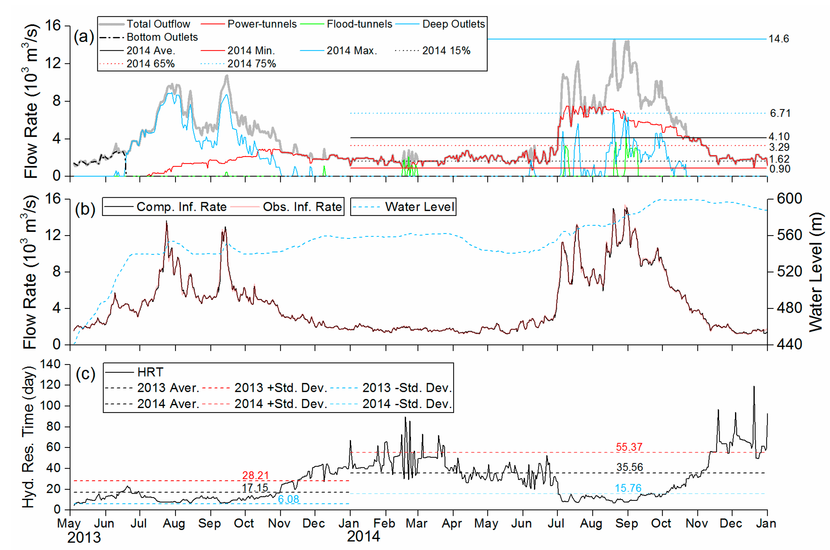
2.3.1. Hydrometric Input Data

Measured outflows through tunnels and outlets and computed daily average inflow at ENCS from May 2013 to December 2014, varied seasonally with maximal values from June through September (Figure 2a,b). The daily average inflow was measured at HTG (Figure 2b), but in this study, the inflow at ENCS was computed using the measured water level, outflow, tributary inflows, evaporation and precipitation, and the level-volume relationship of XLDR. The water surface elevations were measured four times a day near the dam, and all these data came from the reservoir operator. The computed inflow time-series matched well with observed inflow (Figure 2b). The annual average of daily inflow observed at HTG in 2014 was 4209 m3/s while the annual average of the computed inflow at ENCS was 4193 m3/s, and the percentage difference was 0.35%. In XLDR, there are four small seasonal tributaries flowing into the reservoir during rainy days, and the total tributary inflows and seepage through river banks are very low compared with measured inflow at HTG. Therefore, tributary inflows and seepage were incorporated into the adjusted upstream inflow in this study, neglecting their contributions at specific locations in the model for XLDR.
Upstream inflow (Figure 2b) varied seasonally and the inflow in the flood season (from July to September) contributed about 53% to the annual inflow. In the flood season, the water was discharged downstream through the deep outlets, flood-tunnels, and power-tunnels, while water mainly went through power-tunnels in non-flood seasons (Figure 2a). In 2014, about 85% of the total outflow was used for power generation. In 2013, XLDR’s water level didn’t reach the maximum operating water level of 600 m at the end of flood season for security reasons and reached the maximum elevation in 2014 (Figure 2b). In 2014, the surface elevation of XLDR remained between the minimum operating water elevation (540 m) and the maximum operating water elevation (600 m).

2.3.2. Meteorological Input Data

Daily weather data, including near-ground air temperature (°C), ground temperature (°C), humidity (%), wind speed (m/s), and wind direction were measured at 11 weather stations (Figure 1) in the region surrounding XLDR from 2000 to 2014. The Jinyang weather station (JY in Figure 1 and Table 1), located near the middle of XLDR, gives representative weather conditions over the impoundment area of XLDR. Elevations of these 11 stations vary from 448 to 2460 m a.s.l., but the reservoir water surface elevation is about 540–600 m a.s.l. Therefore, weather data at JY (1093 m a.s.l.) were adopted and adjusted for the XLDR W2 model.
No measurement of shortwave radiation was available in the XLDR region, and the average of daily shortwave radiations measured at two nearest radiation stations (one is ~200 km in the northeast, and the other is ~200 km in the southwest of XLDR) was used for the XLDR model in 2013 and 2014. Cloud covers were estimated by the ratio between measured shortwave radiation and the theoretical maximum under the cloudless condition in this area. Precipitation data at JY in 2013 to 2014 were adopted in this study and ground temperature at JY was used as precipitation temperature.
Air temperatures in mountainous areas are strongly correlated to elevation [54,55,56,57,58]:
d T a i r d z = k ,
where k (°C/100 m) is the lapse rate to quantify the air temperature decrease with the increase in altitude (elevation z). The value of k changes diurnally and seasonally and varies with topography, longitude, and latitude [54,55,56,57,58]. Through linear regressions of air temperatures from 11 weather stations around XLDR we obtained good estimations of k with average R2 of 0.94 for a whole year (Table 2). Then, air temperatures at JY were adjusted to the elevation of 580 m using Equation (1) and monthly k in Table 2, as better estimations for the surface air temperatures in XLDR. The annual average of the original air temperatures at JY in 2014 was 17.47 °C and of the adjusted temperatures was 19.53 °C. Dew point temperature (°C) was calculated based on the relative humidity and the adjusted air temperature using the method of Arden Buck [59,60].

2.4. Annual Temperature Variations

The water temperature ( T w ) variation in a river consists of a periodic seasonal variation ( T A ) and a short-term non-seasonal fluctuation ( R W ) [39,61,62,63,64,65]:
T w = T A + R W ,   T A = a + b × sin ( 2 π t + c 365 ) ,
where T A (°C) is the seasonal change of water temperature over a year, R W (°C) is the departure of water temperature from the seasonal trend due to the short-term air temperature variations and other disturbances, t is day of year or Julian day (1 January is t = 1 and 31 December is t = 365 for a non-leap year and t = 366 for a leap year), and a , b , and c are the regression coefficients. To be specific, a (°C) is similar to the annual average temperature, b (°C) is the amplitude of annual temperature variations, and c is the phase shift in days in order to evaluate the phase delay between outflow and inflow more intuitively.
The seasonal variation of temperature before and after the impoundment was our main concern in this study, and the short-term fluctuation was not studied further because this part was relatively small local deviation of temperature from the annual trend. For the seasonal variation, the fitted coefficients a , b , and c were calculated by optimizing the sine function of temperature time series in Equation (2) against observed temperature over a year with the least-square-error method.
In this study, we mainly concerned the phase difference of the temperature time series in each year between inflow and outflow as well as the phase difference at a given cross-section under different inflow conditions. The seasonal variation of outflow temperature in many large dams was delayed in comparison to their inflow temperature [5,7,9]. We referred to this change in annual temperature variation as phase delay here, and the differences of c between outflow and inflow were used to describe the levels of delay quantitatively.
The mean absolute error (MAE) and the root mean square error (RMSE) were adopted to evaluate the goodness of the fitted temperature curve, as well as the differences between observed temperatures and simulated temperatures, and they were calculated as:
M A E = 1 n i = 1 n | T s i m i T o b s i |
R M S E = i = 1 n ( T s i m i T o b s i ) 2 n ,
where T s i m i is either the fitted or the simulated temperature, T o b s i is the observed temperature, and n is the number of pairs of temperature data on annual temperature time series or a vertical profile with 1 m interval.

2.5. Hydraulic Residence Time and Water Age

Hydraulic residence time (days) is defined as the volume of a reservoir divided by its outflow rate, and the value indicates that, on the scale of the entire reservoir, how long the outflow needs to replace all the water or how long the water will stay in the reservoir at the outflow rate.
Water age (days), which is slightly different from the local hydraulic residence time, depicting the duration of time that water has stayed in a waterbody, is defined as the persistence of water after it enters a reservoir from upstream [66,67,68,69]. In the XLDR W2 model, we set a virtual constituent as a state variable that has an initial value of 0 entering the reservoir; it decays by 1 per day and does not interact with any other water quality state variables. This variable represents water age [40]. By using water age, we can identify the transport of the inflow water and the corresponding mixing processes. The water age of new water flowing into the reservoir is always less than the age of the ambient water already in the reservoir. For instance, in the case of overflow in a reservoir, the fresher water in the upper layer has a lower water age than the ambient water in the lower layers.

2.6. Definition of Stable Stratification

We quantified thermal stratification by setting thresholds to identify the epilimnion, metalimnion, and hypolimnion. Vertical temperature gradient (VTG, °C/m) and buoyancy frequency (N, 1/s, converted to 1/h or cph) were calculated based on temperature profiles observed at SEG01 (Figure 1):
V T G = T ( z ) z
N = g ρ 0 ρ ( z ) z ,
where T(z) is the water temperature (°C) at depth z (m), ρ ( z ) is the water density (kg/m3) at depth z, which is the function of temperature [40], ρ 0 is the average water density of whole water column, and g is the gravitational acceleration (9.8 m/s2).
Though N is the convention in limnology and oceanography, the variation trends of vertical temperature gradient and N were similar, and both can distinguish vertical layers by setting the corresponding thresholds. The temperature gradient and N are not in a linear relationship based on Equations (5) and (6). Finally, we chose the vertical temperature gradient as the threshold because it was more intuitive than N.
The vertical temperature gradient in the hypolimnion was reported to be very small [70] with a magnitude of 0.001 °C/m. In the epilimnion it may have slight variations with time (unsteady) due to its high dependence on atmospheric conditions, but with an average of 0.01 °C/m. The metalimnion is recognizable by its larger temperature gradient. In this study, the vertical temperature gradient was firstly calculated from measured temperature profiles at SEG01, and then a threshold was selected to identify the metalimnion, i.e., the water layer with a temperature gradient higher than the threshold was regarded as the metalimnion. From April to September, the surface heating can create a thin surface layer where the temperature gradient can be higher than the threshold, but it is neither stable nor continuous. This surface layer is known as the diurnal thermocline [17] and is a component of the epilimnion. The threshold used to identify the metalimnion in the observational data was applied to the simulated temperature profiles from the W2 model. The period of stable stratification was defined as the time with stable metalimnion that was continuous spatially and temporally.

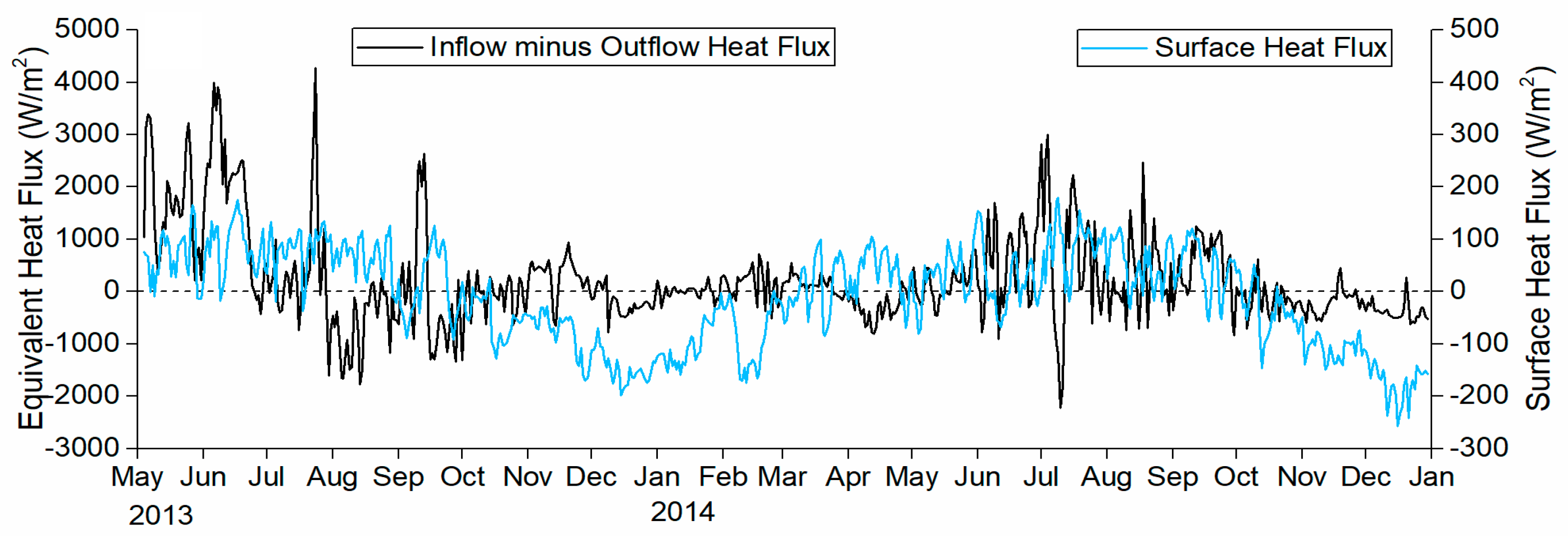
2.7. Equivalent Heat Flux of Inflow and Outflow

We transferred the heat contained in inflow and outflow to an equivalent heat flux, which had the same unit as surface heat flux, normalized by the reservoir surface area:
q i n = T i n Q i n ρ C p A
q o u t = T o u t Q o u t ρ C p A ,
where q i n and q o u t are the equivalent heat fluxes (W/m2) of inflow and outflow, T i n and T o u t are the temperatures (°C) of inflow and outflow, Q i n and Q o u t are the inflow and outflow rates (m3/s), ρ is the density (1000 kg/m3) of water, C p is the heat capacity (J/K/kg) of water, and A is the surface area (m2) of the reservoir. After being normalized by the surface area, these heat fluxes through inflow and outflow can be compared with the heat flux through the water surface due to solar radiation and atmospheric exchange over the simulation period.

3. Results and Discussions

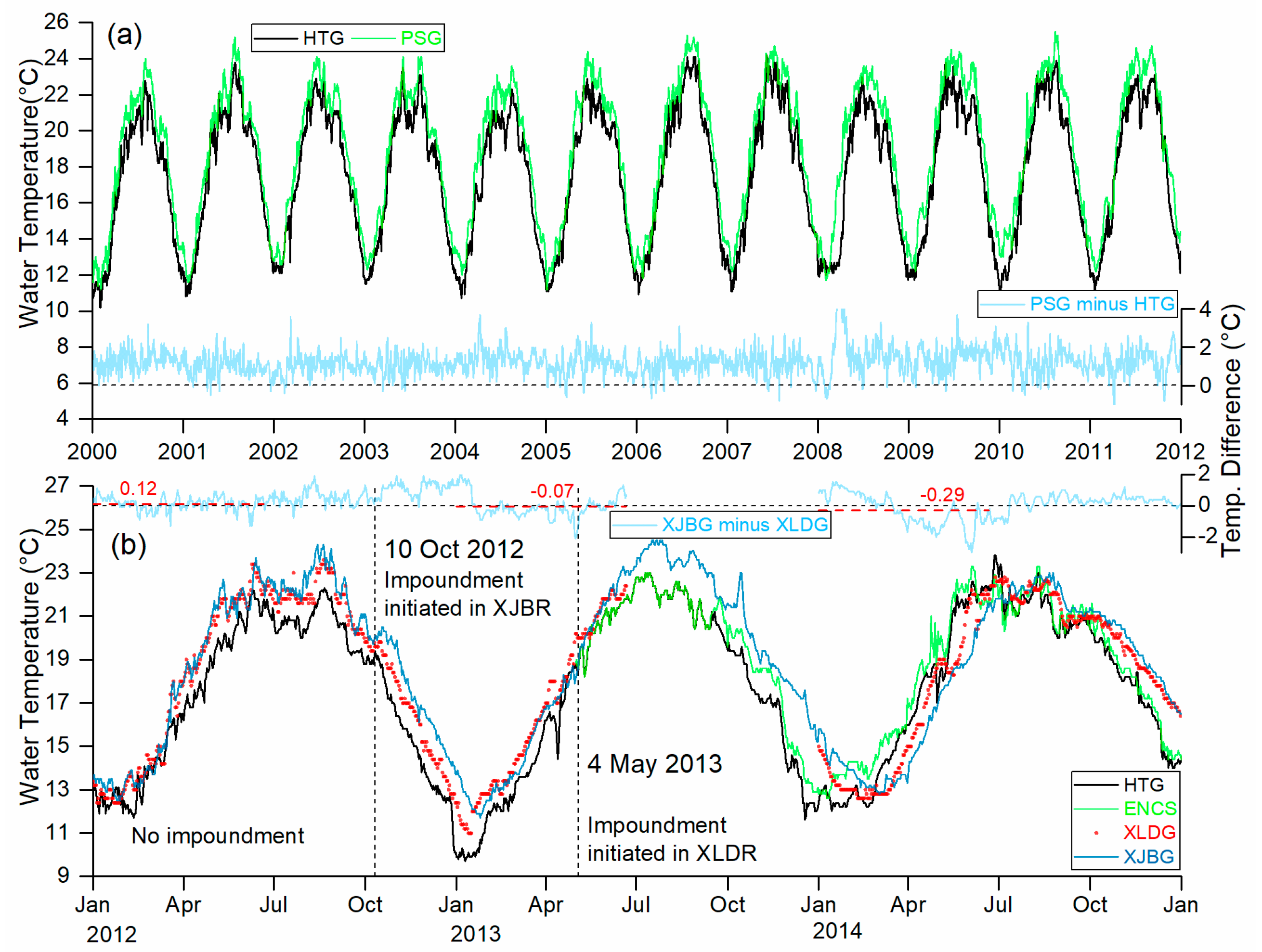
3.1. Annual Temperature Variations before and after Impoundment

3.1.1. Temperature before Impoundment

Daily temperature data for each year from 2000 to 2014 (Figure 3), as well as daily average air temperature at JY, were fitted using Equation (2) to identify the seasonal variation. Annual average temperatures at HTG and PSG were 17.61 ± 0.46 °C and 18.82 ± 0.42 °C from 2000 to 2011, respectively. Therefore, prior to the impoundments of XJBR and XLDR, the average temperature differences between PSG (353 km downstream) and HTG were 1.21 ± 0.66 °C from 2000 to 2011 (Figure 3). Thus the longitudinal temperature gradient was 0.0034 °C/km, less than the typical value of 0.2 °C/km for intermediate rivers [7]. The average amplitudes of the annual temperature fluctuation and the phase shifts at PSG were only 0.12 °C higher and 0.23 day longer than ones at HTG before the impoundment (Figure 4). Therefore, before the impoundments of XJBR and XLDR, the differences of the fluctuation amplitudes and the phase delays between PSG and HTG are negligible, but the annual average temperature increase from HTG to PSG is not negligible even though it is not large.

3.1.2. Temperature after Impoundment

The average temperature difference between XJBG and HTG in 2014 was 1.06 ± 2.11 °C. The average temperature differences between XJBG and XLDG in the first half-year (January–June) of 2012, 2013, and 2014 were 0.12, −0.07, and −0.29 °C (Figure 3b). It seems the seasonal variations of temperatures at XLDG and XJBG were different in 2012 and 2014. Annual averages and amplitudes at XLDG and XJBG were basically the same in 2012 and 2014. The phase shift of the seasonal variation ( c in Equation (2)) at XJBG was −114.1 days in 2012, −126.3 days in 2013, and −144.5 days in 2014, where the phase shifts in 2013 and 2014 became quite different from the long-term (2000–2011) average phase shift of −110.2 days. At XLDG, the phase shift changed from −108.6 days to −133.9 days from 2012 to 2014. The negative c means shifting the normal sine function to the right (delaying the time of maximum temperature).
These phase shift changes at XLDG and XJBG were because of the phase shift change at HTG and the reservoir impoundment. The phase shift change at HTG (Figure 4: −108.5 to −117.4 days from 2012 to 2014) would respond to air temperature phase shift change or other unknown disturbances further upstream of HTG (Figure 4c). In 2014, the phase shift difference between HTG and XLDG was 16.5 days, and the difference between HTG and XJBG was 27.1 days (Figure 4c). These phase shift differences were no longer negligible. The inflow of XJBR is the release from XLDR, and there is no natural river between them. Impoundment led to phase delays of water temperature in the heat release from a single reservoir like XLDR or XJBR. When flow went through more than one reservoir, as with XLDR and XJBR, the final heat release from the downstream reservoir (XJBR) was further delayed, compared with the heat release from the upstream reservoir (XLDR). Besides, the annual average temperature at XJBG turned to be only 0.3 °C higher than that of HTG, which was supposed to be 1.21 °C higher downstream before impoundment (Figure 4a).
Though not referred to as the phase delay, the phenomenon of the annual temperature of outflow shifting rightward compared with inflow or at the control site is widely observed and discussed in many studies about reservoir outflow temperatures. The changes from inflow to outflow could be described as the combination of phase delay, the decrease of annual average temperature as well as reduction of annual fluctuation amplitude or only part of them [3,5,7,49,71,72,73]. However, XLDR has a much larger flow rate than most of the reservoirs in previous studies, and it displays a major change as the phase delay.

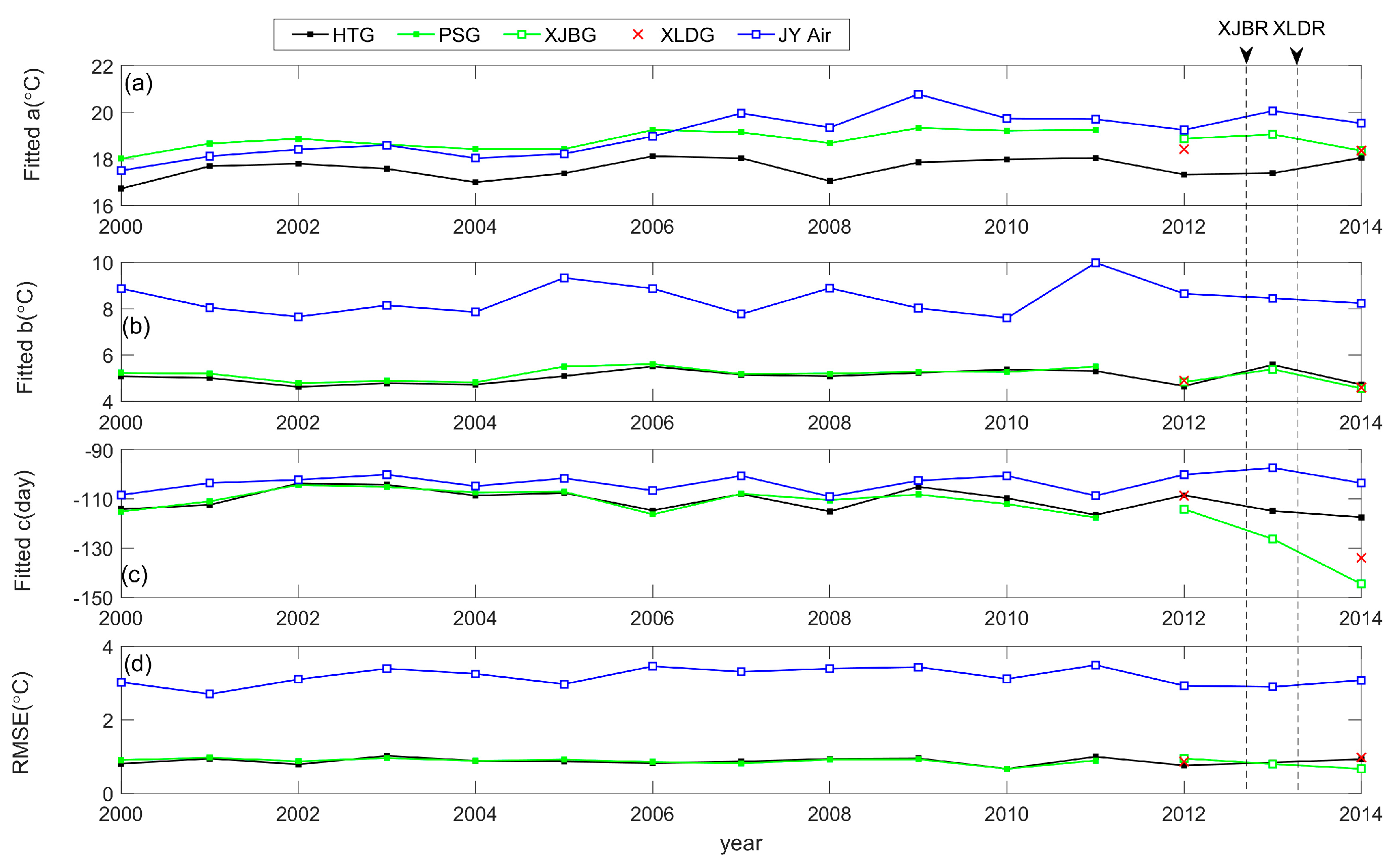
3.1.3. Relationship between Air and Water Temperature

For shallow rivers, various studies have demonstrated that there are strong correlations between the air temperature and water temperature. Historically, various empirical regression equations were developed to estimate river temperatures using air temperatures in hourly, daily, weekly, monthly, and annual time steps [62,63,74]. The annual average air temperature of JY had similar fluctuation trend as the river temperature of HTG where the water was nearly vertically uniform, but the difference between them increased after 2006 (Figure 4a). Their average temperature differences were 0.8 and 2.1 °C while their correlations were 0.90 and 0.46 for 2000–2006 and 2007–2014, respectively. The linear regression of annual air temperature shows a warming rate of 0.16 °C/year with R2 of 0.62. For the phase shift c ((Figure 4c), the average c value of air temperature at JY from 2000 to 2014 was −103.3 ± 3.4 days, and the c value in 2014 was −103.5 days that stayed in the range of the historical fluctuation. There seemed to have no dramatic change of the air temperature’s phase shift before and after the reservoir’s impoundment.
However, the phase shift difference between the air temperature and the water temperature at PS/XJB increased to 28.9 days in 2013 and 41.1 days in 2014, from the average difference of 6.8 days during 2000–2012 (Figure 4c). This discrepancy of the phase shift indicates that the variation of air temperature was not the reason that leads to the temperature phase delay after the impoundment.

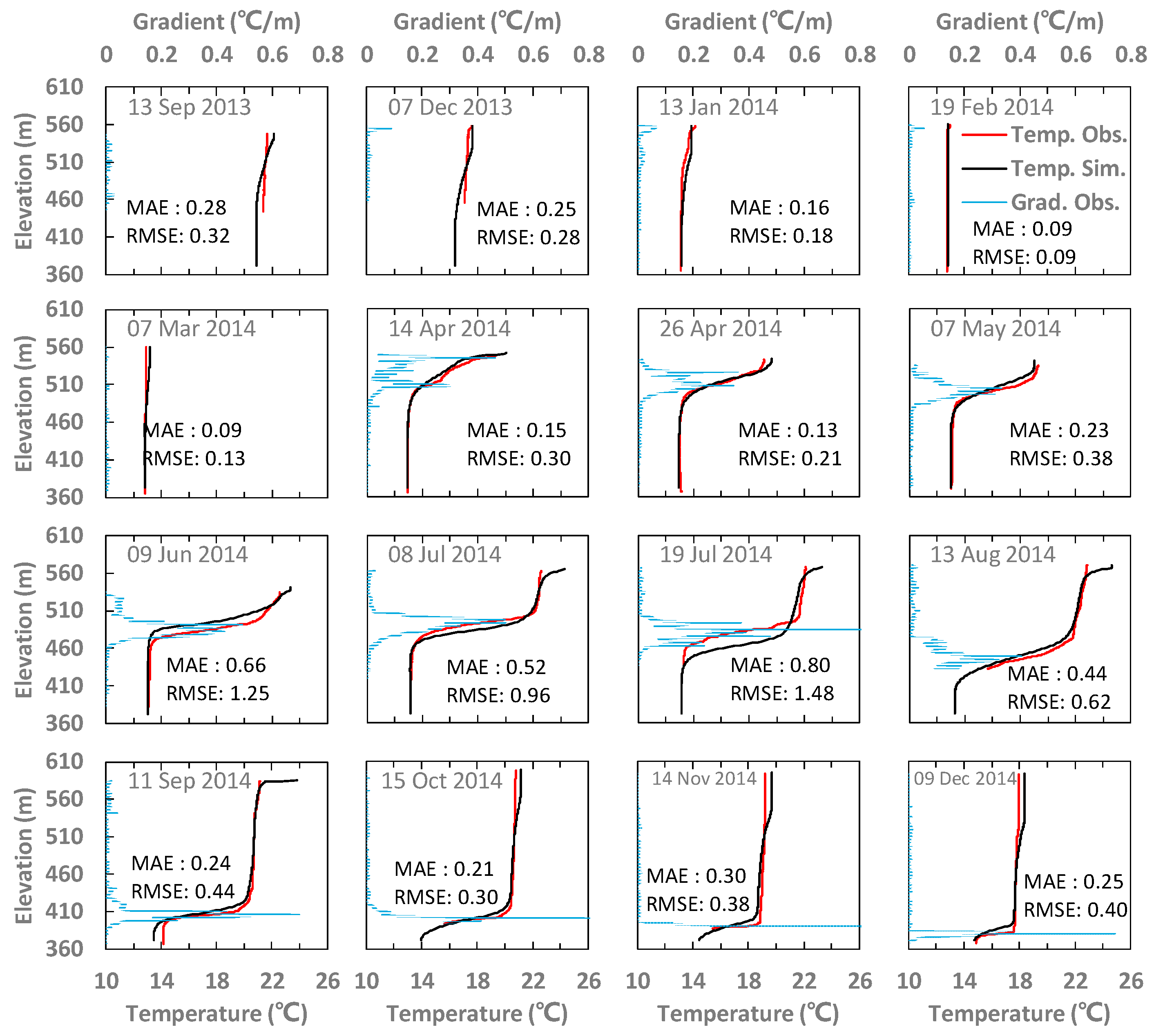
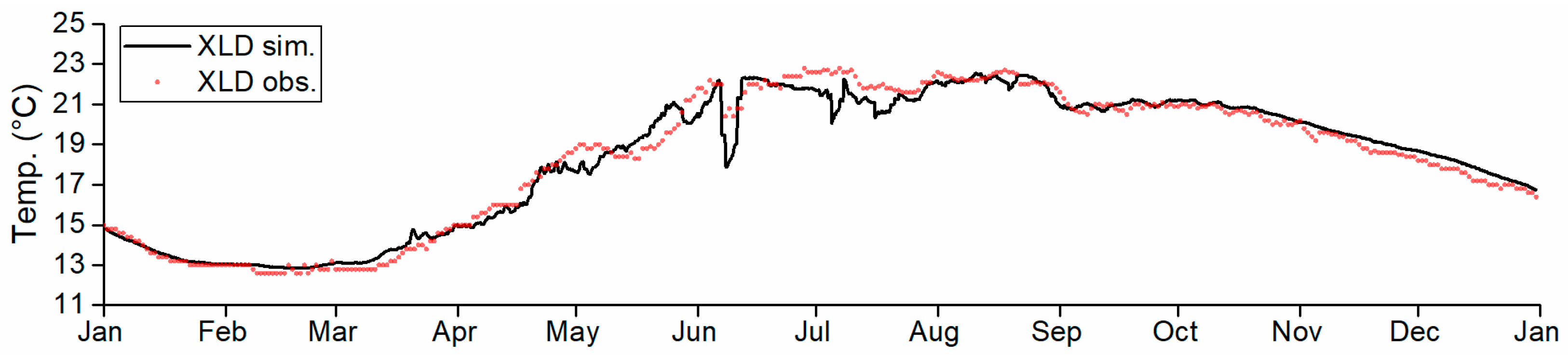
3.2. Xiluodu Reservoir (XLDR) Model Calibration

The calibration of XLDR’s W2 model focused on several critical coefficients that had the greatest influence on the simulated temperature profiles at SEG01. The inflow at ENCS was computed based on observed water surface elevation, so the calibration of the simulated water surface elevation was not necessary.
The critical model parameters are the shading coefficients (the ratio allowing incident shortwave solar radiation to reach water surface in different segments due to the topographic shelter), the horizontal dispersion coefficients for momentum (Ax) and the temperature/constituents (Dx). The XLDR is sheltered by mountains, and since the solar altitudes vary with season, the shading coefficients could be larger in summer and smaller in winter in XLDR. However, due to the lack of direct measurement of the solar radiation near the reservoir surface, a constant shading coefficient was used in the whole year for the XLDR W2 model. The sensitivity analysis indicates a value of 0.6 for the shading coefficient was able to generate simulated temperature profiles with minimal discrepancy from the observations.
The values of Ax and Dx are often set as the same but vary depending on the wind, water depth, vertical shear, bottom topography, and basin morphometry [75]. Fischer et al. indicated the horizontal dispersion in rivers and estuaries ranged from 0.1 to 1500 m2/s [76]. A series of sensitivity analyses on horizontal dispersion coefficient was conducted for the model. Prior to the flood season, the thermal structure was well simulated regardless of the value of Ax selected. Afterward, the simulated temperature profiles at SEG01 matched well with observations when Ax = 230 m2/s (Figure 5) and ultimately this value was adopted for the model.
The vertical dispersion coefficients for momentum (Az) and temperature/constituents (Dz) were calculated by the W2 closure scheme, which includes the effects of cross-shear from wind and has been successfully applied to many stratified reservoirs [40]. The light extinction coefficient was 0.85 m−1 determined from the measured Secchi depth (2 m). Other coefficients including the coefficients for wind sheltering and for the riverbed friction were set as default or recommended values based on the reservoir type; the sensitivity analyses showed that the default or recommended values worked fine.
The calibrated W2 model was able to simulate the temperature profiles near the dam (Figure 6) and the outflow temperatures (Figure 7) to a reasonable accuracy. The average MAE of all the 16 measured profiles was 0.30 °C, and RMSE was 0.50 °C, while MAEs of June and July were higher (Figure 6) when the occurrence of flood peaking (Figure 2b) rapidly deepened the epilimnion. The simulated outflow temperatures (Figure 7) in 2014 matched well with the observed temperatures at XLDG, with the MAE of 0.41 °C and the RMSE of 0.57 °C. The discrepancies between simulated and observed SEG01 profiles, as well as outflow temperatures, were partly contributed by the inaccuracy of simulated deepening of the epilimnion in June and July, when the simulated deepening was faster than the observed deepening.

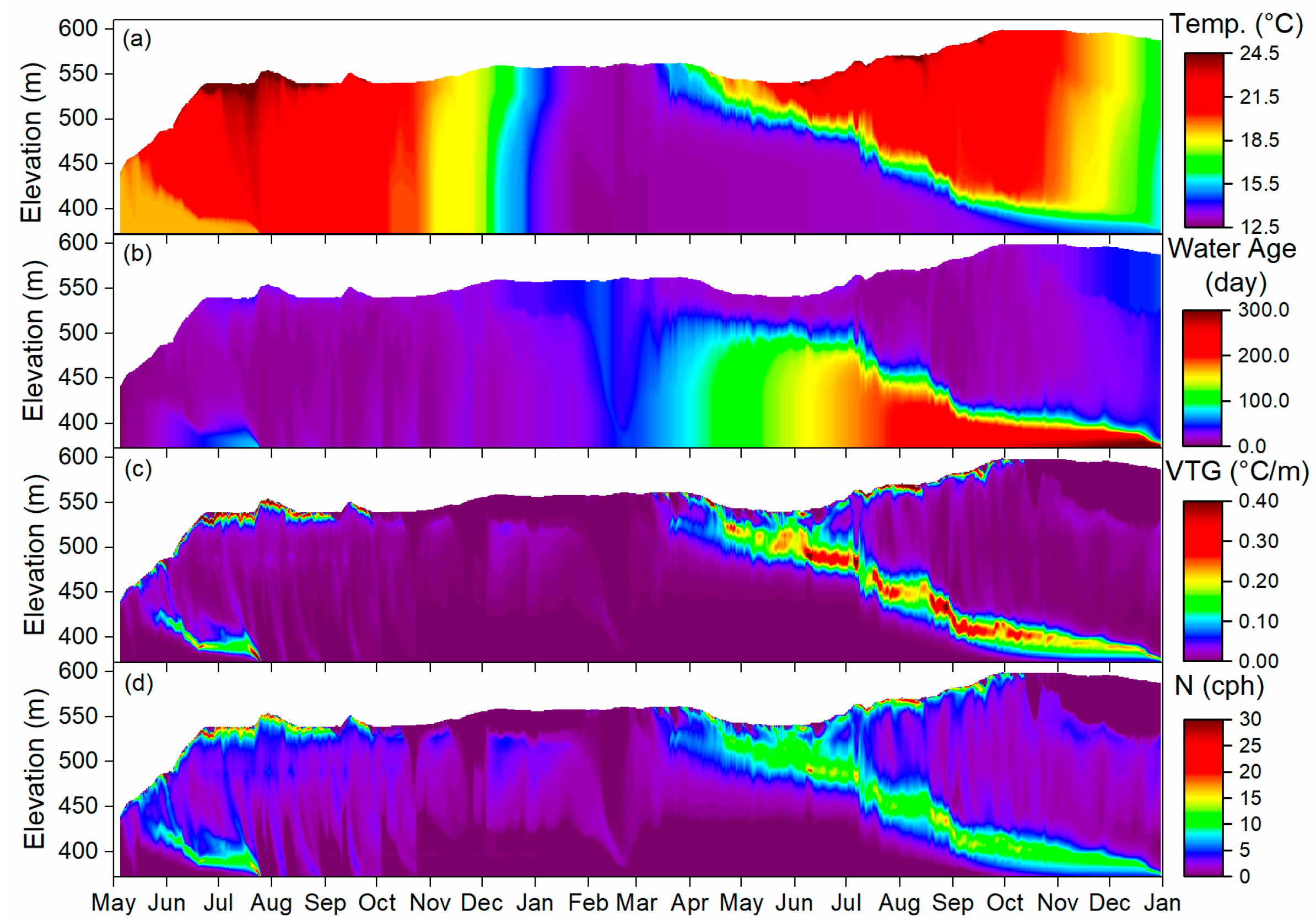
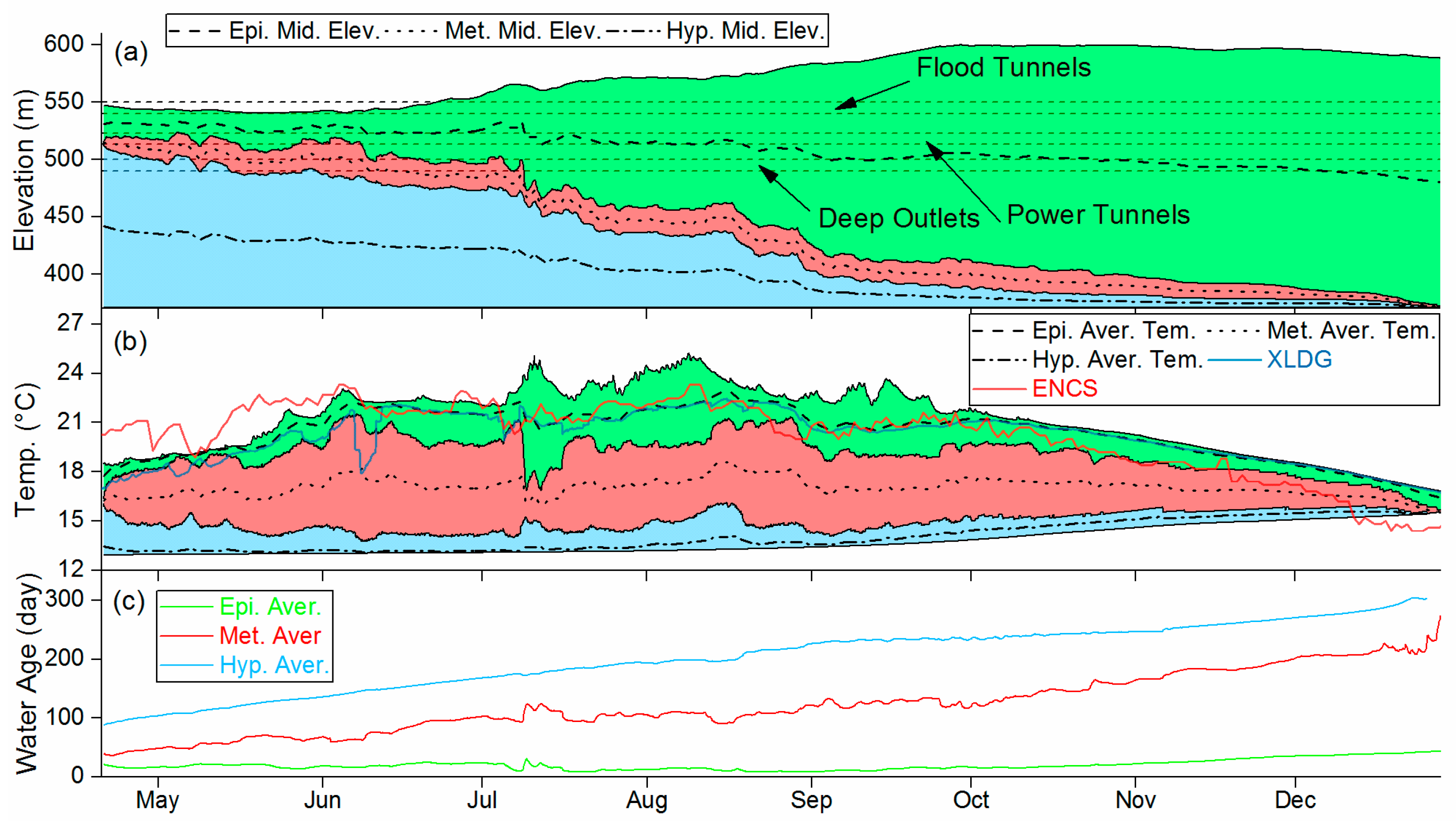
3.3. Thermal Structure in Xiluodu Reservoir (XLDR)

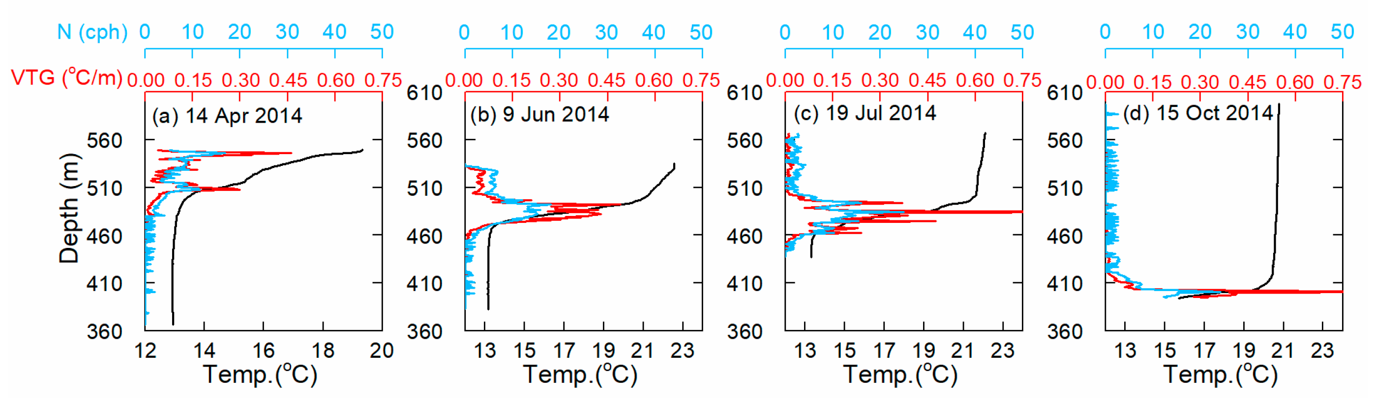
3.3.1. Thresholds of Vertical Temperature Gradient and N for Stratification

The temperature stratification first appeared in late May 2013 when the epilimnetic temperature was around 21.5 °C while the hypolimnetic temperature was around 19.0 °C (Figure 8a). It could be identified by the higher vertical temperature gradient or N (Figure 8c,d). The vertical temperature gradients at the top and bottom interfaces of the metalimnion changed rapidly, about 0.1–0.2 °C/m (Figure 6). In this study, both temperature gradient and N were presented, and the gradient of 0.15 °C/m was adopted as the threshold identifying the metalimnion. The water layer with the gradient higher than 0.15 °C/m was regarded as the metalimnion, not including the diurnal mixing layer near the water surface. The corresponding N is about 10 cph at the temperature gradient threshold of 0.15 °C/m (Figure 9), which is moderately stratified. The temporal and spatial (along with depth) distribution of the calculated gradient and N at SEG01 demonstrated the ranges and variations of the epilimnion, metalimnion, and hypolimnion (Figure 8c,d). Under the stable stratification, XLDR’s gradients in the epilimnion and hypolimnion were tiny, on the order of 0.001 and 0.01 °C/m, respectively. During the stratification period, when the surface heat flux was positive (Figure 10), a thin layer on the surface was heated up, and the corresponding gradient and N were notably larger than ones in the epilimnion (Figure 8c,d or Figure 11e). This thin layer was not stable and highly depended on the surface heat flux.

3.3.2. Stratification in the First Year of Impoundment

The tremendous momentum of the upstream inflow created a well-mixed condition even at SEG01 (Figure 8a) at the early stage of impoundment in 2013, and a short period of weak stratification in XLDR occurred in June–July 2013 (Figure 8a). The water age of the epilimnion (7–15 days) was much smaller than that of the hypolimnion (40–80 days) during this period (Figure 8b), due to the warmer and lighter inflow flowed over the ambient water and then gradually mixed with the hypolimnion. Judging from the vertical distributions of the temperature, water age, temperature gradient, or N (Figure 8a–d), the metalimnion appeared on 29 May and disappeared on 26 July 2013, with an average deepening speed of 0.86 m/day. From the disappearance of the first stratification at the end of July 2013 to March 2014, the temperature at SEG01 developed from weakly stratified to vertically uniform, and the average temperature at SEG01 decreased from 22 to 13 °C (Figure 6 or Figure 8a).
The hydraulic residence time of the entire reservoir was calculated daily from the onset of impoundment on 4 May 2013 to 31 December 2014 (Figure 2c). The average hydraulic residence time from May to December 2013 was 17.2 days. The minimum value from June to October was 6.8 days when the outflow was ~10,000 m3/s at the water level ~552 m a.s.l. The maximum value in November and December was 44.2 days when the outflow was ~1800 m3/s, and the water level was near 560 m a.s.l.
The formation of the weak stratification was due to the colder and denser ambient water trapped by the warmer and lighter inflow water. Because the outflow was mainly drawn above the hypolimnion, mixing seems to be the primary factor that gradually eroded the lower layer (the ambient water). Before the inflow became cold enough to plunge below the epilimnion, the deepening of the thermocline had already reached the bottom of the reservoir, which marked the destruction of stratification in 2013.

3.3.3. The Weak Stratification Period

In SEG01, the temperature at 10 m below the surface (avoiding the influence of diurnal thermocline) was at least 0.2 °C higher than the bottom temperature on 7 December 2013 (Figure 6). On 13 January, 19 February, and 7 March 2014, the corresponding temperature differences were 0.66, 0.01, and 0.05 °C, respectively (Figure 6). According to these measured profiles (Figure 6) and simulating temperatures (Figure 8a), the vertical temperature at SEG01 was weakly stratified from October 2013 to January 2014 and was nearly homogenous in February and the beginning of March 2014.
From 4 December 2013 to 27 January 2014, the water age of the bottom layer (~20 days) was smaller than the water age in the surface layer (~40 days) (Figure 8b or Figure 11b). This indicates the colder and denser inflow flowed under the ambient water as underflow (Figure 11a). On the interface of the underflow and the ambient water, the largest gradient was ~0.04 °C/m (Figure 8c), and the corresponding N was ~4 cph (Figure 8d).
The net heat flux of flows ranged from −2224.5 to 4417.8 W/m2 (average of 226.7 W/m2 and very large standard deviation of 908.7 W/m2) and was much larger than the surface heat flow ranged from −256.5 to 180.5 W/m2 (average of −10.1 W/m2 and standard deviation of 91.2 W/m2) (Figure 10). This is because the difference between inflow and outflow was quite large and ranged from −2199.9 to 4487.8 m3/s (average of 173.3 m3/s and standard deviation of 767.9 m3/s) (Figure 2).
However, the surface heat flux and the net heat flux of flows were similar or had fewer differences in the winter and early spring of both 2013 and 2014 (Figure 10). During the period from 9 December 2013 to 30 January 2014, the surface heat flux was negative (−127 ± 42 W/m2). The surface heat transfer reduced the thermal energy of XLDR from the surface, producing convectional mixings and leading to incomplete overturn (Figure 8a). The equivalent heat flux of flow was basically negative (−142 ± 204 W/m2) during the same period, and of the same magnitude as the surface heat flux (Figure 10). The homogeneous inflow firstly pushed the ambient water forward [30,31,32], so the upstream water responded rapidly to the change of the reduction of inflow temperature (Figure 11a). When the inflow plunged somewhere beneath the ambient water, the underflow entrained with the ambient water [30,31,32] and cooled it down from the bottom (Figure 11a,b). The underflow created a colder and denser bottom layer, and this might be the reason why the overturn did not fully develop to the riverbed until February when the measured profile proved the vertical temperature was uniform at SEG01 (Figure 6). During this period, the equivalent heat flux, as well as the surface heat flux, was negative, reducing the heat of the reservoir water. After the middle of March, the surface heat flux grew from negative to positive, marking the transition from surface losing heat to absorbing heat (Figure 10).

3.3.4. The Stratification in the Second Year of Impoundment

The seasonal stratification with continuous temperature gradients equal to or larger than 0.15 °C/m started on 20 April 2014 and ended at the end of 2014 (Figure 12). At the beginning of this stratification, the warmer and lighter inflow water flowed over the ambient water and could be identified by its lower water age (Figure 8b). It is evident that the water age was much lower in the epilimnion than in the hypolimnion, from the entrance to the dam of XLDR (Figure 8b or Figure 11d,f). During the stratification, the metalimnion deepened at a rate of 0.49 m/day when the average inflow rate was 4447 m3/s. The flood peaks were highly related to the rapid deepening of the metalimnion. From 3 July to 28 July and 16 August to 9 September, when the inflows were above 7000 and 10,000 m3/s, respectively (Figure 2b), the metalimnetic deepening speeds were about 1.61 and 1.67 m/day (Figure 12a), respectively. When stratified, the differences of average temperature between the epilimnion and the hypolimnion slowly increased from 4.7 °C (18.1–13.4 °C) on 21 April to 9.1 °C (23.0–13.9 °C) on 15 August, and then decreased to 1.5 °C (17.0–15.5 °C) on 22 December (Figure 12b). These changes were mainly due to the inflow of the warm river water into the upper layers in summer and the cooler river water into the lower layers in winter (Figure 11). The thickness of the metalimnion at SEG01 was 19 ± 6.3 m in 2014, about four times the thickness of the metalimnion in 2013 (~5 m). The elevation of the metalimnion seemed to be constrained by the elevation of the power-tunnels since the upper edge of the metalimnion was near the elevation of the power tunnels at the beginning of the stratification (Figure 12a) and then deepened with time afterward. At the end of the stratification in 2014, the epilimnion almost reached the bottom of the reservoir, similar to the destruction of the stratification in 2013.
Under the low inflow (~2000 m3/s) on 2 January and 1 June 2014, the upper 30-to-40-km portion in XLDR from ENCS was typically not stratified, and under the high inflow (~8000 m3/s) on 2 August the upper 80-km portion of XLDR was not stratified due to the larger inflow momentum (Figure 11). When the inflow was low on 1 June (Figure 2b), the thickness of the epilimnion gradually decreased from the upstream reach to the downstream reach while the thickness of the metalimnion increased (Figure 11c). Under the high inflow on 2 August (Figure 2b), the thickness of the epilimnion was more or less constant, and the metalimnion was near horizontal in the longitudinal profile (Figure 11e). The colder water in the early months of the year flowed as an underflow or a density current into the bottom part of the downstream portion of XLDR (Figure 8 and Figure 11). After the stratification had started in early summer, the bottom water was shielded by the metalimnion, separated from the inflow, and then had a continuous increase in water age (Figure 8 and Figure 11).
The average hydraulic residence time of 2014 was 35.56 days, about twice that of 2013 (17.15 days) (Figure 2c). In July–September, it was less than 15 days, more or less the same in both 2013 and 2014 due to the high inflow and outflow. In other months, it was much higher and reached to 117 days in December (Figure 2c). The water age of the metalimnion and the hypolimnion went back to zero after the destruction of stratification. The average water age of the epilimnion during the stratified period was 19.9 ± 8.74 days (Figure 12c). This means on average the epilimnetic water spent ~19.9 days traveling from ENCS to SEG01, although part of it was entrained from the metalimnion or the hypolimnion. The average water age in the hypolimnion increased nearly linearly in 2014, from 87.7 days on 4 April to 304.4 days on 26 December (Figure 12c), with an average growing speed of 0.87 days per day, slightly less than the growing speed of the water age had there been no mixing (1 days per day). The average water age of the metalimnion also increased with time in 2014.
From 26 April to 28 September, the daily net heat flux of inflow/outflow and the surface heat flux were basically positive (435 ± 786 and 45 ± 56 W/m2, respectively; Figure 10); therefore, the reservoir was heating up. These values indicate that the increased heat in the reservoir was near 9 times larger due to the summation of the inflow and the outflow than due to the surface heat exchange with the atmosphere. Consequently, the inflow and the outflow were the dominant factors that mainly controlled the thermal structure in XLDR during this heating period. The period from September to October was the transition period when the heating process changed into the cooling process because both heat fluxes became negative.
Though the shape, height, elevation, and duration of the metalimnion in 2014 were quite different from 2013, the mechanisms of the forming of stratification and deepening of the metalimnion were similar. The influence of inflow and outflow was of great importance for the whole year in XLDR, especially in the flood seasons, when it was the dominant factor. The surface heat flux was the other major factor controlling the temperature structure in the non-flood seasons but was relatively less important in the flood seasons. Inferring from the thermal structure in 2013 and 2014, we summarized the probable annual water cycle of XLDR. The cold water stored in XLDR before April each year is vertically uniform or weakly stratified. As the inflow temperature increases and forms overflow, the cold ambient water is covered, or trapped, by the later inflow water, stays at the bottom, and forms the hypolimnion. While gradually being eroded by the epilimnion, the hypolimnion shrinks, and the water which is newly flowing into XLDR eventually replaces it at the end of the current year or at the beginning of the next year. As part of the water cycling, the new water of the current year also forms the stored water for the next year.

3.4. The Factors Involving the Formation and Variation of Stratification

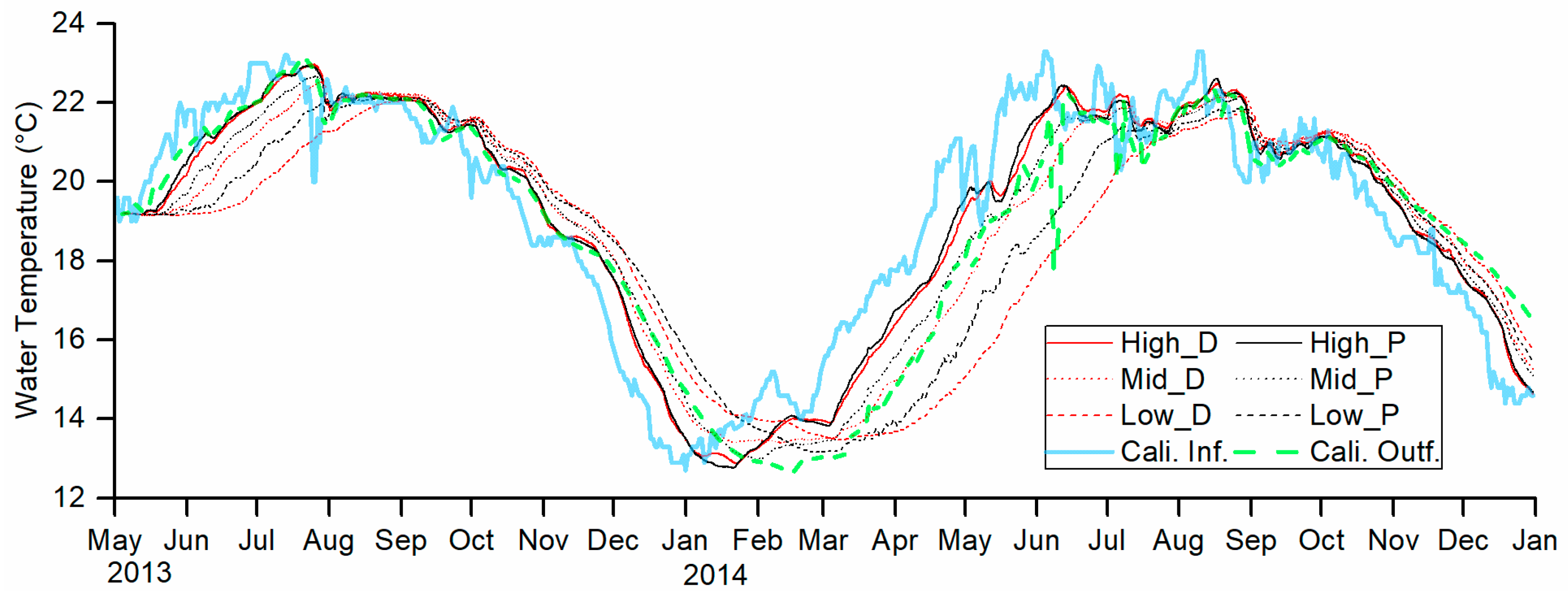
3.4.1. Scenarios Settings

Several factors such as inflow, outflows, and surface heat transfer could affect the formation of the stratification and the deepening of the metalimnion in XLDR. The outflows from XLDR were released primarily through the power-tunnels with the deep outlets as the supplement (Figure 2). XLDR was more like a deep running river rather than a typical lake having large hydraulic residence time. Six hypothetic model scenarios (Table 3) were developed to help us further understand how the inflow and outflow rates and elevation at which the outflow is withdrawn affect the variations of the thermal structure in XLDR. For instance, in the scenario with high outflow through the power-tunnels, the outflow rate (6710 m3/s) was in the 75th percentile in the outflow distribution curve of 2014 (the number of dates when outflow rates were equal to or less than 6710 m3/s accounts for 75% of the whole days in 2014). This outflow rate was set for every day, and all the outflow was withdrawn by power-tunnels with no outflow through the deep outlets. Inflows were the same as outflows to avoid the influence of water level fluctuation and the initial water level was 580 m a.s.l. These flow rates are within the maximal capacity of the power-tunnels or the deep outlets according to the records from 2013 and 2014 (Figure 2a). Other inputs and parameters of the W2 model stayed the same as the calibrated model. Of course, the inflow temperature is important and has significant influences on flow pattern (Figure 11a,c) [30,31,32], but they were not studied here.

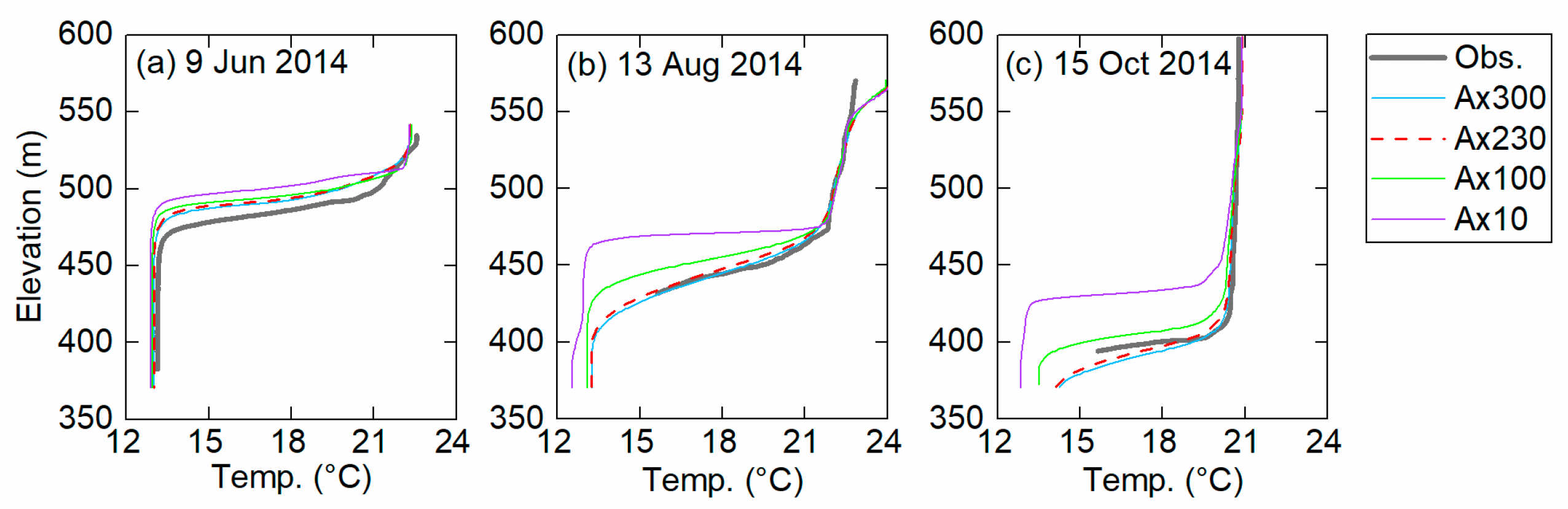
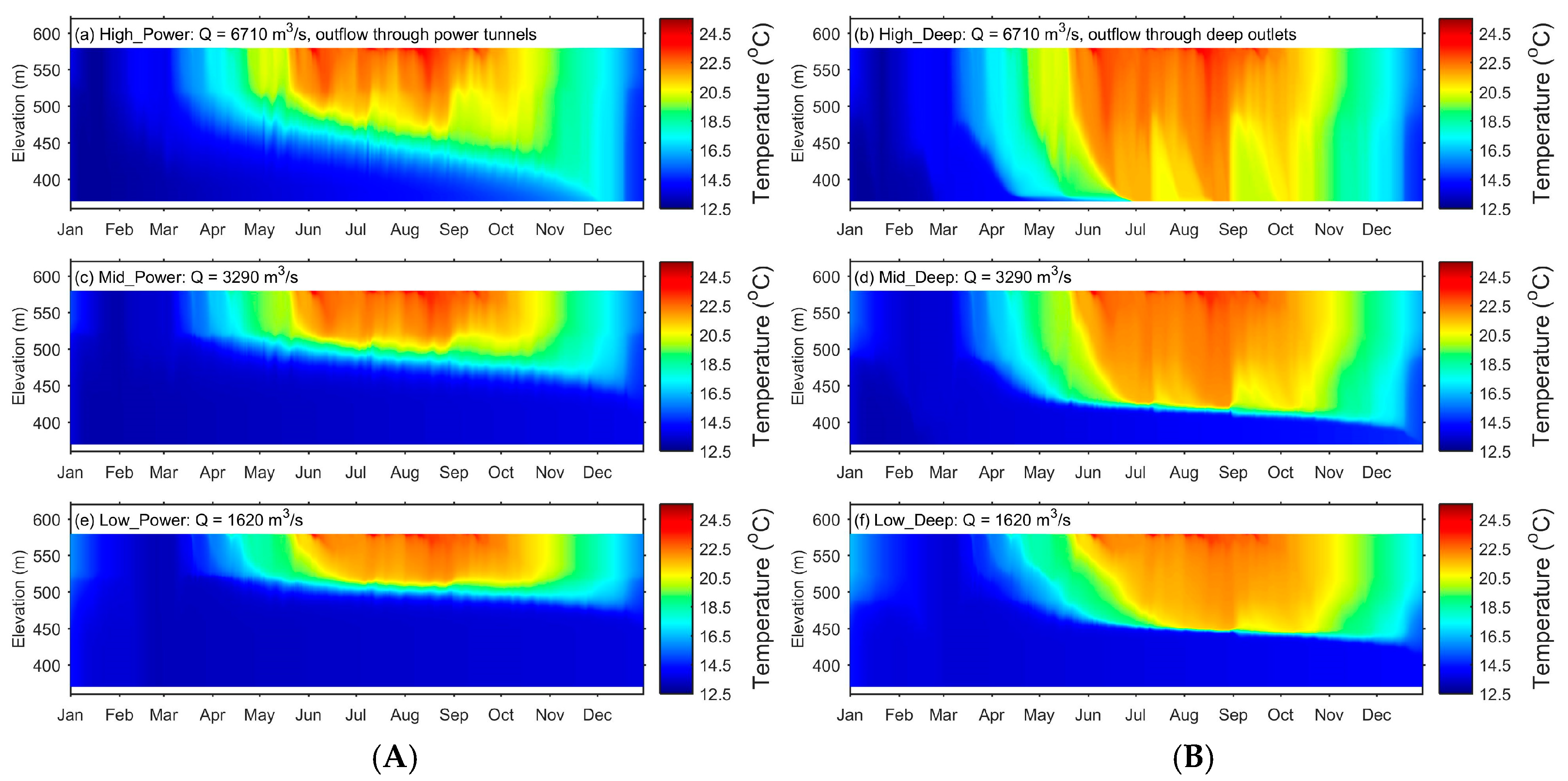
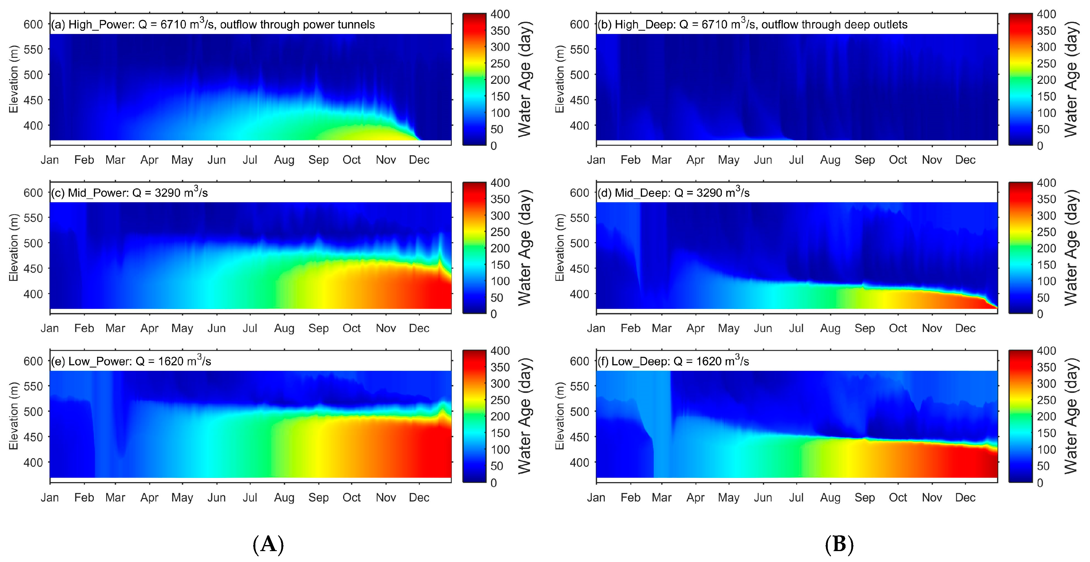
3.4.2. The Influence of Flow Rate

When the inflow and the outflow are low at 1620 m3/s, the hydraulic residence time is ~64 days, the simulated thermal structure at SEG01 is similar to a typical lake having long hydraulic residence time; and during the stratification, the metalimnion deepened slowly if at all (Figure 13e,f). In the High_Power scenario (Table 3), with residence time ~15 days, deepening of the metalimnion is more rapid (Figure 13a) due to the mixing of incoming water with the ambient epilimnetic water. When outflows flow through the power-tunnels (left frames in Figure 13 and Figure 14), as flow rates decreasing from high to low, the elevations of 17 °C isotherm (representing the metalimnion) on 1 July 2014 increase from 453.5, 489.0 to 503.0 m. Between 1 July and 1 October 2014, the average deepening rates of 17 °C isotherm decrease from 0.42, 0.14 to 0.08 m/day, and the average increasing rates of water age at 400 m a.s.l. (in hypolimnion) increase from 0.609, 0.974 to 0.997 days/day (Table 3; Figure 14a,c,e). In the scenarios with the low flow (1620 m3/s), the mixing in the hypolimnion was weak, and the water age increased almost 1 day/day, similar to dead water (Table 3).
The higher inflow not only initiates stratification with a lower metalimnion elevation but also at a higher metalimnetic deepening rate such that a hypolimnion did not form (Figure 13b). As a contrast, in a model study about a subtropical reservoir in Spain where inflow rate was always less than 50 m3/s, a clear relation between initial elevation of the metalimnion and flow rate was found out but it is hard to see any influence of inflow rate on the metalimnion deepening rate in this flow rate range [72].

3.4.3. The Influence of Withdrawn Elevation

The elevation of the metalimnion was heavily affected by the elevation of release structures such as outlets or tunnels [72,77]. In XLDR, the power-tunnels (518 m) are 23 m above the deep outlets (495 m), but the 23-m difference seems to lead to much larger metalimnetic elevation differences at SEG01 in different scenarios (Figure 13). Under the high, middle, and low flow rates (Table 3), the elevations of the metalimnion in scenarios through the deep outlets were 93.5, 68.0, and 51.0 m deeper than those through the power-tunnels, respectively. In the High_Deep scenario (Table 3), the hypolimnion could almost disappear (Figure 13b), and the water age in the whole water column could be low (Figure 14b). The influence of withdrawn elevation may explain the temperature distribution (Figure 8a) and the stronger mixing in 2013 because most of the outflow went through the deep outlets (Figure 2a). In 2014, most of the outflow went through the power tunnels (Figure 2a) before July, and from July to middle of October, the outflow went through both the power tunnels and the deep outlets (Figure 2c), then the deepening of the metalimnion speeded up (Figure 8a).

3.5. The Factors Involving Phase Differences between Inflow and Outflow Temperature

The outflow temperature in a reservoir is generally influenced by a variety of factors such as inflow rates, inflow temperatures, outflow rates, outlet elevations, atmospheric heating, and cooling. Thus it is extremely hard to clearly describe the mechanism behind the phase delay, though the phase delay has been found in many reservoirs [3,5,7,49,71,72,73]. When the inflow to XLDR changed from low in spring, extreme high in summer flood season, to low again in winter (Figure 2), the development of the phase delay was extremely complicated in a real reservoir like XLDR. Due to the variations of the inflow and outflow rate, the daily inflow and outflow temperatures of XLDR in the calibrated scenario fitted with Equation (2) with relatively large RMSE (~1 °C) (Table 4). For the Low_Deep scenario (Table 3), the simulated daily outflow temperatures of XLDR fitted well with Equation (2) with the lowest RMSE (0.33 °C) (Table 4).
The phase shift (−137.4 days) of XLDR’s outflow temperature from the calibration scenario is similar to that (−133.9 days) of the observed outflow temperature in 2014 at XLDG (Figure 4). As the decreasing of flow rate from 6710 to 1620 m3/s, the phase delays increase from 13.20 to 36.78 days in scenarios through the power-tunnels and from 14.70 to 45.47 days through the deep outlets; the latter is slightly larger (Table 4). This indicates the flow rate has strong control on the phase delay in XLDR.
The differences between inflow and outflow temperatures vary seasonally (Figure 15). In spring and early summer, the outflow temperatures are typically lower than the inflow temperatures. In later summer and early fall, the temperatures of the outflow and the inflow are similar. In later fall and winter, the outflow temperatures are slightly larger than the inflow temperatures. During spring and early summer, the inflow is warmed up quickly by the solar heating, but the large thermal inertia from the massive storage (12.3 km3) of XLDR makes the outflow cooler, especially when the inflow is low. During the flood season (July to September 2014), the hydraulic residence time was as low as ~10 days. With the huge amount of water flushing through XLDR as overflow, the inflow goes from the well-mixed condition in the riverine portion through the epilimnion in the stratified portion of XLDR (Figure 8a, or Figure 11c,e), and the inflow temperatures are not much different from the outflow temperatures (Figure 12b). During the winter, the inflow from upstream river cools down faster than the reservoir water, which leads to slightly higher outflow temperatures. The phase delay is relatively small under the large constant inflow because of the dominant overflow and mixing through XLDR.
When ignoring the surface heat flux, the outflow temperature depends on the mixing processes happened from the entrance to the dam in a reservoir. The phase delay can be simplified as a dilution problem, where how much inflow water is used to dilute how much ambient water. The inflow flux determines how much water is used to dilute, and the depth of the epilimnion decides how much water is diluted. The influence of the ambient water volume on dilution could probably explain why, under the same flow rate, the phase delays in scenarios through the deep outlets are higher, for they have deeper epilimnion, which provides more water to be diluted (Figure 15; Table 4).

4. Summary and Conclusions

XLDR is a deep (maximum depth of 240 m) subtropical warm monomictic reservoir. It has both large storage volume (12.3 km3) and high flux (126 km3/year), similar to a running river but quite different from the typical reservoirs or lakes with relatively small flux. We investigated the observed temperatures at four gauge stations (Figure 1) before and after the impoundments of XLDR and XJBR (Figure 3) to find out how the temperature, especially the outflow temperature of XLDR, changed after the impoundments. Then, through simulating water temperatures using a two-dimensional hydrodynamic model, CE-QUAL-W2, we obtained a better understanding of the thermal structure and its variation inside XLDR. Finally, by introducing six hypothetic scenarios into the W2 model, we found out the influences of the dominant factors, flow rates and withdrawn elevations, on the thermal structure of the reservoir and the outflow temperature.
The daily temperature in each year was fitted with Equation (2) (Figure 4), and then the changes of the seasonal temperature were quantified. Before the impoundment, the differences of amplitudes and of the phase delays between PSG (near XJB dam) and HTG were negligible, but the annual average temperature increase from HTG to PSG was not negligible even though it was not large. After the impoundment in May 2013, the annual average and the amplitude of the temperature at HTG, XLDG, and XJBG in 2014 were basically the same as in 2012, but the phase delays between the inflow and outflow of XLDR an XJBR became significantly large (16.5 and 10.6 days). Further analysis of the annual air temperature variations near XLDR (Figure 4c) indicated that the variations of air temperature from 2012 to 2014 were not the reason for the temperature phase delay after the impoundment.
The W2 model was configured to simulate temperatures in XLDR in its first two years of the impoundment using measured data as model input and was calibrated using measured temperature profiles at SEG01 (Figure 6) and outflow temperature at XLDG (Figure 7). The average MAE and RMSE between the 16 measured profiles and the corresponding simulated profiles were 0.30 °C and 0.50 °C, respectively. After analyzing vertical temperature gradients along depth from measured profiles, the threshold of 0.15 °C/m was adapted to identify the upper and lower boundaries of the metalimnion, and the corresponding N was ~10 cph. The calibrated W2 model was applied for simulating temperatures in XLDR under six model scenarios (Table 3) of three constant inflows (inflows = outflows) and discharging through either the power-tunnels (518 m a.s.l.) or the deep outlets (495 m a.s.l.) of the Xiluodu Dam.
In 2013, a short period of stratification in XLDR occurred in June–July (Figure 8a). From 4 December 2013 to 27 January 2014, the colder and denser inflows generated plunging flows (Figure 11a,b) as density currents, and the reservoir was weakly stratified. The net heat flux between inflow and outflow and the surface heat transfer in this period were of the same magnitude. However, the inflow and outflow had the momentum to mix the water mainly from the lower layer, in addition, to remove the heat from the reservoir, but the surface cooling brought about convection from the surface in the upper layer. The vertical temperature was homogeneous in February. From March to August, both the net heat flux of inflow and outflow and the surface heat transfer contributed to the warming up of XLDR, but the net heat flux of inflow and outflow was nearly nine times larger than the surface heat flux. A stable stratification lasted from late April to the end of December 2014 when the warmer and lighter inflow formed overflows passing through the epilimnion, and the stratification vanished at the end of December 2014 after the deepening of the metalimnion reached the reservoir bottom. The calculated water age, vertical temperature gradient, and N at SEG01 depicted the deepening process of the metalimnion (Figure 8), and the average deepening rate was 0.49 m/day. The largest metalimnetic deepening rate due to large inflow (~15,000 m3/s) was 1.67 m/day.
The outflows from XLDR were withdrawn from the epilimnion during the stratification period, and the epilimnetic depth increased from 25 to 215 m in 2014 from May to December, but the thickness of the metalimnion did not change much (19 ± 6.3 m) before the final die-out stage in December (Figure 12). The simulated water ages clearly revealed when and where the underflow, interflow, and overflow occurred in XLDR (Figure 8 and Figure 11). In SEG01, water ages in the epilimnion were about 19.9 ± 8.7 days during the stratification, but the average water ages in the hypolimnion increased linearly from 87.7 to 304.4 days (Figure 12c), with an increase of 0.87 days per day, since the hypolimnetic water stored from the winter or spring density currents was shielded by the metalimnion.
Inflow rate is the dominant factor controlling the deepening speed of the metalimnion. In the scenarios under the low flow (inflow = outflow = 1620 m3/s), the hydraulic residence time is ~64 days. The simulated thermal structure at SEG01 is similar to a typical lake having long hydraulic residence time, and when it is stratified, the metalimnion does not have much deepening (Figure 13e,f). In the scenario under the high flow (6710 m3/s) through the power-tunnels with a hydraulic residence time of ~15 days, deepening of the metalimnion is obviously reflecting inflow momentum, pushing the metalimnion downward continuously (Figure 13a). The deeper outflow withdrawn elevation led to a deeper metalimnion and larger epilimnetic depth (Figure 14).
The phase shift c of XLDR’s outflow temperature from the calibration scenario is −137.4 days which is similar to that (−133.93 days) of the observed temperature at XLDG in 2014 (Figure 4). Those hypothetic scenarios reveal that, under the same outflow withdrawn elevation, the larger inflow rate will produce an outflow with less phase delay, and under the same inflow rate, the phase delays in scenarios through the deep outlets are slightly larger. When the constant inflow/outflow rate is decreased from 6710 to 1620 m3/s (Table 3), the phase delays increase from 13.2 to 36.8 days in three scenarios where the outflows are through the power-tunnels, and the phase delays increase from 14.70 to 45.47 days in scenarios through the deep outlets (Table 4). Previous studies have provided a general description of the phase delay in reservoirs [14], but the phase delay was not quantified, and the phase delays in XLDR under various boundary conditions are still complicated and needed to be quantified and studied further, especially to clearly understand contributing factors and quantify the correlation of phase delay and contributing factors.

Acknowledgments

The authors wish to express their thanks to Xiao Chen, Yang Yu, Kang Yu, Tao Wu, and Xinyu Zuo for helping to collect data. The authors gratefully acknowledge the National Science and Technology Support Project of China (No. 2016YFC0502204) and the financial support from the China Three Gorges Corporation (0799532). Qike Xie wishes to express his gratitude to the Chinese Scholarship Council for the financial support in pursuing his exchange graduate study at the University of California, Santa Barbara.

Author Contributions

Zhaowei Liu and Yongcan Chen conceived and designed the experiments; Qike Xie performed the experiments; Qike Xie, Zhaowei Liu, and Chong Li contributed field sampling and analyzed the data; Qike Xie wrote the paper. Xing Fang worked closely with Qike Xie to revise and improve the paper. Sally MacIntyre provided valuable comments to improve the paper.

Conflicts of Interest

The authors declare no conflict of interest.

References

  1. Owens, E.M.; Effler, S.W.; Trama, F. Variability in thermal stratification in a reservoir. JAWRA J. Am. Water Resour. Assoc. 1986, 22, 219–227. [Google Scholar] [CrossRef]
  2. Shimoda, Y.; Azim, M.E.; Perhar, G.; Ramin, M.; Kenney, M.A.; Sadraddini, S.; Gudimov, A.; Arhonditsis, G.B. Our current understanding of lake ecosystem response to climate change: What have we really learned from the north temperate deep lakes? J. Great Lakes Res. 2011, 37, 173–193. [Google Scholar] [CrossRef]
  3. Webb, B.W.; Walling, D.E. Complex summer water temperature behaviour below a UK regulating reservoir. Regul. Rivers: Res. Manag. 1997, 13, 463–477. [Google Scholar] [CrossRef]
  4. Steel, E.A.; Lange, I.A. Using wavelet analysis to detect changes in water temperature regimes at multiple scales: Effects of multi-purpose dams in the Willamette River basin. River Res. Appl. 2007, 23, 351–359. [Google Scholar] [CrossRef]
  5. Olden, J.D.; Naiman, R.J. Incorporating thermal regimes into environmental flows assessments: Modifying dam operations to restore freshwater ecosystem integrity. Freshw. Biol. 2010, 55, 86–107. [Google Scholar] [CrossRef]
  6. Webb, B.W.; Hannah, D.M.; Moore, R.D.; Brown, L.E.; Nobilis, F. Recent advances in stream and river temperature research. Hydrol. Process. 2008, 22, 902–918. [Google Scholar] [CrossRef]
  7. Caissie, D. The thermal regime of rivers: A review. Freshw. Biol. 2006, 51, 1389–1406. [Google Scholar] [CrossRef]
  8. Webb, B.W.; Nobilis, F. Long term water temperature trends in Austrian rivers. Hydrol. Sci. J. 1995, 40, 83–96. [Google Scholar] [CrossRef]
  9. Webb, B.W.; Walling, D.E. Long-term variability in the thermal impact of river impoundment and regulation. Appl. Geogr. 1996, 16, 211–223. [Google Scholar] [CrossRef]
  10. Hamblin, P.F.; McAdam, S.O. Impoundment effects on the thermal regimes of Kootenay Lake, the Arrow Lakes Reservoir and Upper Columbia River. Hydrobiologia 2003, 504, 3–19. [Google Scholar] [CrossRef]
  11. Rheinheimer, D.E.; Null, S.E.; Lund, J.R. Optimizing selective withdrawal from reservoirs to manage downstream temperatures with climate warming. J. Water Resour. Plan. Manag. 2015, 141. [Google Scholar] [CrossRef]
  12. Chen, G.; Fang, X.; Devkota, J. Understanding flow dynamics and density currents in a river-reservoir system under upstream reservoir releases. Hydrol. Sci. J. 2015. [Google Scholar] [CrossRef]
  13. Lowney, C.L. Stream temperature variation in regulated rivers: Evidence for a spatial pattern in daily minimum and maximum magnitudes. Water Resour. Res. 2000, 36, 2947–2956. [Google Scholar] [CrossRef]
  14. Preece, R.M.; Jones, H.A. The effect of Keepit Dam on the temperature regime of the Namoi River, Australia. River Res. Appl. 2002, 18, 397–414. [Google Scholar] [CrossRef]
  15. Webb, B.W.; Nobilis, F. Long-term changes in river temperature and the influence of climatic and hydrological factors. Hydrol. Sci. J. 2007, 52, 74–85. [Google Scholar] [CrossRef]
  16. Ford, D.E.; Stefan, H. Stratification variability in three morphometrically different lakes under identical meteorological forcing. JAWRA J. Am. Water Resour. Assoc. 1980, 16, 243–247. [Google Scholar] [CrossRef]
  17. Imberger, J. The diurnal mixed layer. Limnol. Oceanogr. 1985, 30, 737–770. [Google Scholar] [CrossRef]
  18. Monismith, S.G.; Imberger, J.; Morison, M.L. Convective motions in the sidearm of a small reservoir. Limnol. Oceanogr. 1990, 35, 1676–1702. [Google Scholar] [CrossRef]
  19. Monismith, S.G. Wind-forced motions in stratified lakes and their effect on mixed-layer shear. Limnol. Oceanogr. 1985, 30, 771–783. [Google Scholar] [CrossRef]
  20. Alcântara, E.H.; Stech, J.L.; Lorenzzetti, J.A.; Bonnet, M.P.; Casamitjana, X.; Assireu, A.T. Remote sensing of water surface temperature and heat flux over a tropical hydroelectric reservoir. Remote Sens. Environ. 2010, 114, 2651–2665. [Google Scholar] [CrossRef]
  21. Riera, J.; Jaume, D.; De Manuel, J.; Morgui, J.; Armengol, J. Patterns of variation in the limnology of Spanish reservoirs: A regional study. Limnetica 1992, 8, 111–123. [Google Scholar]
  22. StrašKraba, M. Limnological basis for modeling reservoir ecosystems. In Man-Made Lakes: Their Problems and Environmental Effects; American Geophysical Union: Washington, DC, USA, 1973; pp. 517–535. [Google Scholar]
  23. Carmack, E.C. Combined influence of inflow and lake temperatures on spring circulation in a riverine lake. J. Phys. Oceanogr. 1979, 9, 422–434. [Google Scholar] [CrossRef]
  24. Nowlin, W.H.; Davies, J.-M.; Nordin, R.N.; Mazumder, A. Effects of water level fluctuation and short-term climate variation on thermal and stratification regimes of a British Columbia reservoir and lake. Lake Reserv. Manag. 2004, 20, 91–109. [Google Scholar] [CrossRef]
  25. Casamitjana, X.; Serra, T.; Colomer, J.; Baserba, C.; Perez-Losada, J. Effects of the water withdrawal in the stratification patterns of a reservoir. Hydrobiologia 2003, 504, 21–28. [Google Scholar] [CrossRef]
  26. Dan, B.M.; Arneson, R.D. Comparative limnology of a deep-discharge reservoir and a surface-discharge lake on the Madison River, Montana. Freshw. Biol. 1978, 8, 33–42. [Google Scholar]
  27. Çalışkan, A.; Elçi, Ş. Effects of selective withdrawal on hydrodynamics of a stratified reservoir. Water Resour. Manag. 2009, 23, 1257–1273. [Google Scholar] [CrossRef]
  28. Chen, G.; Fang, X. Sensitivity analysis of flow and temperature distributions of density currents in a river-reservoir system under upstream releases with different durations. Water 2015, 7, 6244–6268. [Google Scholar] [CrossRef]
  29. Li, Z.; Zhu, D.; Chen, Y.; Fang, X.; Liu, Z.; Ma, W. Simulating and understanding effects of water level fluctuations on thermal regimes in Miyun Reservoir. Hydrol. Sci. J./J. Des Sci. Hydrol. 2016, 61, 952–969. [Google Scholar] [CrossRef]
  30. Akiyama, J.; Stefan, H.G. Gravity Currents in Lakes, Reservoirs and Coastal Regions: Two-Layer Stratified Flow Analysis; St. Anthony Falls Hydraulic Laboratory: Minneapolis, MN, USA, 1987. [Google Scholar]
  31. Akiyama, J.; Stefan, H.G. Plunging flow into a reservoir: Theory. J. Hydraul. Eng. 1984, 110, 484–499. [Google Scholar] [CrossRef]
  32. Alavian, V.; Jirka, G.H.; Denton, R.A.; Johnson, M.C.; Stefan, H.G. Density currents entering lakes and reservoirs. J. Hydraul. Eng.-Asce 1992, 118, 1464–1489. [Google Scholar] [CrossRef]
  33. Alavian, V. Behavior of density currents on an Incline. J. Hydraul. Eng. 1986, 112, 27–42. [Google Scholar] [CrossRef]
  34. Ma, H.; He, H.; Jc, P.; Rs, S. Entrainment into two-dimensional and axisymmetric turbulent gravity currents. J. Fluid Mech. 1996, 308, 289–311. [Google Scholar]
  35. Carmack, E.C.; Gray, C.B.J.; Pharo, C.H.; Daley, R.J. Importance of lake-river interaction on seasonal patterns in the general circulation of Kamloops Lake, British Columbia. Limnol. Oceanogr. 1979, 24, 634–644. [Google Scholar] [CrossRef]
  36. Fischer, H.B.; Smith, R.D. Observations of transport to surface waters from a plunging inflow to Lake Mead. Limnol. Oceanogr. 1983, 28, 258–272. [Google Scholar] [CrossRef]
  37. Alavian, V.; Ostrowski, P. Use of density current to modify thermal structure of TVA reservoirs. J. Hydraul. Eng. 1992, 118, 688–706. [Google Scholar] [CrossRef]
  38. Dallimore, C.J.; Imberger, J.R.; Ishikawa, T. Entrainment and turbulence in saline underflow in Lake Ogawara. J. Hydraul. Eng. 2001, 127, 937–948. [Google Scholar] [CrossRef]
  39. Benyahya, L.; Sthilaire, A.; Quarda, T.B.M.J.; Bobée, B.; Ahmadinedushan, B. Modeling of water temperatures based on stochastic approaches: Case study of the Deschutes River. J. Environ. Eng. Sci. 2007, 6, 437–448. [Google Scholar] [CrossRef]
  40. Cole, T.M.; Wells, S.A. CE-QUAL-W2: A Two-Dimensional, Laterally Averaged, Hydrodynamic and Water Quality Model; Version 3.71; User Manual; Department of Civil and Environmental Engineering, Portland State University: Portland, OR, USA, 2013. [Google Scholar]
  41. Hanna, R.B.; Saito, L.; Bartholow, J.M.; Sandelin, J. Results of simulated temperature control device operations on in-reservoir and discharge water temperatures using CE-QUAL-W2. Lake Reserv. Manag. 1999, 15, 87–102. [Google Scholar] [CrossRef]
  42. Kurup, R.G.; Hamilton, D.P.; Phillips, R.L. Comparison of two 2-dimensional, laterally averaged hydrodynamic model applications to the Swan River Estuary. In Mathematics and Computers in Simulation; Elsevier Science Publishers B. V.: Amsterdam, The Netherlands, 2000; Volume 51, pp. 627–638. [Google Scholar]
  43. Debele, B.; Srinivasan, R.; Parlange, J.Y. Coupling upland watershed and downstream waterbody hydrodynamic and water quality models (SWAT and CE-QUAL-W2) for better water resources management in complex river basins. Environ. Model. Assess. 2008, 13, 135–153. [Google Scholar] [CrossRef]
  44. Kim, Y.; Kim, B. Application of a 2-dimensional water quality model (CE-QUAL-W2) to the turbidity interflow in a deep reservoir (Lake Soyang, Korea). Lake Reserv. Manag. 2009, 22, 213–222. [Google Scholar] [CrossRef]
  45. Mooij, W.M.; Trolle, D.; Jeppesen, E.; Arhonditsis, G.; Belolipetsky, P.V.; Chitamwebwa, D.B.R.; Degermendzhy, A.G.; DeAngelis, D.L.; De Senerpont Domis, L.N.; Downing, A.S.; et al. Challenges and opportunities for integrating lake ecosystem modelling approaches. Aquat. Ecol. 2010, 44, 633–667. [Google Scholar] [CrossRef] [Green Version]
  46. Deliman, P.N.; Gerald, J.A. Application of the two-dimensional hydrothermal and water quality model, CE-QUAL-W2, to the Chesapeake Bay–Conowingo Reservoir. Lake Reserv. Manag. 2002, 18, 10–19. [Google Scholar] [CrossRef]
  47. Bowen, J.D.; Hieronymus, J.W. A CE-QUAL-W2 model of Neuse Estuary for total maximum daily load development. J. Water Resour. Plan. Manag. 2003, 129, 283–294. [Google Scholar] [CrossRef]
  48. Rangel-Peraza, J.; Obregon, O.; Nelson, J.; Williams, G.; De Anda, J.; González-Farías, F.; Miller, J. Modelling approach for characterizing thermal stratification and assessing water quality for a large tropical reservoir. Lakes Reserv.: Res. Manag. 2012, 17, 119–129. [Google Scholar] [CrossRef]
  49. Dai, L.; Dai, H.; Jiang, D. Temporal and spatial variation of thermal structure in Three Gorges Reservoir: A simulation approach. J. Food Agric. Environ. 2012, 10, 1174–1178. [Google Scholar]
  50. Gang, C.; Xing, F. Accuracy of hourly water temperatures in rivers calculated from air temperatures. Water 2015, 7, 1068–1087. [Google Scholar]
  51. Tim Kraft, P.E. Green River CE-QUAL-W2 Project: A Hydrodynamic and Water Quality Study of the Green River King County, Washington; King County Department of Natural Resources and Parks: Seattle, WA, USA, 2004; pp. 1–280.
  52. Ostfeld, A.; Salomons, S. A hybrid genetic—Instance based learning algorithm for CE-QUAL-W2 calibration. J. Hydrol. 2005, 310, 122–142. [Google Scholar] [CrossRef]
  53. Zhang, H.; Culver, D.A.; Boegman, L. A two-dimensional ecological model of Lake Erie: Application to estimate dreissenid impacts on large lake plankton populations. Ecol. Model. 2008, 214, 219–241. [Google Scholar] [CrossRef]
  54. Blandford, T.R.; Humes, K.S.; Harshburger, B.J.; Moore, B.C.; Walden, V.P.; Ye, H. Seasonal and synoptic variations in near-surface air temperature lapse rates in a mountainous basin. J. Appl. Meteorol. Climatol. 2008, 47, 9–10. [Google Scholar] [CrossRef]
  55. Gardner, A.S.; Sharp, M.J.; Labine, C.; Boon, S.; Burgess, D.O.; Lewis, D.; Koerner, R.M.; Marshall, S.J. Near-surface temperature lapse rates over Arctic glaciers and their implications for temperature downscaling. J. Clim. 2009, 22, 4281–4298. [Google Scholar] [CrossRef]
  56. Minder, J.R.; Mote, P.W.; Lundquist, J.D. Surface temperature lapse rates over complex terrain: Lessons from the Cascade Mountains. J. Geophys. Res. 2010, 115, 1307–1314. [Google Scholar] [CrossRef]
  57. Gouvas, M.A.; Sakellariou, N.K.; Kambezidis, H.D. Estimation of the monthly and annual mean maximum and mean minimum air temperature values in Greece. Meteorol. Atmos. Phys. 2011, 110, 143–149. [Google Scholar] [CrossRef]
  58. Kattel, D.B.; Yao, T.; Yang, K.; Tian, L.; Yang, G.; Joswiak, D. Temperature lapse rate in complex mountain terrain on the southern slope of the central Himalayas. Theor. Appl. Climatol. 2013, 113, 671–682. [Google Scholar] [CrossRef]
  59. Buck, A.L. New Equations for Computing Vapor Pressure and Enhancement Factor. J. Appl. Meteorol. 1981, 20, 1527–1532. [Google Scholar] [CrossRef]
  60. Buck, A.L. Buck Research CR-1A User’s Manual; Buck Research Instruments: Boulder, CO, USA, 1996. [Google Scholar]
  61. Ahmadi-Nedushan, B.; St-Hilaire, A.; Ouarda, T.B.M.J.; Bilodeau, L.; Robichaud, É.; Thiémonge, N.; Bobée, B. Predicting river water temperatures using stochastic models: Case study of the Moisie River (Québec, Canada). Hydrol. Process. 2007, 21, 21–34. [Google Scholar] [CrossRef]
  62. Caissie, D.; Eljabi, N.; Sthilaire, A. Stochastic modelling of water temperatures in a small stream using air to water relations. Can. J. Civ. Eng. 2011, 25, 250–260. [Google Scholar] [CrossRef]
  63. Chen, G.; Fang, X.; Fan, H. Estimating hourly water temperatures in rivers using modified sine and sinusoidal wave functions. J. Hydrol. Eng. 2016, 21. [Google Scholar] [CrossRef]
  64. Webb, B.W.; Walling, D.E. Longer-term water temperature behaviour in an upland stream. Hydrol. Process. 1993, 7, 19–32. [Google Scholar] [CrossRef]
  65. Cluis, D.A. Relationship between stream water temperature and ambient air temperature—A simple autoregressive model for mean daily stream water temperature fluctuations. Hydrol. Res. 1972, 3, 65–71. [Google Scholar]
  66. Rueda, F.; Moreno-Ostos, E.; Armengol, J. The residence time of river water in reservoirs. Ecol. Model. 2006, 191, 260–274. [Google Scholar] [CrossRef]
  67. Gong, W.; Shen, J.; Hong, B. The influence of wind on the water age in the tidal Rappahannock River. Mar. Environ. Res. 2009, 68, 203–216. [Google Scholar] [CrossRef] [PubMed]
  68. Zhang, W.G.; Wilkin, J.L.; Schofield, O.M.E. Simulation of water age and residence time in New York Bight. J. Phys. Oceanogr. 2010, 40, 965–982. [Google Scholar] [CrossRef]
  69. Li, Y.; Acharya, K.; Yu, Z. Modeling impacts of Yangtze River water transfer on water ages in Lake Taihu, China. Ecol. Eng. 2011, 37, 325–334. [Google Scholar] [CrossRef]
  70. Imberger, J.; Hamblin, P.F. Dynamics of lakes, reservoirs, and cooling ponds. Annu. Rev. Fluid Mech. 1982, 14, 153–187. [Google Scholar] [CrossRef]
  71. Pozo, J.; Orive, E.; Fraile, H.; Basaguren, A. Effects of the Cernadilla–Valparaiso reservoir system on the River Tera. Regul. Rivers: Res. Manag. 1997, 13, 57–73. [Google Scholar] [CrossRef]
  72. Han, B.-P.; Armengol, J.; Garcia, J.C.; Comerma, M.; Roura, M.; Dolz, J.; Straskraba, M. The thermal structure of Sau Reservoir (NE: Spain): A simulation approach. Ecol. Model. 2000, 125, 109–122. [Google Scholar] [CrossRef]
  73. Yang, M.; Li, L.; Li, J. Prediction of water temperature in stratified reservoir and effects on downstream irrigation area: A case study of Xiahushan reservoir. Phys. Chem. Earth Parts A/B/C 2012, 53, 38–42. [Google Scholar] [CrossRef]
  74. McQuivey, R.S.; Keefer, T.N. Simple method for predicting dispersion in streams. J. Environ. Eng. Div. 1974, 100, 997–1011. [Google Scholar]
  75. Rueda, F.J.; MacIntyre, S. Flow paths and spatial heterogeneity of stream inflows in a small multibasin lake. Limnol. Oceanogr. 2009, 54, 2041–2057. [Google Scholar] [CrossRef]
  76. Fischer, H.B.; List, J.E.; Koh, C.R.; Imberger, J.; Brooks, N.H. Mixing in Inland and Coastal Waters; Elsevier: Amsterdam, The Netherlands, 1979. [Google Scholar]
  77. Wang, S.; Qian, X.; Han, B.-P.; Wang, Q.-H.; Ding, Z.-F. Physical limnology of a typical subtropical reservoir in south China. Lake Reserv. Manag. 2011, 27, 149–161. [Google Scholar] [CrossRef]
Figure 1. The impoundment areas and surrounding topography of the Xiluodu Reservoir (XLDR) and the Xiangjiaba Reservoir (XJBR); the locations of nearby weather stations, gauge stations, and dams are marked; the elevation (above sea level) of weather stations are labeled. The Baihetan Reservoir is still under construction. The descriptions of these sites are summarized in Table 1.
Water 09 00603 g001
Figure 2. (a) Measured outflow of Xiluodu Reservoir (XLDR) (total outflow and outflows through power-tunnels, flood-tunnels and deep outlets) and the maxima, minima, 75th, 65th, and 15th percentile outflows from accumulative curve of 2014; (b) Measured water surface elevation, computed inflow at the entrance cross-section of XLDR (ENCS) and measured inflow at Huatan gauge station (HTG) from May 2013 to December 2014; (c) Hydraulic residence time of XLDR with annual averages and averages plus/minus standard deviations from May 2013 to December 2013 and from January 2014 to December 2014 separately.
Water 09 00603 g002
Figure 3. (a) Daily water temperatures measured at Huatan gauge station (HTG) and Pinshan gauge station (PSG) from 2000 to 2011, and calculated temperature difference (PSG minus HTG). Average temperature difference was 1.21 ± 0.66 °C; (b) Daily water temperatures measured at HTG, the entrance cross-section of Xiluodu Reservoir (ENCS), Xiluodu gauge station (XLDG), and Xiangjiaba gauge station (XJBG) from 1 January 2012 to 31 December 2014; the light blue line represents temperature differences between XJBG and XLDG, and the red dashed lines represent the average differences from January to June.
Water 09 00603 g003
Figure 4. (ac) The coefficients a, b, and c of the annual variations determined by fitting daily temperatures using Equation (2) and the least-square-error method at Huatan gauge station (HTG) (2000–2014), Pinshan gauge station (PSG) (2000–2011), Xiangjiaba gauge station (XJBG) (2012–2014) and Xiluodu gauge station (XLDG) (2012, 2014); (d) Root mean square error (RMSE) of the fitted curve in each year. The dash lines marked the impoundment dates of Xiangjiaba Reservoir (XJBR) and Xiluodu Reservoir (XLDR).
Water 09 00603 g004
Figure 5. Simulated temperature profiles at a cross-section 3.5 km upstream to the Xiluodu Dam (SEG01) using four Ax (Dx = Ax) and observed profiles on 9 September 2014 (a); 13 August 2014 (b); and 15 October 2014 (c).
Water 09 00603 g005
Figure 6. Simulated and observed vertical temperature profiles at a cross-section 3.5 km upstream to the Xiluodu Dam (SEG01) (bottom x axis) and vertical temperature gradient (top x axis) calculated using observed vertical temperatures.
Water 09 00603 g006
Figure 7. Simulated and observed outflow temperatures from Xiluodu Reservoir (XLDR) in 2014 Xiluodu gauge station (XLDG) is at 2.9 km downstream of the Xiluodu Dam).
Water 09 00603 g007
Figure 8. Contour plots of (a) water temperature; (b) water age; (c) vertical temperature gradient; and (d) buoyancy frequency (N) at a cross-section 3.5 km upstream to the Xiluodu Dam (SEG01) from 4 May 2013 to 31 December 2014. During the stratification of 2014, the Xiluodu Reservoir (XLDR) outflow was mainly drawn from the epilimnion by the power-tunnels (entrance elevation was 518–528 m a.s.l.), and the deep outlets (entrance elevation was 495–505 m a.s.l.) were used to release a part of the flood peak (Figure 2a).
Water 09 00603 g008
Figure 9. The vertical temperature gradient and N calculated from observed temperature profiles on 14 April (a), 9 June (b), 19 July (c), and 15 October (d) of 2014. The red line is the temperature gradient, the blue line is N, and the black line is the temperature.
Water 09 00603 g009
Figure 10. Simulated daily total heat flux through the reservoir surface (positive for the reservoir to absorb heat, the second y axis) including long and short wave radiation, convective heat flux and evaporative flux; the daily equivalent net heat flux of flow (inflow minus outflow, the first y axis), calculated based on Equations (7) and (8).
Water 09 00603 g010
Figure 11. Longitudinal profiles of simulated temperature (left panels; a, c, and e) and water age (right panels; b, d, and f) from the entrance cross-section of Xiluodu Reservoir (ENCS) to the dam of Xiluodu Reservoir (XLDR) on 2 January (top; a and b), 1 June (middle; c and d) and 1 August (bottom; e and f) 2014. The inflow was ~2000 m3/s on 2 January and 1 June and ~8000 m3/s on 1 August. The plunging point was about 45 km downstream ENCS on 2 January 2014 when inflow was low (2000 m3/s) and inflow temperature was 13.0 °C. The warmer and lighter inflow traveled through the epilimnion from ENCS to a cross-section 3.5 km upstream to the Xiluodu Dam (SEG01) and formed an overflow on 1 June and 1 August 2014.
Water 09 00603 g011
Figure 12. (a) Average layer elevation with upper and lower boundaries for epilimnion (green), metalimnion (red) and hypolimnion (blue) of a cross-section 3.5 km upstream to the Xiluodu Dam (SEG01) in stable stratification period of 2014 from CE-QUAL-W2 (W2) model; (b) Mass weighted layer-averaged temperatures for epilimnion (green), metalimnion (red) and hypolimnion (blue) of SEG01, inflow and outflow temperature during seasonal stratification period of 2014 from W2 model; (c) Average water ages of each layer. The upper and lower boundaries of the metalimnion were identified by a temperature gradient of 0.15 °C/m.
Water 09 00603 g012
Figure 13. Simulated water temperature at a cross-section 3.5 km upstream to the Xiluodu Dam (SEG01) under six scenarios. (A): outflows are through power-tunnels. (B): through deep outlets. Flow rates decrease from upper to lower panels. Deep outlets were at 495 m a.s.l. and power-tunnels were at 518 m a.s.l. Comparing results from left and right reveals the impact from outflow through either the power-tunnels or the deep outlets; results from upper and lower panels indicate the impact from high to low flow rates. For all three flow rates, when the outflows were through the deep outlets, the epilimnion and metalimnion are deeper, or the hypolimnion is thinner, in comparison to the outflows through the power-tunnels.
Water 09 00603 g013
Figure 14. Simulated water age at a cross-section 3.5 km upstream to the Xiluodu Dam (SEG01) under three inflow scenarios. (A): outflows are through power-tunnels. (B): through deep outlets. Flow rates decrease from upper to lower panels. At all situations, outflows were withdrawn from the epilimnion with smaller water age. Other details were as in Figure 13.
Water 09 00603 g014
Figure 15. The simulated outflow temperatures of the six scenarios in Table 3 and of the calibration scenario, as well as the inflow temperature at the entrance cross-section of Xiluodu Reservoir (ENCS), from 4 May 2013 to 31 December 2014. Cali. refers to the calibration scenario of the CE-QUAL-W2 (W2) model, which represents the real condition of Xiluodu Reservoir (XLDR). D and P on the legends refer to the outflows through the deep outlets and the power-tunnels, respectively.
Water 09 00603 g015
Table 1. Abbreviations and their descriptions used in this study.
AbbreviationDescription
XLDRXiluodu Reservoir (Impoundment since 2013)
XJBRXiangjiaba Reservoir (Impoundment since 2012)
BHTRBaihetan Reservoir (Estimated impoundment in 2022)
HTGHuatan gauge station (235.1 km upstream to the Xiluodu Dam)
XLDGXiluodu gauge station (2.9 km downstream to the Xiluodu Dam)
PSGPinshan gauge station (29.1 km upstream to the Xiangjiaba Dam)
XJBGXiangjiaba gauge station (2.4 km downstream to the Xiangjiaba Dam)
JYJinyang weather station
SEG01A cross-section 3.5 km upstream to the Xiluodu Dam
ENCSThe entrance cross-section of XLDR (155 km upstream to the Xiluodu Dam)
W2CE-QUAL-W2
Table 2. Monthly average air temperature lapse rate ( k , air temperature increase rate per 100 m downwards) and corresponding R2 (goodness of the linear regressions) in the Xiluodu Reservoir (XLDR) region determined by linear regressions of monthly air temperatures in 11 weather stations at different elevations (Figure 1) from 2000 to 2014.
MonthJanuaryFebruaryMarchAprilMayJuneJulyAugustSeptemberOctoberNovemberDecember
k (°C/100 m)0.3560.3000.3510.3850.4200.4290.4520.4640.4170.4130.4060.385
R20.8930.8180.8770.9150.9550.9850.9910.9920.9840.9780.9620.927
Table 3. Model scenarios which are the combinations of three inflow rates (equal to outflow rates; high, middle, and low in Figure 2a) and two outflows modes (all outflow through the power tunnels or the deep outlets); simulated average deepening rate of 17 °C isotherm and water age increasing rate at 400 m from 1 July 2014 to 1 October 2014 at a cross-section 3.5 km upstream to the Xiluodu Dam (SEG01).
ScenariosHigh_PowerHigh_DeepMid_PowerMid_DeepLow_PowerLow_Deep
Outflow ThroughPower tunnelsDeep outletsPower tunnelsDeep outletsPower tunnelsDeep outlets
Percentile of outflow75%75%65%65%15%15%
Constant flow Rate (m3/s)671067103290329016201620
17 °C isotherm‘s elevation (m a.s.l.) (in metalimnion)1 July 2014453.5Bottom489.0421.0503.5452.5
1 October 2014415.0Bottom476.0410.0496.0442.0
Deep. Rate (m/day)0.42/0.140.120.080.11
Water Age (day) at 400 m a.s.l. (in hypolimnion)1 July 201414911.0184.3170.0187.9202.7
1 October 201420513.6273.9260.0279.6293.8
Incre. Rate (days/day)0.6090.0280.9740.9780.9970.990
Table 4. The coefficients a, b, c, and root mean square error (RMSE) (using Equation (2) and the least-square-error method) of the daily outflow temperatures of the six model scenarios and of the calibration scenario, as well as the model inflow temperature in 2014. The phase delay is calculated by c of the outflow in each scenario minus c of the inflow at the entrance cross-section of Xiluodu Reservoir (ENCS).
ScenarioTypea (°C)b (°C)c (Days)Phase Delay (Days)RMSE (°C)
CalibrationENCS Inflow18.784.01−110.23 0.96
Outflow18.184.29−137.4427.201.00
High_DeepOutflow18.514.32−124.9414.700.83
Mid_DeepOutflow18.224.37−137.0426.810.64
Low_DeepOutflow17.684.23−155.7145.470.33
High_PowerOutflow18.514.26−123.4313.200.88
Mid_PowerOutflow18.274.31−131.9821.750.73
Low_PowerOutflow17.884.27−147.0236.780.46

