Two Dimension Reduction Methods for Multi-Dimensional Dynamic Programming and Its Application in Cascade Reservoirs Operation Optimization

Abstract

An efficient reservoir operation technique plays a very important role in improving the water resources and energy efficiency of reservoirs. In order to effectively avoid or alleviate the “curse of dimensionality” of Multi-dimensional Dynamic Programming (MDP) in the application of cascade reservoirs operation optimization (CROO) and keep a global convergence at the same time, two dimension reduction methods are proposed in this paper. One is a hybrid algorithm of MDP and a Progressive Optimality Algorithm (POA), named MDP-POA, which combines the global convergence of MDP and the strong local search ability of POA. MDP-POA first takes the global optimal trajectory of MDP in a low discrete degree as the initial trajectory of the POA, and then implements further optimization to the obtained initial trajectory by the POA with a high discrete degree, so as to avoid the “curse of dimensionality” of MDP in high discrete degree and the dependency of the POA for the initial trajectory. The other is an improved MDP (IMDP), which first constructs a corridor by the optimal trajectory of MDP in a lower discrete degree, and then implements further optimization in the corridor by MDP with a relatively high discrete degree, so as to avoid a large number of unnecessary calculations, and shorten the run-time effectively. In a case study, the results of MDP-POA, IMDP, and MDP are compared and analyzed from the aspects of power generation and run-time. The analysis indicates that the proposed MDP-POA and IMDP both have a good application effect and are worthy of further promotion.

1. Introduction

As one of the most stable forms of renewable energy, hydropower energy can be commercially developed and utilized on a large scale [1,2,3,4]. With the rapid development of cascade reservoirs, cascade reservoirs operation optimization (CROO) is attracting the attention of more and more scholars all over the world [5,6]. The global optimal solution of CROO has very important practical significance in developing long-term optimal operation schemes and rules for cascade reservoirs [7,8]. So, it is very necessary to solve the CROO problem correctly and reasonably. However, CROO is a multivariate coupled and complicated nonlinear programming problem [9], which needs to consider not only the hydraulic connection between upstream and downstream reservoirs, but also a lot of constraints. It has the characteristics of high dimensionality, strong coupling, and uncertainty [10,11,12], and its solution is full of difficulties and has always been the focus of many scholars’ research [13].

Aiming at the solving of the CROO problem, a wide range of methods have been proposed over the past decades, which mainly involve conventional optimization algorithms and various heuristic random search algorithms [14,15]. The conventional methods include Linear Programming (LP) [16], Nonlinear Programming (NLP) [17], Lagrangian Relaxation (LR) [18], Quadratic Programming (QP) [19], and Multi-dimensional Dynamic Programming (MDP) [20,21]. They are all elitist algorithms, and have already received different degrees of success in solving CROO problems. The modern heuristic random search algorithms include the Genetic Algorithm (GA) [22], Particle Swarm Optimization (PSO) [23], Ant Colony Optimization (ACO) [24], Fuzzy Neural Network (FNN) [25], and the Differential Evolution algorithm (DE) [26,27,28]. These have been extensively used to solve the CROO problem, and have also received a good application effect.

Among the above algorithms, MDP is a powerful optimization technique for CROO problems. The most significant characteristic of MDP is that it is able to obtain a global optimal solution and have no requirement for the initial trajectories. Moreover, MDP imposes no restrictions on the unsmooth and nonconvex nature of CROO problems, which make it boast high popularity among the conventional optimization techniques. Many evolutionary algorithms have been proved to possess a global convergence, while as these algorithms are affected by a stochastic feature, they cannot guarantee a global optimum with finite iterations [29]. However, although the MDP can solve CROO problems with a global convergence, the high dimensionality, called the “curse of dimensionality”, poses difficulties and limits its application in CROO problems, especially for large-scale hydropower systems [30].

On the whole, there are three ways to avoid or alleviate the “curse of dimensionality” and guarantee the global convergence of MDP. The first one is to improve MDP effectively on the premise of guaranteeing a global convergence, so as to shorten the run-time. The second one is to implement parallel computing by using multi-core processing technology. The third one is to combine MDP with other algorithms which have a high computational efficiency, so as to make up for their deficiencies of each other. Some scholars have done related research work in these aspects, as described below.

In terms of algorithm improvements, a variety of improved Dynamic Programming (DP) algorithms have emerged and been used to avoid or alleviate the “curse of dimensionality”, such as the Progressive Optimality Algorithm (POA) [31], Dynamic Programming with Successive Approximation (DPSA) [32], Discrete Differential Dynamic Programming (DDDP) [33], and Incremental Dynamic Programming (IDP) [34]. These improved algorithms can effectively avoid the “curse of dimensionality” to a certain degree, but defects still exist. For example, POA is sensitive to the initial trajectories, and may converge to a local optimum in some situations. DPSA and DDDP are difficult to use to solve problems with non-convexity, and may also lead to a local optimum. In addition, other related research has been done by some scholars. For example, Mousavi et al. [35] reduced the run-time of an MDP model for a multi-reservoir system by diagnosing infeasible storage combinations and removing them from further computations, which has a good effect within a certain amount of hydropower stations, but the time consumption is still enormous and intolerable when the scale of a hydropower system reaches a certain large degree. By taking advantage of the monotonic relationship between reservoir storage volume and the optimal release decision. Zhao et al. [36] proposed an improved DP model for reservoir operation optimization (ROO); however, the model can only be applied to a reservoir operation with a concave objective function. Ji et al. [37] proposed a novel multi-layer nested multi-dimensional dynamic programming (MNDP) based on a multi-layer nested structure, but it was mainly used to deal with the problem of computer memory space and computational complexity for MDP in CROO, and the computing time had not been reduced.

In recent years, parallel computing has been widely applied in the field of water resources [38,39]. Especially, in the field of CROO and MDP applications, there are several successful examples. Dias et al. [40] improved the performance of stochastic dynamic programming by using parallel processing techniques, and successfully applied it to the long-term operation planning of an electrical power system. Li et al. [41] developed a parallel MDP algorithm to optimize the joint operation of a multi-reservoir system based on a distributed memory architecture and the Message Passing Interface (MPI) protocol. Ji et al. [37] implemented parallel computing to the proposed MNDP algorithm, and achieved a good application effect. In order to evaluate the parallel performance of different parallel modes, Zhang et al. [11] proposed three kinds of parallel MDP algorithms. On the whole, these previous studies demonstrate that run-time can be reduced a lot in optimization or simulation by using parallel computing associated with proper parallelization strategies. However, with the increase of the number of cores used in parallel computing, the parallel efficiency will reduce gradually; specifically, when the number of cores is large, the parallel efficiency is generally very low.

In terms of hybrid applications, i.e., the combination usage of MDP with other algorithms, much related research has been achieved, for example, a combination of the GA and DDDP approaches (GA-DDDP) was proposed and developed to optimize a multiple reservoir system’s operation by Tospornsampan et al. [42], and the significant advantage obtained from using GA-DDDP is economizing on computational resources, as GA-DDDP does not require optimizing parameters and the derivation of feasible initial trial trajectories. Lantoine and Russell [43] presented a hybrid variant of the differential dynamic programming (HDDP) algorithm to solve constrained nonlinear optimal control problems, and the hybrid method incorporates nonlinear mathematical programming techniques to increase its efficiency. Zhang et al. [23] joined parallel deterministic dynamic programming and a hierarchical adaptive genetic algorithm to solve an ROO problem. However, in view of the above description and analysis, the effective existing hybrid applications have mainly focused on improved dynamic programming algorithms (such as DDDP and IDP) or intelligent optimization algorithms, and there are very few hybrid applications about the baseline MDP which can converge to the optimal solution without an additional requirement of unsmooth, non-convexity, and initial trajectories. Therefore, it has an important practical significance to carry out research of dimension reduction methods for MDP.

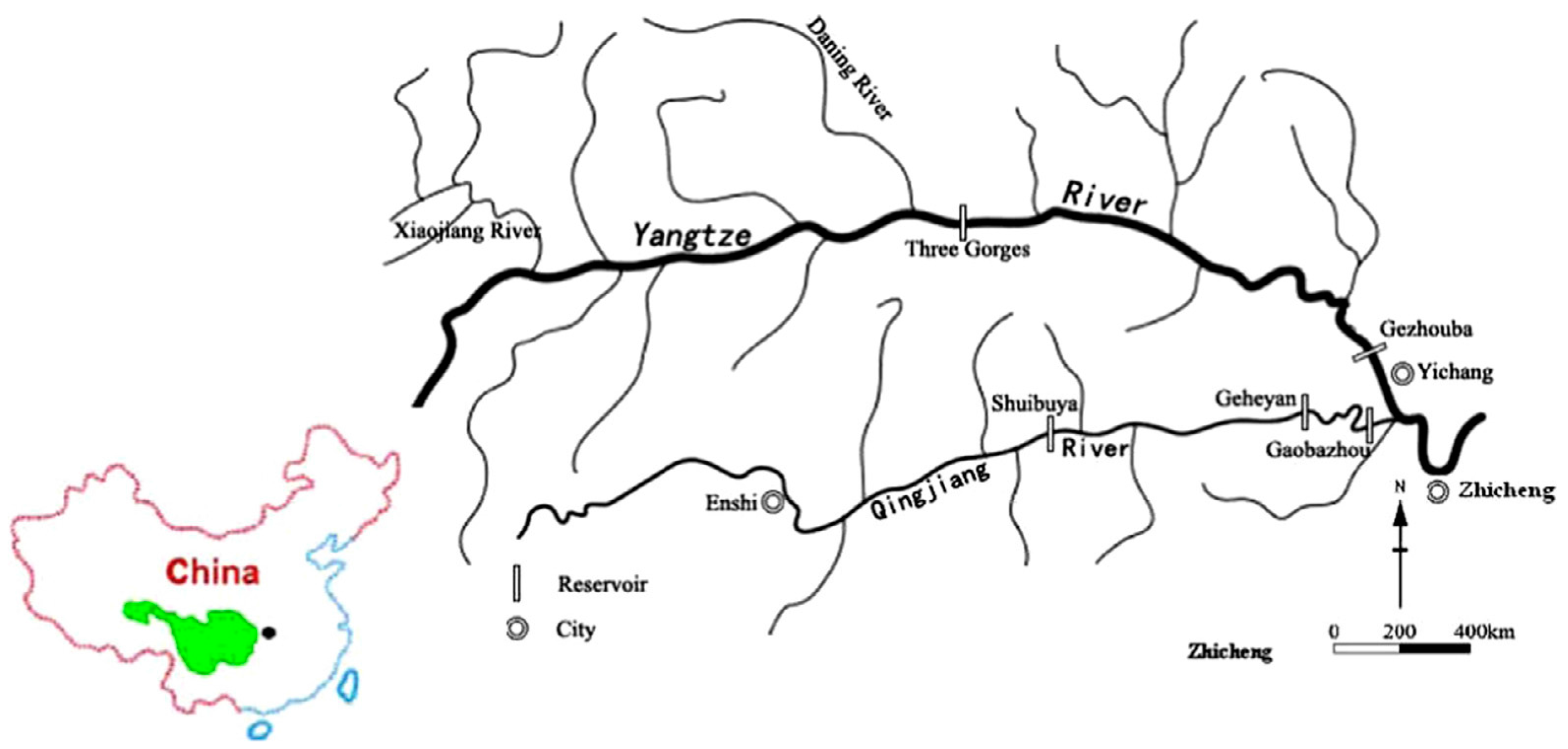
In order to effectively avoid the “curse of dimensionality” of MDP and guarantee a global convergence at the same time, this paper proposes two new dimension reduction methods for MDP based on a structural and characteristics analysis, i.e., a hybrid algorithm of MDP and POA (named MDP-POA), and an improved MDP (named IMDP). A detailed case study was provided in this paper by taking the Qingjiang cascade reservoirs in China as an instance, and in order to evaluate the performance of the proposed MDP-POA and IMDP, the results of MDP-POA, IMDP, and MDP were compared and analyzed from the aspects of power generation and run-time. In addition, the authors have analyzed the varying characteristics of the optimal solution for the proposed MDP-POA and IMDP under different discretization levels, and provided the recommended discretization levels or computing schemes for different conditions. The following part of this paper is organized as follows. Section 2 presents the formulation of CROO problems. Section 3 introduces the principle of MDP and the POA, and presents the optimization principle of MDP-POA and IMDP. Section 4 shows the application of MDP-POA and IMDP in the cascade reservoirs of Qingjiang River in China, and the results are analyzed and discussed in this section. Section 5 presents the conclusions.

2. Formulation of CROO Problems

Power generation is a significant benefit derived from a cascade reservoirs system. CROO aims at maximizing the power generation by developing an optimal plan over the entire planning horizon, while satisfying all kinds of physical and operational constraints. Generally, CROO is related to a given operation of the hydropower stations for T stages as follows.

$$E=\max {\displaystyle \sum _{i=1}^n{\displaystyle \sum _{t=1}^T{{\displaystyle N}}_t^i}\cdot \mathsf{\Delta }t}$$

(1)

$${{\displaystyle N}}_t^i={{\displaystyle K}}_{}^i\cdot {{\displaystyle q}}_t^i\cdot {{\displaystyle H}}_t^i$$

(2)

where E is the total power generation over the entire planning horizon, unit: kWh; T is the number of stages over the entire planning horizon; ${{\displaystyle N}}_t^i$ is the output of the ith hydropower station in the tth stage, unit: kW, and the reservoir indexes from upstream to downstream are 1, 2, ... , n in this paper; Kⁱ is the efficiency coefficient of the ith hydropower station; ${{\displaystyle H}}_t^i$ is the average water level of the ith hydropower station in the tth stage, unit: m, and it is determined by the beginning water level h_t of the tth stage of the reservoir, the end water level h_t+1, and the downstream tail water level h_down, i.e., H_t = (h_t + h_t+1)/2 − h_down, while h_down is determined by the total outflow Q_t of the reservoir in the tth stage, and Q_t happens to be determined by h_t and h_t+1. In addition, the reservoir water level h has a one-to-one mapping relationship with the reservoir volume V, namely the reservoir curve of water level–volume; Δt is the duration of a stage, unit: h. CROO is subject to the following equality and inequality constraints.

(1) Water volume balance:

$${{\displaystyle q}}_t^i=\left({{\displaystyle V}}_{t-1}^i-{{\displaystyle V}}_t^i\right)/3600\Delta t+{{\displaystyle I}}_t^i+{{\displaystyle Q}}_t^{i-1}-{{\displaystyle W}}_t^i-{{\displaystyle Ev}}_t^i$$

(3)

where ${{\displaystyle q}}_t^i$ is the outflow through the turbines of the ith reservoir in the tth stage, unit: m³/s; ${{\displaystyle W}}_t^i$ is the abandoned water outflow through the flood outflow gate of the ith reservoir in the tth stage, unit: m³/s; the total outflow ${{\displaystyle Q}}_t^i$ of the ith reservoir in the tth stage contains ${{\displaystyle q}}_t^i$ and ${{\displaystyle W}}_t^i$, unit: m³/s; ${{\displaystyle I}}_t^i$ is the inflow of the ith reservoir in the tth stage, unit: m³/s; ${{\displaystyle Ev}}_t^i$ is the evaporation capacity of the ith reservoir in the tth stage, unit: m³/s; and ${{\displaystyle V}}_t^i$ is the storage volume of the ith reservoir in the tth stage, unit: m³. Because we study the mid- and long-term operation of cascade reservoirs in this paper, the delay of water flow between two reservoirs is not considered.

(2) Reservoir volume limits:

$${{\displaystyle V}}_{t,\min }^i\le {{\displaystyle V}}_t^i\le {{\displaystyle V}}_{t,\max }^i$$

(4)

where ${{\displaystyle V}}_{t,\min }^i$ is the lower limit of ${{\displaystyle V}}_t^i$, which usually corresponds to the dead level, unit: m³; ${{\displaystyle V}}_{t,\max }^i$ is the upper limit of ${{\displaystyle V}}_t^i$, which usually corresponds to the flood control level in flood season and normal level in dry season, unit: m³.

(3) Comprehensive utilization of water resources required at downstream reservoir limits:

$${{\displaystyle Q}}_{t,\min }^i\le {{\displaystyle Q}}_t^i\le {{\displaystyle Q}}_{t,\max }^i$$

(5)

where ${{\displaystyle Q}}_{t,\min }^i$ the lower limit of ${{\displaystyle Q}}_t^i$, which is usually determined by the ecological flow of the downstream river, unit: m³/s; and ${{\displaystyle Q}}_{t,\max }^i$ is the upper limit of ${{\displaystyle Q}}_t^i$, which is usually determined by the channel capacity of the downstream river, unit: m³/s.

(4) Power generation limits:

$${{\displaystyle N}}_{t,\min }^i\le {{\displaystyle N}}_t^i\le {{\displaystyle N}}_{t,\max }^i$$

(6)

where ${{\displaystyle N}}_{t,\min }^i$ is usually determined by the allowed minimum output, unit: kW; and ${{\displaystyle N}}_{t,\max }^i$ is usually determined by the installed capacity and expected output of the hydropower station, unit: kW.

(5) Boundary conditions limits:

$$\begin{array}{l}{{\displaystyle V}}_0^i={{\displaystyle V}}_b^i\\ {{\displaystyle V}}_T^i={{\displaystyle V}}_e^i\end{array}$$

(7)

where ${{\displaystyle V}}_0^i$ is the storage volume of the ith reservoir at the beginning of the first stage, unit: m³; ${{\displaystyle V}}_b^i$ is the storage volume of the ith reservoir at the beginning of the entire planning horizon, unit: m³; ${{\displaystyle V}}_T^i$ is the storage volume of the ith reservoir at the end of the Tth stage, unit: m³; and ${{\displaystyle V}}_e^i$ is the storage volume of the ith reservoir at the end of the entire planning horizon, unit: m³.

3. Methodologies

3.1. MDP and POA

DP can be effectively used to solve multi-stage decision-making problems recursively, and the ROO problem can be regarded as a multi-stage decision-making problem by dividing the reservoir operation into sub-operations on the basis of operation intervals [44,45]. A reverse recursion procedure and a chronological order recursion procedure are involved in the application of DP to ROO problems. In the reverse recursion procedure, starting from the last stage, the output or power generation is calculated up to the first stage, and the optimal storage water level variations can be obtained at last by the chronological order recursion procedure. The recursive equation for the tth stage of computation is as follows [11].

$$\begin{array}{l}{{\displaystyle f}}_t^{*}\left({{\displaystyle V}}_{t-1}^{Sb}\right)=\underset{{{\displaystyle D}}_t}{\max }\left\{{{\displaystyle N}}_t\left({{\displaystyle V}}_{t-1}^{Sb},{{\displaystyle Q}}_t\right)+{{\displaystyle f}}_{t+1}^{*}\left({{\displaystyle V}}_t^{Se}\right)\right\}\\ {{\displaystyle f}}_{T+1}^{*}\left({{\displaystyle V}}_T^{Se}\right)=0\end{array}\}$$

(8)

where ${{\displaystyle V}}_t^{}$ is the state variable; ${{\displaystyle Q}}_t$ is the decision variable, which is determined by beginning state ${{\displaystyle V}}_{t-1}^{Sb}$ and end state ${{\displaystyle V}}_t^{Se}$; ${{\displaystyle D}}_t$ is the decision variables set in the tth stage; ${{\displaystyle f}}_t^{*}\left({{\displaystyle V}}_{t-1}^{Sb}\right)$ is the optimal cumulative output of the beginning state Sb at the tth stage, unit: kW; and ${{\displaystyle f}}_{t+1}^{*}\left({{\displaystyle V}}_t^{Se}\right)$ is the optimal cumulative output of the beginning state Se at the (t + 1)th stage, unit: kW. The optimal cumulative output mentioned above means the sum of the output from present stage t to last stage T in the optimal output process.

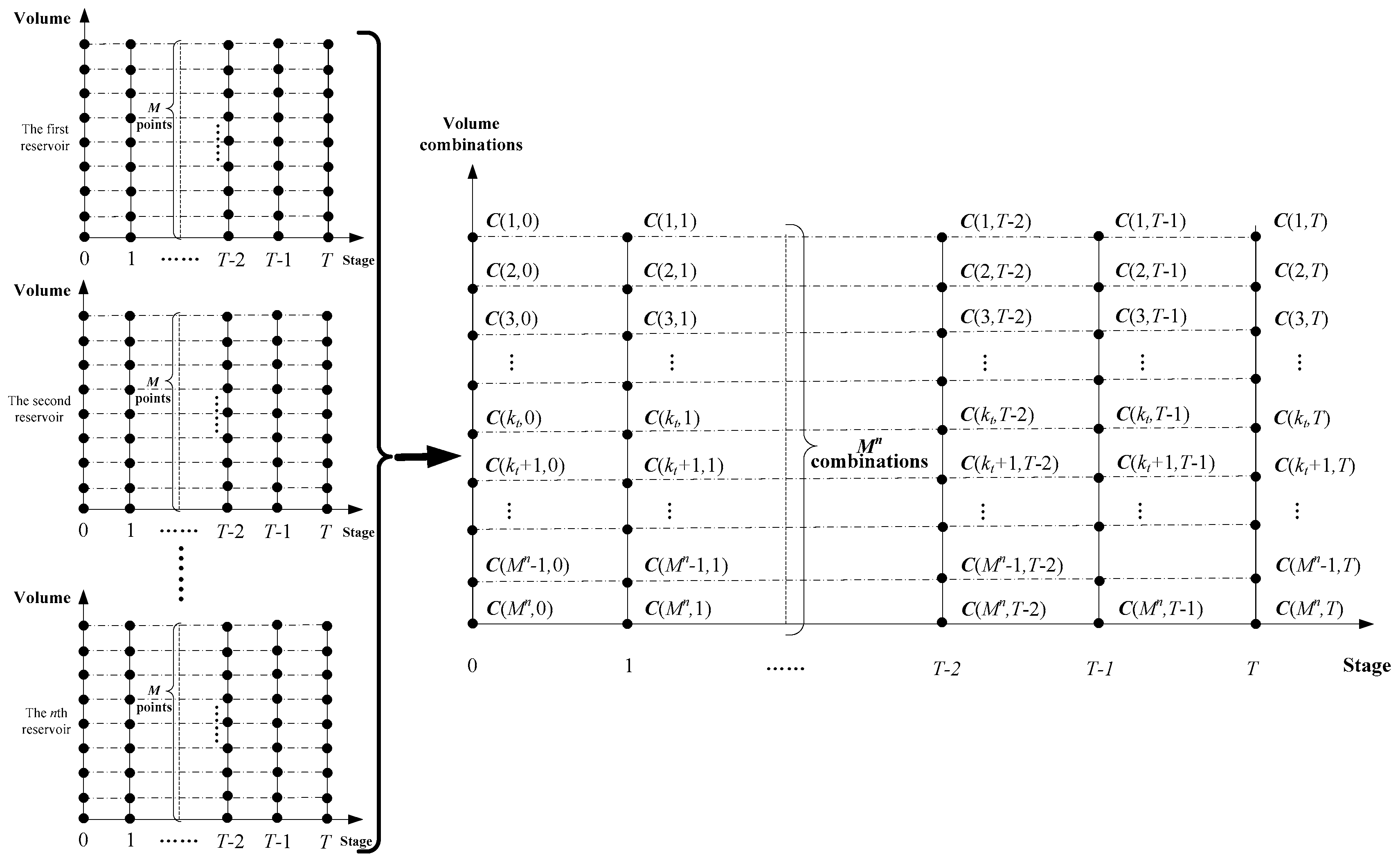
Many variables and constraints are integrated into the procedure of solving a CROO problem, because the number of reservoirs is often two or more in a CROO problem. If the number of discrete points of storage volume for each reservoir is M for a cascade system consisting of n reservoirs, then Mⁿ combinations of these discrete points can be obtained. With reference to the reverse recursion procedure and chronological order recursion procedure of DP in an ROO problem, we can get the optimal combination of storage volume for each stage. Taking a hydropower station system consisting of n reservoirs as an example, the combination principle of discrete storage volume is shown in Figure 1, and the recursive equation of MDP can be formulated as follows.

$$\begin{array}{l}{{\displaystyle F}}_t^{*}\left({{\displaystyle V}}_{t-1}\right)=\underset{{{\displaystyle D}}_t}{\max }\left\{{{\displaystyle N}}_t\left({{\displaystyle V}}_{t-1},{{\displaystyle Q}}_i\right)+{{\displaystyle F}}_{t+1}^{*}\left({{\displaystyle V}}_t\right)\right\}\\ {{\displaystyle F}}_{T+1}^{*}\left({{\displaystyle V}}_T\right)=0\end{array}\}$$

(9)

where ${{\displaystyle Q}}_t^{}$ = (${{\displaystyle Q}}_t^1$,${{\displaystyle Q}}_t^2$,…, ${{\displaystyle Q}}_t^n$)′ is the decision variable vector; and ${{\displaystyle V}}_{t-1}^{}$ = (${{\displaystyle V}}_{t-1}^1$,${{\displaystyle V}}_{t-1}^2$,…, ${{\displaystyle V}}_{t-1}^n$)′ is the state variable vector. In formula (9), because of the discretization, ${{\displaystyle V}}_t^1$ is equivalent to (${{\displaystyle V}}_t^{1,1}$,${{\displaystyle V}}_t^{1,2}$, …, ${{\displaystyle V}}_t^{1,\mathrm{M}}$), ${{\displaystyle V}}_t^2$ is equivalent to (${{\displaystyle V}}_t^{2,1}$,${{\displaystyle V}}_t^{2,1}$,…, ${{\displaystyle V}}_t^{2,\mathrm{M}}$), and ${{\displaystyle V}}_t^n$ is equivalent to (${{\displaystyle V}}_t^{n,1}$,${{\displaystyle V}}_t^{n,2}$,…, ${{\displaystyle V}}_t^{n,\mathrm{M}}$); ${{\displaystyle F}}_t^{*}\left({{\displaystyle V}}_{t-1}\right)$ is the optimal cumulative output of a storage volume combination at the tth stage, unit: kW; and ${{\displaystyle F}}_t^{*}\left({{\displaystyle V}}_t\right)$ is the optimal cumulative output of a storage volume combination at the (t + 1)th stage, unit: kW.

The detailed exposition on the calculation principles and steps of MDP has been recorded in the literature by Ji [37] and Zhang [11].

The POA is a powerful improved dynamic programming in cascade reservoirs operation optimization, which was first proposed by the Canadian researchers N.G. F. Sancho and H. R. Harvson for solving multi-stage dynamic programming problems in 1975. It transforms a complex multi-stage decision problem into a series of two-stage decision-making problems, which simplifies the solution of multi-dimensional problems and decreases their computational complexity. The calculation steps of the POA in solving a CROO model are as follows.

Step 1

Obtain the initial operation trajectories of storage volume by other conventional methods, these can be represented as {${{\displaystyle V}}_0^{}(0)$, ${{\displaystyle V}}_1^{}(0)$,…, ${{\displaystyle V}}_{Mum}^{}(0)$}, where Mum is equal to the number of reservoirs multiplied by the number of operation stages in a year, i.e., Mum = nT.

Step 2

Within the permitted scope, discretize the point ${{\displaystyle V}}_0^{}(0)$, into {${{\displaystyle V}}_0^0(0)$, ${{\displaystyle V}}_0^1(0)$,…,${{\displaystyle V}}_0^M(0)$}, where M is the number of discrete points for an operation point on the initial operation trajectories of storage volume, and the value of the other points on the initial trajectories are fixed.

Step 3

For different discrete points of ${{\displaystyle V}}_0^{}(0)$, which are {${{\displaystyle V}}_0^0(0)$, ${{\displaystyle V}}_0^1(0)$,…, ${{\displaystyle V}}_0^M(0)$}, implement the simulation calculations respectively by using long series runoff data. Find out the point of ${{\displaystyle V}}_0^{*}(0)$ that can maximize the power generation of all operation stages of the cascade reservoirs, then update ${{\displaystyle V}}_0^{}(0)$ with ${{\displaystyle V}}_0^{*}(0)$, and save it as ${{\displaystyle V}}_0^{}(1)$. The power generation in the simulation calculation can be obtained by formula (10), in which k represents the serial number of discrete points

$$E=\max \left\{\left[{{\displaystyle N}}_t^i(k)+{{\displaystyle N}}_{t+1}^i(k)\right]\cdot \Delta t+{\displaystyle \sum _{\begin{array}{l}{i}^{\prime }=1\\ i^{\prime }\ne i\end{array}}^n{\displaystyle \sum _{\begin{array}{l}{t}^{\prime }=1,\\ t^{\prime }\ne t,t+1\end{array}}^T{{\displaystyle N}}_{t^{\prime }}^{i^{\prime }}}\cdot \Delta t;\stackrel{}{}k=1,2,\dots ,M}\right\}$$

(10)

Step 4

In the same way, perform the Steps 2 and 3 to the other points on the initial operation trajectories, and end up with new operation trajectories $\left\{V_0\left(1\right), V_1\left(1\right),\cdots ,V_{Mum}\left(1\right)\right\}$.

Step 5

Compare the power generation between the initial operation trajectories {V₀(0), V₁(0),…, ${{\displaystyle V}}_{Mum}^{}(0)$} and the new operation trajectories {V₀(1), V₁(1),…, V_Mum(1)}; if the error meets the accuracy requirements, then stop counting, otherwise take {V₀(1), V₁(1),…, V_Mum(1)} as the new initial operation trajectories, and repeat Step 2 to Step 4.

3.2. Hybrid Application of MDP and POA

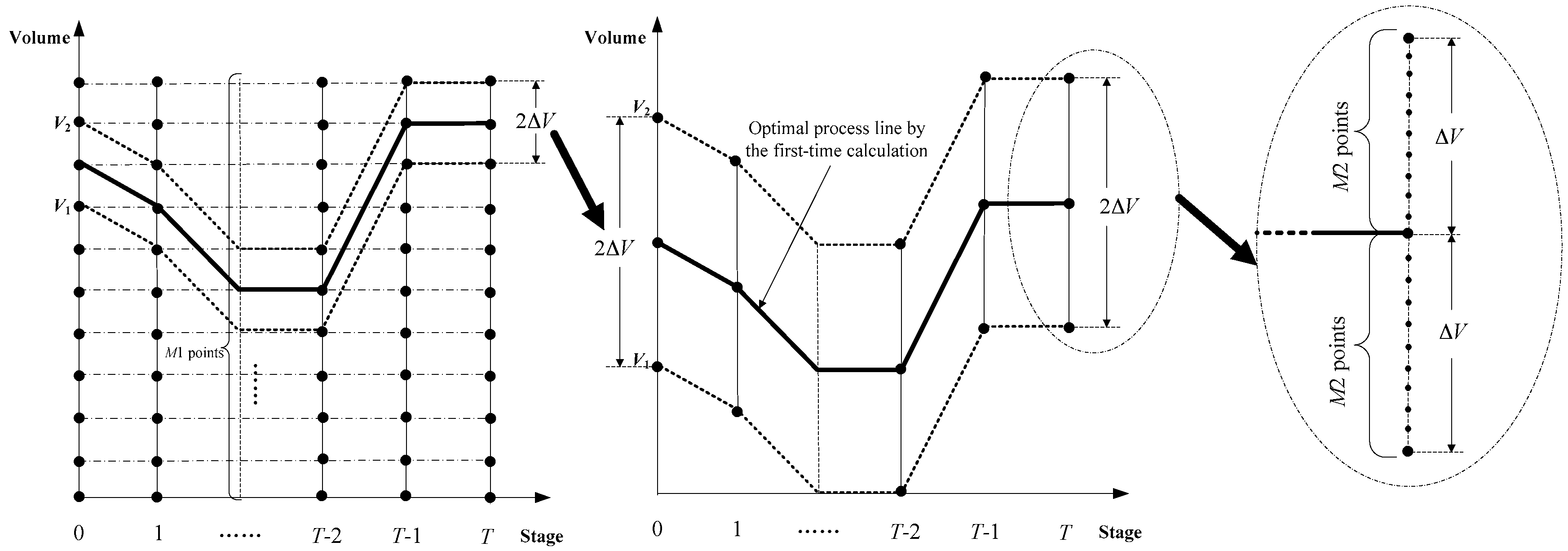
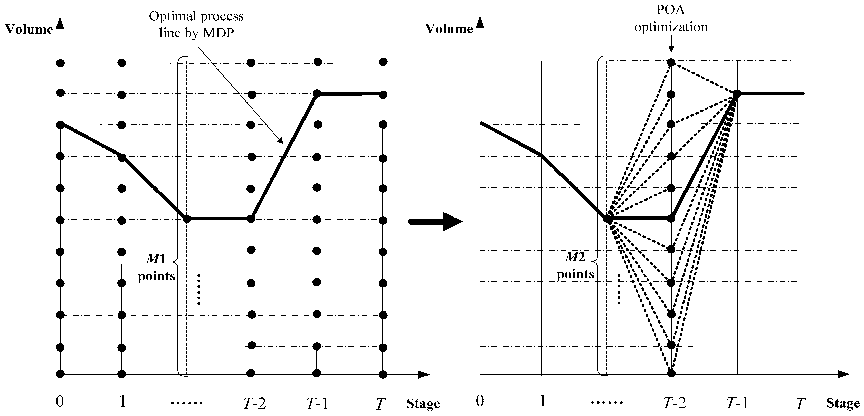
As we know, for a large-scale cascade hydropower system, the calculation amount of MDP in a high discrete degree will be very huge, which can lead to a very long run-time, while in a low discrete degree, it cannot guarantee the accuracy of the final solution. As described the introduction, the POA is sensitive to the initial trajectories, but it has a strong local search ability and fast computing speed. Therefore, if we take the global optimal trajectories of MDP in a low discrete degree as the initial trajectories of the POA, and implement further optimization to the obtained initial trajectories by the POA with a high discrete degree, then we can effectively avoid their defects and play their advantages. That is to say, we first obtain the relatively good initial trajectories for the POA by MDP in a short time, and then optimize the initial trajectories further by the POA, which can give full play to its local search ability and only take a very short time. Described above is the basic principle of the proposed hybrid algorithm in this paper, i.e., MDP-POA.

Taking the optimization calculation of one reservoir as an example, the principle of MDP-POA is shown in Figure 2. For cascade reservoirs, its principle is basically identical to Figure 2. In Figure 2, M1 is the number of discrete points for MDP optimization, and it usually takes a small value, such as 20 or 30. M2 is the number of discrete points for POA optimization, and it usually takes a large value, such as 100 or 200.

The calculation steps of MDP-POA in solving a CROO model are similar to that of the POA. The difference is in the first step, where the POA obtains the initial operation trajectories of the storage volume by conventional methods, but we obtain the initial optimal operation trajectories of the storage volume by MDP with a low discrete degree (such as 10, 20, or 30) in MDP-POA.

3.3. Improved MDP

There is a “curse of dimensionality” problem for MDP, mainly because it is a traversal optimization process, which means that all combinations of storage volume in the feasible region are calculated. The calculation amount of MDP is usually very huge when the number of discrete points is large. However, what we ultimately need is just an optimal storage volume process line; not all the calculations in the traversal optimization are required for us in the end. Therefore, the question of how to reduce the unnecessary calculations is the key to shorten the run-time of MDP. The essence of shortening the run-time for MDP is to reduce the amount of discrete combinations of storage volume in the calculation.

On the whole, there are two ways to decrease the discrete combinations. The first way is to implement the calculation with a low discrete degree, which will reduce the number of total discrete combinations, but it will affect the precision of the final solution. The second way is to implement the calculation with a high discrete degree, but remove the unlikely optimal solution region first. However, the optimal result of MDP in a current discrete degree is related to all of the discrete combination calculations. So, before the traversal calculation, we cannot eliminate any discrete combinations that we think are unlikely optimal solution regions in the calculation, and we can eliminate them only after we make sure of it. Therefore, we can implement the calculation with a low discrete degree first, which is used to determine the generally unlikely optimal solution region in a short time, and remove it, and then implement further optimization for the rest of the region with a relatively high discrete degree, so as to ensure the accuracy of algorithm. The rest of the feasible region mentioned above is actually a corridor constructed through the optimal trajectories of MDP with a low discrete degree, and the further optimization also described above is actually implemented in the corridor by MDP with a relatively high discrete degree. Described above is the basic principle of the proposed improved MDP in this paper, i.e., IMDP.

Taking the optimization calculation of one reservoir as an example, the principle of IMDP is shown in Figure 3. For cascade reservoirs, its principle is basically identical to Figure 3. In Figure 3, the corridor size can be two or more discrete units around the initial optimal trajectories, and the times of corridor optimization can be implemented once or several times.

In contrast, there are two differences between IMDP and Incremental Dynamic Programming (IDP). The first is that IDP requires an initial operation trajectory; however, IMDP directly uses the optimal solution of MDP in a low discrete degree as the initial operation trajectory of MDP in further optimization with a high discrete degree, and it does not need to find the initial solution by other methods. The second is that IMDP generally requires only one-time corridor optimization to achieve a good result, while IDP may require multiple iterations, and so its computation time is generally longer.

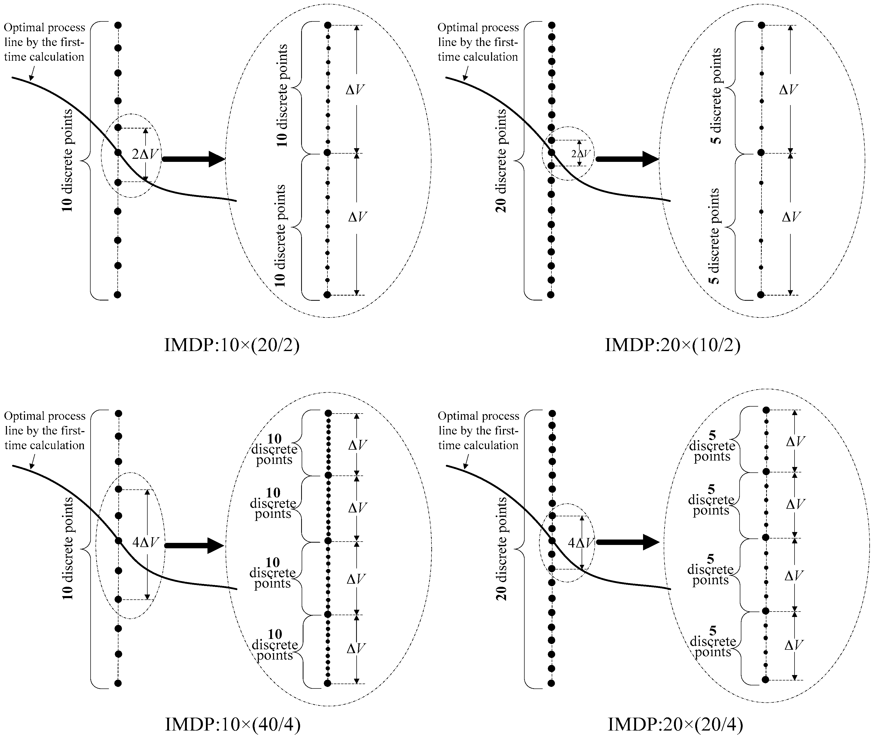
According to the above principle of IMDP, we can construct the corridor by the optimal result of MDP in a low discrete degree (such as 10, 20, or 30), and set up some IMDP schemes, for example, schemes “IMDP: 10 × (20/2)”, “IMDP: 10 × (40/4)”, “IMDP: 20 × (10/2)”, and “IMDP: 20 × (20/4)” as shown in Figure 4, in which the discrete degree of the schemes is equivalent to the discrete degree of MDP with 100 discrete points. Taking the IMDP scheme “IMDP: 10 × (20/2)” for example, it has 10 discrete points in the first-stage calculation and 20 discrete points in the second-stage calculation, and the 20 discrete points are distributed in two discrete units uniformly, which can be demonstrated by the first figure in Figure 4. So, the discrete degree of scheme “MDP: 100” and “IMDP: 10 × (20/2)” are the same, or at least the discrete degree of the IMDP scheme is not lower than that of MDP. The meaning of other IMDP schemes in Figure 4 are similar to scheme “IMDP: 10 × (20/2)”.

The calculation steps of IMDP in solving a CROO model are similar to that of MDP, which can be briefly summarized as follows.

Step 1

Obtain the initial optimal operation trajectories of the storage volume by MDP in a low discrete degree (such as 10, 20, or 30), which can be represented as {${{\displaystyle V}}_0^{}(0)$,${{\displaystyle V}}_1^{}(0)$,…, ${{\displaystyle V}}_{Mum}^{}(0)$}.

Step 2

Construct a corridor through the initial optimal operation trajectories of MDP obtained in Step 1.

Step 3

Within the constructed corridor scope, discretize every point in {${{\displaystyle V}}_0^{}(0)$,${{\displaystyle V}}_1^{}(0)$,…, ${{\displaystyle V}}_{Mum}^{}(0)$} by another discrete degree.

Step 4

In the constructed corridor, obtain the optimal storage volume combination for each stage by MDP with a reverse recursion calculation and a chronological order recursion calculation.

4. Case Study

4.1. Basic Data

The Qingjiang River is one of the main tributaries of Yangtze River below the Three Gorges Dam [46], and its basin area is 17,600 km². Its mean annual rainfall, runoff depth, and annual average discharge are approximately 1460 mm, 876 mm, and 423 m³/s, respectively. The total length of the main stream is 423 km with a hydraulic drop of 1430 m [47]. There are three hydropower stations on the main stream, i.e., Shuibuya, Geheyan, and Gaobazhou from upstream to downstream. Two hydropower stations are under regular operation (i.e., Shuibuya and Geheyan), and thus they are selected as the focus of the research in this paper. The basic parameters of the two hydropower stations are shown in

Table 1. Parameters of the Shuibuya and Geheyan hydropower stations in Qingjiang River.

Items	Unit	Shuibuya	Geheyan
Total storage	108 m3	42	34
Flood control storage	108 m3	5	5
Crest elevation	m	409	206
Normal water level	m	400	200
Flood limited water level	m	391.8	192.2
Install capability	MW	1840	1212
Guaranteed output	MW	310	187
Output coefficient	-	8.5	8.5
Regulation ability	-	Multi-year	Annual

, and the plane sketch map of the Qingjiang River cascade hydropower stations is shown in Figure 5 [48].

The long series runoff data of this cascade system is available from 1959 to 2000, a total of 41 years. For this study, the years of 1967, 1999, and 1975 are selected as the typical wet, normal, and dry years, respectively. The runoff data for each typical year is shown in

Table 2. Typical runoff data for each month in the wet, normal, and dry years (m³/s).

Month	Dry Year		Normal Year		Wet Year
	Shuibuya	Geheyan	Shuibuya	Geheyan	Shuibuya	Geheyan
January	208	69	172	57	244	81
February	228	75	322	106	266	88
March	235	77	426	140	346	114
April	608	200	258	84	761	250
May	1431	471	529	174	912	301
June	1157	381	1772	582	1826	601
July	669	219	1716	563	6193	2036
August	280	93	1800	591	1552	511
September	216	71	541	178	2730	898
October	404	133	2305	758	2452	806
November	398	131	642	212	697	230
December	178	59	427	140	174	57

.

4.2. Results and Analysis

According to the data provided above, we solve the CROO problem described in Section 2 by the proposed MDP-POA and IMDP. In the optimization calculation, the length of the operation stage is set to 10 days, the planning horizon is set to one year, the storage water level at the beginning of the entire planning horizon is set to normal level for each reservoir, and no restrictions are set for the end. The upper limit of the water level for each reservoir is flood-limited water level in flood season and normal level in dry season, and the lower limit for each reservoir is the dead level.

In order to comparatively analyze the dimension reduction effect of MDP-POA and IMDP with the baseline MDP, we established five schemes for MDP, and the number of discrete points for these five schemes is 10, 20, 30, 60, and 100, respectively. Ten, 20, and 30 are the numbers of discrete points for the low discrete degree schemes, which are mainly used to construct the corridor for IMDP or derive the initial trajectories for the POA in MDP-POA. Sixty and 100 are the numbers of discrete points for the high discrete degree schemes, which are mainly used for comparative analysis.

In the optimization calculation of MDP-POA, we took the optimal solution of MDP in a low discrete degree as the initial operation trajectories of the POA, and established 13 schemes in the POA optimization stage. The number of discrete points for each scheme is 10, 20, 30, 40, 60, 80, 100, 120, 140, 160, 200, 300, and 400, respectively. In addition, it is important to note that the number of discrete points used in the POA optimization stage should be greater than that in the MDP optimization stage.

In the optimization calculation of IMDP, we constructed the corridor by the optimal results of MDP in a low discrete degree (i.e., 10, 20, or 30), and set up four IMDP schemes, as shown in Figure 4. The discrete degree of the four schemes is equivalent to the discrete degree of MDP with 100 discrete points.

4.2.1. MDP-POA

The detailed calculation results of MDP and MDP-POA in the dry year, the normal year, and the wet year are shown in

Table 3. Detailed calculation results of MDP and MDP-POA in the dry year.

Number of Discrete Points	MDP		MDP-POA (MDP with 10)		MDP-POA (MDP with 20)		MDP-POA (MDP with 30)
	Time (min)	Power Generation (108 kWh)	Time (min)	Power Generation (108 kWh)	Time (min)	Power Generation (108 kWh)	Time (min)	Power Generation (108 kWh)
10	0.0271	64.6816	-	-	-	-	-	-
20	0.3242	64.7359	0.0375	64.6817	-	-	-	-
30	1.5507	64.7549	0.0391	64.7117	0.3359	64.7359	-	-
40	-	-	0.043	64.7233	0.3364	64.7471	1.5585	64.7549
60	23.3055	64.7711	0.0734	64.7270	0.3419	64.7560	1.5681	64.7594
80	--	--	0.0819	64.7334	0.3551	64.7609	1.5819	64.7622
100	174.1452	64.7745	0.0939	64.7349	0.3679	64.7618	1.5887	64.7670
120	-	-	0.1639	64.7384	0.3931	64.7644	1.5962	64.7673
140	-	-	0.1849	64.7391	0.4051	64.7651	1.6048	64.7677
160	-	-	0.2224	64.7402	0.4157	64.7671	1.6136	64.7679
200	-	-	0.2528	64.7403	0.4191	64.7679	1.6266	64.7698
300	-	-	0.5302	64.7434	0.5221	64.7688	1.6932	64.7709
400	-	-	0.8485	64.7442	0.6271	64.7691	1.8133	64.7722

,

Table 4. Detailed calculation results of MDP and MDP-POA in the normal year.

Number of Discrete Points	MDP		MDP-POA (MDP with 10)		MDP-POA (MDP with 20)		MDP-POA (MDP with 30)
	Time (min)	Power Generation (108 kWh)	Time (min)	Power Generation 108 kWh)	Time (min)	Power Generation (108 kWh)	Time (min)	Power Generation (108 kWh)
10	0.0247	99.5278	-	-	-	-	-	-
20	0.3229	99.6715	0.0356	99.5938	-	-	-	-
30	1.6677	99.6997	0.04	99.6386	0.3317	99.6715	-	-
40	-	-	0.0489	99.6526	0.3390	99.6829	1.6799	99.6997
60	24.8702	99.7149	0.0609	99.6598	0.3453	99.6951	1.6863	99.7074
80	-	-	0.0731	99.6700	0.3541	99.7041	1.6919	99.7150
100	174.893	99.7227	0.0876	99.6726	0.3622	99.7123	1.7078	99.7209
120	-	-	0.0954	99.6776	0.3926	99.7129	1.7384	99.7227
140	-	-	0.1056	99.6779	0.4046	99.7163	1.7411	99.7247
160	-	-	0.117	99.6792	0.417	99.7165	1.7454	99.7251
200	-	-	0.1662	99.6808	0.4389	99.7168	1.7824	99.7261
300	-	-	0.2267	99.6829	0.4953	99.7198	1.8393	99.7272
400	-	-	0.3661	99.6879	0.5954	99.7214	1.9009	99.7288

and

Table 5. Detailed calculation results of MDP and MDP-POA in the wet year.

Number of Discrete Points	MDP		MDP-POA (MDP with 10)		MDP-POA (MDP with 20)		MDP-POA (MDP with 30)
	Time (min)	Power Generation (108 kWh)	Time (min)	Power Generation (108 kWh)	Time (min)	Power Generation (108 kWh)	Time (min)	Power Generation (108 kWh)
10	0.0252	141.9756	-	-	-	-	-	-
20	0.3323	142.1347	0.0315	142.1243	-	-	-	-
30	1.5837	142.1806	0.034	142.1629	0.3497	142.1347	-	-
40	-	-	0.045	142.1748	0.3571	142.1805	1.6003	142.1806
60	23.6526	142.2406	0.0541	142.2023	0.3614	142.1951	1.6139	142.2271
80	-	-	0.0645	142.2081	0.3783	142.2027	1.6217	142.2302
100	176.7312	142.2444	0.0758	142.2128	0.3804	142.2028	1.6336	142.2359
120	-	-	0.0822	142.2135	0.3895	142.2072	1.6409	142.2361
140	-	-	0.1050	142.2153	0.3981	142.2112	1.6511	142.2433
160	-	-	0.1102	142.2225	0.4223	142.2130	1.675	142.2453
200	-	-	0.137	142.2227	0.4439	142.2166	1.6994	142.2483
300	-	-	0.1979	142.2237	0.5276	142.2177	1.7829	142.2494
400	-	-	0.2483	142.2263	0.5546	142.2179	1.8099	142.2512

, respectively, where the term “MDP with 10” in the tables means that the optimization result of MDP with 10 discrete points is used as the initial trajectories of POA in MDP-POA optimization. The meaning of “MDP with 20” and “MDP with 30” are similar to “MDP with 10”. The places with bold font or bold italics font in Table 3, Table 4 and Table 5 are the key points to extract the data for

Table 6. Extracted data of MDP and MDP-POA from Table 3, Table 4 and Table 5.

Year	MDP			MDP-POA
	Number of Discrete Points	Time (min)	Power Generation (108 kWh)	Initial Line	Time1 (min)	Number of Discrete Points	Time2 (min)	Total Time (min)	Power Generation (108 kWh)
Dry year	60	23.3055	64.7711	MDP with 30	1.5507	400	0.2626	1.8133	64.7722
	100	174.1452	64.7745	none	none	none	none	none	none
Normal year	60	24.8702	99.7149	MDP with 20	0.3229	140	0.0817	0.4046	99.7163
				MDP with 30	1.6677	80	0.0242	1.6918	99.7150
	100	174.8930	99.7227	MDP with 30	1.6677	120	0.0707	1.7384	99.7227
Wet year	60	23.6526	142.2406	MDP with 30	1.5837	140	0.0674	1.6510	142.2433
	100	176.7312	142.2444	MDP with 30	1.5837	160	0.0913	1.6749	142.2453

.

Through the detailed calculation results of MDP and MDP-POA in Table 3, Table 4 and Table 5, we can extract the relevant data that can indicate that MDP-POA is superior to MDP (with 60 or 100 discrete points) on power generation, including the initial trajectories, the time consumption for initial trajectories, the number of discrete points for the POA, the total computation time, and the power generation, as shown in Table 6, which is mainly used for contrastive analysis between MDP and MDP-POA.

In Table 6, the “Time1” of MDP-POA column represents the time used to obtain the initial trajectories for POA optimization by MDP, and “Time2” represents the time used in POA optimization. “Total time” is the sum of “Time1” and “Time2”, i.e., the run-time of MDP-POA. Several conclusions can be derived from Table 6, as shown below.

First of all, when we take the calculation results of MDP with 10 discrete points as the initial trajectories of POA, no matter how high the number of discrete points we take in POA optimization, there is no case that the MDP-POA on power generation is better than MDP in a high discrete degree (60 and 100). Thus, it can be seen that the dependency of the POA for the initial trajectories is very strong, and it has a great influence on the final results.

Second, in the dry year, the power generation of MDP with 100 discrete points is 64.7745 × 10⁸ kWh. However, in the optimization results by MDP-POA, there is no case that the power generation is greater than 64.7745 × 10⁸ kWh when we take the results of MDP with 10, 20, and 30 discrete points as the initial trajectories of the POA. So, there is no data for MDP-POA to match the results of MDP with 100 discrete points in the dry year, and they are marked with “none” in Table 6.

However, in the above two cases, although the power generation of MDP-POA is slightly insufficient compared with MDP, the run-time is greatly shortened. In the other cases, when we take the results of MDP with a low discrete degree (20 or 30) as the initial trajectories of the POA, the results of MDP-POA on power generation and run-time are both better than the one-off optimization results by MDP with a high discrete degree (60 or 100). The detailed contrasts are as follows.

Although the increment is small, the power generation of MDP-POA is better than MDP. For example, (1) “64.7722” obtained by MDP-POA is greater than “64.7711” obtained by MDP with 60 discrete points in the dry year, (2) “99.7163” obtained by MDP-POA is greater than “99.7149” obtained by MDP with 60 discrete points in the normal year, (3) “142.2433” obtained by MDP-POA is greater than “142.2406” obtained by MDP with 60 discrete points in the wet year, and (4) “142.2453” obtained by MDP-POA is greater than “142.2444” obtained by MDP with 100 discrete points in the wet year.

On the run-time, the results of MDP-POA are much better than MDP. For example, corresponding to the data in Table 6, it can be seen that 1.8133 is much less than 23.3055 (13 times), 0.4046 is much less than 24.8702 (61 times), 1.6918 is much less than 24.8702 (15 times), 1.7384 is much less than 174.8930 (101 times), 1.6510 is much less than 23.6526 (14 times), and 1.6749 is much less than 176.7312 (105 times). On the whole, the calculation time of MDP can be reduced to about 1/10 to 1/100 of the original by MDP-POA.

Thus, it can be seen that the proposed MDP-POA in this paper has a very good application effect, and it can greatly shorten the run-time of MDP on the premise of ensuring the power generation is not less than MDP. In addition, from Table 6, it can be seen that MDP-POA can obtain a relatively better result when the initial operation trajectories are obtained by MDP with 30 discrete points, which means that when the number of discrete points of MDP is 30, on the one hand, it can be guaranteed that the final result of MD-POA is better than that of MDP, and on the other hand, the calculation time is also stable and within an acceptable range. For the discrete points of POA optimization in MDP-POA, the general value is about 125 when the number of discrete points of MDP is 30, which is the average of 80, 120, 140, and 160 in Table 6.

4.2.2. IMDP

Corresponding to the three typical years, the calculation results of each IMDP scheme are shown in

Table 7. Results of MDP and IMDP.

Dry Year			Normal Year			Wet Year
Scheme	Time (min)	Power Generation (108 kWh)	Scheme	Time (min)	Power Generation (108 kWh)	Scheme	Time (min)	Power Generation (108 kWh)
MDP: 100	174.1452	64.7745	MDP: 100	174.8930	99.7227	MDP:100	176.7312	142.2444
IMDP: 10 × (20/2)	0.4295	64.7552	IMDP: 10 × (20/2)	0.4425	99.6990	IMDP: 10 × (20/2)	0.4285	142.2450
IMDP: 20 × (10/2)	0.3567	64.7738	IMDP: 20 × (10/2)	0.3551	99.7281	IMDP: 20 × (10/2)	0.3635	142.2373
IMDP: 10 × (40/4)	5.8605	64.7752	IMDP: 10 × (40/4)	5.9122	99.7270	IMDP: 10 × (40/4)	5.7351	142.2494
IMDP: 20 × (20/4)	0.7389	64.7746	IMDP: 20 × (20/4)	0.7402	99.7285	IMDP: 20 × (20/4)	0.7337	142.2466

below. The bold font in Table 7 means the power generation of scheme “IMDP: 10 × (20/2)” and “IMDP: 20 × (10/2)” is slightly insufficient compared with scheme “MDP:100”.

In Table 7, the scheme “MDP: 100” is the baseline MDP scheme, which is the one-time calculation mode and means that the MDP has 100 discrete points in the whole calculation. The schemes “IMDP: 10 × (20/2)”, “IMDP: 20 × (10/2)”, “IMDP: 10 × (40/4)”, and “IMDP: 20 × (20/4)” are the IMDP schemes, and they are in the two-time calculation mode.

From Table 7, it can be seen that the results of scheme “IMDP: 10 × (40/4)” and scheme “IMDP: 20 × (20/4)” on run-time and power generation are both better than scheme “MDP: 100” in the dry year, the normal year, and the wet year. Especially on run-time, the superiority of IMDP is significant, as the run-time of “IMDP: 10 × (40/4)” can be reduced to about 1/30 of “MDP: 100”, and the run-time of “IMDP: 20 × (20/4)” can be reduced to about 1/240 of “MDP: 100”.

For the scheme “IMDP: 10 × (20/2)” and the scheme “IMDP: 20 × (10/2)”, although the power generation is slightly insufficient compared with scheme “MDP:100” in some cases (as shown by bold font in Table 7), they are better than scheme “MDP: 100” in most cases, and their superiority is also very significant on run-time, as the run-time of “IMDP: 10 × (20/2)” can be shortened to about 1/400 of “MDP:100”, and the run-time of “IMDP: 20 × (10/2)” can be shortened to about 1/500 of “MDP: 100”.

Therefore, on the whole, the proposed IMDP in this paper can not only greatly shorten the run-time of MDP, but also can effectively guarantee the global convergence of the algorithm. In addition, from the comparison of the four IMDP schemes, it can be seen that the schemes “IMDP: 10 × (40/4)” and “IMDP: 20 × (20/4)” are better than schemes “IMDP: 10 × (20/2)” and “IMDP: 20 × (10/2)”. That is to say, in general, the wider the constructed corridor is in the optimization calculation, the better the final results are at the end. Although the run-time will generally increase with the enlargement of the corridor size, it is still much less than that of MDP. In addition, from the perspective of computing time, comparing the scheme “IMDP: 10 × (40/4)” with the scheme “IMDP: 20 × (20/4)”, it can be found that the computing time of the “IMDP: 10 × (40/4)” scheme is much bigger than that of the “IMDP: 20 × (20/4)” scheme, so the scheme “IMDP: 20 × (20/4)” is superior to “IMDP: 10 × (40/4)”, which indicates that it is best to set the same discrete degree in the two-stage calculation of IMDP when using it to solve a CROO problem, such as the 20 to 20 in scheme “IMDP: 20 × (20/4)”. Such a parameter setting can not only achieve the final expected discrete degree, but also can be very good to avoid the unevenness of the discrete degree in the two-stage calculation of IMDP, which often results in a huge amount of total computation.

Taking the schemes “IMDP: 10 × (40/4)” and “IMDP: 20 × (20/4)” as examples, the storage water level variations of Shuibuya and Geheyan reservoir in the three typical years are shown in Figure 6 and Figure 7, respectively. In the two figures, the “Up reservoir” represents the Shuibuya reservoir, and the “Down reservoir” represents the Geheyan reservoir. The green line (MDP schemes) in Figure 6 and Figure 7 cannot be seen sometimes, because it is covered by the red line (IMDP schemes).

From Table 7, it can be seen that the power generation of IMDP is worse than MDP in some cases. The reason is that the constructed corridor by the calculation result of MDP does not cover the optimal solution of MDP with 100 discrete points. In addition, as we know, MDP has a global convergence which was proved [49], and its calculation results must be the optimal value under a certain discrete degree. However, from Table 7, we can see that the power generation of IMDP is often greater than MDP. The reason for this phenomenon is that there are boundary constraints which make the discrete degree in some parts of the corridor higher than the discrete degree of MDP with 100 discrete points. In fact, for all of the three typical years, this situation often happens in the dry season.

In addition, when comparing the results from this study with the research results in other literature, it can be found that the proposed MDP-POA and IMDP in this paper have a great advantage in computing time. For example, in the literature by Ji et al. [37], the computing time of MNDP is significantly greater than that of MDP, while from the Table 6 and Table 7, it can be found that the computing time of MDP-POA and IMDP are much smaller than that of MDP on the premise of ensuring the quality of solution, which means that the MDP-POA and IMDP have great advantage in computing time compared to the MNDP method. For the parallel MDP provided in the literature by Zhang et al. [11], in solving the joint optimization of two reservoirs with a discrete degree of 48, its computing time of the three kinds of parallel modes is between 2 and 4 min, however, for the IMDP algorithm proposed in this paper, besides the scheme “IMDP: 10 × (40/4)”, the computing time of the rest of the schemes is less than 1 min. Addtionally, it is important to note that the discrete degree of IMDP in this paper is equivalent to 100, whose number of combinations of storage volume is much bigger than that of 48 in the parallel MDP; moreover, IMDP is a serial calculation mode and only one central processing unit (CPU) core is needed in the calculation, while the calculation of the parallel MDP calls over a dozen CPU cores. Therefore, in general, the IMDP proposed in this paper is better than the parallel MDP provided in the literature by Zhang et al. [11].

5. Conclusions

Aiming at the “curse of dimensionality” problem of MDP, this paper proposed two dimension reduction methods after a characteristic analysis of the MDP algorithm, i.e., MDP-POA and IMDP. The Qingjiang cascade reservoirs were selected as a study case, with conclusions summarized as follows.

(1)

The two methods both can greatly shorten the run-time of baseline MDP and effectively hold its optimality to a certain extent. Although the incremental power generation is not significant, the run-time reduction is especially significant; MDP-POA can shorten the run-time to around 1/10 to 1/100 of the baseline MDP, and IMDP can shorten the run-time to around 1/30 to 1/500 of the baseline MDP.

(2)

For MDP-POA, the higher the discrete degree is in the MDP optimization stage, the better the results are by the POA optimization. For IMDP, the wider the constructed corridor is in the optimization calculation, the better the final results are at the end. Although the run-time will generally increase with the augment of the discrete degree or the enlargement of the corridor size, the superiorities of MDP-POA and IMDP are still significant compared with MDP.

(3)

There is little difference on power generation between MDP-POA and IMDP, but on run-time, IMDP is better than MDP-POA.

In most cases, the power generation of MDP-POA and IMDP is better than MDP, but is insufficient in some cases, which indicates that the proposed algorithms still have a certain deficiency. So, there is still a lot of work that needs to be done in the future. For practical application, more advanced improvements and optimization designs for the two algorithms need to be further studied. For the validity of the proposed methods for other reservoirs, more case studies need to be carried out.

References

1. Liu, X.; Luo, Y.; Yang, T.; Liang, K.; Zhang, M.; Liu, C. Investigation of the probability of concurrent drought events between the water source and destination regions of China’s water diversion project. Geophys. Res. Lett. 2015, 42, 8424–8431. [Google Scholar] [CrossRef]
2. Lu, D.; Wang, B.; Wang, Y.; Zhou, H.; Liang, Q.; Peng, Y.; Tony, R. Optimal operation of cascade hydropower stations using hydrogen as storage medium. Appl. Energy 2015, 137, 56–63. [Google Scholar] [CrossRef]
3. Yohannes, G.; Charles, F.; Kenneth, S.; Channing, A. Optimized reservoir operation model of regional wind and hydro power integration case study: Zambezi basin and South Africa. Appl. Energy 2016, 161, 574–582. [Google Scholar]
4. Kumar, S.V.; Singal, S.K. Operation of hydro power plants-a review. Renew. Sustain. Energy Rev. 2017, 69, 610–619. [Google Scholar]
5. Jiang, Z.Q.; Sun, P.; Ji, C.M.; Zhou, J.Z. Credibility theory based dynamic control bound optimization for reservoir flood limited water level. J. Hydrol. 2015, 529, 928–939. [Google Scholar] [CrossRef]
6. Jiang, Z.; Li, A.; Ji, C.; Qin, H.; Yu, S.; Li, Y. Research and application of key technologies in drawing energy storage operation chart by discriminant coefficient method. Energy 2016, 114, 774–786. [Google Scholar] [CrossRef]
7. Jiang, Z.Q.; Ji, C.M.; Sun, P.; Wang, L.P.; Zhang, Y.K. Total output operation chart optimization of cascade reservoirs and its application. Energy Convers. Manag. 2014, 88, 296–306. [Google Scholar] [CrossRef]
8. Sharma, R.N.; Narottam, C.; Veena, S.; Deepika, Y. Decision support system for operation, scheduling and optimization of hydro power plant in Jammu and Kashmir region. Renew. Sustain. Energy Rev. 2015, 43, 1099–1113. [Google Scholar] [CrossRef]
9. Li, F.; Qiu, J. Multi-objective optimization for integrated hydro–photovoltaic power system. Appl. Energy 2016, 167, 377–384. [Google Scholar] [CrossRef]
10. Ma, C.; Lian, J.; Wang, J. Short-term optimal operation of Three-gorge and Gezhouba cascade hydropower stations in non-flood season with operation rules from data mining. Energy Convers. Manag. 2013, 65, 616–627. [Google Scholar] [CrossRef]
11. Zhang, Y.K.; Jiang, Z.Q.; Ji, C.M.; Sun, P. Contrastive analysis of three parallel modes in multi-dimensional dynamic programming and its application in cascade reservoirs operation. J. Hydrol. 2015, 529, 22–34. [Google Scholar] [CrossRef]
12. Zhou, J.; Zhang, Y.; Zhang, R.; Ouyang, S.; Wang, X.; Liao, X. Integrated optimization of hydroelectric energy in the upper and middle Yangtze River. Renew. Sustain. Energy Rev. 2015, 45, 481–512. [Google Scholar] [CrossRef]
13. Raso, L.; Schwanenberg, D.; van de Giesen, N.C.; van Overloop, P.J. Short-term optimal operation of water systems using ensemble forecasts. Adv. Water Resour. 2014, 71, 200–208. [Google Scholar] [CrossRef]
14. Yang, T.; Gao, X.; Sellars, S.; Sorooshian, S. Improving the multi-objective evolutionary optimization algorithm for hydropower reservoir operations in the California Oroville–Thermalito complex. Environ. Model. Softw. 2015, 69, 262–279. [Google Scholar] [CrossRef]
15. Yang, T.; Asanjan, A.; Welles, E.; Gao, X.; Sorooshian, S.; Liu, X. Developing reservoir monthly inflow forecasts using artificial intelligence and climate phenomenon information. Water Resour. Res. 2017, 53, 2786–2812. [Google Scholar] [CrossRef]
16. Li, F.; Shoemaker, C.A.; Wei, J.; Fu, X. Estimating Maximal Annual Energy Given Heterogeneous Hydropower Generating Units with Application to the Three Gorges System. J. Water Resour. Plan. Manag. 2013, 139, 265–276. [Google Scholar] [CrossRef]
17. El Mouatasim, A. Boolean integer nonlinear programming for water multi-reservoir operation. J. Water Resour. Plan. Manag. 2012, 138, 176–181. [Google Scholar] [CrossRef]
18. EI-Keib, A.A.; Ma, H.; Hart, J.L. Environmentally constrained economic dispatch using the Lagrangian relaxation method. IEEE Trans. Power Syst. 1994, 9, 1723–1727. [Google Scholar] [CrossRef]
19. Papageorgiou, L.G.; Fraga, E.S. A mixed integer quadratic programming formulation for the economic dispatch of generators with prohibited operating zones. Electr. Power Syst. Res. 2007, 77, 1292–1296. [Google Scholar] [CrossRef]
20. Eum, H.; Kim, Y.; Palmer, R.N. Optimal Drought Management Using Sampling Stochastic Dynamic Programming with a Hedging Rule. J. Water Resour. Plan. Manag. 2010, 137, 113–122. [Google Scholar] [CrossRef]
21. Shokri, A.; Haddad, O.B.; Marino, M.A. Reservoir operation for simultaneously meeting water demand and sediment flushing: Stochastic dynamic programming approach with two uncertainties. J. Water Resour. Plan. Manag. 2013, 139, 277–289. [Google Scholar] [CrossRef]
22. Momtahen, S.H.; Dariane, A.B. Direct search approaches using genetic algorithms for optimization of water reservoir operating policies. J. Water Resour. Plan. Manag. 2007, 133, 202–209. [Google Scholar] [CrossRef]
23. Zhang, R.; Zhou, J.; Zhang, H.; Liao, X.; Wang, X. Optimal Operation of Large-Scale Cascaded Hydropower Systems in the Upper Reaches of the Yangtze River, China. J. Water Resour. Plan. Manag. 2014, 140, 480–495. [Google Scholar] [CrossRef]
24. Ji, C.M.; Yu, S.; Zhou, T.; Yang, Z.; Liu, F. Application of Ant Colony Algorithm for Hydropower Dispatching Function Optimization. Autom. Electr. Power Syst. 2011, 35, 103–107. [Google Scholar]
25. Deka, P.C.; Chandramouli, V. Fuzzy Neural Network Modeling of Reservoir Operation. J. Water Resour. Plan. Manag. 2009, 135, 5–12. [Google Scholar] [CrossRef]
26. Yuan, W.; Wu, Z. Discussion on application of cooperative coevolution of differential evolution algorithm to optimal operation of cascaded reservoirs. J. Hydroel. Eng. 2012, 31, 39–43. [Google Scholar]
27. Wang, Y.; Zhou, J.; Mo, L.; Zhang, R.; Zhang, Y. Short-term hydrothermal generation scheduling using differential real-coded quantum-inspired evolutionary algorithm. Energy 2012, 44, 657–671. [Google Scholar] [CrossRef]
28. Arnel, G.; Aleš, Z. Short-term combined economic and emission hydrothermal optimization by surrogate differential evolution. Appl. Energy 2015, 141, 42–56. [Google Scholar]
29. Yang, T.; Gao, X.; Sorooshian, S.; Li, X. Simulating California reservoir operation using the classification and regression-tree algorithm combined with a shuffled cross-validation scheme. Water Resour. Res. 2016, 52, 1626–1651. [Google Scholar] [CrossRef]
30. Chu, W.; Yang, T.; Gao, X. Comment on “High-dimensional posterior exploration of hydrologic models using multiple-try DREAM (ZS) and high-performance computing” by Eric Laloy and Jasper A. Vrugt. Water Resour. Res. 2014, 50, 2775–2780. [Google Scholar] [CrossRef]
31. Lu, B.; Li, K.; Zhang, H.; Wang, W.; Gu, H. Study on the optimal hydropower generation of Zhelin reservoir. J. Hydro-Environ. Res. 2013, 7, 270–278. [Google Scholar] [CrossRef]
32. Zhu-Ge, Y.; Xie, P. The application of DDDP method to optimal operation for cascade reservoirs based on state transformation matrix. In Proceedings of the 2010 International Conference on Computational and Information Sciences ICCIS, Chengdu, China, 17–19 December 2010; Volume 2010, pp. 76–80. [Google Scholar]
33. Yang, C.; Chang, L.; Yeh, C.; Chen, C. Multi-objective planning of surface water resources by multi-objective genetic algorithm with constrained differential dynamic programming. J. Water Resour. Plan. Manag. 2007, 133, 499–508. [Google Scholar] [CrossRef]
34. Mathlouthi, M.; Lebdi, F. Use of generated time series of dry events for the optimization of small reservoir operation. Hydrol. Sci. J. 2009, 54, 841–851. [Google Scholar] [CrossRef]
35. Mousavi, S.J.; Karamouz, M.; Menhadj, M.B. Fuzzy-State Stochastic Dynamic Programming for Reservoir Operation. J. Water Resour. Plan. Manag. 2004, 130, 460–470. [Google Scholar] [CrossRef]
36. Zhao, T.; Cai, X.; Lei, X.; Wang, H. Improved Dynamic Programming for Reservoir Operation Optimization with a Concave Objective Function. J. Water Resour. Plan. Manag. 2012, 138, 590–596. [Google Scholar] [CrossRef]
37. Ji, C.M.; Jiang, Z.Q.; Sun, P.; Zhang, Y.K.; Wang, L.P. Research of multi-dimensional dynamic programming based on multi-layer nested structure and its application in cascade reservoirs. J. Water Resour. Plan. Manag. 2015, 141, 1–13. [Google Scholar] [CrossRef]
38. Wu, Y.; Li, T.; Sun, L.; Chen, J. Parallelization of a hydrological model using the message passing interface. Environ. Model. Softw. 2013, 43, 124–132. [Google Scholar] [CrossRef]
39. Glotic, A.; Glotic, A.; Kitak, P.; Pihler, J.; Ticar, I. Parallel Self-Adaptive Differential Evolution Algorithm for Solving Short-Term Hydro Scheduling Problem. IEEE Trans. Power Syst. 2014, 29, 2347–2358. [Google Scholar] [CrossRef]
40. Dias, B.H.; Tomim, M.A.; Marcato, A.L.M.; Ramos, T.P.; Brandi, R.B.S.; Junior, I.C.d.S.; Filho, J.A.P. Parallel computing applied to the stochastic dynamic programming for long term operation planning of hydrothermal power systems. Eur. J. Oper. Res. 2013, 229, 212–222. [Google Scholar] [CrossRef]
41. Li, X.; Wei, J.H.; Li, T.J.; Wang, G.Q.; Yeh, W.W.G. A parallel dynamic programming algorithm for multi-reservoir system optimization. Adv. Water Resour. 2014, 67, 1–15. [Google Scholar] [CrossRef]
42. Tospornsampan, J.; Kita, I.; Ishii, M.; Kitamura, Y. Optimization of a multiple reservoir system operation using a combination of genetic algorithm and discrete differential dynamic programming: A Case study in Mae Klong system, Thailand. Paddy Water Environ. 2005, 3, 29–38. [Google Scholar] [CrossRef]
43. Lantoine, G.; Russell, R. A Hybrid Differential Dynamic Programming Algorithm for Constrained Optimal Control Problems. Part 1: Theory. J. Optim. Theory Appl. 2012, 154, 382–417. [Google Scholar] [CrossRef]
44. Nandalal, K.D.W.; Bogardi, J.J. Dynamic Programming Based Operation of Reservoirs: Applicability and Limits; Cambridge University Press: Cambridge, UK, 2007. [Google Scholar]
45. Lu, H.; Huang, G.; He, L. Inexact rough-interval two-stage stochastic programming for conjunctive water allocation problems. J. Environ. Manag. 2009, 91, 261–269. [Google Scholar] [CrossRef] [PubMed]
46. Du, Z.; Bin, L.; Ling, F.; LI, W.; Tian, W.; Wang, H.; Gui, Y.; Sun, B.; Zhang, X. Estimating surface water area changes using time-series Landsat data in the Qingjiang River Basin, China. J. Appl. Remote Sens. 2012, 6, 1–16. [Google Scholar] [CrossRef]
47. Fu, X.; Li, A.; Wang, L.; Ji, C. Short-term scheduling of cascade reservoirs using an immune algorithm-based particle swarm optimization. Comput. Math. Appl. 2011, 62, 2463–2471. [Google Scholar] [CrossRef]
48. Zhou, Y.; Guo, S.; Liu, P.; Xu, C. Joint operation and dynamic control of flood limiting water levels for mixed cascade reservoir systems. J. Hydrol. 2014, 519, 248–257. [Google Scholar] [CrossRef]
49. Bellman, R. Dynamic Programming; Princeton University Press: Princeton, NJ, USA, 1957. [Google Scholar]
Figure 1. The discretization procedure of cascade reservoirs’ storage volume and their combination rule in Multi-dimensional Dynamic Programming (MDP).
Water 09 00634 g001
Figure 2. Initial operation trajectories derivation and its further optimization by the Progressive Optimality Algorithm (POA) in MDP-POA.
Water 09 00634 g002
Figure 3. Potential optimal solution region derivation and corridor construction of Improved Multi-dimensional Dynamic Programming (IMDP).
Water 09 00634 g003
Figure 4. The construction of four schemes of IMDP with an equivalent discrete degree of 100 points in MDP.
Water 09 00634 g004
Figure 5. Plane sketch map of the Qingjiang cascade hydropower stations.
Water 09 00634 g005
Figure 6. Storage water level variations of scheme “IMDP: 10 × (40/4)”.
Water 09 00634 g006aWater 09 00634 g006b
Figure 7. Storage water level variations of scheme “IMDP: 20 × (20/4)”.
Water 09 00634 g007