A Semi-Analytical Model for the Hydraulic Resistance Due to Macro-Roughnesses of Varying Shapes and Densities


1
Institut de Mécanique des Fluides de Toulouse (IMFT), Université de Toulouse, CNRS, INPT, UPS, 31400 Toulouse, France
2
Institut Nationale des Sciences Appliqués, 24 Bld de la Victoire, 67084 Strasbourg, France
*
Author to whom correspondence should be addressed.
Water 2017, 9(9), 637; https://doi.org/10.3390/w9090637
Submission received: 21 June 2017
/
Revised: 27 July 2017
/
Accepted: 21 August 2017
/
Published: 25 August 2017
(This article belongs to the Special Issue Water Resources and Environmental Fluid Mechanics: From the Glacier to the Lake/Ocean)
Abstract
:A friction model resulting from investigations into macro-roughness elements in fishways has been compared with a broad range of studies in the literature under very different bed configurations. In the context of flood modelling or aquatic habitats, the aim of the study is to show that the formulation is applicable to both emergent or submerged obstacles with either low or high obstacle concentrations. In the emergent case, the model takes into account free surface variations at large Froude numbers. In the submerged case, a vegetation model based on the double-averaging concept is used with a specific turbulence closure model. Calculation of the flow in the roughness elements gives the total hydraulic resistance uniquely as a function of the obstacles’ drag coefficient. The results show that the model is highly robust for all the rough beds tested. The averaged accuracy of the model is about 20% for the discharge calculation. In particular, we obtain the known values for the limiting cases of low confinement, as in the case of sandy beds.
1. Introduction
Hydraulic modelling requires that the friction created by river beds be well characterised. The formulation generally used is the Manning-Strickler formula, which allows a simple calibration of the hydrodynamic models. The limitations of this formulation have been exposed in cases where the sizes of the roughness elements are similar to the water depth (strong confinement), torrential flow [1], vegetated beds [2,3], unsteady flow, or hyperconcentrated flow [4]. To mitigate these problems, many studies have sought to describe experimentally how friction changes with water depth, slope, or Froude number. However, the formulations set out often seem to be limited to their particular domains of investigation [5,6,7] and rarely allow treatment of flow over beds that may be emergent, confined, or completely submerged. Such significant variations in water depth or slopes are common in models of fish habitat, floodplains, or mountain rivers. The hydraulic resistance of a bed comprising macro-roughness elements is dependent on a knowledge of the drag coefficient of each roughness element. Its definition is generally based on the average flow velocity of the entire water column. This means that, in the standard formulation, decreases with increasing water depth. With vegetation models it is possible to define a coefficient based on the velocity around the obstacle. This coefficient is therefore constant and depends only on the shape of the obstacle. However, the complexity of the three dimensional flow within the roughness elements on the bed is still being investigated and is difficult to model using just a single equation. Although the use of a numerical model is an accurate method to estimate friction factor and head loss, it needs a powerful computation machine [8]. The concept of a double-averaging (spatial and temporal) applied to a vegetated bed [2,9,10] has resulted in a better understanding of the turbulent properties of aquatic canopies. Hence, estimating the transport of sediments or nutrients between the bed and the flow has been improved, allowing a better model of the exchanges necessary for ecosystems to work. In parallel with this development, the double average has been used to obtain the hydraulic resistance of the bed, based on the geometric properties of the canopy. The hydraulic resistance is then estimated using empirical [11,12], analytical [13], or numerical computations [14,15]. These formulations require a turbulence closure relationship to ensure that they are universally valid [6,16]. Using a friction model for rock-ramp fishways, Cassan and Laurens [17] obtained a closure relationship dependent solely on the length scales of the canopy. This relationship was based on a large quantity of experimental vegetation data, on macro-roughness elements, and a series of experiments involving steep slopes. The purpose of this article is to show that this relationship also provides an understanding of the hydraulic resistance of the bed with macro-roughness elements having large spatial densities, steep slopes, and significant confinement. The model proposed provides a theoretical basis for explaining and validating the many experimental formulae for river beds characteristic of the flows found in foothill rivers. The strength of the model is a unified framework for submerged and emergent roughness elements. Moreover, the friction model is not only available for flow above vegetation [2,6,13] but also for rock, gravel, and sand beds. To illustrate the ability of the model for various hydraulic conditions, it is applied to experiments that provide the stage-discharge relationship for steep mountains stream [18,19], for flood plains [20], for prediction of the biological response to management actions [21,22], or for river restoration [1].
In this paper, the bed parameters and model equations are presented first. The second step is the calibration of the drag coefficient for each element shape. A validation is carried out with additional experiments and finally we discuss the model implication for engineering practice.
2. Material and Method
2.1. Bed and Model Description
To describe the bed geometry, it is modelled as an arrangement of blocks regularly spaced from each other in the longitudinal () and transverse () directions. The blocks are defined by a characteristic variable facing the flow D (diameter for a circular cylinder) and by their height k. The average water depth is denoted h, while the water depth normalised with respect to the characteristic size is written . So as to be consistent with previous work, the arrangement of blocks is described using the concentration C, which is related to the spatial density ():
where is the element area in the plane divided by ( for a circular cylinder), is the ratio between the element area in the plane, and a the bed area linked to one element ().
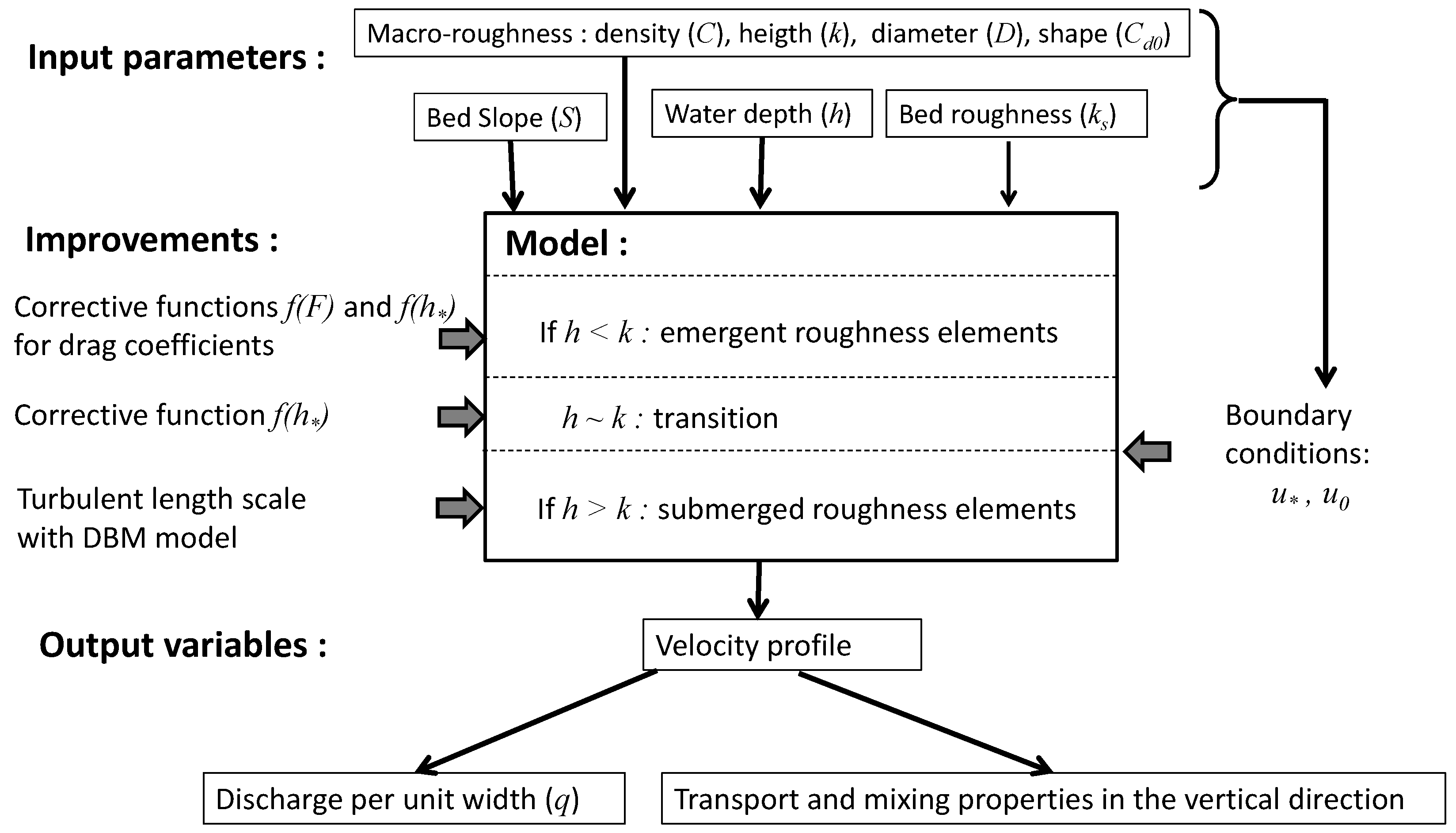
The Figure 1 represents a definition sketch of the velocity profile modeling presented in this study. The specific improvements that it brings, in comparison with previous works, are mentioned. Indeed for emergent macro-roughness, a constant drag coefficient of macro-roughness is not sufficient to reproduce experimental data. Then, the corrective functions proposed by [17] are used and it is shown that they are also relevant to describe the drag force when the elements are just submerged. For water depth higher than the element height, the vertical velocity profile is computed with a one dimension vertical model [14] (hereinafter referred to as the Defina and Bixio Model (DBM)) and a new turbulence closure model.
Table 1 shows the studies used for the drag coefficient calibrations (the first five studies) and the model validation (the following studies). The model is also compared with the empirical formulae specific to rough ramps (Table 2), in particular, the work of [1] with hemispherical macro-roughnesses, which are put on pebbles of characteristic size = 0.019 m.
The formulae from [5,7] are also assessed since they are used frequently. These relationships do not depend on concentration since the obstacles are assumed to be in contact. However, as there is always a space between blocks, the flow can be seen, at least in the upper part, as passing between roughness elements that are highly concentrated. The steep slopes ensure that there is significant turbulent flow in this region.
2.2. Emergent Roughness Elements
Velocity profile and stage-discharge relationship are deduced from the design model for fishways with rough ramps as described in [17]. A uniform flow above a bed comprising macro-roughness elements and bed roughness is assumed here.
If the macro-roughness elements are emergent, and if it is assumed that velocities are vertically uniform [15], the momentum equation can be written in the form [26]:
where is the drag coefficient of the obstacle in the infinitely long case at low Froude number, S is the average slope of the bed, is the Froude number based on the conveyance or bulk velocity , B is the channel width, is the proportion of total area on which bed friction occurs , and is the bed friction coefficient obtained from the formula given by [7,26]. As no bed friction in the wake of an element is considered, is lower than . The expression for is a function of the roughness height of the bed ():
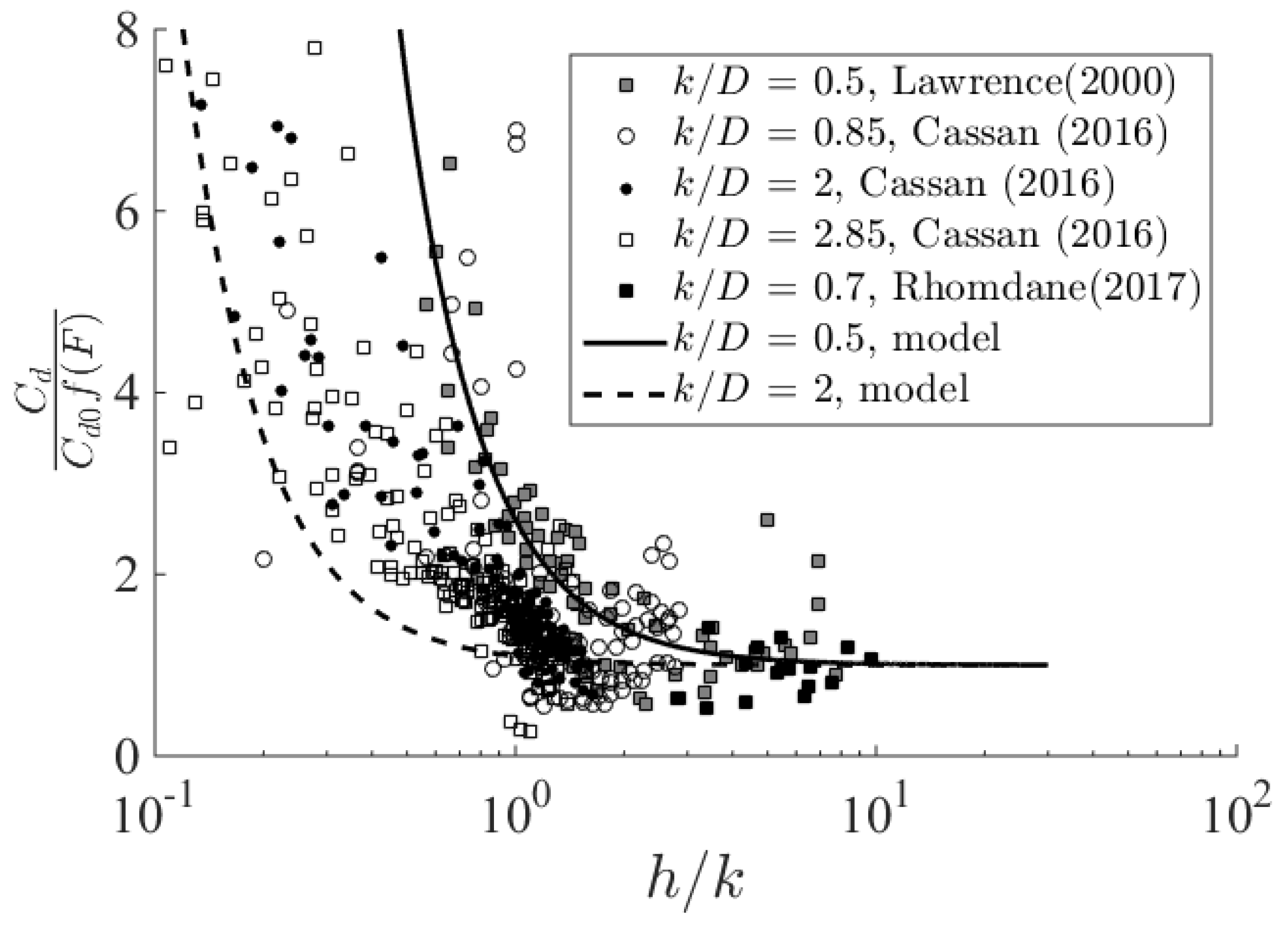
The functions and are due to modification of the free surface and to the interaction between the flow and the bed, respectively. Studies on rock-ramps fishways [17,26,27,28] have provided a better description of these functions experimentally and numerically. They depend on the characteristics of the macro-roughness elements and the conveyance velocity U:
where F is the Froude number based on the velocity and average water depth h between blocks .
Explicitly, the flow rate q per unit width (m) is given for non-submerged roughness elements by the expression:
2.3. Submerged Roughness Elements
For the submerged case, a modified version of the model proposed by [14] is used. This is a model based on the spatial double average and on modeling turbulent stresses via a mixing length. The length assumed here is based on the space available between the roughness elements in the canopy. Following many experiments in fully rough conditions, Cassan and Laurens [17] showed that the turbulent mixing length expressed by Equation (7) enabled the average flow rate and velocity profile to be calculated with good accuracy, both for wide roughness elements (small roughness aspect ratio or shallow layer) or for vegetation (large roughness aspect ratio or deep layer) (Figure 2). In this equation, s is the minimum distance between blocks ().
In the flow layer within and above the macro-roughness elements, turbulent stresses are modeled in two different ways to reflect the different physical phenomena at work (dissipation around the obstacle or a function of the distance from the wall) and are continuous at the top of the canopy. The models used, as well as the expressions for velocity, are summarized in the Table 3.
Continuity of turbulent viscosity allows the turbulence length scale between the macro-roughnesses to be found by means of the relation:
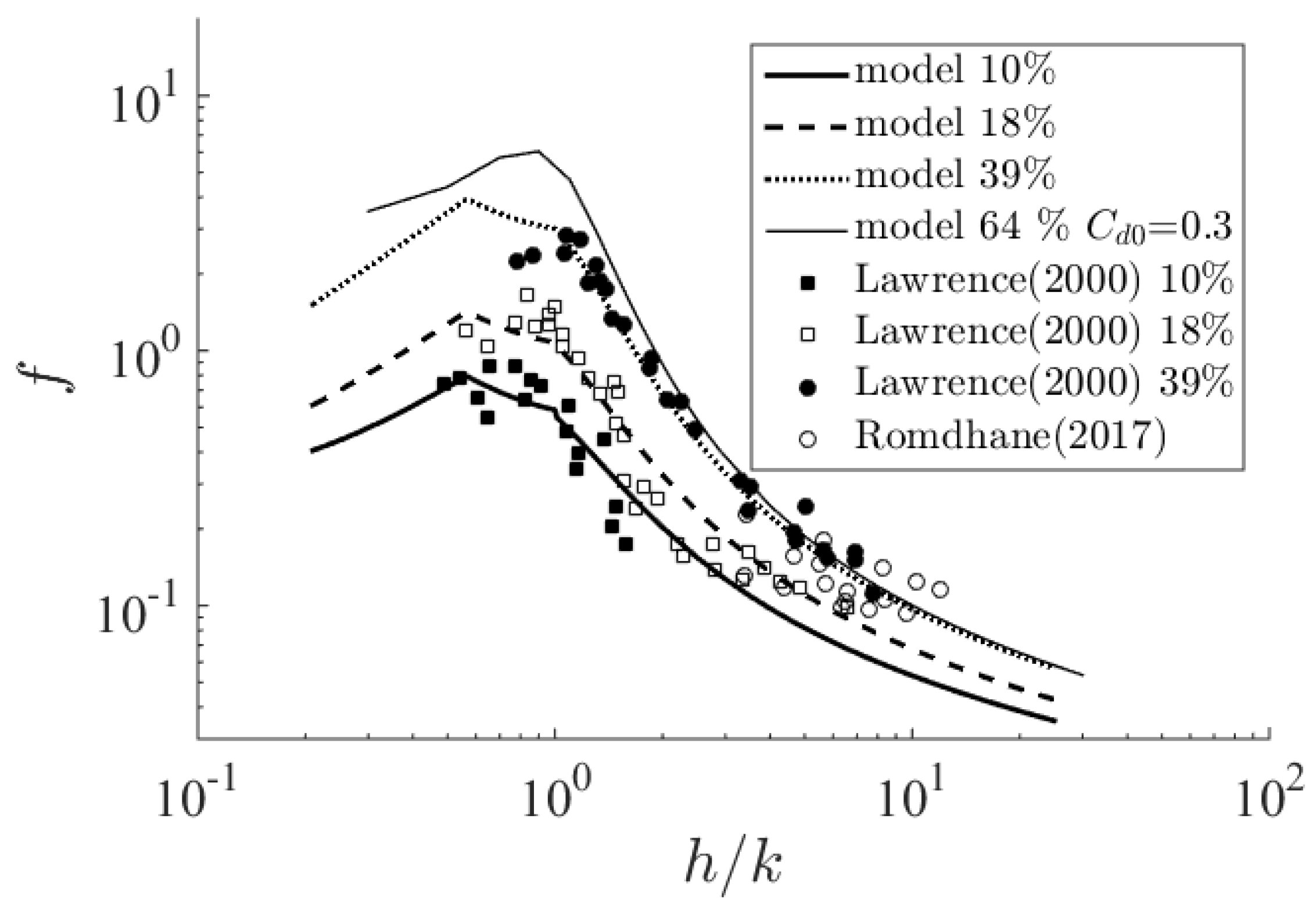
where is the friction velocity and is the velocity at the top of the canopy. The turbulent stress and the friction velocity at the top of the canopy, , are provided by the momentum balance above the roughness elements under uniform steady-state conditions ( ). The velocity at the bed is obtained from the expression defined in the case of emergent roughness elements (Equation (6)), since it is assumed that the turbulence at the bed is zero. Using measured water depths, experimental measurements of were deduced by calibrating our model against the measured flow rate. Dividing by a known value of (see section calibration of drag coefficients) and the function , we obtain the corrector function that best allows our model to reproduce the measured flow rate. We observe in Figure 3 that the function must be used since it enables the transition between the two flow regimes to be estimated.
For the case of large roughness aspect ratio, the contribution from is very small, since is large. For the case of small roughness aspect ratio, there is a continuous transition of the emergent flow influenced by the bed towards a submerged flow. Thus, when h increases this contribution decreases and cancels itself out, meaning that the influence of the bed on the structure of the flow becomes small by comparison with the stress exerted by the upper layer.
As the presence of flow over the element induces a smaller distortion of the free surface, no Froude correction is necessary in the submerged case ( = 1) [29]. This can lead to a slight discontinuity in the model in the emergent-submerged transition but corresponds well with the physical flow changes that are not modeled (i.e., the interaction between the wake cylinder and the free surface deformation).
The velocity profiles can be highly varied depending on the confinement (), concentration (C), drag coefficient , or shape factor () (Figure 4). If is small (<10) the velocity remains fairly uniform and close to that of the bed velocity , which depends on the concentration and on . The validation of the model for this flow can be found in [17]. If is large (>10), the profiles become similar even though the flow rate depends on the drag coefficient of the obstacles. The validation for = 20 is detailed further, in particular in the log law parameters part where parameters for rough bed can be obtained with the model.
3. Results and Discussion
3.1. Calibration of Drag Coefficients
This paper investigates the variant of the DBM model described previously in the case of low aspect ratios and obstacle concentrations C of between 0.05 and nearly 1. Use of the model in cases of vegetation with subcritical flow (F < 0.2) was validated in [17] since the model was able to predict flow rates to an accuracy of better than 20% for circular cylinders with = 1. Here, we focus on other element shapes.
To compare the results, hydraulic resistance will be expressed in terms of the Darcy-Weissbach coefficient defined over the total depth of the flow h.
Where U is the bulk velocity computed by the integration of the velocity profile from Table 3.
The data from [20] (Figure 5) show the continuity of the model since it works for the emergent (), partially, and completely submerged cases even though each behavior is modeled differently ([20]). Compared with the model proposed by [20], where is adjusted using an experimental correlation, we obtain a change in f for the emergent case based on the functions and .
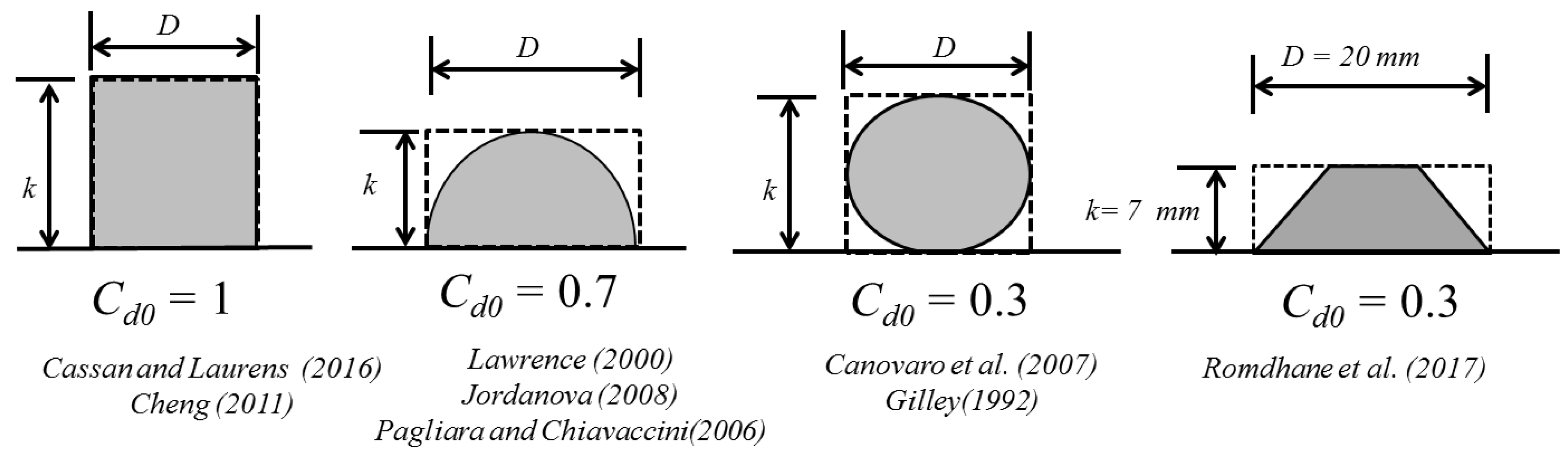
The experimental friction coefficients shown in Figure 5 were obtained by assuming a constant for a given shape of roughness element since the purpose of the model is to provide a friction coefficient that is uniquely a function of the geometrical characteristics of the bed. The values of are 0.7 using the data from [20] obtained from hemispheres and 0.3 using the data from [24] obtained from truncated cones.
The experimental studies cited above used regular roughness elements, however, for applications in the natural environment it is of interest to see how the model is able to adapt to actual bed roughness conditions. To this end, the experimental friction coefficients found by [18] are shown in Figure 6. The roughness elements were ellipsoidally shaped cobbles in concentrations ranging from very low to very high. The height of the roughness element was measured along the smallest axis. Measurements were grouped by range of confinement and compared with the models. Just as for the experiments, we note that f has a little change for C > 0.6; this phenomenon is also reproduced by the model.
The model clearly illustrates how friction depends on concentration, slope, and roughness element size, since a single value of = 0.3 allows fitting with all the series of measurements. It is consistent to find a less than that for a hemisphere ( = 0.7), since here the frontal area facing the flow is smaller. For a given shape of roughness element, D is assumed to be constant and we therefore assume that its change will be taken into account in the value of (Figure 7). Hence, for the same diameter used in the model, the frontal area of the circular cylinder [17] is greater than that of the hemisphere [20], which is itself greater than that of the truncated cone [24]. To a first approximation, the value for ellipsoidal shape appears to correspond to several “cobble” forms of bed roughness element, and it will be taken as the reference for “natural” beds in the remainder of this article.
3.2. Validation of Friction Coefficients for River Flows
In the previous series of measurements (Figure 6), the deviation in f can be as much as 30% but this inconvenience is mitigated by the great robustness of the formula, as the following results show. In particular, a comparison between the average velocities as measured by [18] and the model shows that the flow is estimated with an error of less than 20% ( = 0.59), whatever the concentration considered (Figure 8). Likewise, the measurements obtained by [22] for hemispheres show a similar accuracy even though the difference increases at low average velocities, i.e., for high concentrations. The data from [21] for rigid vegetation () also confirms the validity of the model for circular cylinders.
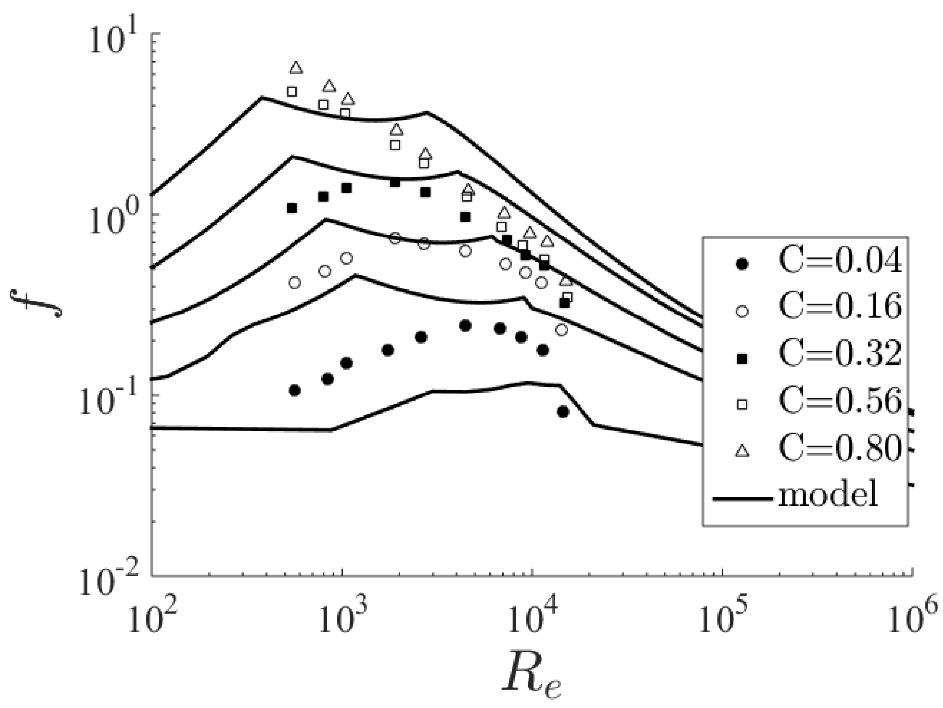
The model is also compared with the results from [23], which are expressed in terms of Reynolds number (Figure 9 and Figure 10). They are a good example of the model validity for emergent-submerged transition and large natural roughness elements. These measurements highlight the need to limit the value of (here < 6) since for values of that are too small, tends to infinity. Indeed, this limitation artificially reproduces bed friction between obstacles where the roughness of the bed between the macro-roughnesses is unknown. For flow above gravel beds, the model accurately reproduces the transition from emergent to submerged (maximum in the experimental data); the error in the friction coefficient is at most 40% and is greatly reduced for emergent flow around large obstacles (Figure 10). For the cobble case, the flow is mostly emergent. The evolution as a function of Reynolds number (and hence of h) and concentration is well reproduced.
The possibility of using the model for beds covered with macro-roughness elements is illustrated by Figure 11. The experimental correlation of [1] gives values of f that agree with our model within the range of applicability of these formulae, i.e., < 10 (Figure 11 (left)) ( = 0.7 because macro-roughness is hemispheric). In particular, the influence of concentration is consistent, and the model estimates the friction for concentrations less than C = 0.3 (here C = 0.1 and C = 0.3), which is the limit of the range of applicability of the formula from [1]. In contrast with the experimental formula, slope plays no part in the friction coefficient, however, this influence remains very small [1,24].
As far as rough ramps are concerned (Figure 11 (right)), i.e., with roughness elements that are more or less contiguous, we observe that the formula of [5] corresponds to a flow with a high obstacle concentration (here with C = 0.5 and = 0.7). This formula appears more suitable than that of [7], which was chosen for fishways because the sizes of the roughness elements on the bed of the fishways were closer to those used in [7]. We may therefore assume that changing the bed friction law might improve the results, especially for low concentrations where the drag is lower.
The formulation proposed by [25] is more generally used in fully rough supercritical flows. It is also close to our predictions in the weakly submerged range, for which it is appropriate. In the emergent case, the friction coefficients are also of the same order of magnitude as our calculation. However, the model takes the concentration into account as well. Generally speaking, the differences between the model and the experiments are less than the orders of magnitude in the differences between the various experimental formulae.
In order to determine the model’s applicability in this range of torrential flows, we tested it on flows with steep slopes and very large roughness elements studied by [19]. The characteristics of the macro-roughness elements and the bed came directly from the average values measured by the author. In order to calibrate the measurements as well as possible, a drag coefficient of = 2 was chosen. This high value is not inconsistent since the blocks can be viewed as emergent plane surface blocks that lead to values of > 1 in emergent cases [26,30]. In Figure 12, small deviations at low (where R is the hydraulic radius equal to h in the model and the characteristic size of the bed roughness) are in fact due to shallow flows where the friction is given by the formula provided by [7]. As we have already pointed out, this formula can be improved to describe the bed. For > 0.5, friction is mainly due to the blocks, and these measurements therefore mean that a single can be used for all sites. We note that the deviations in , and hence in U, are relatively reduced when > 0.5. This remains relatively correct given the simplicity of the friction model and the heterogeneous nature of the roughness elements for each site. It can be seen that the model provides a good calculation of f for sites with different configurations such as at Riedbach, Erlenbach and others [19].
3.3. Log Law Parameters
In order to show the change in velocity profiles as a function of the geometric parameters more clearly, we turn our attention to the parameters d and in the logarithmic law.
The change in as a function of the frontal density (Figure 13) corresponds to that described experimentally for vegetation when is large [31] or for urban canopies [32]. For small , we also get the usual value of k [6] for high concentrations. For very low concentrations, remains constant since depends only on k and not on the confinement . The trend in the experimental results is poorly reproduced for very sparse configurations; these do not correspond with the model assumptions, in particular the spatial average, since dispersive stresses are not taken into account.
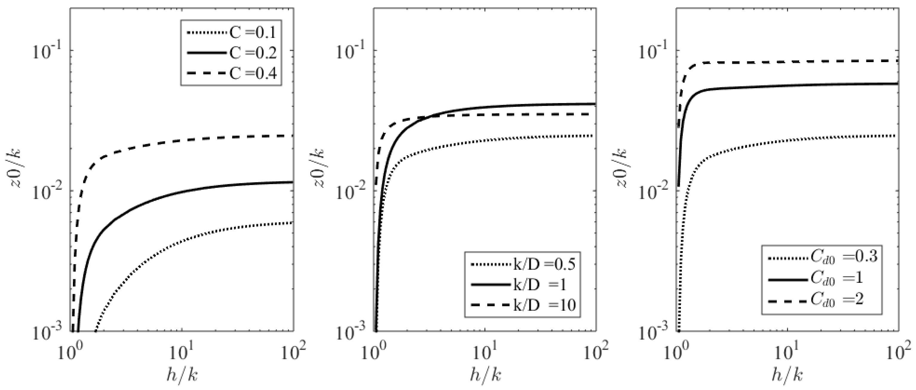
The change in with confinement (Figure 14) shows that while > 10 the hydraulic roughness is independent of water depth or for even smaller values if the roughness elements are sufficiently dense. For example, Ref. [33] could estimate Manning’s roughness coefficient independent of flow depth in a sandy-bed channel where >>10. We find here that the value of depends on the drag coefficient and hence on the form of the roughness elements. This result follows directly from the choice of velocity within the roughness elements (see Table 3, lower layer velocity), which sets the velocity . The hydraulic roughness is written:
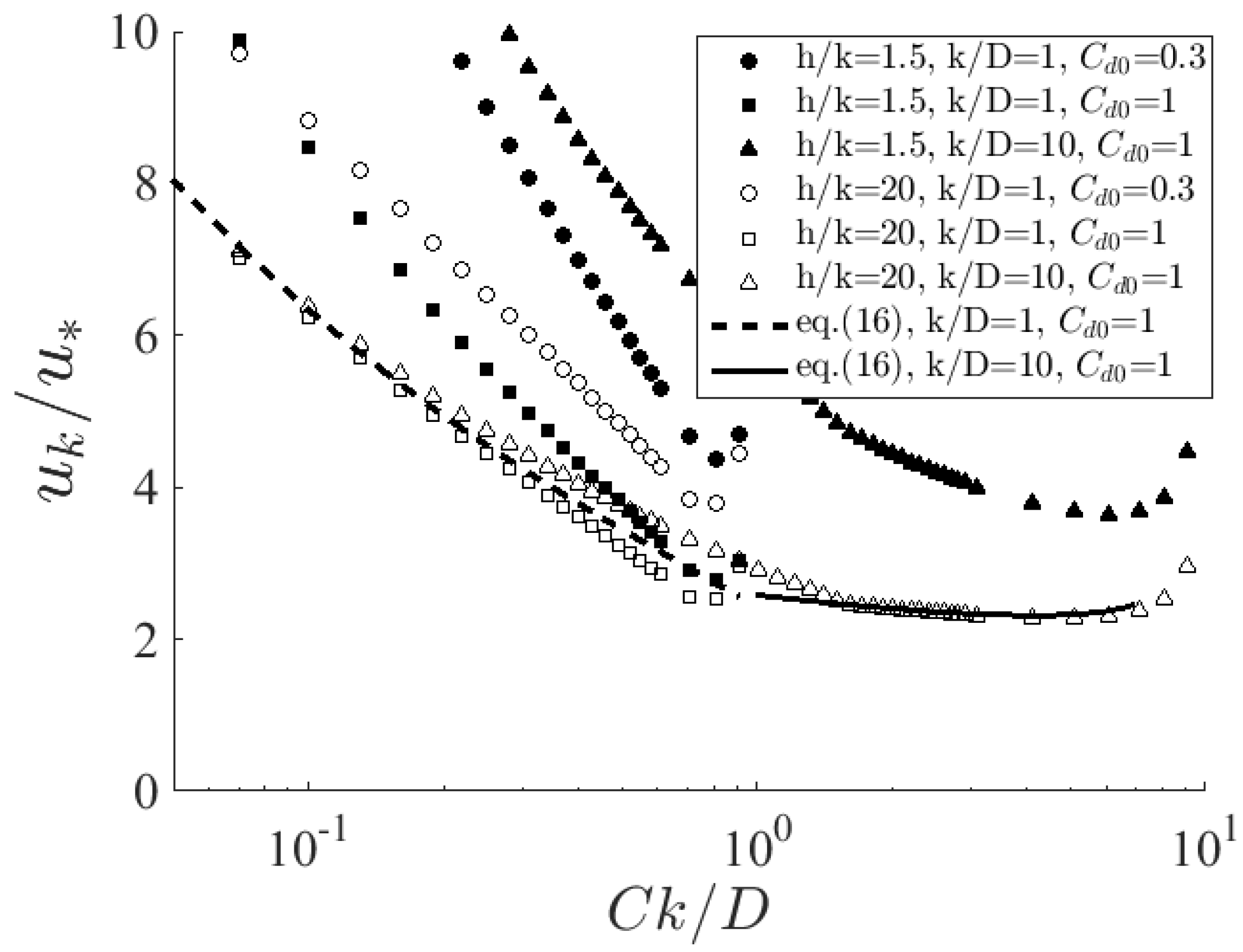
In the case of largely submerged elements, the behavior of can be deduced by calculating the ratio . According to Table 3, the velocity within the roughness elements at the top of the canopy is:
Assuming and neglecting friction at the bed we get:
On the other hand, using the expressions for and , we get for :
For a rough configuration, we find numerically that . Hence, combining the two previous equations (Equations (12) and (13)):
For a small roughness aspect ratio, = 0.15 (Equation (7)), is constant (Equation (16)), and the hydraulic roughness is proportional to the size k of the roughness elements. This result makes our model equivalent to other approaches for this type of roughness element with low confinement ( > 10) [20,34,35].
In cases of a large roughness aspect ratio, depends on concentration (spacing between roughness elements); this explains why, for a fixed concentration, we also find that is constant for large since also tends towards a constant value (Equation (16)).
For both large or small roughness aspect ratio with high confinements ( < 3), Equation (16) no longer holds, and the shape factor then significantly alters the logarithmic law, since can change by an order of magnitude when goes from one to 10. For rough and vegetated beds, this shows the difficulty of unifying the results using other approaches with confinements, since varies greatly.
To focus on the difference between large and small roughness aspect ratio cases, in Figure 15, the hydraulic roughness is given as a function of obstacle density . For densities less than 1, the trend is identical to that identified for atmospheric rough layers [36] even though the results are shifted by a constant dependent on the confinement and shape of the roughness elements. In the case of a large roughness aspect ratio, characteristic of vegetation ( = 10 in the Figure 15), decreases as a function of density as suggested by [31] using concentrations C greater than 0.2. We observe that when the concentration is in the range of 0.4 to 0.9 (bed totally covered) and 1, remains virtually constant and close to the value corresponding to a rough bed (0.03 < < 0.06 for = 20).
Chow [6] showed that a DBM model can be relevant for floods modeling. In their model, the relationship over (Equation (7)) is replacing by an experimental correlation for . The correlation adopted for dense cases and large aspect ratio ( 3) is well reproduced by the present model (Figure 16). The advantage of this work is to complete their study for small aspect ratio and other element shapes.
3.4. Implication for Engineering Practice
The developed model, based on environmental fluid mechanics, allows the computation of the hydraulic resistance for a wide range of flows, from the watershed (hillslope) to the river axis (steep mountains stream and river flow). A single model to predict hydraulic resistance, from the glacier to the ocean, can ease and improve engineering practice for water management at large scale, namely floods, ecological habitat, and sediment transport. To underline this advantage and understand how the model could be applied, a sensitivity study is performed. It also quantifies the accuracy of the data necessary for useful calculations because it is sometimes difficult in the field to identify the form of obstacle considered.
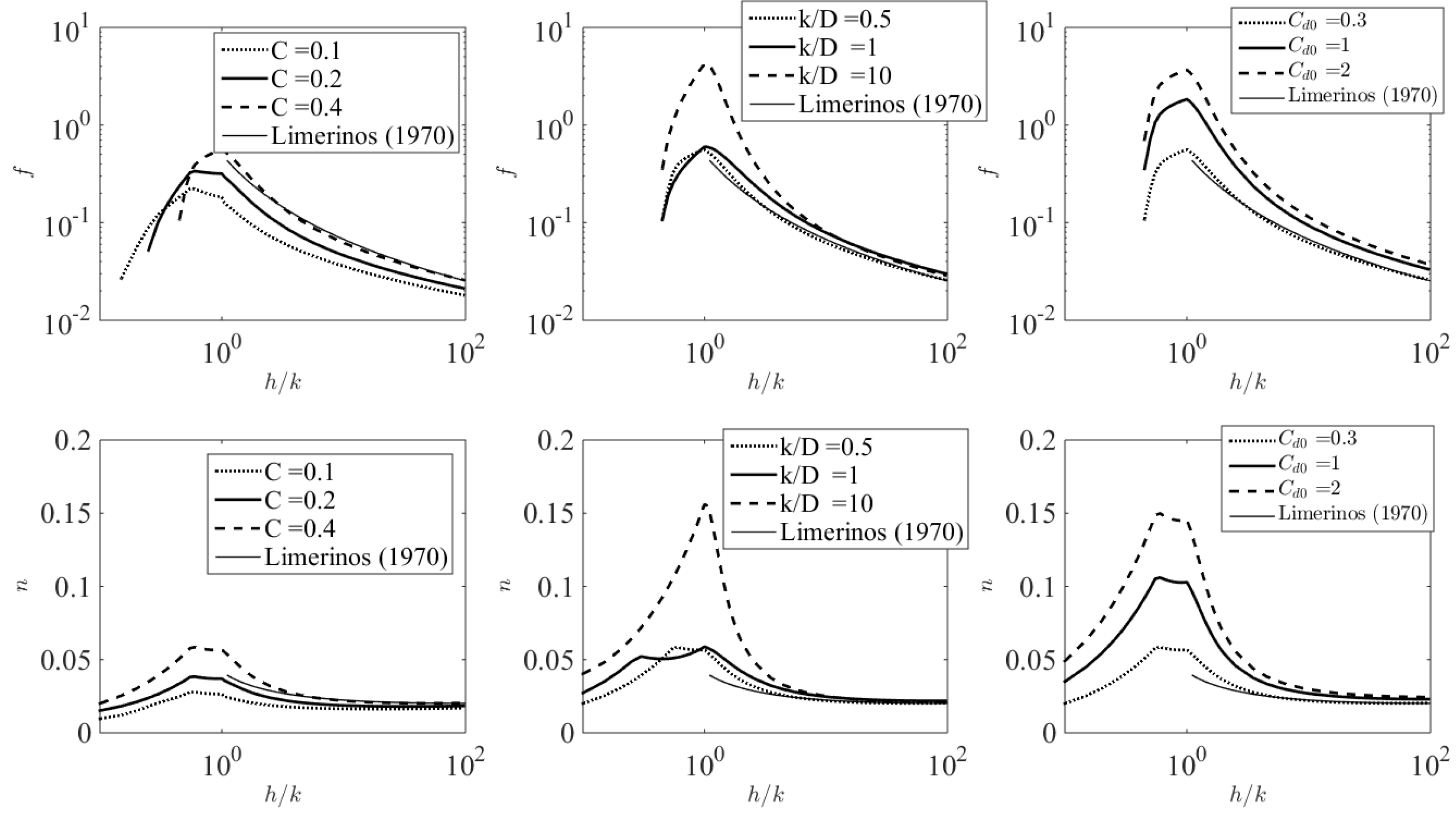
In Figure 17, the friction coefficient is plotted for various values of C, and . The reference values are chosen so as to reproduce the friction on a bed with a high concentration of stony obstacles ( = 0.3 and = 0.5). To this end, the hydraulic resistance is then expressed in terms of the Manning coefficient (Equation (17)), which is more widely used for free surface flows. For a rough bed with < 10, the relationship due to Limerinos [37] (Equation (18)) is appropriate to take into account the influence of .
The model is similar to the Limerinos’ formula when concentration is greater than 0.4 (Figure 17). However, it has the great advantage that it can reproduce an emergent-submerged transition and can take account of forms of obstacle which differs from gravels. We see that for plane faces ( = 2) the friction coefficient is an order of magnitude greater. However, we find that when > 10 the shape of the obstacle makes little difference; this is consistent with the universal applicability of the formula for fully rough walls. In particular, the Manning coefficient changes by only 20% (0.208 and 0.245) in going from a = 0.3 to = 2. For the other parameters in Figure 17, the variation is even smaller. The dominant parameter is therefore the height k of the roughness element, which remains the defining parameter for fully submerged rough beds. Using the Manning coefficient, the expression for friction also shows that in the case of emergent flow this coefficient remains approximately constant. Hence for a simplified use of the model around and above stones, a constant Manning coefficient can be advocated for < 1 and the Limerinos formula for > 1. However, the shape factor has a significant influence whether we take cobbles or rigid vegetation with > 10.
4. Conclusions
In this study, a model was tested in order to reproduce the vertical velocity distribution and the hydraulic resistance of rough beds. Its validity has been demonstrated by comparison with numerous experiments in the literature. Although a maximum difference of 30% could be observed, this error is of the same order of magnitude as that used in practice, for instance by choosing a Manning roughness of n = 0.05 instead of n = 0.04. The robustness is the main advantage of the model. It takes account of the influence of concentration, the height of the roughness elements and the water depth and enables:
- The friction for emergent or submerged roughness elements to be obtained in a continuous sense, which can arise when modeling obstacles in a main channel that are steeply sloping or very cluttered.
- The inclusion of the shape factor for blocks. Indeed, not taking it into account can lead to serious errors when modeling emergent obstacles. In the proposed model, both rocky blocks and vegetation (large ) can be represented as, for example, plantations of trees in a floodplain or overland flows for hillslope hydrology.
- The inclusion of the concentration of obstacles that can be determined in the field or by remote sensing.
- A continuous trend towards “rough bed” formulae when there is a high degree of submergence.
- A calibration parameter to be provided that depends only on the shape of the obstacle.
We have also been able to show that for flow over pebbly beds, the use of Limerinos’ formula [37] in the submerged case could be coupled with a constant value of Manning coefficient in the emergent case to produce a simple, continuous friction model.
Author Contributions
Ludovic Cassan and Hélène Roux proposed the methodology and choose studies for comparison. Ludovic Cassan performed calculations and calibrations. Ludovic Cassan and Hélène Roux analyzed results. Ludovic Cassan, Pierre-André Garambois and Hélène Roux wrote the paper.
Conflicts of Interest
The authors declare no conflict of interest.
References
- Pagliara, S.; Chiavaccini, P. Flow resistance of rock chutes with protruding boulders. J. Hydraul. Eng. 2006, 132, 545–552. [Google Scholar] [CrossRef]
- Klopstra, D.; Barneveld, H.; van Noortwijk, J.; van Velzen, E. Analytical model for hydraulic resistance of submerged vegetation. In Proceedings of the 27th IAHR Congress, San Francisco, CA, USA, 10–15 August 1997; pp. 775–780. [Google Scholar]
- Nepf, H.M. Drag, turbulence, and diffusion in flow through emergent vegetation. Water Resour. Res. 1999, 35, 479–489. [Google Scholar] [CrossRef]
- Chow, V.T. Open-Channel Hydraulics; McGraw-Hill: New York, NY, USA, 1995. [Google Scholar]
- Bathurst, J. Flow resistance estimation in mountain rivers. J. Hydraul. Eng. ASCE 1985, 111, 625–641. [Google Scholar] [CrossRef]
- Katul, G.G.; Poggi, D.; Ridolfi, L. A flow resistance model for assessing the impact of vegetation on flood routing mechanics. Water Resour. Res. 2011, 47, W08533. [Google Scholar] [CrossRef]
- Rice, C.E.; Kadavy, K.C.; Robinson, K.M. Roughness of loose rock riprap on steep slopes. J. Hydraul. Eng.-ASCE 1998, 124, 179–185. [Google Scholar] [CrossRef]
- Calomino, F.; Tafarojnoruz, A.; De Marchis, M.; Gaudio, R.; Napoli, E. Experimental and numerical study on the flow field and friction factor in a pressurized corrugated pipe. J. Hydraul. Eng. 2015, 141, 04015027. [Google Scholar] [CrossRef]
- Lopez, F.; Garcia, M. Mean flow and turbulence structure of open-channel flow through non-emergent vegetation. J. Hydraul. Eng. 2001, 127, 392–402. [Google Scholar] [CrossRef]
- Nikora, N.; Nikora, V.; ODonoghue, T. Velocity profiles in vegetated open-channel flows: Combined effects of multiple mechanisms. J. Hydraul. Eng. 2013, 139, 1021–1032. [Google Scholar] [CrossRef]
- Huthoff, F.; Augustijn, D.C.M.; Hulscher, S.J. Analytical solution of the depth-averaged flow velocity in case of submerged rigid cylindrical vegetation. Water Resour. Res. 2007, 43. [Google Scholar] [CrossRef]
- Konings, A.G.; Katul, G.G.; Thompson, S.E. A phenomenological model for the flow resistance over submerged vegetation. Water Resour. Res. 2012, 48, W02522. [Google Scholar] [CrossRef]
- Meijer, D.G.; Van Velzen, E. Prototype scale flume experiments on hydraulic roughness of submerged vegetation. In Proceedings of the 28th International IAHR Conference, Graz, Austria, 22–27 August 1999. [Google Scholar]
- Defina, A.; Bixio, A. Mean flow and turbulence in vegetated open channel flow. Water Ressour. Res. 2005, 41, 1–12. [Google Scholar] [CrossRef]
- Huai, W.; Zeng, Y.; Xu, Z.; Yang, Z. Three-layer model for vertical velocity distribution in open channel flow with submerged rigid vegetation. Adv. Water Res. 2009, 32, 487–492. [Google Scholar] [CrossRef]
- Poggi, D.; Krug, C.; Katul, G.G. Hydraulic resistance of submerged rigid vegetation derived from first-order closure models. Water Resour. Res. 2009, 45, W10442. [Google Scholar] [CrossRef]
- Cassan, L.; Laurens, P. Design of emergent and submerged rock-ramp fish passes. Knowl. Manag. Aquat. Ecosyst. 2016, 417, 45. [Google Scholar] [CrossRef]
- Canovaro, F.; Paris, E.; Solari, L. Effects of macro-scale bed roughness geometry on flow resistance. Water Resour. Res. 2007, 43, W10414. [Google Scholar] [CrossRef]
- Nitsche, M. Macro-Roughness, Flow Resistance and Sediment Transport in Steep Mountain Streams. Ph.D. Thesis, ETH Zurich, Zurich, Switzerland, 2012. [Google Scholar]
- Lawrence, D.S. Hydraulic resistance in overland flow during partial and marginal surface inundation: Experimental observations and modeling. Water Resour. Res. 2000, 36, 2381–2393. [Google Scholar] [CrossRef]
- Cheng, N. Representative roughness height of submerged vegetation. Water Resour. Res. 2011, 47, W08517. [Google Scholar] [CrossRef]
- Jordanova, A. Low Flow Hydraulics in Rivers for Environmental Applications in South Africa. Ph.D. Thesis, University of the Witwatersrand, Johannesburg, South Africa, 2008. [Google Scholar]
- Gilley, E.; Kottwitz, E.; Wieman, G. Darcy-weisbach roughness coefficients for gravel and cobble surfaces. J. Irrig. Drain. Eng. 1992, 118, 104–112. [Google Scholar] [CrossRef]
- Romdhane, H.; Soualmia, A.; Cassan, L.; Masbernat, L. Evolution of flow velocities in a rectangular channel with homogeneous bed roughness. Int. J. Eng. Res. 2017, 6, 120–128. [Google Scholar]
- Ferguson, R. Flow resistance equations for gravel- and boulder-bed streams. Water Resour. Res. 2007, 43, W05427. [Google Scholar] [CrossRef]
- Cassan, L.; Tien, T.; Courret, D.; Laurens, P.; Dartus, D. Hydraulic resistance of emergent macroroughness at large froude numbers: Design of nature-like fishpasses. J. Hydraul. Eng. 2014, 140, 04014043. [Google Scholar] [CrossRef]
- Ducrocq, T.; Cassan, L.; Chorda, J.; Roux, H. Flow and drag force around a free surface piercing cylinder for environmental applications. Environ. Fluid Mech. 2017, 17, 629–645. [Google Scholar] [CrossRef]
- Tran, T.D.; Chorda, J.; Laurens, P.; Cassan, L. Modelling nature-like fishway flow around unsubmerged obstacles using a 2d shallow water model. Environ. Fluid Mech. 2016, 16, 413–428. [Google Scholar] [CrossRef] [Green Version]
- Sadeque, M.; Rajaratnam, N.; Loewen, M. Flow around Cylinders in Open Channels. J. Eng. Mech. 2009, 134, 60–71. [Google Scholar] [CrossRef]
- Baki, A.; Zhu, D.; Rajaratnam, N. Flow Simulation in a Rock-Ramp Fish Pass. J. Hydraul. Eng. ASCE 2016, 142. [Google Scholar] [CrossRef]
- Luhar, M.; Rominger, J.; Nepf, H. Interaction between flow, transport and vegetation spatial structure. Environ. Fluid Mech. 2008, 8, 423–439. [Google Scholar] [CrossRef]
- Cheng, H.; Hayden, P.; Robins, A.; Castro, I. Flow over cube arrays of different packing densities. J. Wind Eng. Ind. Aerodyn. 2007, 95, 715–740. [Google Scholar] [CrossRef]
- Dodaro, G.; Tafarojnoruz, A.; Sciortino, G.; Adduce, C.; Calomino, F.; Gaudio, R. Modified Einstein sediment transport method to simulate the local Scour evolution downstream of a rigid bed. J. Hydraul. Eng. ASCE 2016, 142. [Google Scholar] [CrossRef]
- Nikuradse, J. Laws of Flow in Rough Pipes; National Advisory Committee for Aeronautics: Washington, DC, USA, 1933. [Google Scholar]
- Raupach, M.R.; Antonia, R.A.; Rajagopalan, S. Rough-wall turbulent boundary layers. Appl. Mech. Rev. 1991, 44, 1–25. [Google Scholar]
- Raupach, M.R.; Hughes, D.E.; Cleuch, H.A. Momentum absorption in rough-wall boundary layers with sparse roughness elements in ramdom and clustered distributions. Bound.-Lay. Meteorol. 2006, 120, 201–218. [Google Scholar]
- Limerinos, J. Determination of the Manning Coefficient from Measured Bed Roughness in Natural Channels; U.S. Geoeological Survey: Tacoma, WA, USA, 1970.
Figure 1.
Definition sketch of the input, output, and improvements of the model. S is the bed slope and the bed roughness heigth.
Figure 1.
Definition sketch of the input, output, and improvements of the model. S is the bed slope and the bed roughness heigth.

Figure 2.
Turbulent length scale as a function of canopy aspect ratio (a) and vertical profile of velocity and turbulent scale for submerged flow (b).
Figure 2.
Turbulent length scale as a function of canopy aspect ratio (a) and vertical profile of velocity and turbulent scale for submerged flow (b).
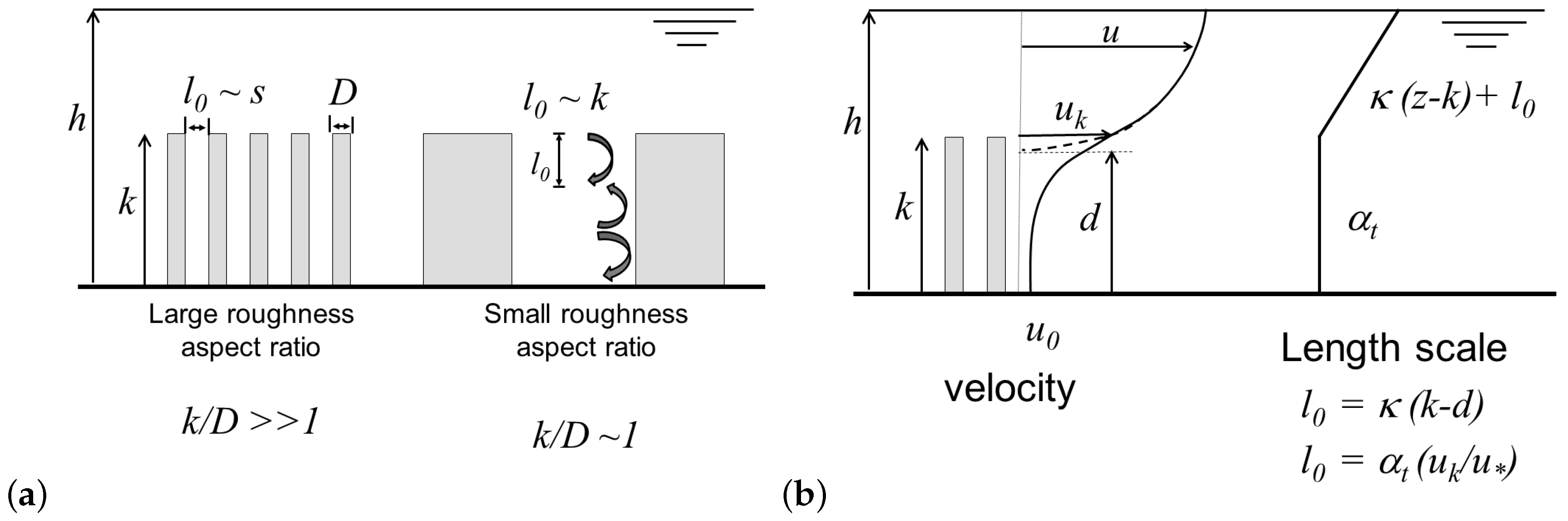
Figure 3.
Experimental corrective function from [20,24] compared with the proposed correlation (Equation (5)).

Figure 4.
Velocity profiles from model as a function of hydraulic and geometrical parameters for weak and high confinement cases (C = 0.2).
Figure 4.
Velocity profiles from model as a function of hydraulic and geometrical parameters for weak and high confinement cases (C = 0.2).

Figure 5.
Friction coefficient from [20,24] and those computed with the present model ( = 0.75, = 0.89, = 0.91, = 0.40).

Figure 6.
Friction coefficients from [18] for randomly spatialized obstacles as a function of the concentration, in comparison to the present model results ( = 1.1, 1.5, 2, 3).
Figure 6.
Friction coefficients from [18] for randomly spatialized obstacles as a function of the concentration, in comparison to the present model results ( = 1.1, 1.5, 2, 3).
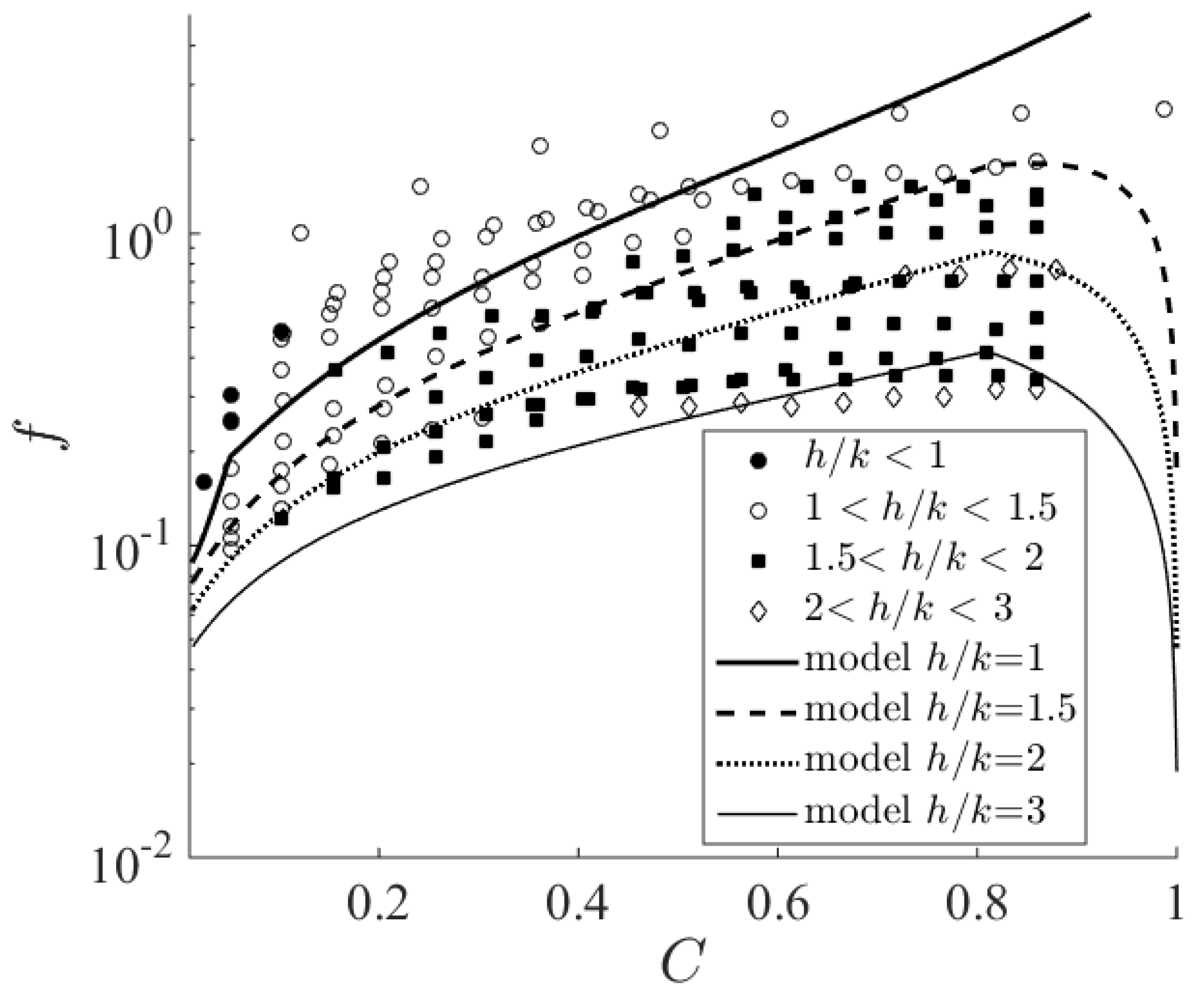
Figure 7.
Comparison of roughness elements with the model assumption, i.e., vertically constant diameter D.
Figure 7.
Comparison of roughness elements with the model assumption, i.e., vertically constant diameter D.

Figure 8.
Comparison between the model and the experimental bulk velocity from [18] ( = 0.3), = 0.59 (a), from [22] ( = 0.7) , 0.78 and from [21] ( = 1) (b). The series correspond to various slopes, diameters, and concentrations tested in each study.
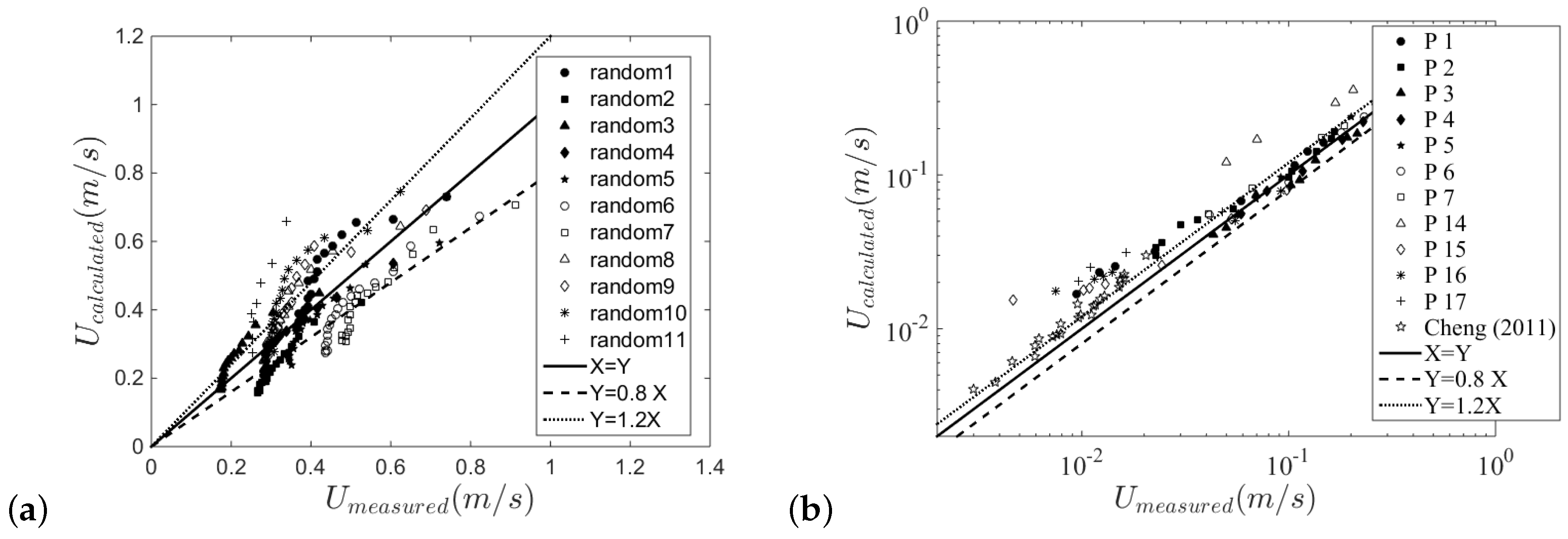
Figure 9.
Friction factor as a function of Reynolds number compared with the experiments of [23] (gravels). The diameter and height are equal to the mean diameter D = k = 0.03 m for randomly spatialized obstacles with fixed concentration.
Figure 9.
Friction factor as a function of Reynolds number compared with the experiments of [23] (gravels). The diameter and height are equal to the mean diameter D = k = 0.03 m for randomly spatialized obstacles with fixed concentration.

Figure 10.
Friction factor as a function of Reynolds number compared with the experiments of [23] (cobbles). The diameter and height are equal to the mean diameter D = k = 0.2 m.
Figure 10.
Friction factor as a function of Reynolds number compared with the experiments of [23] (cobbles). The diameter and height are equal to the mean diameter D = k = 0.2 m.
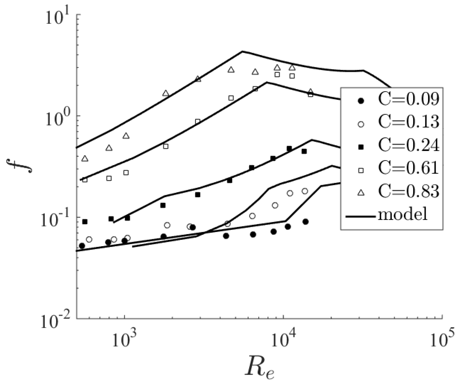
Figure 11.
Comparison between the model and experimental correlations for rock ramps and steep slope. For the model = 0.5 and = 0.7 deduced from analyzed experiments above [20].
Figure 11.
Comparison between the model and experimental correlations for rock ramps and steep slope. For the model = 0.5 and = 0.7 deduced from analyzed experiments above [20].
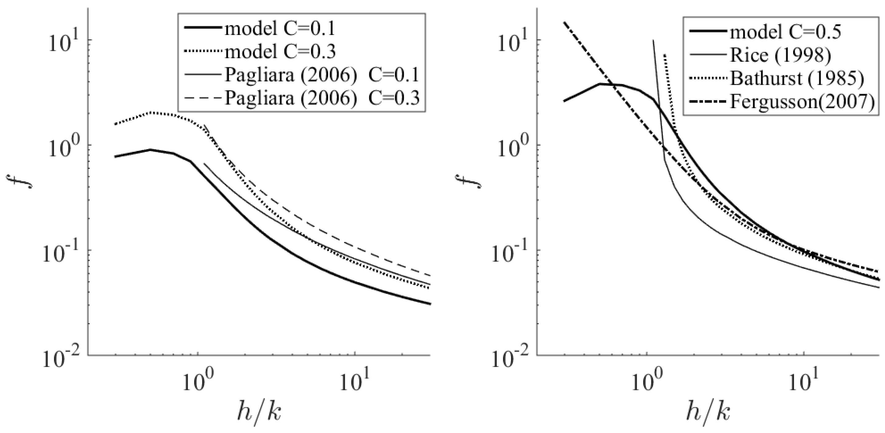
Figure 12.
Hydraulic resistance of real boulders for steep slope rivers. Data from [19] for sites with different configuration, comparison with the present model.
Figure 12.
Hydraulic resistance of real boulders for steep slope rivers. Data from [19] for sites with different configuration, comparison with the present model.

Figure 13.
Displacement height as a function of the frontal density and compared to experimental correlation from [31].
Figure 13.
Displacement height as a function of the frontal density and compared to experimental correlation from [31].
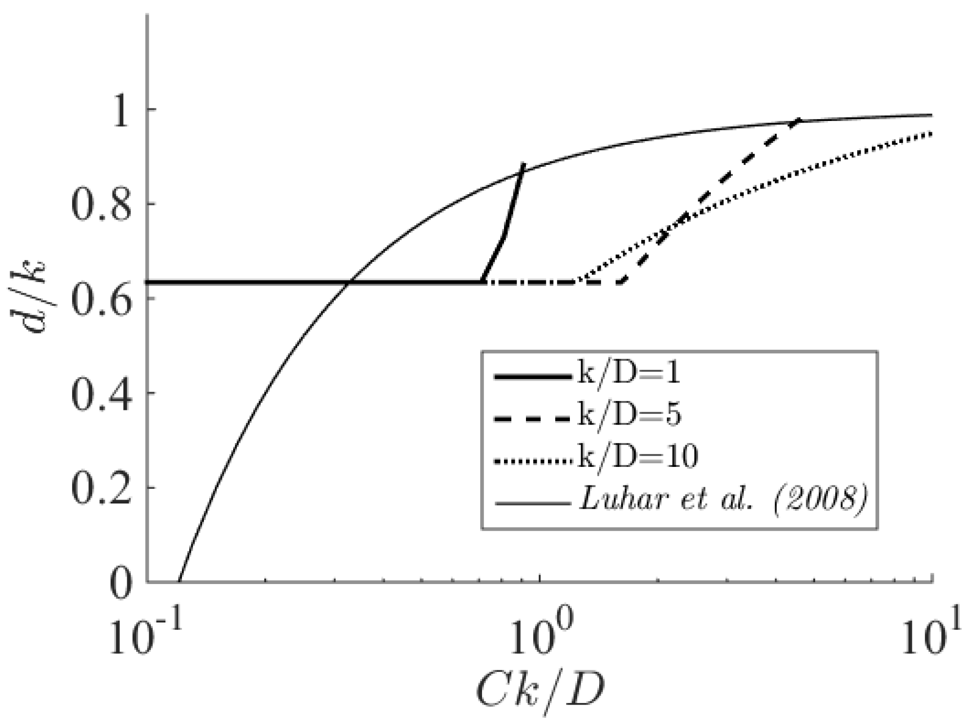
Figure 14.
Hydraulic roughness as a function of the confinement around a rough bed case C = 0.4, = 1, = 0.3.
Figure 14.
Hydraulic roughness as a function of the confinement around a rough bed case C = 0.4, = 1, = 0.3.

Figure 15.
Hydraulic roughness as a function of the spatial density.
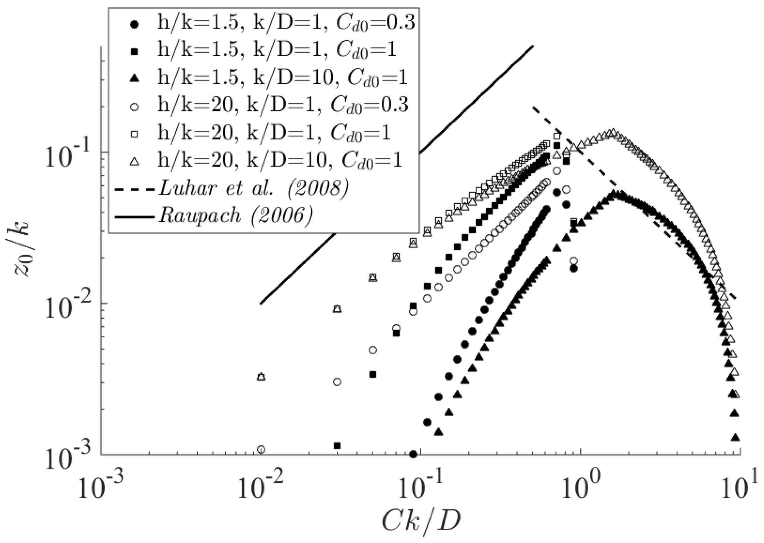
Figure 16.
Ratio between shear velocity and velocity at the top of the canopy as a function of the spatial density.
Figure 16.
Ratio between shear velocity and velocity at the top of the canopy as a function of the spatial density.

Figure 17.
Friction coefficient as a function of the geometrical model parameters ( = 0.3, = 0.5, C = 0.4 for the parameters which do not change).
Figure 17.
Friction coefficient as a function of the geometrical model parameters ( = 0.3, = 0.5, C = 0.4 for the parameters which do not change).


Table 1.
Dimension of macro-roughness. Data from [23] are corrected with the shape factor considering that the short axis is the dimension facing the flow D.
Table 1.
Dimension of macro-roughness. Data from [23] are corrected with the shape factor considering that the short axis is the dimension facing the flow D.
| D (mm) | k (mm) | C | Shape | |
|---|---|---|---|---|
| [17] | 35 | 30–100 | 0.08–0.2 | cylinder |
| [24] | 20 | 7 | 0.41 | truncated cone |
| [1] | 38 | 19 | 0–0.38 | hemisphere |
| [20] | 20 | 10 | 0.078/0.14/0.30 | hemisphere |
| [18] | 38–76 | 26–57 | 0–0.9 | pebbles |
| [21] | 3.2–8.3 | 100 | 0.05–0.15 | cylinder |
| [22] | 46–108 | 23–54 | 0.06–0.82 | hemisphere |
| [23] | (25.4–38.1) | (25.4–38.1) | 0.04–0.8 | gravels |
| [23] | (127–250) | (127–250) | 0.09–0.83 | cobbles |
| [19] | (620–830) | (220–410) | 0.05–0.37 | rocks |
Table 2.
Hydraulic conditions and experimental correlation for rock ramp resistance.
| h/k | S(%) | C | ||
|---|---|---|---|---|
| [7] | 0.4–2 | 2.5–22 | rock ramp | |
| [5] | 0.5–6 | 0.5–3 | rock ramp | |
| [1] | 1–4 | 2.4–8.8 | 0–0.38 | |
| [25] | 0.1-30 | / | various |
Table 3.
Models used to compute vertical velocity profile in the case of submerged roughness [14]: d is the displacement in the logarithmic law, is the hydraulic roughness, is a turbulence length scale between the macro-roughnesses, and the von Kármán constant (=0.41). The expression of these parameters results from the continuity of velocity and its gradient at the top of the roughness elements.
| u (m s) | Parameters | |
|---|---|---|
| Upper layer | ||
| Lower layer | ||
| = |
© 2017 by the authors. Licensee MDPI, Basel, Switzerland. This article is an open access article distributed under the terms and conditions of the Creative Commons Attribution (CC BY) license (http://creativecommons.org/licenses/by/4.0/).
Share and Cite
MDPI and ACS Style
Cassan, L.; Roux, H.; Garambois, P.-A. A Semi-Analytical Model for the Hydraulic Resistance Due to Macro-Roughnesses of Varying Shapes and Densities. Water 2017, 9, 637. https://doi.org/10.3390/w9090637
AMA Style
Cassan L, Roux H, Garambois P-A. A Semi-Analytical Model for the Hydraulic Resistance Due to Macro-Roughnesses of Varying Shapes and Densities. Water. 2017; 9(9):637. https://doi.org/10.3390/w9090637
Chicago/Turabian StyleCassan, Ludovic, Hélène Roux, and Pierre-André Garambois. 2017. "A Semi-Analytical Model for the Hydraulic Resistance Due to Macro-Roughnesses of Varying Shapes and Densities" Water 9, no. 9: 637. https://doi.org/10.3390/w9090637
Note that from the first issue of 2016, this journal uses article numbers instead of page numbers. See further details here.