Geometry Defeaturing Effects in CFD Model-Based Assessment of an Open-Channel-Type UV Wastewater Disinfection System


1
Department of Mechanical Engineering, Hanyang University, 222 Wangsimni-ro, Seongdong-gu, Seoul 04763, Korea
2
Research laboratory, Ecoset Co., Ltd., 15 Emtibeui 1-ro, Danwon-gu, Ansan-si 15610, Korea
*
Author to whom correspondence should be addressed.
Water 2017, 9(9), 641; https://doi.org/10.3390/w9090641
Submission received: 25 July 2017
/
Revised: 13 August 2017
/
Accepted: 25 August 2017
/
Published: 27 August 2017
Abstract
:Computational fluid dynamics (CFD) is a popular tool in the water industry for assessing ultraviolet (UV) reactor performance. However, due to the size of open-channel-type UV reactor systems, the CFD model requires significant computational time. Thus, most evaluations have been conducted using very simplified models. In order to ensure the reliability of this simplified CFD model, precise numerical modeling and validation by measurements are necessary considering the geometry defeaturing level. Therefore, simplified geometries in four defeatured levels were prepared for the CFD model, and simulations were performed to determine the level of geometric simplicity required to derive reliable results. A bioassay test was also conducted for a pilot-scale open-channel-type UV reactor that has the same geometrical configuration as the CFD model. Good agreement was observed between the bioassay test and CFD model results. It was found that the reduction equivalent dose (RED) is not significantly affected by geometry defeaturing under the assumption that the inlet flow conditions are relatively uniform. In multiple bank operation, the addition of banks yields a linear increment of the RED in the CFD model, however, a lower RED than the measured value was presented, especially for serial bank addition. The related aspects of the detailed flow physics and disinfection characteristics were also presented. These results are expected to provide useful information for CFD modeling, reactor design, and the assessment of the open-channel-type UV reactors.
1. Introduction
Disinfection is one of the most important issues in water treatment because it is directly related to public health and the ecosystem. Applications of ultraviolet (UV) light for this purpose have been used extensively for drinking and waste-water plants. UV disinfection is an eco-friendly technology without hazardous by-products that are produced by chemical disinfection methods such as chlorination [1]. For waste-water disinfection, open-channel type UV reactor systems are widely employed for final water treatment. The proper assessment of the UV reactor system is a key parameter that affects both the cost and reliable disinfection performance in given operating conditions. However, assessing these UV reactors is somewhat complex. The water flow, UV radiation intensity, and the reaction kinetics should be taken into account. Moreover, unlike close-conduit UV reactors, open-channel UV reactors have a free surface flow that further complicates the hydraulic behavior and its analysis. In the UV reactor, spatial differences in the UV radiation field and the differences in the residence time of water elements cause a certain distribution of the UV dose (hereinafter referred to as dose), which is defined as the amount of UV light exposed to microorganisms in the water elements. From these dose distributions, the reduction equivalent dose (RED) is calculated as the disinfection performance, and the size of the UV reactor is determined for target applications.
The disinfection performance is usually evaluated using experimental techniques such as biological dosimetry [2], Lagrangian actinometry [3,4], and optical diagnostic techniques [5,6]. Experimental methods are advantageous in that they can obtain accurate data without uncertainties related to the UV reactor design. However, they are disadvantageous in that the costs associated with testing different configurations and modifying the design are high. By contrast, theoretical methods [7,8] enable engineers to quickly estimate the initial size of the UV system. However, theoretical methods are prone to failure when predicting the delivered dose because real-world factors, such as detailed hydraulic behavior, are not considered.
To overcome the disadvantages of these methods, numerical modeling based on computational fluid dynamics (CFD) tools has been extensively used to design and evaluate the disinfection performance of the UV reactors [9]. The CFD modeling of UV reactors has the advantage that the water flow and related aspects such as the transfer and mixing processes of pathogenic microorganisms can be calculated at relatively low costs and with different testing configurations for initial sizing, prototype design, and optimization. Moreover, unlike bioassay testing, the CFD model allows one to visualize the physical parameters and provides insight into the physical phenomena that occur inside a UV reactor.
However, due to the geometrical size and multiphase flow of the open-channel UV disinfection systems, the CFD model requires significant computation time (e.g., in this paper, it takes about two or three weeks to solve a flow condition using a modern workstation computer). In addition, in current industry, engineers frequently face numerous simulation cases within a short turnaround time. Consequently, most simulations have been performed using simplified models to reduce the computational cost, and reliability would be liable to loss. In order to ensure the reliability of the CFD results, precise numerical modeling and validation are necessary. Additionally, the effects of the geometry defeaturing level on the results should be well understood.
Over the past two decades, many researchers have conducted CFD modeling and validation in attempts to understand the disinfection characteristics [10,11,12,13,14,15,16]; however, most of these studies focused on close-conduit-type UV reactors. Research into open-channel-type UV reactors is still limited in the literature. In particular, no prior research investigating detailed three-dimensional CFD modeling and validation of open-channel-type UV reactors is available in literature. Thus, it would be highly beneficial for design and assessment of the UV systems if information were available about geometry defeaturing effects and numerical validation in CFD modeling.
The objective of this study is to determine the geometry defeaturing level necessary to derive reliable simulation results and to understand the effects of geometry defeaturing level in the CFD modeling of open-channel-type UV disinfection systems. A bioassay validation test was performed to verify the validity of CFD modeling, and the detailed flow physics and disinfection characteristics are presented.
2. Materials and Methods
2.1. Model
The reactor used in this study is a Neotec NOL-HM UV disinfection system (Neotec Co. Ltd., Ansan-si, Korea). This reactor was designed based on CFD analysis results, which were obtained in the same manner as described in this paper. The NOL-HM UV disinfection system is an open-channel-type UV reactor with two banks of horizontal lamps. The lamp orientation and water flow direction are in parallel, as shown in Figure 1. Each UV bank consists of two modules, with eight lamps per module, for a total of 16 lamps per bank and 32 lamps in the entire system. The lamps are low-pressure UV lamps with an input power rating of 320 Watt; these have nearly monochromatic light with a wavelength of 253.7 nm. The specifications of the NOL-HM UV system are listed in Table 1.
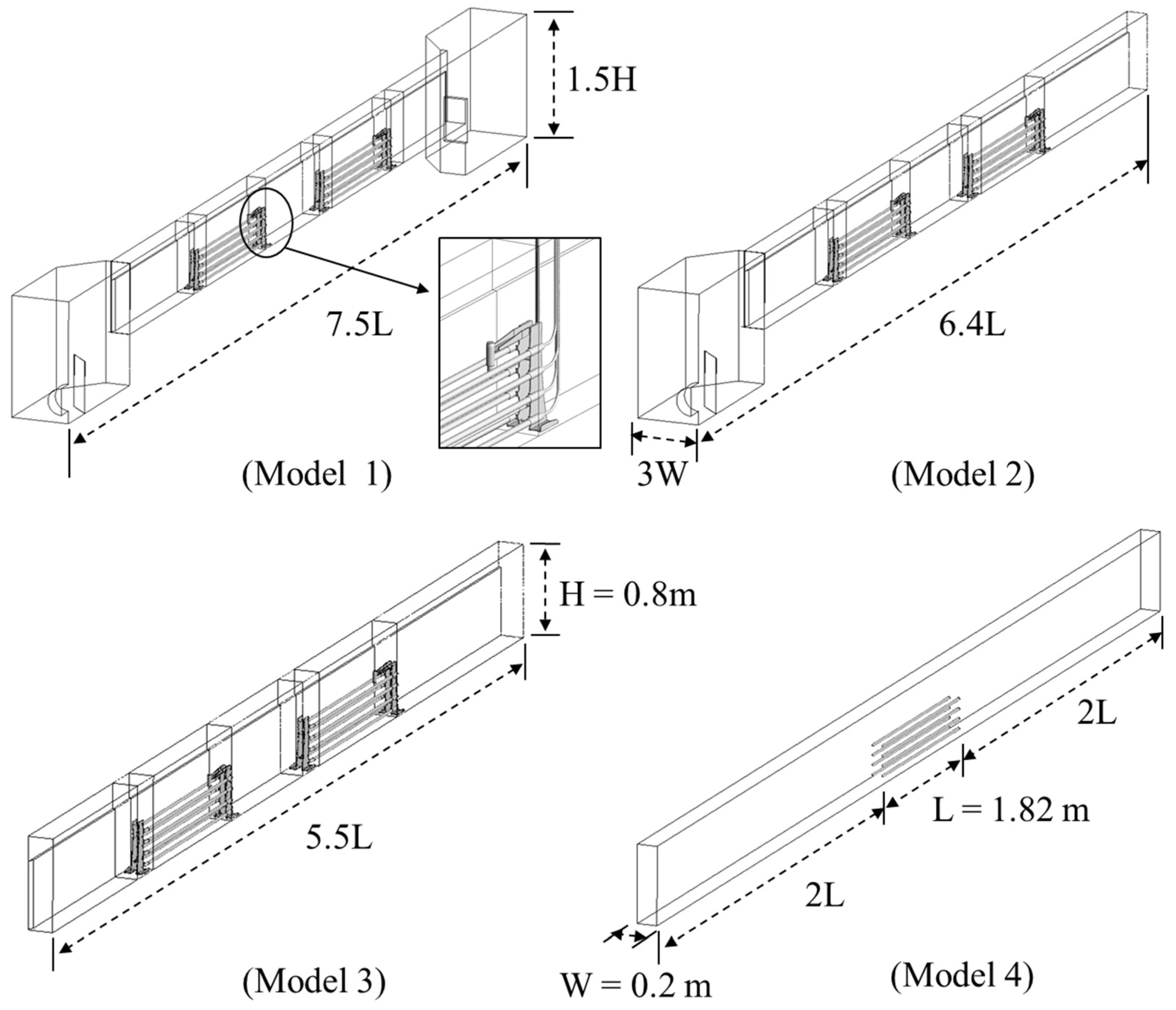
The total length and channel width of the pilot-scale UV reactor are 7.5 L and 2 W, respectively, where L is the length of the quartz sleeve, and W is half the width of the channel. To evaluate the bank addition and geometry defeaturing effect, four different geometries were generated as symmetrical models to reduce the computational cost. Simplification was performed on the assumption that the components in areas, where UV rays do not reach, do not affect the performance of the reactor. Model 1 (See Figure 1) is the same model as the pilot-scale UV reactor that was used in the bioassay test. A wiping system for cleaning the quartz tubes is not equipped in these experiments; hence, the wiping system was not modeled. Model 2 is the same model as Model 1; however, the electrical wires for supplying power to the lamp and water gate were neglected. Therefore, the water level is numerically calculated as function of density, gravity, and height. Model 3 is the same model as Model 2; however, the inflow reservoir and baffle plate were neglected. Therefore, the inflow velocity profile is relatively uniform upstream of the bank. Model 4 is a very simplified model. It has only a single lamp in the middle of the channel without any lamp supports. To reduce the computational cost and secure convergence, all models are generated as symmetrical models.
To maintain consistency between the experiments and the numerical model, geometry defeaturing and mesh generation were carefully performed, as shown in Figure 2. However, to decrease the number of elements and reduce the mesh generation efforts, a perforated plate was modeled with porous media and was located between the inflow reservoir and channel. The hybrid mesh was used for computation, the channel and lamp regions consist of multiblock-structured hexahedral elements, and the lamp support regions were composed of a tetrahedral-prism mesh. Non-conformal regions between the hexahedral and tetrahedral-prism mesh regions were numerically interfaced. The mesh-independent test was performed with various streamwise node densities at the lamp regions with reference to the literature by Saha [17]. Then, another component mesh, such as the lamp support and water gate, was created to maintain the quality of the mesh. The final mesh element counts are listed in Table 2.
2.2. Bioassay Test
A bioassay validation test was performed at the Fresno/Clovis Regional Wastewater Reclamation Facility in Fresno, California, USA. This test was performed as part of the Title 22 certification of California. Figure 3 shows a photo of the testing site and the pilot-scale NOL-HM UV disinfection system. The testing and data analysis were performed in accordance with the Ultraviolet Disinfection Guidelines for Drinking Water and Water Reuse [18] with Carollo Engineers Inc., (Walnut Creek, CA, USA) because Title 22 of the California Code of Regulation requires a third-party validation test.
The testing schematic is shown in Figure 4. Prior to the start of bioassay testing, hydraulic tests were conducted to determine the hydraulic residence time (HRT) and proper mixing of dosed constituents. Hydraulic testing was conducted by injecting SuperHumeTM (an organic humic acid concentrate that is used to reduce the UV transmittance (UVT) of water) into the piping upstream of the UV reactor. This test demonstrated that good mixing occurred at the given test point. After the lamp output and flow head became stable, bioassay testing was conducted by adding concentrated non-pathogenic indicator viruses, i.e., Escherichia coli bacteriophage MS2 (ATCC® 15597-B1™, Manassas, VA, USA), to the influent water. The MS2 phages were prepared with quality control, and all of the MS2 used during these tests met the quality control requirements established by UV Guidelines [18]. Samples were collected from the influent and effluent of the UV reactor to determine the inactivation of MS2 through the disinfection system for a range of flow rates and water UVTs at 254 nm. The mass flow rate (MFR) in the validation test ranged from 0.567 kg to 6.678 kg per second per lamp (kg s−1 lamp−1) at UVTs ranging from 52.7 to 75.9%. A total of 29 bioassay tests were conducted. Three influent and three effluent samples were collected for each test. The summarized experimental parameters can be found in the Supplementary Materials Tables S1 and S2, however, the detailed testing method and analysis are not discussed here, because this paper focuses on the CFD methodology and analysis.
2.3. Numerical Techniques
A commercially available CFD code, i.e., ANSYS CFX 14.5 (Ansys Inc., Canonsburg, PA, USA), was used to solve the flow in the open channel. Three phases were used to calculate the hydraulic flow fields: water, air, and solid particles that are equivalent to pathogenic organisms. However, the CFX does not support calculations for particle tracking consisting of two continuous fluids. Therefore, in this study, the air phase was calculated as a dispersed phase. The hydraulic flow field is determined by solving a system of steady-state 3D Reynolds Averaged Navier–Stokes (RANS) equations with the volume-weighted mixture density and viscosity. To calculate the water–air flow fields, a Eulerian–Eulerian homogeneous multiphase flow model was applied with an eddy-viscosity based k-ω SST turbulence model [19]. In the homogeneous multiphase flow model, the two fluids (water and air), share the same momentum and turbulence fields within the computational domain [20,21]. This assumption depends on the observations that the water–air interface (free surface) is distinctly defined in the channel, and that there is no entrainment of one fluid (air) into the other. Therefore, the finite-volume elements have flow properties corresponding to either air or water far from the free-surface. Alternatively, in elements that are close to containing the free-surface, the flow properties can be determined by mixtures of the phases depending on their volume fractions. In this study, the shape of the free surface was computed via water–air interface capturing based on a volume of fluid (VOF) method [21]. In the VOF approach, the free surface is captured by solving a continuity equation for the volume fraction of the heavier fluid, water (. Then, the volume faction of air can be calculated as . In given elements, the summation of the volume fraction of water and air should be unity. Therefore, the free surface is calculated by determining the elements where the volume fraction is .
Alternatively, the movement of microorganisms through the UV reactor was simulated by the Lagrangian particle tracking method because microorganisms (modeled as particles in CFD) are physically discrete in water. The trajectory of particle calculations uses information that is generated by the flow field simulation; that is, the individual particles in the computational domain are tracked by solving Newton’s second law for the forces acting on particles in a Lagrangian frame of reference. Although several different forces affect the motion of a particle in a fluid, only the viscous drag, buoyancy (gravity), and turbulent dispersion force were considered in this study. The other forces, such as pressure gradient forces and Brownian motion, are neglected.
All governing equations were discretized using an element-based finite-volume method [22]. For the discretization of convection terms, a high-resolution scheme [23] was applied. This scheme blends the first order upwind and the second-order upwind in order to reduce the numerical diffusion error. To determine the convergence for the flow field, the root mean square (RMS) residual and domain imbalances were used as convergence criteria. The water velocity at downstream of the lamp support of the second bank was monitored to assess the steady-state solutions. Converged solutions were obtained when the RMS residual was less than 1.0 × 10⁻⁵ for all independent variables in Model 3 and Model 4 (see Figure 1). However, in Model 1 and Model 2 (see Figure 1), converged RMS values were less than 1.0 × 10⁻⁴ due to the unsteadiness of the flow. Nevertheless, global imbalance in each domain for all simulation cases was less than 0.01% which indicates that conservation was achieved.
2.4. UV Radiation Model and Inactivation Kinetics
Although several UV radiation models have been proposed by various researchers, a model that can represent all of the radiation physics of an actual reactor has yet to be developed. Liu [24] experimentally compared the performance of several UV radiation models and showed that the effect of a quartz sleeve can easily and accurately be accounted for by using a correction factor for fluence rate (also known as UV intensity) predictions in the multiple-segment source summation (MSSS) model. The UVCalc3D software (v2013.09.03.100, Bolton Photosciences Inc., Edmonton, AB, Canada) that does not consider quartz sleeves but that does use a factor to account for the effects of quartz sleeves on the fluence rate distribution showed little difference with the results of the MSSS model [24]. Quartz sleeves were not considered in this work. Thus, the UVCalc3D software was selected based on its advantages of lower computational cost and reliable prediction performance. However, the UVCalc3D software is a stand-alone program; hence, a FORTRAN subroutine was created to integrate UVCalc3D’s UV data with the CFD code.
To obtain the delivered dose in the reactor, calculation procedure followed the method proposed by Ho et al. [25] and Wols et al. [26]. The UV irradiation field was integrated over each particle’s trajectory, as follows:
where represents the dose () that the amount of UV energy accumulated to each particle, and is the fluence rate at a specific finite volume element. The is the time taken to pass a specific finite volume. It can be calculated in two ways. One is to use the timestep of the solver, and the other is to get from the relationship particle displacement and particle velocity via post processing. Thus, calculation accuracy depends on the mesh size and UV radiation model. In this study, was calculated by UVCalc3D software, and was adopted from the solver value. Although Equation (1) is physically reasonable for calculating the cumulative dose in each particle track, some errors may be introduced due to the assumption mentioned in Section 2.4 and steady state simulation. However, according to the reported literature by Saha [16,17], it does not seem to affect the results.
The microbial inactivation of each particle can be calculated by dose–response curve which a function of the dose was fitted to a polynomial dose–response function using non-linear regression, as follows:
where represents the proportion of inactivated microorganisms at each particle track. The represents the dose () obtained from the collimated beam test or Equation (1). The kinetic parameters and were determined from the collimated beam test results. Averaging all of the particle tracks provides the total inactivation, as follows:
where represents the total number of particle tracks. From this total inactivation, the RED value for each simulation was calculated by solving the quadratic formula of Equation (2). On the other hand, the mean dose value obtained by averaging accumulated dose in each track, as follows:
Under ideal conditions, such as a collimated beam test, the RED and mean dose have the same value. However, since the velocity and fluence rate are not uniform in time and space, the two values are bound to differ.
2.5. Boundary Conditions
The boundary conditions used in the simulation are summarized in Table 3. For Model 1 (see Figure 1), the mass flow rate of water was specified at the inlet, and the opening condition of air was applied to the upper side of the channel. The outlet was considered to have atmospheric pressure conditions, and the other regions were specified to have no-slip wall conditions based on the logarithm wall-function. The outlets of Models 2–4 were set to have hydrostatic pressure as a function of water-level, density, and gravity (due to the lack of a water-gate). For Model 3 and Model 4, the inlet was set to have a mass flow rate with volume fraction that has a function of water-level; thus, Model 3 and Model 4 had uniform velocity profiles at inlet. For particle injection, a uniform concentration distribution is assumed at the inlet. Therefore, particles were uniformly released with zero-slip velocity conditions. That is, the velocity of particle is the same as the water velocity at a given point.
The properties of the particles, such as density and viscosity, were assumed to be the same as the properties of water because microorganisms consist of 70% or more water. Ducoste et al. [13] showed that the particle diameter is not critical for predicting the disinfection performance. Hence, the average particle diameter was set to be 1-μm, which is typical of most microorganisms found in wastewater. However, according to Munoz et al. [14], the number of particles does have an impact on the accuracy of the predicted dose distributions. To find the appropriate number of particles and maintain the statistical dose distribution, several tests were performed. In this study, an amount of 5000 particles was sufficient to obtain accurate results.
3. Results and Discussion
3.1. Collimated Beam Result
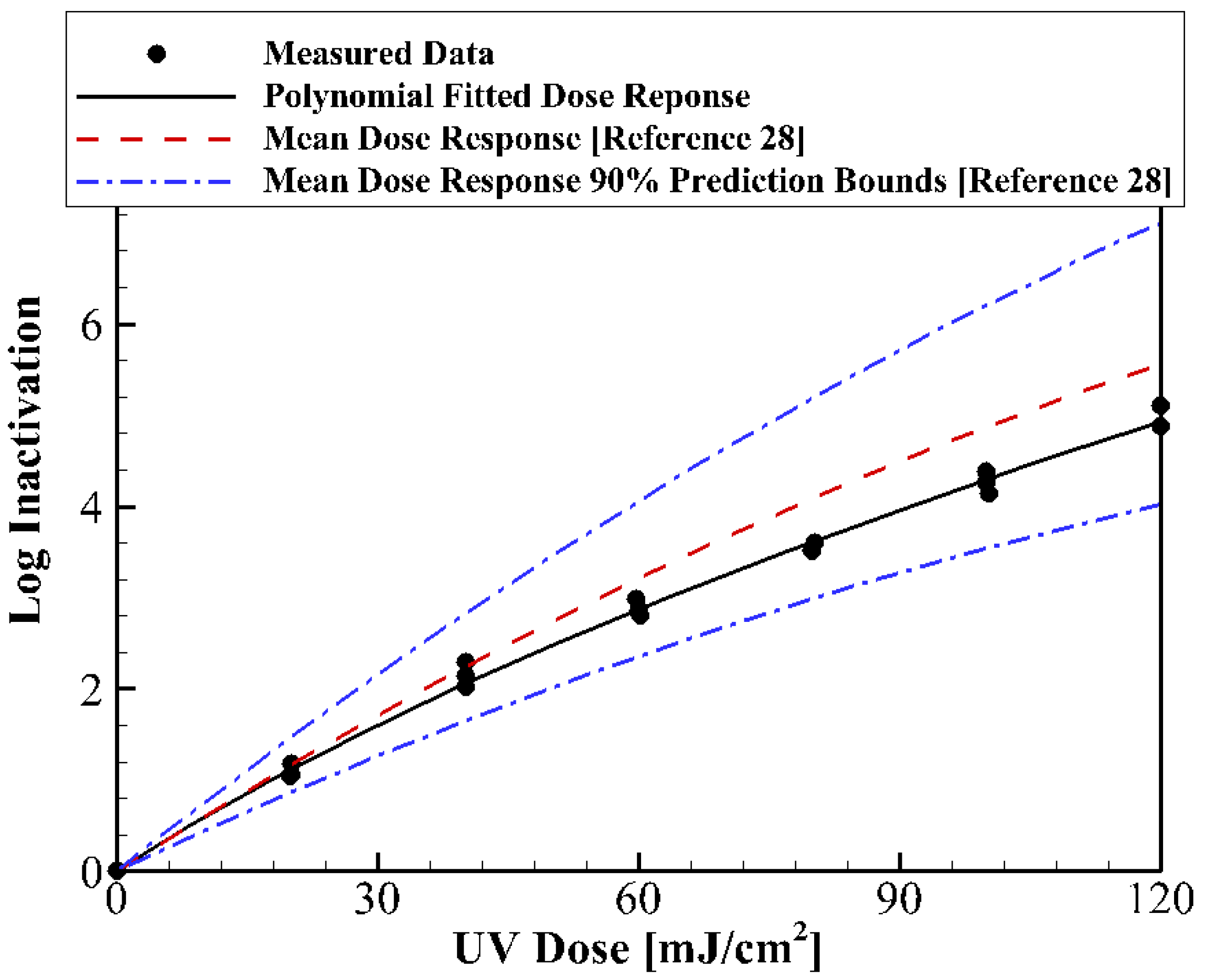
The inactivation of MS2 phages measured by the collimated beam apparatus was used to determine the dose–response curve of the phages, as shown in Figure 5. The observed inactivation response showed a somewhat lower log inactivation compared to the mean dose–response curve reported in literature [28]. However, the dose–responses lay within the 90% prediction interval of the mean response. The kinetic parameters of the polynomial-fitted dose–response curve (see Equation (2)) were calculated using the least-squares method; these were determined to be and . These parameter values were used to calculate the RED in the CFD results.
3.2. Validation of CFD Methods
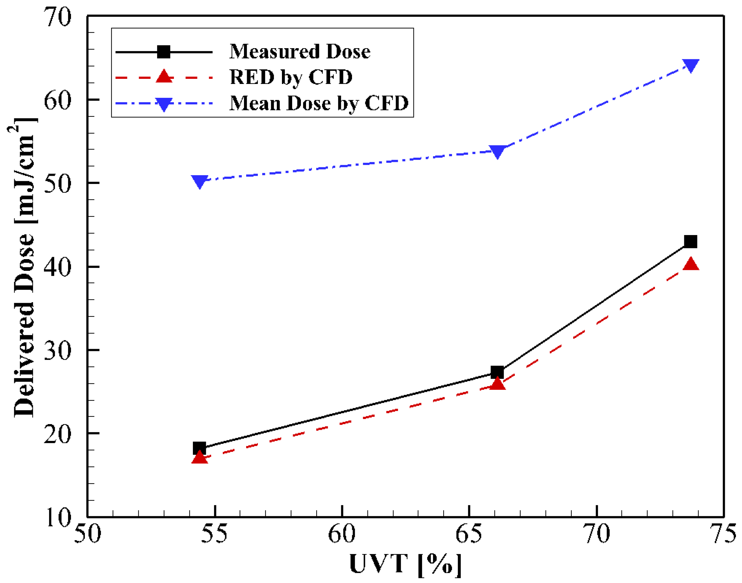
From the dose distributions determined by CFD modeling, the inactivation was predicted using the dose–response relations of the MS2 phages measured in the collimated beam tests. This allows a comparison between CFD modeling and bioassay tests for the pilot-scale UV disinfection system. The predicted RED values are plotted in Figure 6; the Measure Dose and RED by CFD represent the RED value by bioassay testing and CFD simulation, respectively. The mean dose can be calculated only through the CFD simulation, thus there is no value in the bioassay test. The results show good agreement between the CFD model and experimental results (within an error of 6%). Based on this, the CFD method utilized in this study can be used to reliably assess the disinfection performance in open-channel-type UV reactors with the RANS-based turbulence model and UVCalc3D.
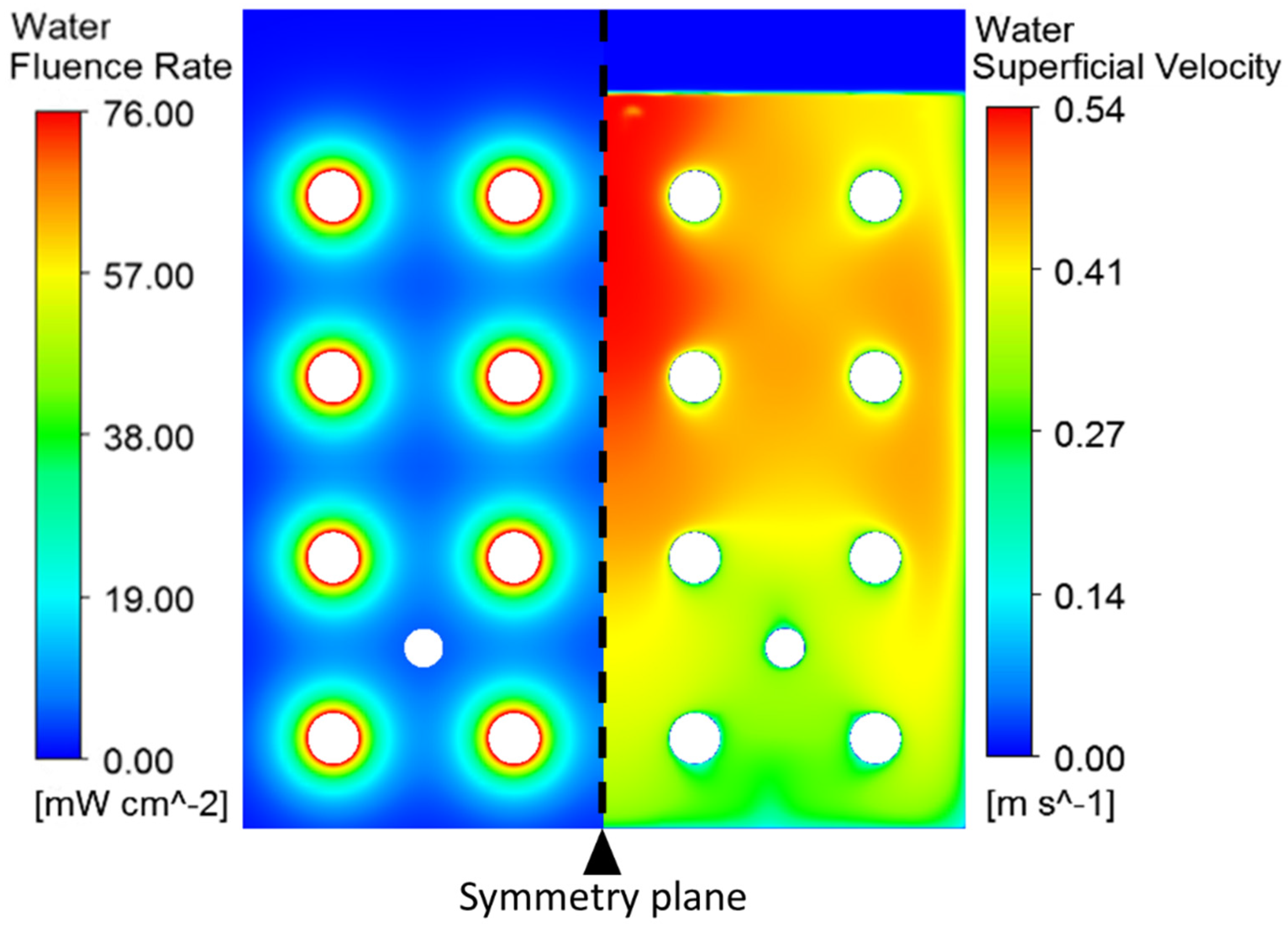
However, the differences between the mean doses obtained by the CFD model and the experimental results are relatively large and tend to decrease with decreasing the UVT (see Figure 6). The cause of these differences might be due to the non-uniform flow and spatial differences of the fluence rate distribution, as shown in Figure 7. The delivered doses in the UV reactor are related to the pathogenic microbes or viruses (modeled as particles in CFD), which moved in conjunction with the water flow between the quartzes sleeves of the UV lamps; where the water velocities are high and the fluence rate is relatively low. In addition, due to the boundary layer effects, the water velocities are very low closer to the quartz wall where the fluence rate is very high. Hence, particles are exposed to a higher fluence rate. Thus, the accumulative dose in each particle track at the reactor outlet is different.
The dose distribution determined from the particle’s accumulative dose at the reactor outlet is plotted in Figure 8. The frequency and cumulative represent the relative number of occurrence of the particle and its summation at the reactor outlet, respectively. The characteristics of the dose distributions can be clearly distinguished. The long tail in the dose distributions might be related to particles that move in the near-quartz and near-wall zones, which are low-velocity regions of the channel. At lower UVT and MFR, the peak value of the dose frequency curve is shifted toward lower doses. The peak is also higher and sharper due to the lower mean UV irradiance and higher mean residential time in the reactor. Alternatively, at higher UVT and MFR, the dose frequency becomes broader, which might be related to the higher degree of mixing of the water elements. Consequently, the difference between the RED and mean dose can be reduced, as shown in Figure 6. These tendencies are in accordance with those reported by Wols et al. [25].
3.3. Effects of Geometry Defeaturing
The delivered dose results for each model (see Figure 1) are shown in Figure 9 at a UVT of 73.7% and an MFR of 4.5 kg s−1 lamp−1 with power on one bank. Although Model 4 has a relatively simple configuration, the RED values of Model 1 and Model 4 are similar, with a difference around 6%. Additionally, the water gate (Model 2), inflow reservoir (Model 3), and lamp supports (Model 4) were also found to be not significant for RED prediction. To analyze these results, velocity contours and vectors at the center of first banks are plotted in Figure 10. The secondary flow patterns in Model 1 are stronger between the quartz sleeves of the lamps, whereas those in Model 4 are not. Generally, the secondary current contributes to the mixing of water elements, improves the disinfection performance, and increases the local velocity and velocity deviation.
However, an uneven velocity distribution at inflow does not seem to affect the mixing significantly; although Model 4 has a small secondary current (lower mixing) compared to Model 1, the RED value is similar to that of Model 1 due to the uniform flow of Model 4. In Figure 11, the frequency curve of Model 1 is moved slightly toward higher doses, and the peak abundance value is lower than that of Model 4. This resulted in an increment of the mean dose value and similar RED values, respectively. Thus, the amount of total UV energy is similar in both Model 1 and Model 4. Consequently, these models showed similar dose distributions at the reactor outlet, as presented in Figure 11. These results clarify the flow conditions at the inflow region of the banks. That is, if the velocity deviation is not large at the inflow region of the channel, mixing should be not necessary. Mixing devices such as the baffle typically involved head loss.
Even though the flow characteristics of Model 1 and Model 4 are different due to geometric defeaturing effects, from an engineering perspective and considering deviations in the reported data [28], this difference can be ignored in CFD modeling. This is because log inactivation of the MS2 phage can be varied between 1.65 and 2.82 at a dose of 40 , as shown in Figure 5. The differences in RED value caused by geometry defeaturing in the CFD model would be smaller than the uncertainty of the experimentally reported data.
Based on these results, simplified geometry can be used to calculate the performance of large-scale open-channel-type UV disinfection systems which are practically used in wastewater plants. This means that the number of mesh elements and simulation cost can be reduced. However, this assumption is only valid under relatively uniform inlet velocity conditions.
3.4. Effects of Bank Additions
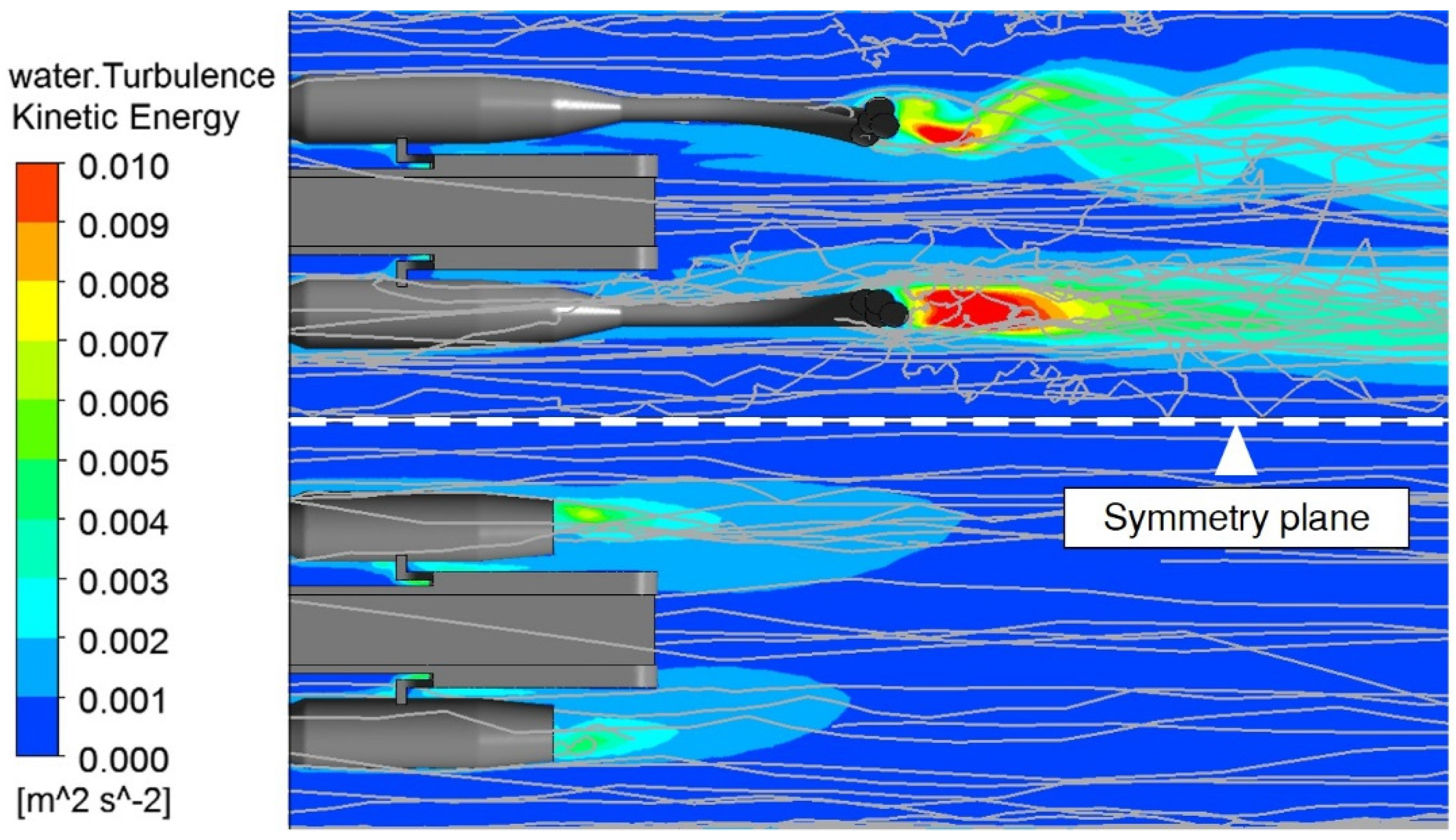
Full-scale UV disinfection systems used in wastewater plants typically consist of multiple UV banks arranged in series or parallels. The number of banks depends on the target log inactivation of pathogens, MFR, and head loss. The delivered doses from two banks operating in series are plotted in Figure 12 at a UVT of 54.4% with the same total mass flow. To analyze the effects of geometry defeaturing, the turbulence kinetic energy (TKE) and particle track are shown in Figure 13 (downstream of the first bank). Since the power line is ignored, the TKE of Model 2 is more quickly dissipated and the area is narrower than that of Model 1. However, it can be seen that the RED value does not change significantly in the presence of the power line. In the same way, it can be assumed that the lamp support will also not affect the RED prediction. Although the predicted RED and mean dose are almost doubled compared to those in the single-bank system (see Figure 12), the predicted RED values are lower than the measured dose. This indicates that the mixing cannot be fully captured in the series multi-bank CFD simulation with a symmetrical model. The mixing by, for example, vortex shedding may affect the disinfection performance as reported in the literature [29,30]. The full CFD model (not symmetrical model) involves oscillation of the water flow, which is generally observed in real channel flow [31], and convergence is impossible without unsteady simulation. Although unsteady simulation is becoming feasible due to advances in computational power, it remains justifiable only for special cases in the open-channel-type UV disinfection system. Even though the symmetrical 3D CFD model does not perfectly capture the flow physics of open-channel flow, it is still useful for assessing the disinfection performance.
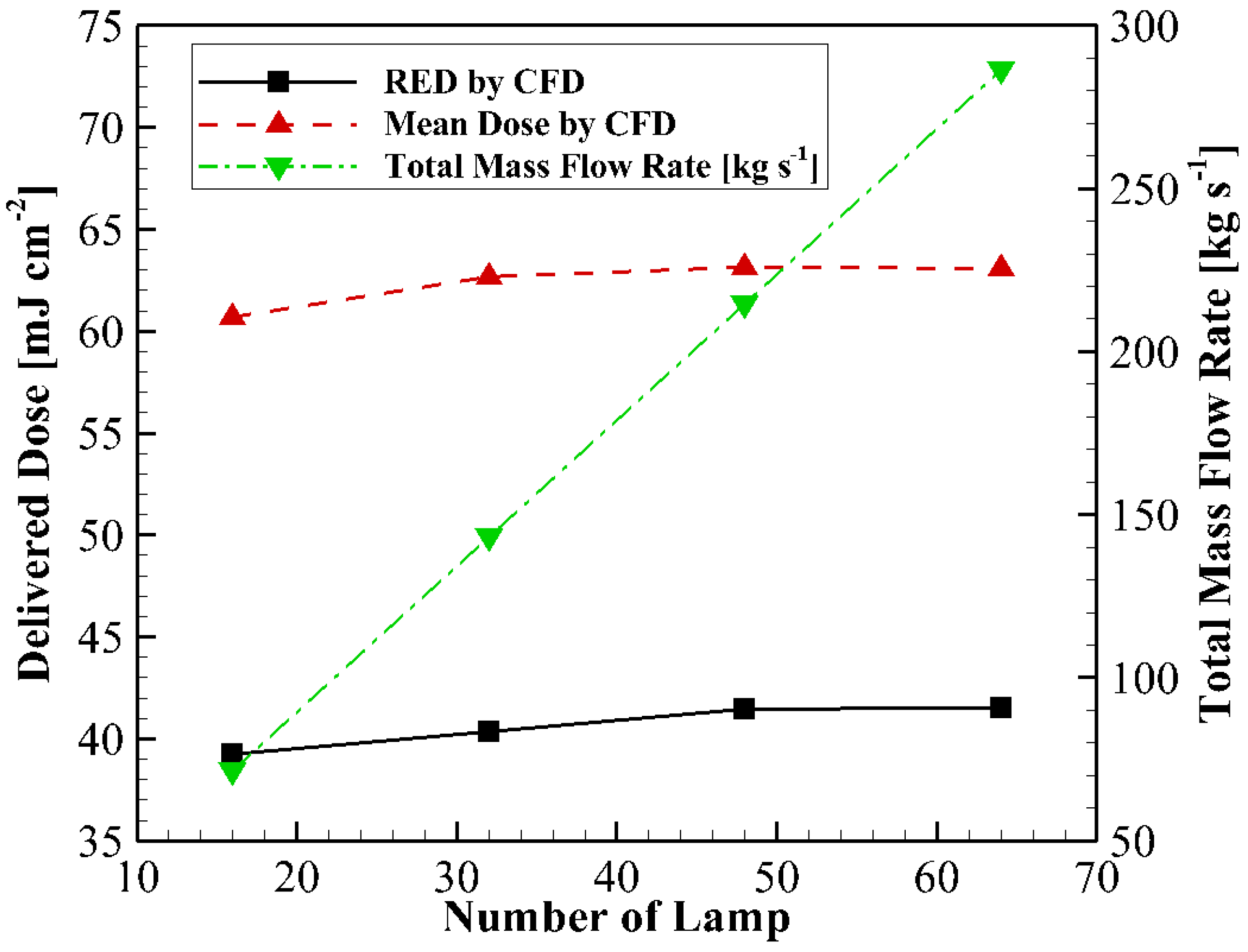
Alternatively, for multiple bank operation in parallel with Model 4, the difference in predicted RED value is only 4%, as shown in Figure 14. As the number of banks and MFR increase, the RED value becomes constant because the velocity becomes more uniform.
Among the above results, for the multiple bank simulation, it is found that the predicted RED in the CFD model is also not affected by the geometry defeaturing level; however, the actual delivered dose is significantly affected by mixing, which is not properly captured in the CFD model due to the limitations of the symmetrical model with steady simulation.
4. Conclusions
A CFD model and numerical techniques were established to assess the disinfection performance of an open-channel-type UV reactor. Good agreement was observed between the result of the bioassay test and CFD model when the same geometric configuration was used. To determine the geometry defeaturing effects in the CFD model for UV system design, four geometries were evaluated and compared with the bioassay test results. The findings from these studies lead to the following conclusions and recommendations:
- In CFD modeling, a simple geometry (only lamp and channel) configuration can be used to evaluate the disinfection performance of the full scale UV system, under the assumption that the inlet flow conditions are relatively uniform.
- For both site-specific operation or CFD modeling, if the inlet flow conditions are not severely distorted, flow mixing would not be necessary to ensure proper disinfection performance.
- In multiple bank operation, the addition of banks yields a linear increment in the RED of the CFD model, but the actual measured doses can be higher. Thus, the delivered UV doses predicted by the CFD model might be underestimated, especially for serial bank addition.
- One reason that may contribute to the discrepancy between the CFD model and measured doses is that mixing of the water by secondary current or oscillation characteristics in open-channel flow cannot be properly captured in steady-state simulation.
Supplementary Materials
The following are available online at www.mdpi.com/2073-4441/9/9/641/s1, Table S1: Equipment and parameter of bioassay testing, Table S2: Summary of bioassay test results.
Acknowledgments
This study is supported by Korea Environmental Industry and Technology Institute (KEITI, Grant No. 201600014001), Neotec Co., Ltd., and Ecoset Co., Ltd. The authors gratefully acknowledge approval of the publish to Ecoset Co., Ltd.
Author Contributions
Jeong-Gyu Bak conceived and developed the numerical simulation methods, and performed the numerical simulation, and analyzed the data under supervision of the Jinsoo Cho. Woochul Hwang designed the pilot scaled reactor and performed the experiments with Carollo Engineers, Inc.
Conflicts of Interest
The authors declare no conflict of interest.
References
- Oppenheimer, J.A.; Jacangelo, J.G.; Laine, J.-G.; Hoagland, J.E. Testing the equivalency of ultraviolet light and chlorine for disinfection of wastewater to reclamation standards. Water Environ. Res. 1997, 69, 14–24. [Google Scholar] [CrossRef]
- Cabaj, A.; Sommer, R. Measurement of ultraviolet radiation with biological dosimeters. Radiat. Prot. Dosim. 2000, 91, 139–142. [Google Scholar] [CrossRef]
- Bohrerova, Z.; Bohrer, G.; Mohanraj, S.; Ducoste, J.; Linden, K. Experimental measurements of fluence distribution in a UV reactor. Environ. Sci. Technol. 2005, 39, 8925–8930. [Google Scholar] [CrossRef] [PubMed]
- Blatchley, E., III; Shen, C.; Naunovic, Z.; Lin, L.; Lyn, D.; Robinson, J.; Ragheb, K.; Grégori, G.; Bergstrom, D.; Fang, S.; et al. Dyed Microspheres for Quantification of UV Dose Distributions: Photochemical Reactor Characterization by Lagrangian Actinometry. J. Environ. Eng. 2006, 132, 1390–1403. [Google Scholar] [CrossRef]
- Elyasi, S.; Taghipour, F. Performance evaluation of UV reactor using optical diagnostic techniques. AIChE J. 2011, 57, 208–217. [Google Scholar] [CrossRef]
- Gandhi, V.N.; Roberts, P.J.W.; Kim, J.H. Visualizing and quantifying dose distribution in a UV reactor using three-dimensional laser-induced fluorescence. Environ. Sci. Technol. 2012, 46, 13220–13226. [Google Scholar] [CrossRef] [PubMed]
- U.S. Environmental Protection Agency (EPA). Design Manual: Municipal Wastewater Disinfection; EPA Office of Research and Development: Washington, DC, USA, 1986.
- Lawryshyn, Y.; Hofmann, R. Theoretical Evaluation of UV Reactors in Series. J. Environ. Eng. 2015, 141, 04015023. [Google Scholar] [CrossRef]
- Zhang, J.; Tejada-Martínez, A.E.; Zhang, Q. Developments in computational fluid dynamics-based modeling for disinfection technologies over the last two decades: A review. Environ. Model. Softw. 2014, 58, 71–85. [Google Scholar] [CrossRef]
- Downey, D.; Giles, D.K.; Delwiche, M.J. Finite element analysis of particle and liquid flow through an ultraviolet reactor. Comput. Electron. Agric. 1998, 21, 81–105. [Google Scholar] [CrossRef]
- Lyn, D.; Chiu, K.; Blatchley, E.R., III. Numerical modeling of flow and disinfection in UV disinfection channels. J. Environ. Eng. 1999, 25, 17–26. [Google Scholar] [CrossRef]
- Liu, D.; Ducoste, J.J.; Jin, S.; Linden, K. Evaluation of alternative fluence rate distribution models. Aqua. J. Water Supply Res. Technol. 2004, 53, 391–408. [Google Scholar]
- Ducoste, J.; Liu, D.; Linden, K. Alternative Approaches to Modeling Fluence Distribution and Microbial Inactivation in Ultraviolet Reactors: Lagrangian versus Eulerian. J. Environ. Eng. 2005, 131, 1393–1403. [Google Scholar] [CrossRef]
- Munoz, A.; Craik, C.; Kresta, S. Computational fluid dynamics for predicting performance of ultraviolet disinfection—Sensitivity to particle tracking inputs. J. Environ. Eng. Sci. 2007, 6, 285–301. [Google Scholar] [CrossRef]
- Wols, B.A.; Hofman, J.A.M.H.; Beerendonk, E.F.; Uijttewaal, W.S.J.; van Dijk, J.C. A systematic approach for the design of UV reactors using computational fluid dynamics. AIChE J. 2011, 57, 193–207. [Google Scholar] [CrossRef]
- Saha, R.; Zhang, C.; Ray, M. Similitude in an Open-Channel UV Wastewater Disinfection Reactor. J. Environ. Eng. 2015, 141, 04014065. [Google Scholar] [CrossRef]
- Saha, R.K. Numerical Simulation of an Open Channel Ultraviolet Wastewater Disinfection Reactor. Master’s Thesis, The Univesity of Western Ontario, London, ON, Canada, 2003. [Google Scholar]
- National Water Research Institute (NWRI); American Waste Water Association Research Foundation (AWWARF). Ultraviolet Disinfection Guidelines for Drinking Water and Water Reuse, 3rd ed.; NWRI: Fountain Valley, CA, USA, 2012. [Google Scholar]
- Menter, F.R. Two-equation eddy-viscosity turbulence models for engineering applications. AIAA J. 1994, 32, 1598–1605. [Google Scholar] [CrossRef]
- Zwart, P.J. Numerical modeling of free surface and cavitating flows. In Proceedings of the Industrial Two-Phase Flow VKI Lecture Series, Brussels, Belgium, 23–27 May 2005. [Google Scholar]
- ANSYS. ANSYS CFX-Solver Theory Guide; ANSYS Inc.: Canonsburg, PA, USA, 2012. [Google Scholar]
- Schneider, G.E.; Raw, M.J. A skewed, positive influence coefficient upwinding procedure for control-volume-based finite-element convection-diffusion computation. Numer. Heat Transf. 1986, 9, 1–26. [Google Scholar] [CrossRef]
- Barth, T.J.; Jesperson, D.C. The design and application of upwind schemes on unstructured meshes. In Proceedings of the 27th Aerospace Sciences Meeting, Reno, NV, USA, 9–12 January 1989. [Google Scholar]
- Liu, D. Numerical Simulation of UV Disinfection Reactors: Impact of Fluence Rate Distribution and Turbulence Modeling. Ph.D. Thesis, North Carolina State University, Raleigh, NC, USA, 30 December 2004. [Google Scholar]
- Ho, C.K. Radiation dose modeling in Fluent. In Proceedings of the WEF Disinfection 2009 Workshop: Modeling UV Disinfection using CFD, Sandia National Laboratories, Albuquerque, NM, USA, 28 February 2009. [Google Scholar]
- Wols, B.A.; Hofman-Caris, C.H.M.; Harmsen, D.J.; Beerendonk, E.F.; van Dijk, J.C.; Chan, P.S.; Blatchley, E.R., III. Comparison of CFD, biodosimetry and Lagrangian actinometry to assess UV reactor performance. Ozone Sci. Eng. 2012, 34, 81–91. [Google Scholar] [CrossRef]
- Menter, F.R.; Ferreira, J.C.; Esch, T.; Konno, B. The SST Turbulence Model with Improved Wall Treatment for Heat Transfer Predictions in Gas Turbines. In Proceedings of the International Gas Turbine Congress, Tokyo, Japan, 2–7 November 2003. [Google Scholar]
- Pirnie, M.; Linden, K.G.; Malley, J.P.J. Ultraviolet Disinfection Guidance Manual for the Final Long Term 2 Enhanced Surface Water Treatment Rule; EPA office of Water: Washington, DC, USA, 2006.
- Younis, B.A.; Yang, T.H. Computational modeling of ultraviolet disinfection. Water Sci. Technol. 2010, 62, 1872–1880. [Google Scholar] [CrossRef] [PubMed]
- Younis, B.A.; Yang, T.H. Prediction of the effects of vortex shedding on UV disinfection efficiency. J. Water Supply Res. Technol. 2011, 60, 147–158. [Google Scholar] [CrossRef]
- Nezu, I. Open-channel flow turbulence and its research prospect in the 21st century. J. Hydraul. Eng. 2005, 131, 229–246. [Google Scholar] [CrossRef]
Figure 1.
The computational model for geometry defeaturing evaluation for an open-channel-type UV reactor. The lamp power line, water-gate, inflow-reservoir, and lamp supports are defeatured sequentially. Note that only symmetrical models are used for computational fluid dynamics (CFD) simulation in order to reduce the computational cost and convergence time.

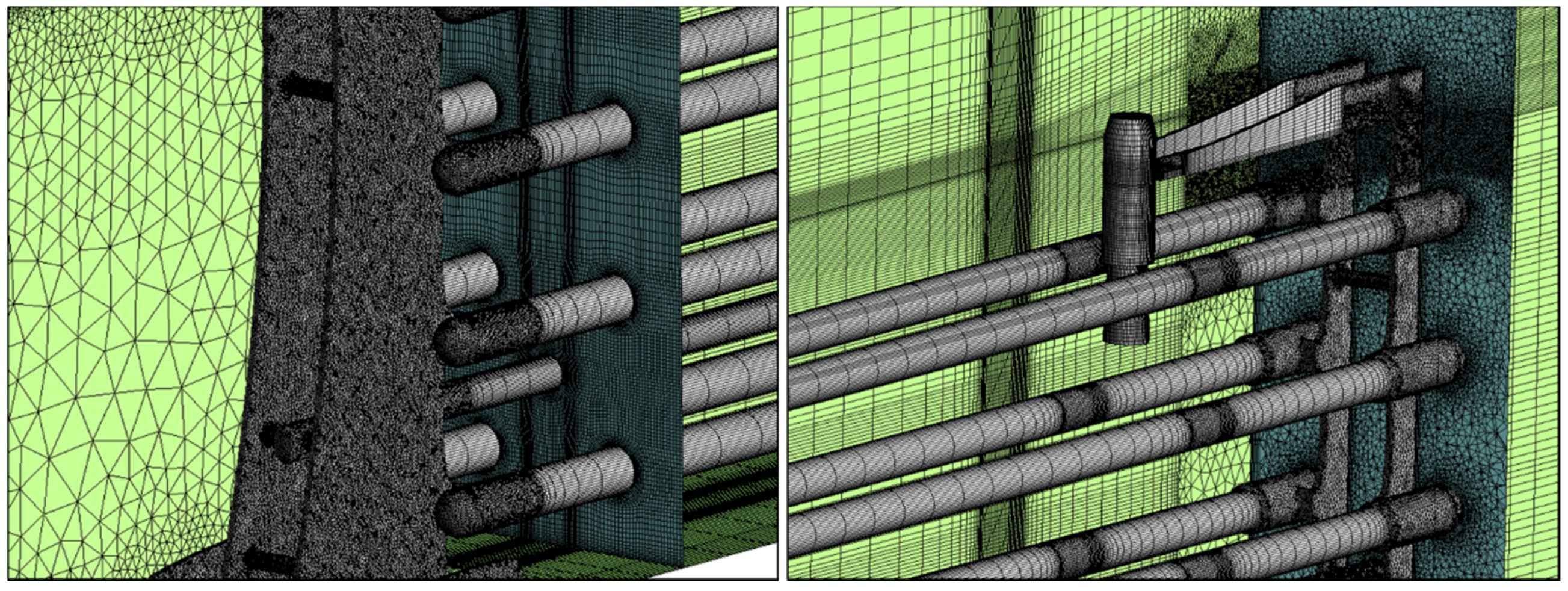
Figure 2.
Computational mesh for Model 2, showing the upstream side lamp support (left) and downstream side lamp support with UV sensor (right). To reduce the mesh generation effort and reduce number of elements, the lamp regions consists of multiblock-structured hexahedral elements.
Figure 2.
Computational mesh for Model 2, showing the upstream side lamp support (left) and downstream side lamp support with UV sensor (right). To reduce the mesh generation effort and reduce number of elements, the lamp regions consists of multiblock-structured hexahedral elements.

Figure 3.
Pilot-scale UV reactor at the testing site. The UV reactor contained 32 quartz sleeves aligned horizontal to the flow direction. UV lamps were installed in the quartz sleeves.
Figure 3.
Pilot-scale UV reactor at the testing site. The UV reactor contained 32 quartz sleeves aligned horizontal to the flow direction. UV lamps were installed in the quartz sleeves.
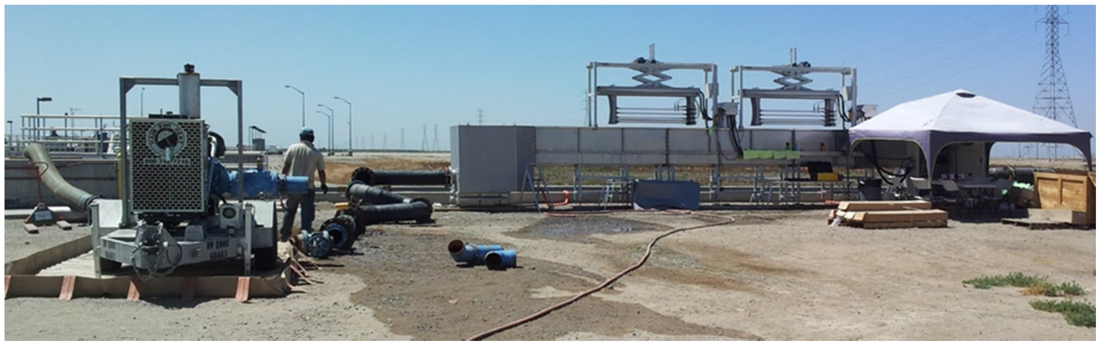
Figure 4.
Schematic of the bioassay test with the pilot-scale UV reactor.
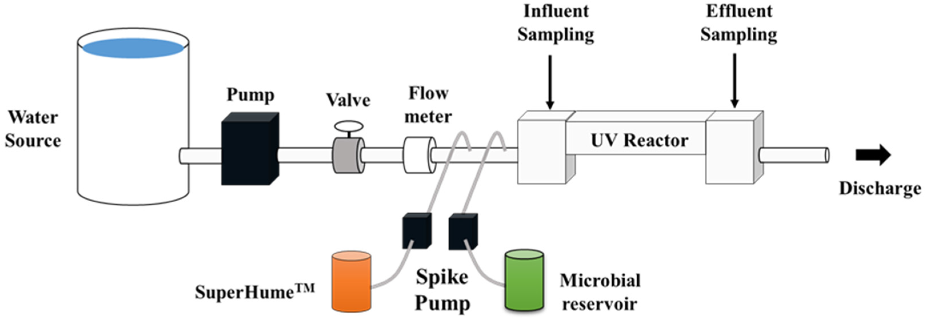
Figure 5.
Measured and polynomial-fitted dose–response curve of the MS2 phages. A quadratic UV dose–response equation is obtained as with .
Figure 5.
Measured and polynomial-fitted dose–response curve of the MS2 phages. A quadratic UV dose–response equation is obtained as with .

Figure 6.
Comparison between the bioassay test and CFD results for Model 1.

Figure 7.
Contours of the UV fluence rate (left) and velocity magnitude (right) at the middle of the first bank. (Simulation conditions: UV transmittance (UVT) = 66.1%, mass flow rate (MFR) per lamp = 3.91 kg s−1 lamp−1).
Figure 7.
Contours of the UV fluence rate (left) and velocity magnitude (right) at the middle of the first bank. (Simulation conditions: UV transmittance (UVT) = 66.1%, mass flow rate (MFR) per lamp = 3.91 kg s−1 lamp−1).

Figure 8.
Dose distributions calculated by CFD for the two experimental conditions.
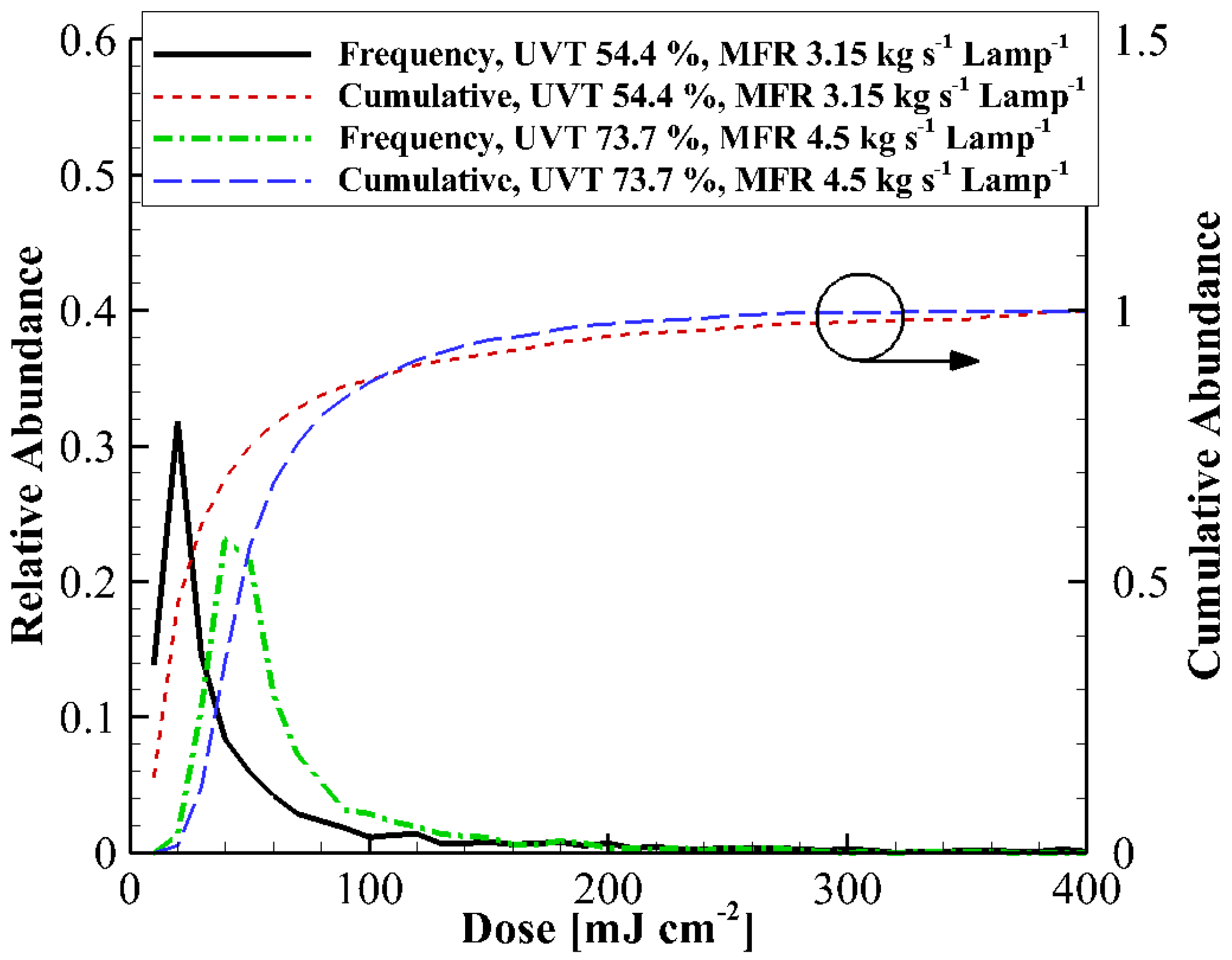
Figure 9.
Predicted delivered dose by CFD for the each CFD model at UVT = 73.7% and MFR per lamp = 4.5 kg s−1 lamp−1.
Figure 9.
Predicted delivered dose by CFD for the each CFD model at UVT = 73.7% and MFR per lamp = 4.5 kg s−1 lamp−1.
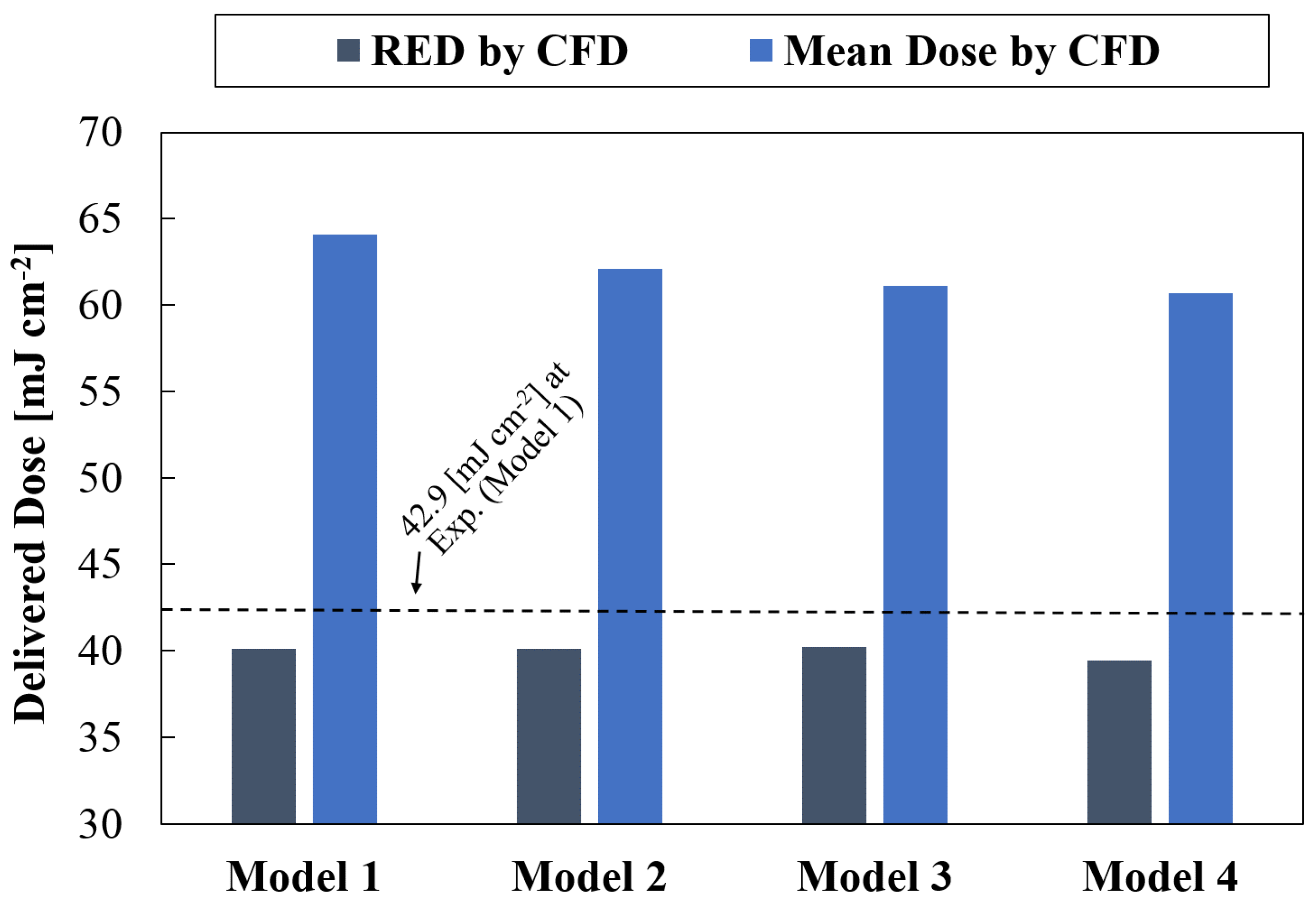
Figure 10.
Contours of the flow field (velocity in magnitude) and secondary-current velocity vector (tangentially projected to the plane) at the middle of the first bank for Model 1 (left) and Model 4 (right).
Figure 10.
Contours of the flow field (velocity in magnitude) and secondary-current velocity vector (tangentially projected to the plane) at the middle of the first bank for Model 1 (left) and Model 4 (right).
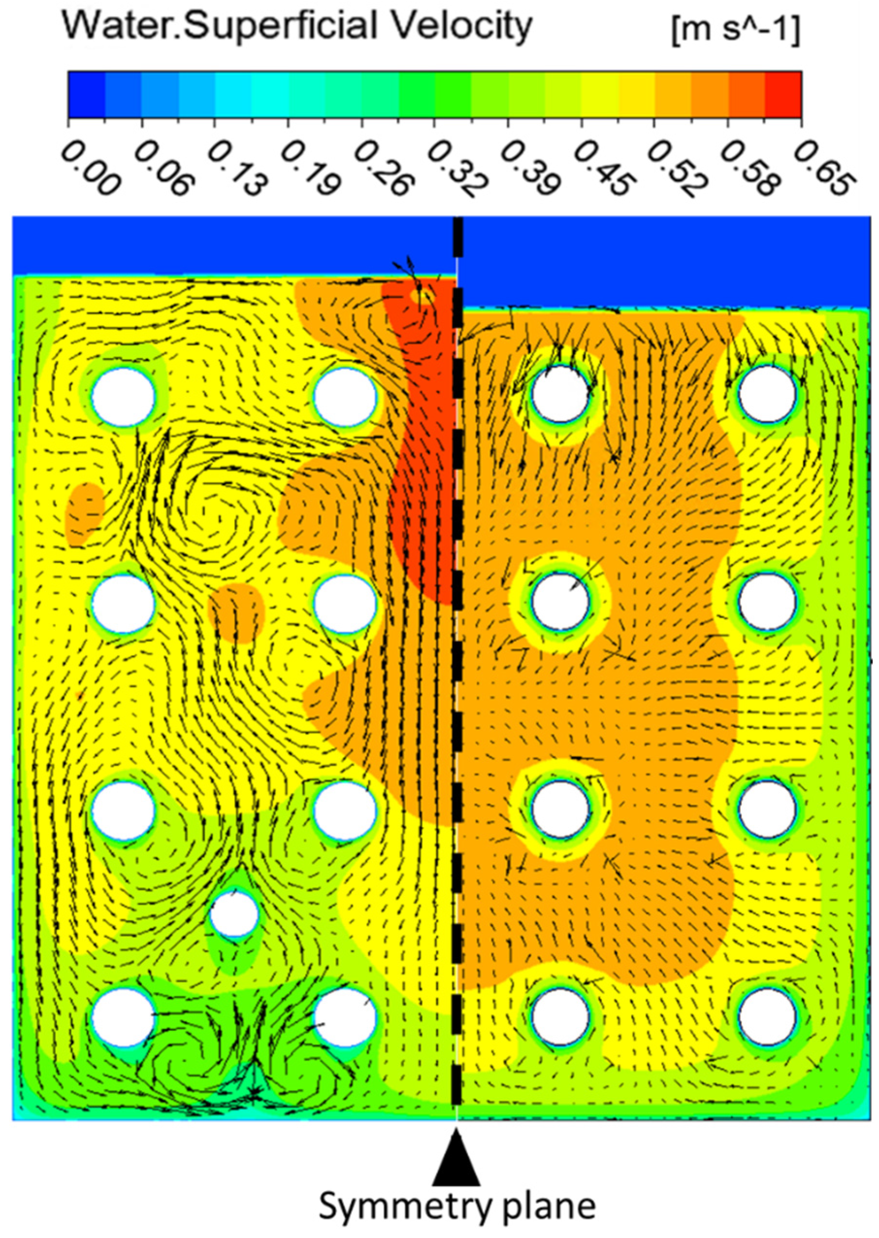
Figure 11.
Dose distribution computed by the CFD for the two CFD model at UVT = 73.7% and MFR per lamp = 4.5 kg s−1 lamp−1.
Figure 11.
Dose distribution computed by the CFD for the two CFD model at UVT = 73.7% and MFR per lamp = 4.5 kg s−1 lamp−1.
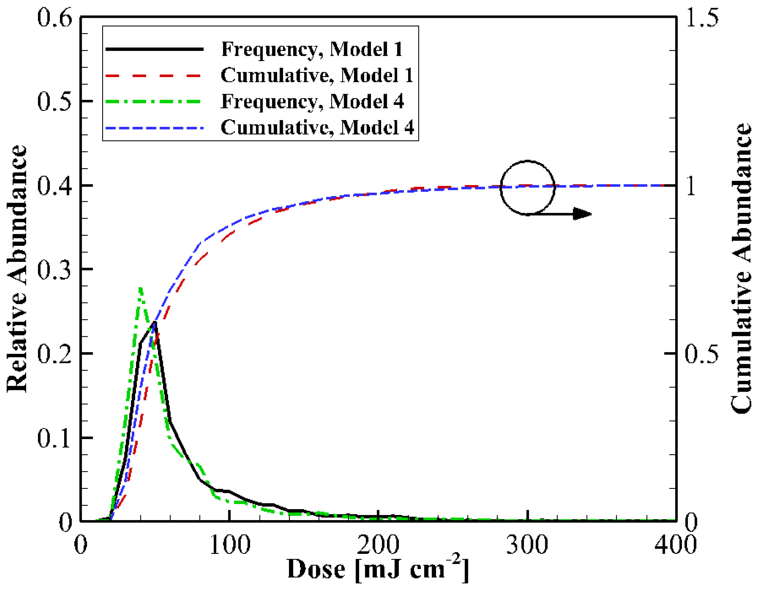
Figure 12.
Measured dose and predicted dose for serial bank addition at the UVT = 54.4% and total MFR = 25.2 kg s−1 in the channel.
Figure 12.
Measured dose and predicted dose for serial bank addition at the UVT = 54.4% and total MFR = 25.2 kg s−1 in the channel.

Figure 13.
Turbulence kinetic energy contours at the middle of the water level and particle tracks by the CFD model for Model 1 (upper) and model 2 (lower). The TKE of Model 2 is more quickly dissipated and particle tracks are smoother than those of Model 1.
Figure 13.
Turbulence kinetic energy contours at the middle of the water level and particle tracks by the CFD model for Model 1 (upper) and model 2 (lower). The TKE of Model 2 is more quickly dissipated and particle tracks are smoother than those of Model 1.

Figure 14.
Predicted dose for the parallel bank addition with Model 4 at the UVT = 73.7% and MFR per lamp = 4.5 kg s−1 lamp−1.
Figure 14.
Predicted dose for the parallel bank addition with Model 4 at the UVT = 73.7% and MFR per lamp = 4.5 kg s−1 lamp−1.

Table 1.
Specifications of the UV reactor for Title22 bioassay validation and CFD modeling.
| Parameters | Value |
|---|---|
| Reactor Type | Open channel |
| Sleeve Wiping System | None |
| Lamp Specification | Low-pressure amalgam lamp, maximum power of 320 W |
| Lamp Manufacturer | Light Sources, Inc. |
| Mounting Position of Lamp | Mounted horizontally and parallel to the flow |
| Number of Modules per Bank | 2 |
| Number of Lamps per Module | 8 |
| Total Number of Lamps per Bank | 16 |
| Number of Tested Banks per Reactor | 2 |
| Total Number of Lamps Tested | 32 |
| Operating Approach | “Dose-pacing” methodology |
Table 2.
Summary of the mesh counts for each model.
| Parameter | Model 1 | Model 2 | Model 3 | Model 4 |
|---|---|---|---|---|
| Elements 1 | 52.9 million | 39.9 million | 35.6 million | 6.2 million |
| Nodes | 22.3 million | 18.9 million | 14.4 million | 6.4 million |
1 The element counts are dramatically reduced with geometry defeaturing. The element count of Model 4 is less than the node counts due to the hexahedral element configuration.
Table 3.
Summary of the boundary conditions for each CFD model.
| Category | Model 1 | Model 2 | Model 3 | Model 4 |
|---|---|---|---|---|
| Inlet | Mass flow rate 1; VFw = 1, VFa = 0 | Mass flow rate; VFw = 1, VFa = 0 | Mass flow rate; is function of water level | Mass flow rate; is function of water level |
| Outlet | Pressure: 1 atm. | Hydrostatic pressure | Hydrostatic pressure | Hydrostatic pressure |
| Upper side | Opening: VFw = 0, VFa = 1 | |||
| Wall side | Automatic near-wall treatment [21,27] | |||
| Particle Injection | Number of Injection: 5000, Density: same as water, Diameter: 1-μm | |||
| UVCalc3D | Sleeve transmittance: 0.9, Sleeve R.I. 2: 1.51, Medium R.I.: 1.372 | |||
1 : Volume fraction of the water, : Volume fraction of the air, 2 R.I.: Refractive indices of medium.
© 2017 by the authors. Licensee MDPI, Basel, Switzerland. This article is an open access article distributed under the terms and conditions of the Creative Commons Attribution (CC BY) license (http://creativecommons.org/licenses/by/4.0/).
Share and Cite
MDPI and ACS Style
Bak, J.-G.; Hwang, W.; Cho, J. Geometry Defeaturing Effects in CFD Model-Based Assessment of an Open-Channel-Type UV Wastewater Disinfection System. Water 2017, 9, 641. https://doi.org/10.3390/w9090641
AMA Style
Bak J-G, Hwang W, Cho J. Geometry Defeaturing Effects in CFD Model-Based Assessment of an Open-Channel-Type UV Wastewater Disinfection System. Water. 2017; 9(9):641. https://doi.org/10.3390/w9090641
Chicago/Turabian StyleBak, Jeong-Gyu, Woochul Hwang, and Jinsoo Cho. 2017. "Geometry Defeaturing Effects in CFD Model-Based Assessment of an Open-Channel-Type UV Wastewater Disinfection System" Water 9, no. 9: 641. https://doi.org/10.3390/w9090641
Note that from the first issue of 2016, this journal uses article numbers instead of page numbers. See further details here.