Enhanced Two Dimensional Hydrodynamic and Water Quality Model (CE-QUAL-W2) for Simulating Mercury Transport and Cycling in Water Bodies

1
State Key Laboratory of Water Resources and Hydropower Engineering Science, Wuhan University, Wuhan 430072, China
2
LimnoTech, Environmental Laboratory, Engineer Research and Development Center, Davis, CA 95616, USA
3
China Institute of Water Resources and Hydropower Research, Beijing 100038, China
*
Author to whom correspondence should be addressed.
Water 2017, 9(9), 643; https://doi.org/10.3390/w9090643
Submission received: 21 July 2017
/
Revised: 15 August 2017
/
Accepted: 21 August 2017
/
Published: 28 August 2017
Abstract
:CE-QUAL-W2 (W2) is a widely-used two-dimensional, laterally averaged, longitudinal/vertical, hydrodynamic and water quality model. This model was modified and enhanced to include a mercury (Hg) simulation module for simulating Hg transport and cycling in water bodies. The Hg simulation module in W2 is able to model the physical and biochemical processes including adsorption and desorption of Hg species on multi-solids, settling and resuspension, sediment burial of adsorbed Hg, diffusive exchange between water column and sediment layer, volatilization, and biogeochemical transformations among Hg species. This paper describes the Hg simulation module, W2 model validation and its application to the Xiaxi River, China, a historical Hg contaminated water body. The W2 model was evaluated using the Xiaxi River data collected in 2007 and 2008. Model results show that W2 was able to predict the total Hg and methylmercury concentrations observed for the Xiaxi River. The Xiaxi River W2 model also provides a foundation for the future investigations of Hg contamination in the Xiaxi River. This application demonstrated the W2 model capability in predicting complex transport and cycling of Hg species in water bodies.
1. Introduction
CE-QUAL-W2 (W2) is a two-dimensional (2D), laterally averaged, longitudinal/vertical, hydrodynamic and water quality model for simulating surface water bodies. Lateral averaging assumes lateral variations in velocities, temperatures, and constituents are negligible. This model has been continuously developed and maintained by the U.S. Army Corps of Engineers (USACE) and Portland State University since late 80s [1,2]. Since its first release in 1986, the W2 model has been successfully applied to hundreds of rivers, lakes, reservoirs and estuaries throughout the world for thermal and water quality investigations [3,4,5,6,7,8]. U.S. governmental agencies including USACE, U.S. Bureau of Reclamation (USBR), U.S. Geological Survey (USGS), U.S. Environmental Protection Agency (USEPA), and Tennessee Valley Authority (TVA) as well as numerous states, county, and local agencies have used this model as a management tool to evaluate the impacts of point and nonpoint pollution sources including organic wastes, nutrients, and temperature in water bodies. The W2 model has also been applied in China [6]. Cole and Wells [2] presented the model theory, fundamental equations, and application guidelines. The model complexity has increased significantly with the increasing complexity of water quality and management issues since its release. The latest version of the W2 model can simulate the complete eutrophication process in water bodies, including carbon, nitrogen and phosphorous cycles, multiple algae, epiphyte and macrophyte species, dissolved oxygen, etc. Additionally, a benthic sediment diagenesis module was integrated into the model to compute the sediment-water exchange fluxes of nutrients and sediment oxygen demand [9].
Mercury (Hg) is a global, persistent, and bioaccumulative toxic contaminant. Its organic form, methylmercury (MeHg), is the most biologically active and toxic form of Hg. It can accumulate in organisms within the food chain, such as fish, posing a risk to wildlife and humans [10,11,12]. Several models have been developed to simulate the transport and fate of Hg in aquatic environments. These models include the MCM [13], MERC4 [14], SERAFM [15], and WASP [16,17]. Although W2 is a powerful tool and can simulate up to 32 water quality constituents, the current W2 model does not have capability of simulating Hg transport and cycling in water bodies.
To effectively evaluate both the potential for harmful bioaccumulation and proposed measures to mitigate that harm, the spatial and temporal distribution of Hg within a water body should be characterized as completely as possible. There has been a need to bring the W2 to the state-of-art and adding Hg modeling capability. In this study, a Hg simulation module was developed and incorporated into the W2 model. With this enhancement, W2 model can directly simulate the transport and cycling of three Hg species in water bodies. After a series of model testing and validation studies, the enhanced W2 model was applied to the Xiaxi River for further evaluation of the model performance. The Xiaxi River, which drains the Hg mining area in Wanshan County, has been contaminated by numerous Hg tailings. Wanshan County, located in Guizhou Province, south-western China, was identified as a heavy Hg contamination site. The largest conglomeration of Hg mines and refining plants in China is located in this area [18]. Enhanced W2 model with a newly developed Hg simulation module was applied to the Xiaxi River. Besides evaluating the W2 performance, model results of this application were intended to provide insight into the long-term fate of MeHg and Total Hg (THg) along the river and the relative importance of different processes in Hg cycling. This application can also be used as a management tool to quantify the sources of Hg contamination, the distribution of Hg, the influence of changing environmental conditions, and long-term mitigation of Hg contamination within the watershed.
2. Hg Simulation Module within CE-QUAL-W2
One of the major concerns of Hg and its impact on the environments is its transformation to MeHg. Speciation plays a major role in determining the bioavailability of Hg species for MeHg transformation and toxicity of Hg to living organisms. Speciation also influences transport of Hg within and between environmental media [19,20,21,22]. Hg0 and HgII are the major chemical forms of Hg input into the environment from anthropogenic or natural sources [20]. During the biogeochemical cycling of Hg, MeHg can be produced. Hg biogeochemical cycle involves three species and multi-phases in nature. The Hg simulation module in the W2 model was designed to simulate three primary Hg species of environmental concern: Hg0, HgII, and MeHg. Hg0 is assumed to exist in the dissolved phase and only in the water column. HgII and MeHg are simulated for the water column and sediment layer. The three Hg species and their kinetic equations implemented in the Hg simulation module are described in detail in Zhang and Johnson [23], and briefly summarized here.
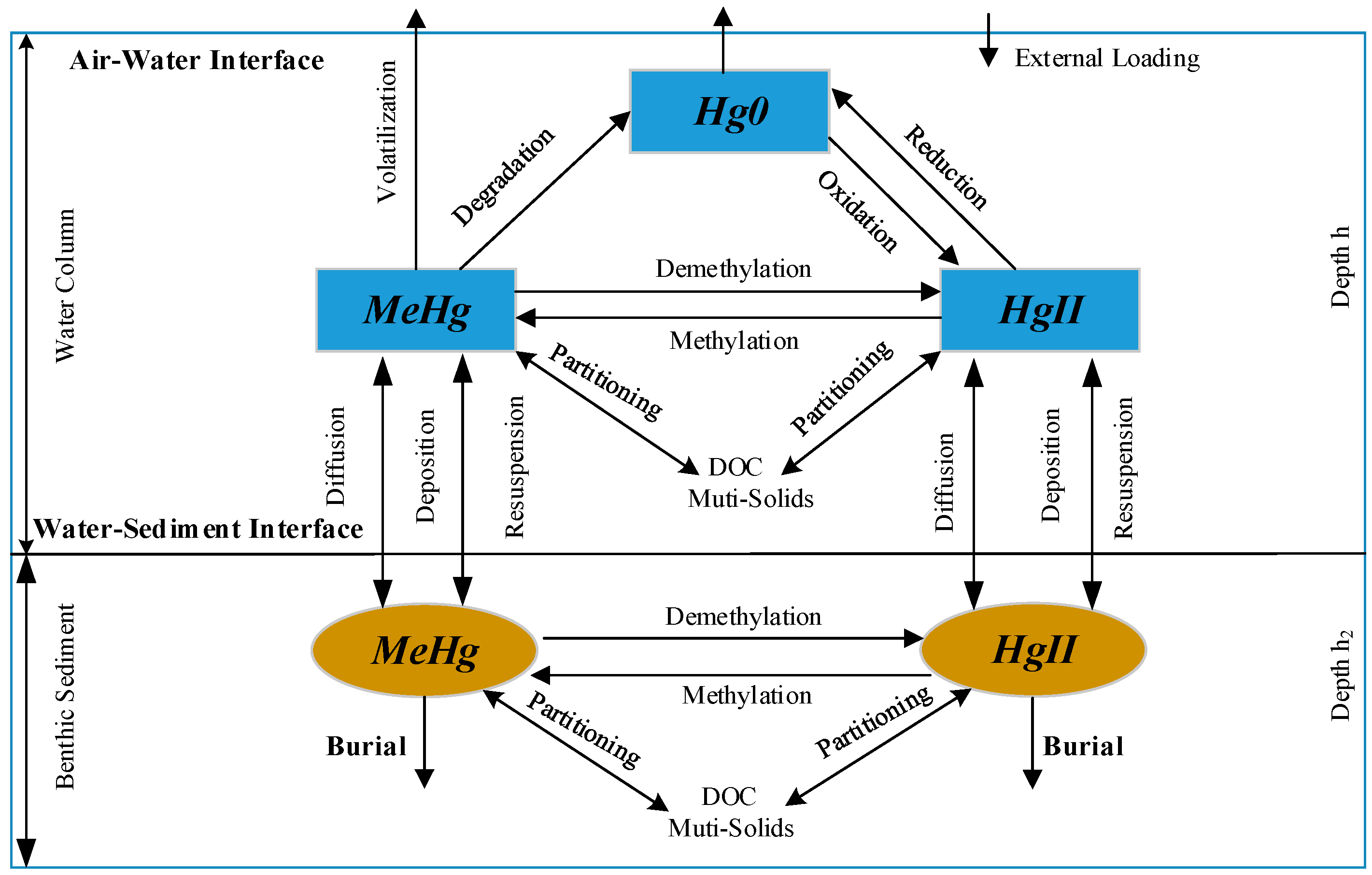
Hg0 is slightly water soluble and has a high Henry’s Law constant [24]. Hg0 constitutes very little of the total mercury in the surface water but may provide a significant pathway for the volatilization of Hg from surface waters. In the Hg simulation module, Hg0 is assumed to exist in the dissolved phase and only in the water column. MeHg and HgII exist in both the water column and the sediment layer and may distribute in dissolved phase and sorbed with dissolved organic carbon (DOC), particulate organic matter (POM), and inorganic solids. Physical and biochemical rate processes simulated in the Hg simulation module include: (1) adsorption and desorption of Hg species; (2) volatilization; (3) atmospheric deposition; (4) diffusive exchange between the water column and sediment layer; (5) deposition and re-suspension; (6) sediment burial of adsorbed Hg; (7) biogeochemical transformations among the three species. Figure 1 provides an overview of the model representation of the Hg species and their processes. Table 1 lists the symbols and definitions of concentrations of Hg species computed in the Hg simulation module.
The sediment layer represents the upper mixed layer and may be on the order of several centimeters thick due to bioturbation and mixing. Suspended sediments, with Hg bound to them, are deposited to and eroded from the sediment bed. Depending upon ambient concentrations of Hg species, the suspended sediments lost or gained to the water column become a source or sink for Hg. Once deposited, sediments coalesce to form an unconsolidated layer of variable, but often shallow depth. This active layer of sediments may undergo continual bioturbation, or mixing by organisms, so that sediments and Hg are distributed evenly throughout. Deeper sediment is considered biologically inactive, and a static repository for sediments and Hg as they are buried.
As represented in Figure 1, the transport and cycling of Hg species in a water body is a complex interaction of various physical, chemical, and biochemical processes. The physical and biochemical processes modeled in the Hg simulation module are reasonably well documented in Zhang and Johnson [23]. The three Hg species and their kinetic source and sink equations implemented in the W2 model are briefly summarized here.
2.1. Hg Partitioning
Hg species may be present in different phases in aquatic environments. In the Hg simulation module, Hg0 is assumed in the dissolved phase, HgII and MeHg are allowed to be partitioned among the dissolved phase and DOC, and solids adsorbed phases. Solids can be assigned to abiotic mineral solids, detrital, or various classes or size categories of solids. Under equilibrium partitioning, HgII and MeHg are assumed to be instantly exchangeable between the dissolved and adsorbed phases. The fractions of each phase are functions of the partition coefficients and the concentrations of DOC, POM and inorganic solids. The linear equilibrium partitioning fractions of HgII and MeHg based on a total volume basis in the water column are calculated as follows.
Sediment HgII and MeHg are also allowed to be partitioned among dissolved, DOC, POM and inorganic solids sorbed phases. The partitioning fractions of HgII and MeHg in the sediment layer are identically calculated as that for the water column.
The symbols in Equations (1)–(10) are defined in Table 2.
2.2. Hg Transformations and Kinetic Equations
The oxidation, reduction, methylation and demethylation transformations of Hg species are assumed to be widespread in aquatic environments. Since some of the reaction processes have not been well understood and defined, Hg transformation reactions are simulated using first order rate kinetics. These reactions may act on Hg depending on the speciation and partitioning of Hg. To account for this, the base rate of reaction is modified by the fraction of Hg dissolved in the aqueous phase, complexed with DOC, and adsorbed to abiotic and biotic particles. As represented in Figure 1, major processes simulated in the Hg simulation module also include partitioning of HgII and MeHg, particulate settling, resuspension and burial, sediment-water diffusion, and volatilization. Meanwhile, Hg species can be transported together with water, DOC, and suspended solids. The total internal source and sink terms of three species in the water column are calculated as follows.
Hg settles through water column and deposits to or erodes from benthic sediments. Within the sediment bed, biotic and abiotic reactions can result in methylation, demethylation, and reduction, just as in the water column. However, because of varying environmental conditions, the rate of these reactions can vary dramatically from those in the water column. The sediment layer in the Hg simulation module is assumed to have constant properties including the thickness, volume, porosity, and bulk density. Only HgII and MeHg are simulated for the sediment layer. Concentrations of Hg species are expressed in terms of mass per unit volume of total sediments (ng·L−1). The total internal source and sink terms of HgII and MeHg in the sediment layer are calculated as follows.
The symbols in Equations (11)–(15) are defined in Table 2.
Within the sediment layer, dissolved species migrate downward or upward through percolation and pore water diffusion. The sediment-water flux of dissolved Hg species included in Equations (12) to (15) is the product of effective mass transfer velocity and the difference between bulk fluid concentrations on either side of the interface. The mass transfer velocity between each modeled species in the sediment layer and the water column is calculated in the W2 model. The following four equations are included in the Hg simulation module for calculating the sediment-water transfer of dissolved Hg species: (1) Thibodeaux et al. [25]; (2) Di Toro et al. [26]; (3) Boyer et al. [27]; and (4) Schink and Guinasso [28].
where Db is biodiffusion coefficient representing particle diffusivity (m2·d−1), ρb is sediment bulk density (g·cm−3), vm is user-defined sediment-water transfer velocity (m·d−1), z2 is sediment bioturbation layer thickness (m), MW is molecular weight of Hg species (g·mol−1), Dm is molecular diffusion coefficient (m2·d−1), zl is pore water diffusion layer thickness (0.01 m), u* is flow shear velocity along the bed, which is approximately 10 percent of the mean velocity of flow (m·s−1), v is kinematic viscosity of water (m2·d−1).
2.3. Enhanced CE-QUAL-W2 Model
The W2 model uses fixed computation grids with a static bathymetric surface onto which longitudinal segments and vertical layers are mapped; the hydrodynamic and water quality computations are performed at the intersections of these segments and layers. A direct coupling between hydrodynamic and water quality simulations is implemented in W2 model. The 2D water quality component computes the transport and fate of constituents with their kinetic reaction rates expressed in source and sink terms. The general 2D water quality transport and mass balance equation of W2 model is written as follows [2].
where Φ is laterally averaged constituent concentration (g·m−3), B is control volume width (m), U and W are longitudinal and vertical velocities respectively (m·s−1), Dx is longitudinal temperature and constituent dispersion coefficient (m2·s−1), Dz is vertical temperature and constituent dispersion coefficient (m2·s−1), qΦ is lateral inflow or outflow mass flow rate of constituent per unit volume (g·m−3·s−1), SΦ is laterally averaged source/sink term (g·m−3·s−1).
The sources/sinks for each water quality state variable in the W2 model are separated into two arrays, one contains boundary sources/sinks, and the other one contains internal sources/sinks due to kinetic interactions. Figure 2 provides the overall flow chart of the W2 model solving the transport and mass balance of three Hg species.
3. Enhanced CE-QUAL-W2 Model Validation and Evaluation
A comprehensive validation of the newly developed Hg simulation module in the W2 model would require an extensive testing and validation. In this study, enhanced W2 model was validated through a series of case studies and a real world application. The Hg simulation module developed here includes similar Hg cycling processes as WASP model. The WASP model is also capable of simulating the transport and cycling of three Hg species (Hg0, HgII and MeHg) in water bodies. The model results generated from WASP were first used to validate individual Hg processes simulated in the W2 model. This model validation was designed to assure that the algorithms and formulations are implemented correctly in the enhanced W2 model. The enhanced W2 model was also applied to the Xiaxi River in Wanshan County, China. Wanshan County in east Guizhou Province has a long history of Hg mining and processing. Multi million tons of calcine from the roasted ore was deposited in this area from 1949 to early 1990s [29]. Approximately 4.4 g Hg per kg of calcines were detected in Wanshan County [30]. Although Hg mining and retorting activities have been banned since 2001, the field investigation found the Hg leak from historic deposits of calcines and Hg contamination in the Xiaxi River was detected. The application of enhanced W2 model to the Xiaxi River was intended, in part, to evaluate the merit of the W2 model for simulating the transport and cycling of Hg species in a water body.
3.1. Model Validation through Comparing WASP Model Results
In this study, an equivalent segment was set up for W2 and WASP. The two models were run with, to the extent possible, a consistent set of kinetic coefficients and parameters, initial conditions, fluxes from the water column and water column concentrations. A user defined sediment-water transfer velocity was used in both models because different approaches are included. The same Hg partitioning coefficients on solids were specified for the water column and sediment layer due to the limitation of the WASP model. In the W2 model, the impact of sulfate reduction on methylation rate in the sediment layer is simulated, which has been reported in many literatures [31,32,33,34]. However, the WASP model does not simulate the impact of sulfate on the methylation. In the test case, sulfate reduction rate in W2 was specified to ensure that the same methylation rate (kd23_2 = 0.01 d−1 in Table 3) was used in both models. The WASP model simulates the demethylation from MeHg to HgII in the water column process through a bacterial degradation process, but this process is simulated in the W2 model through a photolytic degradation. Therefore, light impacts on the demethylation in this test case were ignored in the W2 model. The photolytic degradation of MeHg has been reported in many literatures [35,36,37]. Meanwhile, WASP model always needs to be coupled with other hydrodynamic models for water quality investigations, such as EFDC [38,39].
In this test case, the water column was set as 100 m long, 10 m wide with an average of 2.5 m deep. The water temperature was set as 25 °C. The solar radiation was set as 500 W·m−2, and light extinction coefficient was 1.0 m−1. Both inorganic and organic solid classes were simulated in both models. The suspended concentrations of silt and fines, sand and organic matter were defined as 20, 50 and 15 mg·L−1 respectively. The bottom sediment layer was made up of four solid classes with a fixed porosity of 0.7, on average, 83.33% sand, 10.71% silt and fines, and 5.96% organic matter. The sediment temperature was set as 20.0 °C. The settling velocities for silts and fines, and organic matter were respectively set as 0.5, 1.2 and 0.3 m·d−1. The resuspension velocities for silts and fines, and organic matter were set as 1.1 × 10⁻⁴, 8.0 × 10⁻⁵ and 9.0 × 10⁻⁴ m·d−1. Burial velocity was set as 5.03145 × 10⁻⁶ m·d−1. The sediment-water transfer velocity was specified as 0.0864 m·d−1. The initial concentrations of Hg0, HgII and MeHg in the water column were defined as 1.0, 10.0 and 0.0 ng·L−1, and the initial concentrations of HgII and MeHg in the sediment layer were specified as 50.0 and 0.0 ng·g−1. Most of data in this test case was based on observed data in Lake Taihu in China [40]. The other water quality parameters are given in Table 3. These parameters were estimated from literature values provided by Knightes et al. [17], Allison and Allison [41] and Muresan et al. [42]. Both W2 and WASP models were ran with a fixed time step of 0.1 days for a year simulation period.
The test case study was used to validate the performances of the W2 model with respect to various aspects such as multi-phase partitioning, methylation, demethylation transformations, and sediment-water transfer. Figure 3a,b show the comparison of W2 and WASP computed concentrations of HgII in the water column and sediment layer. Figure 4a,b show W2 computed HgII internal flux by each process. Initially, total concentration of HgII in the water column increased mainly by the sediment resuspension, since this flux remained at a high level (nearly 1.8 ng·L−1·d−1), even though HgII settling increased gradually during the simulation period. Total concentration of HgII in the water column reached the equilibrium after 20 days. In this test case, HgII settling and resuspension were the two main internal sink and source in the water column. Hg0 oxidation, HgII reduction, HgII methylation and sediment-water transfer rates were relatively small. Total concentration of HgII in the sediment layer was more stable for the simulation period. The sediment layer become a large storage reservoir for Hg.
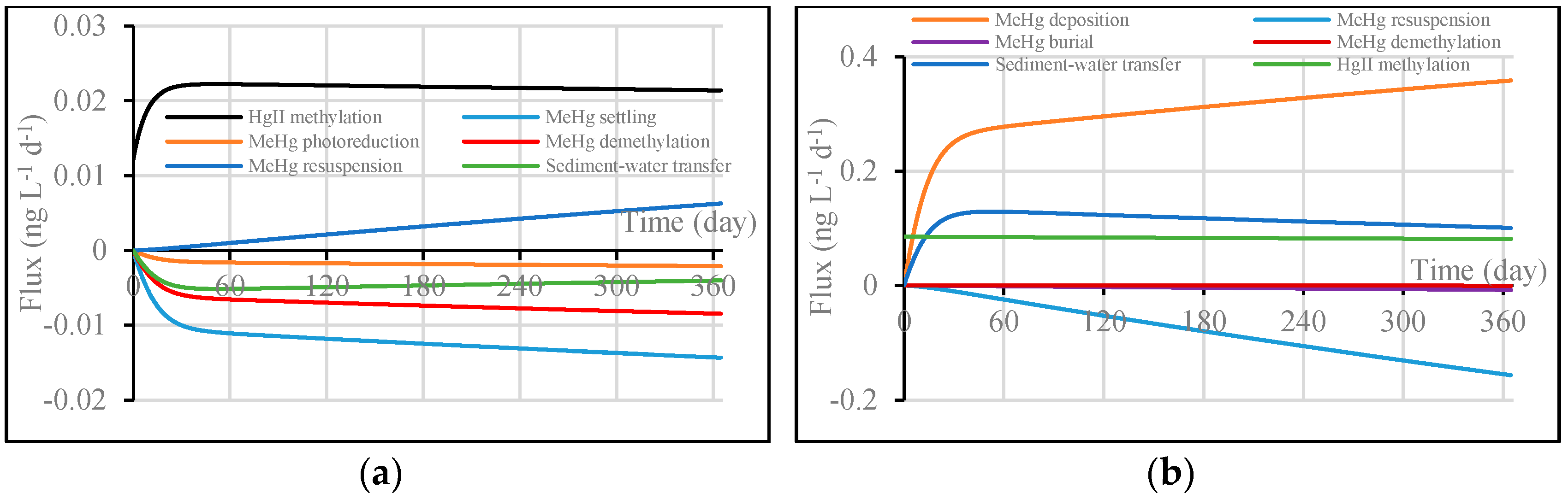
Figure 5a,b show the comparison of W2 and WASP computed concentrations of MeHg in the water column and sediment layer. Figure 6a,b show W2 computed MeHg internal flux by each process. MeHg main source was from the methylation of HgII in the water column. Settling and resuspension were not the dominant processes affect the fate of MeHg in the water column. In the sediment layer, main sources of MeHg come from MeHg deposition from water column and HgII methylation. It is important to understand the sources of MeHg in order to control the production of MeHg in the water column and sediment layer and reduce the environmental risk.
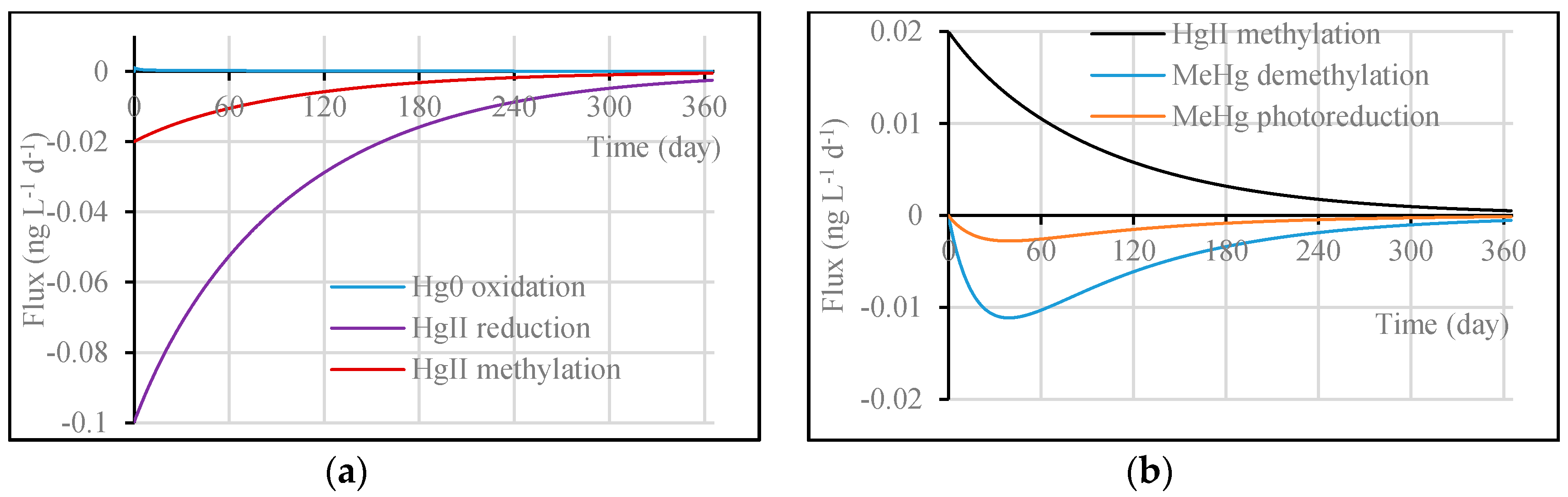
To investigate individual Hg transformations, solid sorption, settling, resuspension, and sediment-water transfer processes were turned off. Figure 7a,b show dissolved concentrations of HgII and MeHg in the water column. Figure 8a,b show Hg transformation fluxes respectively. W2 predicted concentrations of HgII and MeHg are consistent with WASP model results. Dissolved HgII was lost by its reduction and methylation in the water column. In the meantime, MeHg was gained and reached the peak around 50 days, then decreased by its demethylation and photoreduction. The above case studies indicate that the algorithms and formulations were correctly implemented in the enhanced W2 model.
3.2. Application and Evaluation of the Enhanced W2 Model
3.2.1. Study Area
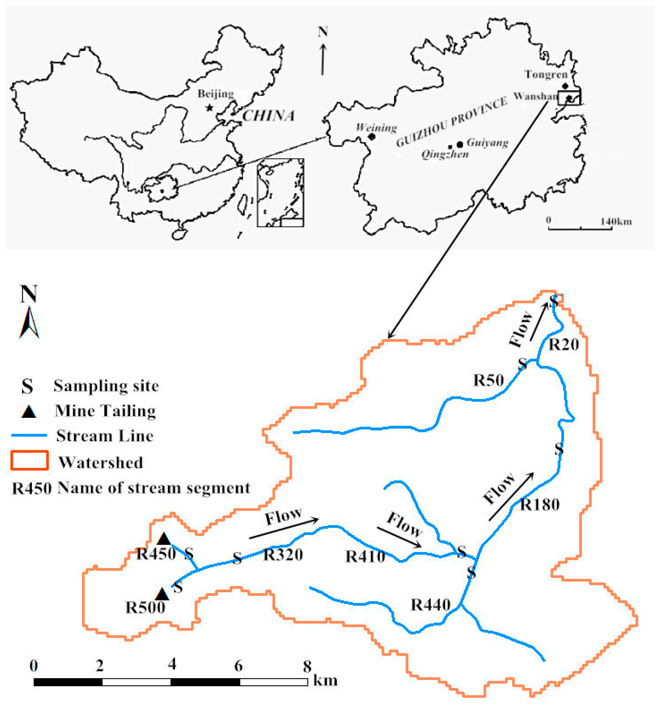
The Xiaxi River is located in Wanshan County, Guizhou Province, China. This river has been influenced by the world-famous Wanshan Hg mining, which is one of the thirteen large and super large-scale Hg mines located within the Guizhou Province, China. Figure 9 shows the extent of the Xiaxi River, and its location in Guizhou Province. The Hg tailings are distributed throughout the headwater reaches of the Xiaxi River. Due to the high geochemical background of Hg in this area and high Hg emissions from coal combustion using Hg enriched coals as well as from mining activities, Hg contamination in this area has become a concern [43,44,45,46].
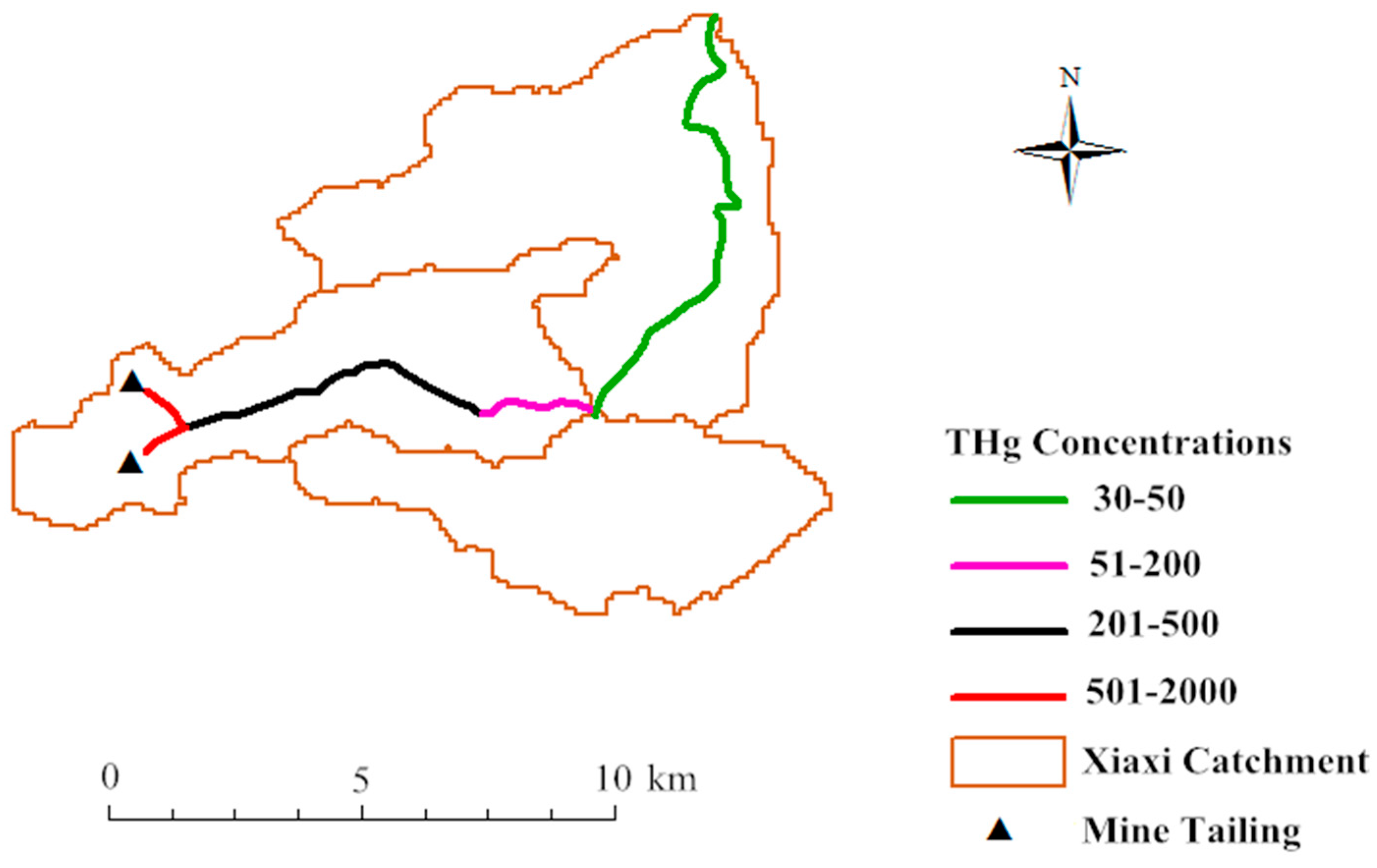
Water samples were respectively collected at the eight sampling sites in the watercourse (Figure 9) during moderate and high flow periods in 2007 and 2008 [47,48]. Concentrations of THg, dissolved mercury (DHg), MeHg and total suspended solids (TSS) were measured in the laboratory for all collected samples. The collection, storage, and preservation techniques of samples complied with the USEPA Method 1631. Figure 10 shows the distribution of 2008’s observed THg concentrations in the watercourse of the Xiaxi River system. The THg concentrations were much higher along the Xiaxi River and then decreased rapidly downstream from the source. Based on observed data collected in 2007 and 2008, the THg concentrations ranged in the surface water from 4.5 to 2100 ng·L−1 [47,49]. The THg concentrations in the benthic sediments ranged from 1.1 to 360 mg·kg−1 [49].
3.2.2. Model Development and Calibration
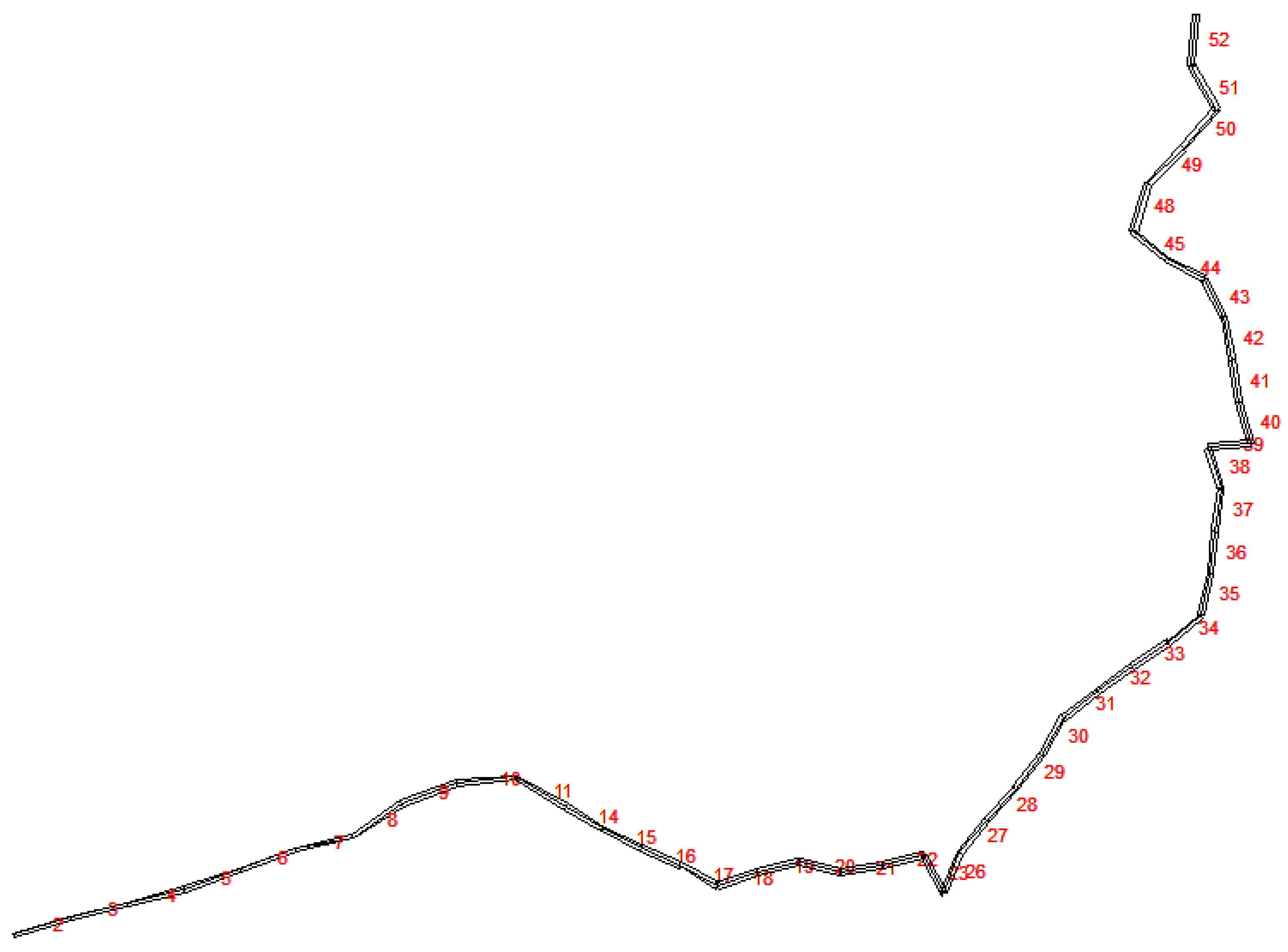
The W2 model was applied to the mainstem Xiaxi River from the headwater until the outlet of the watershed (Figure 9). The mainstem river is about 17 km long. The Xiaxi River is across the whole watershed and has been the main concern of Hg contamination. Table 4 listed the geometry of the Xiaxi River reaches and major tributaries. The Xiaxi River W2 model mainly consists of reaches R320, R410, R180 and R20 (Figure 9). River reaches R450 and R500 were treated as Hg contaminated sources, and R50 and R440 were treated as uncontaminated sources. The plan view of the Xiaxi River W2 model grid is shown in Figure 11. The Xiaxi River was discretized with fifty-three horizontal segments with Δx ranging from 338.8 to 468.7 m. The averaged water depth was 0.5 m. The vertical layer thickness was set up with 0.25 m.
The inputs used for the Xiaxi River W2 model include external loads, initial and boundary conditions, and water quality parameters. The input data were assembled based on field data collected during the project period (2007–2008), outputs generated from other models, and literatures. Because Xiaxi River lacks routine hydrological monitoring, the HEC-HMS model was used to compute the stream flow [18] and fed into the W2 model. Xiaxi River inflow discharges for reaches R450, R500, R50 and R440 are shown in Figure 12a,b.
Two suspended solids (fine and coarse solids) were simulated to characterize the partitioning and distribution of HgII and MeHg along the river. The fine solids represent particles with corresponding particle diameter of 0.01 mm, and the coarse solids represent particles with corresponding particle diameter of 0.1 mm. Figure 13 shows the solids grading curves of four sampling sites in the river. Fine solids account for 88.5% of the TSS. The boundary conditions of TSS and THg were calculated based on the following linear regression relationships developed by Lin et al. [18].
where Q is the stream flow (m3·s−1), TSS is total suspended solids (mg·L−1), THg is the total concentration (ng·L−1).
Based on available observed data, the Xiaxi River W2 model was calibrated in several steps. First, the manning’s roughness coefficient ‘n’ was calibrated so that simulated discharge approximated observed flow discharge [18]. The final manning’s roughness coefficient ‘n’ was set as 0.035. Next, the settling velocities of fine and coarse particles were calibrated, and simulated TSS approximated observed TSS concentrations along the river. In the Hg simulation module, the partitioning coefficients and transformation rates for HgII and MeHg were calibrated through a sensitivity analysis. Finally, the W2 model performance was evaluated by root mean square error (RMSE) and relative error (RE).
where CM is the modeled concentration (ng·L−1 for Hg and mg·L−1 for TSS), CO is the observed concentration (ng·L−1 for Hg and mg·L−1 for TSS).
3.2.3. Results and Discussion
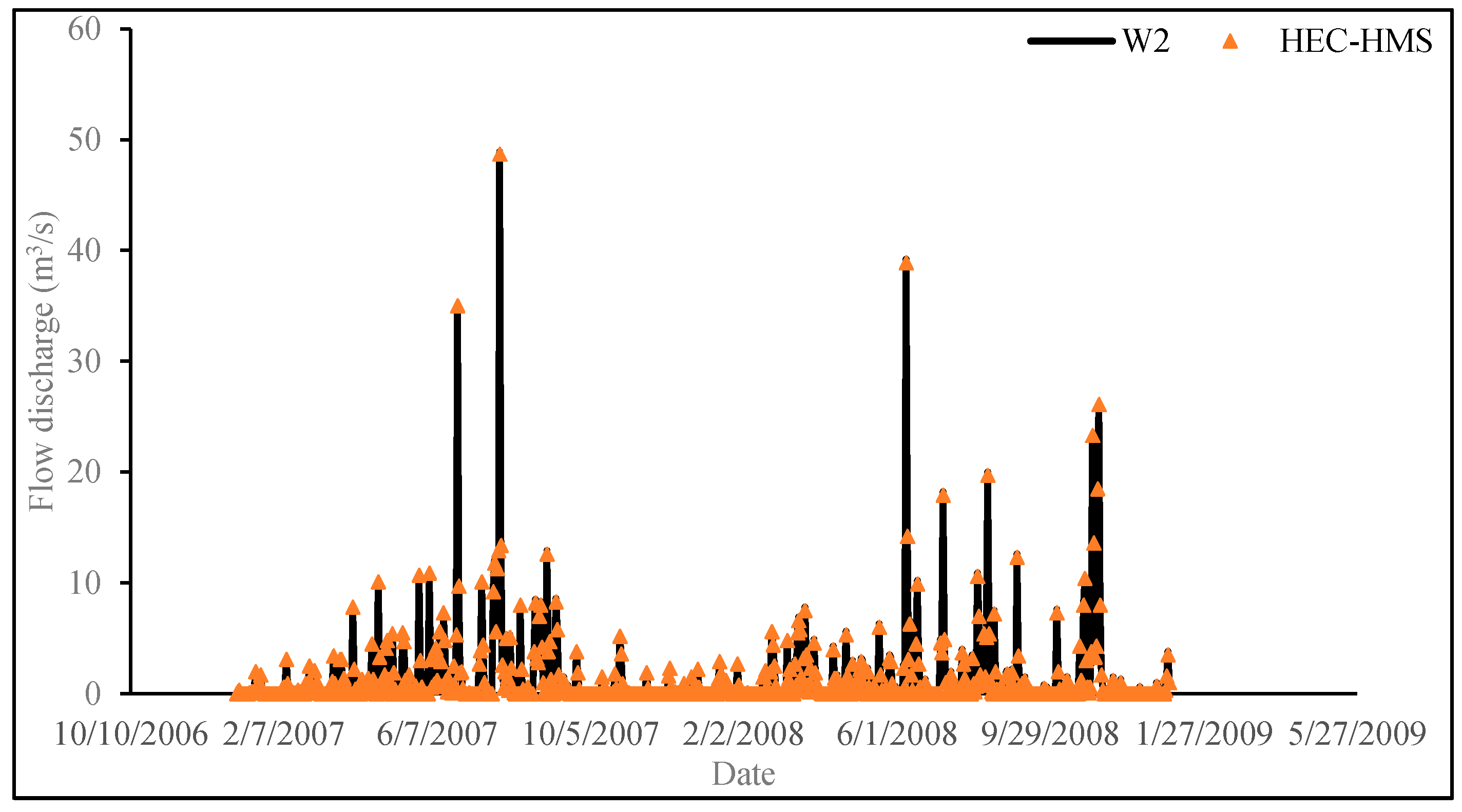
Figure 14 presents the comparison of W2 simulated flow discharge and simulated data [18] at the mouth of the Xiaxi River. The average error is 0.12 m3/s. High flood events mainly took place during the summer time (June to August), which were consistent with observed rainfall events. The W2 model was able to reproduce observed hydrodynamic results in the river.
After the hydrodynamics was calibrated, the W2 model was further calibrated for suspended solids. The modeled TSS concentrations were compared with observed data in Table 5. The results show that the RMSE for TSS is 0.10 mg·L−1 in 4 September 2007, and the relative error is 10%. For the TSS in 8 August 2008, the RMSE is 0.081 mg L−1, and the relative error is 2.62%. The RMSE and RE values in high flow period are much lower than that in moderate flow period. The RE value increased when TSS concentration decreased, especially when TSS concentration is lower than 1.0 mg·L−1. The settling velocities of fine and coarse particles with 5 m·d−1 and 25 m d−1 were used in the model.
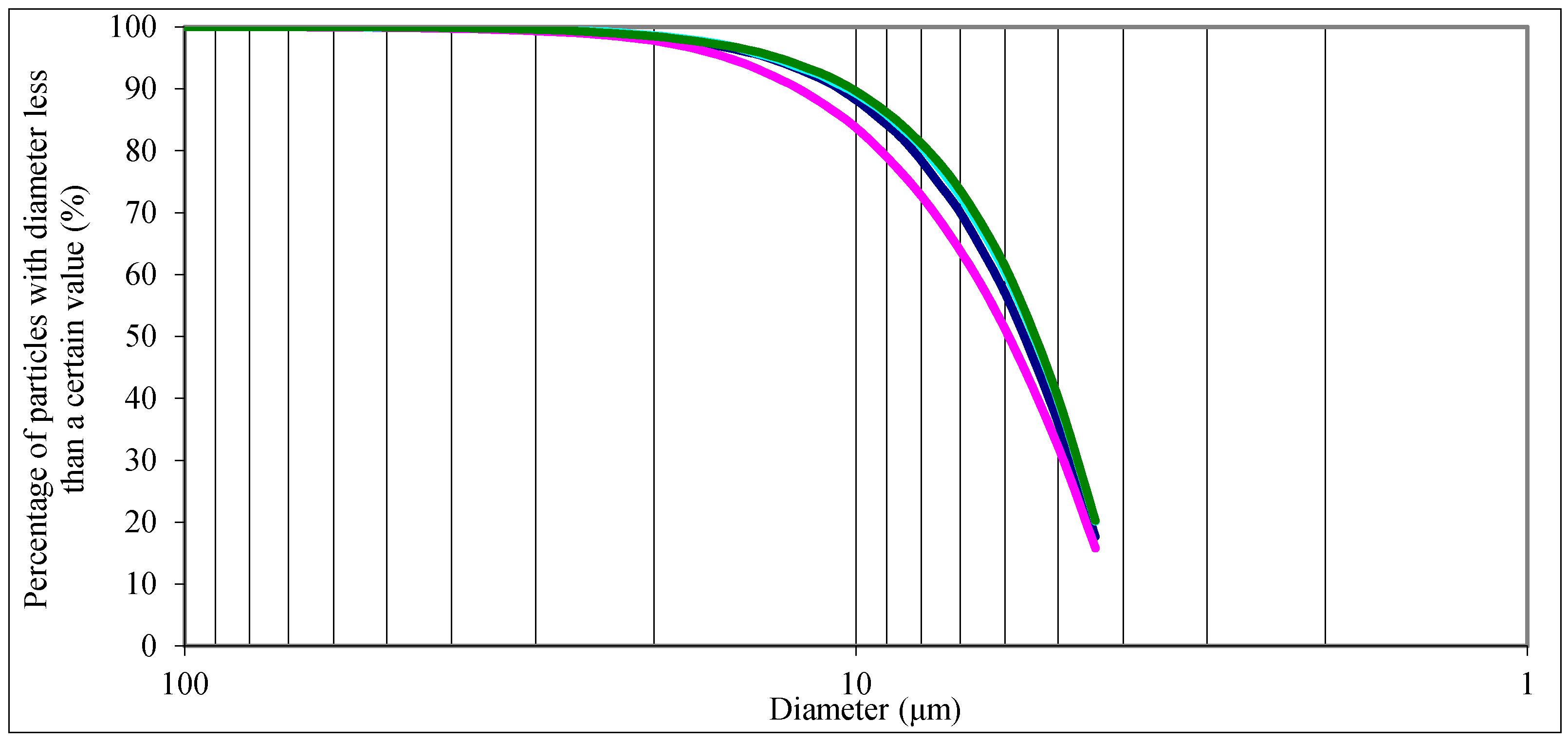
The partitioning coefficient of Hg on inorganic solids has a wide range in literatures. Allison and Allison [41] provided a range of 102–106 L·kg−1. From a study of several Wisconsin lakes conducted by Rice et al. [50], the partitioning coefficient of Hg ranged from 8 × 10⁴ to 3.4 × 10⁵. Suggested values for both methylation and demethylation rates are 10−5–10−2 d−1 [41]. Methylation rate ranged between 0.01 to 0.09 d−1 in a clear lake in Wisconsin [51]. Studies by Carroll et al. [52] and Oremland et al. [53] indicated that methylation rates in Carson River ranged between 0.0025 and 0.011 d−1 and demethylation rates ranged between 0.12 and 0.55 d−1. A sensitivity analysis was performed using a range of partitioning coefficient (Kd) and methylation/demethylation rate (M/D). W2 modeled DHg and MeHg concentrations with a range of values of Kd and M/D are presented in Table 6 and Table 7. Based on the sensitivity analysis, the partitioning coefficients of Hg on fine and coarse solids were set to 106 and 104 L·kg−1. The methylation and demethylation rates were set to 0.01 and 0.1 d−1 in this study.
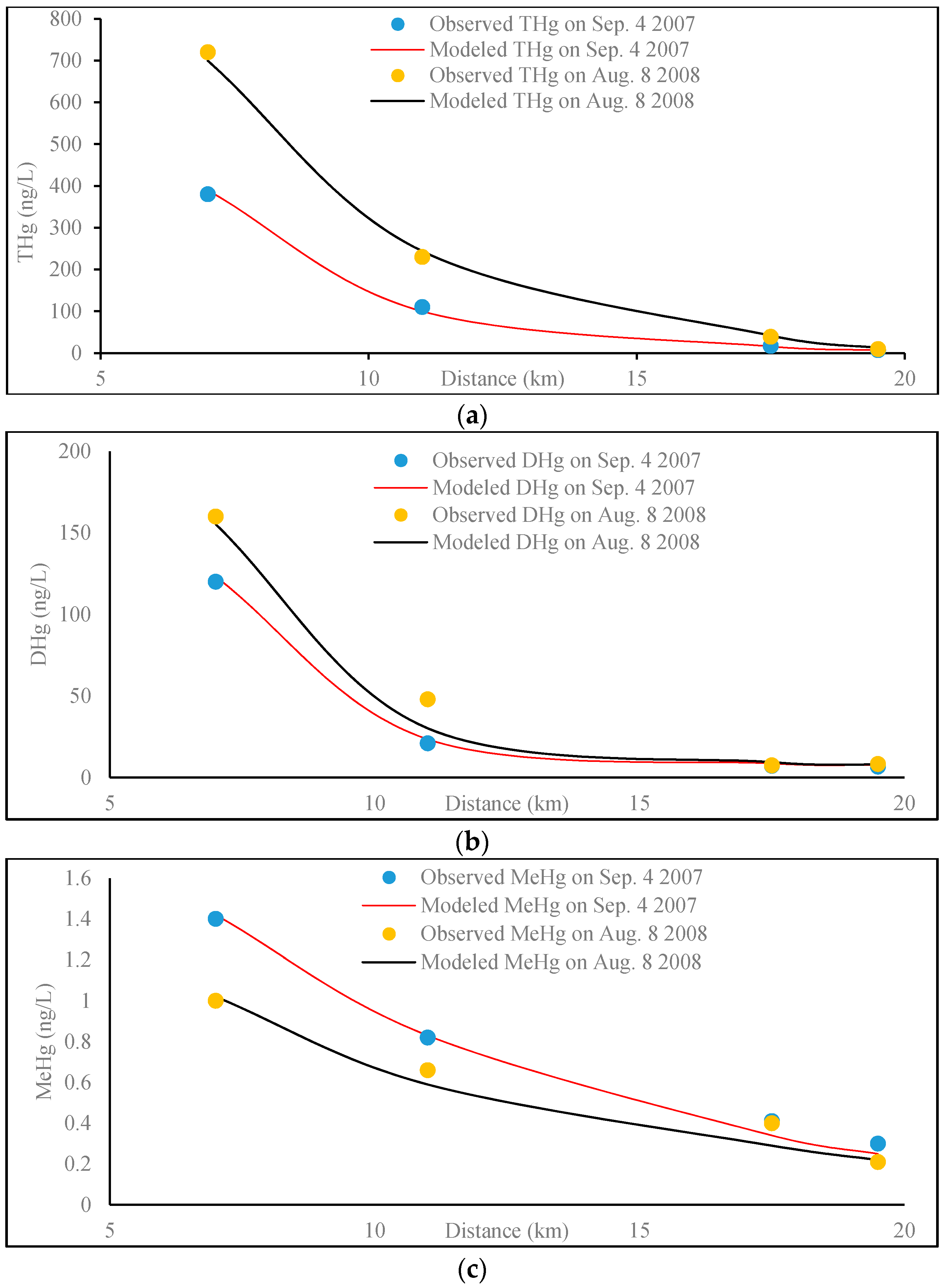
Figure 15 presents the comparisons of W2 computed Hg concentrations (THg, DHg and MeHg) and observed data along the mainstem Xiaxi River from tailings during September 2007 and August 2008. The concentrations of THg, DHg and MeHg decreased rapidly along the river. The model predicted concentrations of Hg species were reasonable well when compared with observed data. The RMSE and RE values of modeled THg were 13.0 ng·L−1 and 7.7% in September 2007, and 19.0 ng·L−1 and 7.2% in August 2008. The RMSE and RE values of modeled DHg were 3.8 ng·L−1 and 9.0% in September 2007, and 10.0 ng·L−1 and 13% in August 2008. The RMSE and RE values of modeled MeHg were 0.07 ng·L−1 and 7.4% in September 2007, and 0.09 ng·L−1 and 11% in August 2008. The particulate fractions took account of more than 75% of THg concentrations for all sampling sites, and the MeHg concentration dissolved in water was much lower than THg.
4. Summary and Conclusions
The Hg simulation module has been developed and incorporated into the 2D hydrodynamic and water quality model CE-QUAL-W2. The enhanced W2 model was tested and validated against WASP mercury model. The model results indicated that the enhanced W2 model was well designed, and the algorithms and formulations were correctly implemented. Application of the enhanced W2 model to the Xiaxi River, a river course in Wanshan Hg mining area of Guizhou Province, China, further evaluated the capability of the enhanced W2 model to simulate the transport and cycling of Hg in water bodies. The enhanced W2 model was able to reproduce observed TSS, THg, DHg and MeHg. THg, DHg and MeHg concentrations decreased rapidly downstream from the source and stabilized at lower levels, which is likely due to high association of Hg to solids and the rapid settlement of these solids. The source control of Hg discharge is the key to reduce the Hg contamination along the Xiaxi River. This application demonstrated the W2 model capability in predicting complex transport and cycling of Hg species in water bodies. When more observed data become available, the robustness of the Xiaxi River W2 model will be further calibrated and validated. The current model can also be used to perform scenarios analysis and quantify the best management practice for the XiaXi River.
Acknowledgments
This study was supported by NSFC (51479219) and Program for Innovative Research Team of IWHR. The authors thank Yan Lin in Norwegian Institute for Water Research for providing Xiaxi River flow and mercury dataset. The pertinent comments by the two reviewers were fully acknowledged here.
Author Contributions
Senlin Zhu performed the model programming, data analysis and calculation; Zhonglong Zhang and Xiaobao Liu lead the model development and supervised the study.
Conflicts of Interest
The authors declare no conflict of interest.
References
- Martin, J.L. Application of two-dimensional water quality model. J. Environ. Eng. 1988, 114, 317–336. [Google Scholar] [CrossRef]
- Cole, T.M.; Wells, S.A. CE-QUAL-W2: A Two-Dimensional, Laterally Averaged, Hydrodynamic and Water Quality Model, Version 3.71; Portland State University: Portland, OR, USA, 2011. [Google Scholar]
- Kim, Y.; Kim, B. Application of a 2-dimensional water quality model (CE-QUAL-W2) to the turbidity interflow in a deep reservoir (Lake Soyang, Korea). Lake Reserv. Manag. 2006, 22, 213–222. [Google Scholar] [CrossRef]
- Debele, B.; Srinivasan, R.; Parlange, J.Y. Coupling upland watershed and downstream waterbody hydrodynamic and water quality models (SWAT and CE-QUAL-W2) for better water resources management in complex river basins. Environ. Model. Assess. 2008, 13, 135–153. [Google Scholar] [CrossRef]
- Afshar, A.; Kazemi, H.; Saadatpour, M. Particle swarm optimization for automatic calibration of large scale water quality model (CE-QUAL-W2): Application to Karkheh reservoir, Iran. Water Resour. Manag. 2011, 25, 2613–2632. [Google Scholar] [CrossRef]
- Ma, J.; Liu, D.; Wells, S.A.; Tang, H.; Ji, D.; Yang, Z. Modeling density currents in a typical tributary of the Three Gorges Reservoir, China. Ecol. Model. 2015, 296, 113–125. [Google Scholar] [CrossRef]
- Noori, R.; Yeh, H.-D.; Ashrafi, K.; Rezazadeh, N.; Bateni, S.M.; Karbassi, A.; Kachoosangi, F.T.; Moazami, S. A reduced-order based CE-QUAL-W2 model for simulation of nitrate concentration in dam reservoirs. J. Hydrol. 2015, 530, 645–656. [Google Scholar] [CrossRef]
- Brown, C.A.; Sharp, D.; Collura, T.C. Effect of climate change on water temperature and attainment of water temperature criteria in the Yaquina Estuary, Oregon (USA). Estuar. Coast. Shelf Sci. 2016, 169, 136–146. [Google Scholar] [CrossRef]
- Zhang, Z.; Sun, B.; Johnson, B.E. Integration of a benthic sediment diagenesis module into the two dimensional hydrodynamic and water quality model—CE-QUAL-W2. Ecol. Model. 2015, 297, 213–231. [Google Scholar] [CrossRef]
- Keating, M.H.; Mahaffey, K.R.; Schoeny, R.; Rice, G.E.; Bullock, O.R. Mercury Study Report to Congress; Volume I. Executive Summary. 1997. Available online: https://www3.epa.gov/airtoxics/112nmerc/volume1.pdf (accessed on 1 July 2017).
- US EPA (U.S. Environmental Protection Agency). Guidance for Assessing Chemical Contaminant Data for Use in Fish Advisories Volume 2 Risk Assessment and Fish Consumption Limits. 2000. Available online: https://www.epa.gov/sites/production/files/2015-06/documents/volume2.pdf (accessed on 1 July 2017).
- EFSA (European Food Safety Authority). EFSA Provides Risk Assessment on Mercury in Fish: Precautionary Advice Given to Vulnerable Groups, Press Release. 18 March 2004. Available online: https://www.efsa.europa.eu/fr/press/news/contam040318 (accessed on 1 July 2017).
- Hudson, R.J.M.; Gherini, S.A.; Watras, C.J.; Porcella, D.S. Modeling the biogeochemical cycle of mercury in lakes: The mercury cycling model (MCM) and its application to the MTL study lakes. In Mercury Pollution—Integration and Synthesis; Lewis Publishers: Ann Arbor, MI, USA, 1994; pp. 473–523. [Google Scholar]
- Martin, J.L. MERC4: A Mercury Transport and Kinetics Model (beta 1.0); U.S. Environmental Protection Agency, Center for Exposure Assessment Modeling: Athens, GA, USA, 1992.
- Knightes, C.D. Development and test application of a screening-level mercury fate model and tool for evaluating wildlife exposure risk for surface waters with mercury-contaminated sediments (SERAFM). Environ. Model. Softw. 2008, 23, 495–510. [Google Scholar] [CrossRef]
- Wool, T.A.; Ambrose, R.B.; Martin, J.L.; Comer, E.A. Water Quality Analysis Simulation Program (WASP), Version 6, User’s Manual; U.S. Environmental Protection Agency: Athens, GA, USA, 2006.
- Knightes, C.D.; Sunderland, E.M.; Barber, M.C.; Johnston, J.M.; Ambrose, R.B. Application of ecosystem-scale fate and bioaccumulation models to predict fish mercury response times to changes in atmospheric deposition. Environ. Toxicol. Chem. 2009, 28, 881–893. [Google Scholar] [CrossRef] [PubMed]
- Lin, Y.; Larssen, T.; Vogt, R.D.; Feng, X.B.; Zhang, H. Modelling transport and transformation of mercury fractions in heavily contaminated mountain streams by coupling a GIS-based hydrological model with a mercury chemistry model. Sci. Total Environ. 2011, 409, 4596–4605. [Google Scholar] [CrossRef] [PubMed]
- Turner, D.R. Speciation cycling of arsenic, cadmium, lead and mercury in natural waters. In Lead, Mercury, Cadmium and Arsenic in the Environment; John Wiley & Sons Ltd.: Hoboken, NJ, USA, 1987; pp. 175–186. [Google Scholar]
- Stein, E.D.; Cohen, Y.; Winer, A.M. Environmental distribution and transformation of mercury compounds. Crit. Rev. Environ. Sci. Technol. 1996, 26, 1–43. [Google Scholar] [CrossRef]
- Jackson, T.A. Long-range atmospheric transport of mercury to ecosystems, and the importance of anthropogenic emissions: A critical review and evaluation of the published evidence. Environ. Rev. 1997, 5, 99–120. [Google Scholar] [CrossRef]
- Morel, F.M.M.; Kraepiel, A.M.L.; Amyot, M. The chemical cycle and bioaccumulation of mercury. Annu. Rev. Ecol. Syst. 1998, 29, 543–566. [Google Scholar] [CrossRef]
- Zhang, Z.; Johnson, B.E. Aquatic Contaminant and Mercury Simulation Modules Developed for Hydrological and Hydraulic Models; ERDC/EL TR-16-8; US Army Engineer Research and Development Center: Vicksburg, MS, USA, 2016.
- Schroeder, W.H.; Munthe, J. Atmospheric mercury—An overview. Atmos. Environ. 1998, 32, 809–822. [Google Scholar] [CrossRef]
- Thibodeaux, L.J.; Valsaraj, K.T.; Reible, D.D. Bioturbation-driven transport of hydrophobic organic contaminants from bed sediment. Environ. Eng. Sci. 2001, 18, 215–223. [Google Scholar] [CrossRef]
- Ditoro, D.M. Sediment Flux Modeling; Wiley-Interscience: New York, NY, USA, 2001. [Google Scholar]
- Boyer, J.M.; Chapra, S.C.; Ruiz, C.E.; Dortch, M.S. RECOVERY: A Mathematical Model to Predict the Temporal Response of Surface Water to Contaminated Sediments; U.S. Army Corps of Engineers Waterways Experiment Station: Vicksburg, MS, USA, 1994.
- Schink, D.R.; Guinasso, N.L. Modelling the influence of bioturbation and other processes on calcium carbonate dissolution at the sea floor. In The Fate of Fossil Fuel CO2 in the Oceans; Plenum Press: New York, NY, USA, 1977; pp. 375–399. [Google Scholar]
- Feng, X.; Qiu, G. Mercury pollution in Guizhou, Southwestern China—An overview. Sci. Total Environ. 2008, 400, 227–237. [Google Scholar] [CrossRef] [PubMed]
- Qiu, G.L.; Feng, X.B.; Wang, S.F.; Shang, L.H. Mercury and methylmercury in riparian soil, sediments, mine-waste calcines, and moss from abandoned Hg mines in east Guizhou province, southwestern China. Appl. Geochem. 2005, 20, 627–638. [Google Scholar] [CrossRef]
- King, J.K.; Michael, S.F.; Lee, R.F.; Jahnke, R.A. Coupling mercury methylation rates to sulfate reduction rates in marine sediments. Environ. Toxicol. Chem. 1999, 18, 1362–1369. [Google Scholar] [CrossRef]
- Gilmour, C.C.; Elias, D.A.; Kucken, A.M.; Brown, S.D.; Palumbo, A.V.; Wall, J.D. Sulfate-reducing bacterium Desulfovibrio desulfuricans ND132 as a model for understanding bacterial mercury methylation. Appl. Environ. Microbiol. 2011, 77, 3938–3951. [Google Scholar] [CrossRef] [PubMed]
- Achá, D.; Hintelmann, J.; Yee, J. Importance of sulfate reducing bacteria in mercury methylation and demethylation in periphyton from Bolivian Amazon region. Chemosphere 2011, 82, 911–916. [Google Scholar] [CrossRef]
- Shao, D.; Kang, Y.; Wu, S.; Wong, M.H. Effects of sulfate reducing bacteria and sulfate concentrations on mercury methylation in freshwater sediments. Sci. Total Environ. 2012, 424, 331–336. [Google Scholar] [CrossRef] [PubMed]
- Zhang, T.; Hsukim, H. Photolytic degradation of methylmercury enhanced by binding to natural organic ligands. Nat. Geosci. 2010, 3, 473–476. [Google Scholar] [CrossRef] [PubMed]
- He, F.; Zheng, W.; Liang, L.; Gu, B. Mercury photolytic transformation affected by low-molecular-weight natural organics in water. Sci. Total Environ. 2012, 416, 429–435. [Google Scholar] [CrossRef] [PubMed]
- Fleck, J.A.; Gill, G.; Bergamaschi, B.A.; Kraus, T.E.; Downing, B.D.; Alpers, C.N. Concurrent photolytic degradation of aqueous methylmercury and dissolved organic matter. Sci. Total Environ. 2014, 484, 263–275. [Google Scholar] [CrossRef] [PubMed]
- Seo, D.; Kim, M.; Ahn, J.H. Prediction of Chlorophyll-a Changes due to Weir Constructions in the Nakdong River Using EFDC-WASP Modelling. Environ. Eng. Res. 2012, 17, 95–102. [Google Scholar] [CrossRef]
- Xiao, D.; Jia, H.; Wang, Z. Modeling Megacity Drinking Water Security under a DSS Framework in a Tidal River at the North Pearl River Delta, China. J. Am. Water Resour. Assoc. 2015, 51, 637–654. [Google Scholar] [CrossRef]
- Chen, C.X.; Zheng, B.H.; Jiang, X.; Zhao, Z.; Zhan, Y.Z.; Yi, F.J.; Ren, J.Y. Spatial distribution and pollution assessment of mercury in sediments of Lake Taihu, China. J. Environ. Sci. 2013, 25, 316–325. [Google Scholar] [CrossRef]
- Allison, J.D.; Allison, T.L. Partition Coefficients for Metals in Surface Water, Soil, and Waste; EPA-600/R-05/074; Rep. U.S. Environmental Protection Agency, Office of Research and Development: Washington DC, USA, 2005.
- Muresan, B.; Cossa, D.; Richard, S.; Burban, B. Mercury speciation and exchanges at the air-water interface of a tropical artificial reservoir, French Guiana. Sci. Total Environ. 2007, 385, 132–145. [Google Scholar] [CrossRef] [PubMed]
- Pacyna, E.G.; Pacyna, J.M. Global emission of mercury from anthropogenic sources in 1995. Water Air Soil Pollut. 2002, 137, 149–165. [Google Scholar] [CrossRef]
- Pacyna, J.M.; Breivik, K.; Münch, J.; Fudala, J. European atmospheric emissions of selected persistent organic pollutants, 1970–1995. Atmos. Environ. 2003, 37, 119–131. [Google Scholar] [CrossRef]
- Dastoor, A.P.; Larocque, Y. Global circulation of atmospheric mercury: A modelling study. Atmos. Environ. 2004, 38, 147–161. [Google Scholar] [CrossRef]
- Feng, X. Mercury pollution in China—An Overview. In Dynamics of Mercury Pollution on Regional and Global Scales; Springer: New York, NY, USA, 2005; pp. 657–678. [Google Scholar]
- Zhang, H.; Feng, X.; Larssen, T.; Shang, L.; Vogt, R.D.; Rothenberg, S.E.; Li, P.; Zhang, H.; Lin, Y. Fractionation, distribution and transport of mercury in rivers and tributaries around Wanshan Hg mining district, Guizhou province, southwestern China: Part 1—Total mercury. Appl. Geochem. 2010, 25, 633–641. [Google Scholar] [CrossRef]
- Zhang, H.; Feng, X.; Larssen, T.; Shang, L.; Vogt, R.D.; Lin, Y.; Li, P.; Zhang, H. Fractionation, distribution and transport of mercury in rivers and tributaries around Wanshan Hg mining district, Guizhou province, southwestern China: Part 2—Methyl mercury. Appl. Geochem. 2010, 25, 642–649. [Google Scholar] [CrossRef]
- Lin, Y.; Larssen, T.; Vogt, R.D.; Feng, X.B. Identification of fractions of mercury in water, soil and sediment from a typical Hg mining area in Wanshan, Guizhou province, China. Appl. Geochem. 2010, 25, 60–68. [Google Scholar] [CrossRef]
- Rice, G.E.; Ambrose, R.B.; Bullock, O.R.; Swartout, J. Mercury Study Report to Congress. Volume 3. Fate and Transport of Mercury in the Environment. 1997. Available online: https://www3.epa.gov/airtoxics/112nmerc/volume3.pdf (accessed on 1 July 2017).
- Eckley, C.S.; Watras, C.J.; Hintelmann, H.; Morrison, K.; Kent, A.D.; Regnell, O. Mercury methylation in the hypolimnetic waters of lakes with and without connection to wetlands in northern Wisconsin. Can. J. Fish. Aquat. Sci. 2005, 62, 400–411. [Google Scholar] [CrossRef]
- Carroll, R.W.H.; Warwick, J.J.; Heim, K.J.; Bonzongo, J.C.; Miller, J.R.; Lyons, W.B. Simulation of mercury transport and fate in the Carson River, Nevada. Ecol. Model. 2000, 125, 255–278. [Google Scholar] [CrossRef]
- Oremland, R.S.; Miller, L.G.; Dowdle, P.; Connell, T.; Barkay, T. Methyl-mercury oxidative degradation potentials in contaminated and pristine sediments of the Carson River, Nevada. Appl. Environ. Microbiol. 1995, 61, 2745–2753. [Google Scholar] [PubMed]
Figure 1.
Conceptual representation of Hg speciation and processes modeled in the W2 model.

Figure 2.
Flow chart of the W2 model solving the transport and mass balance of three Hg species.
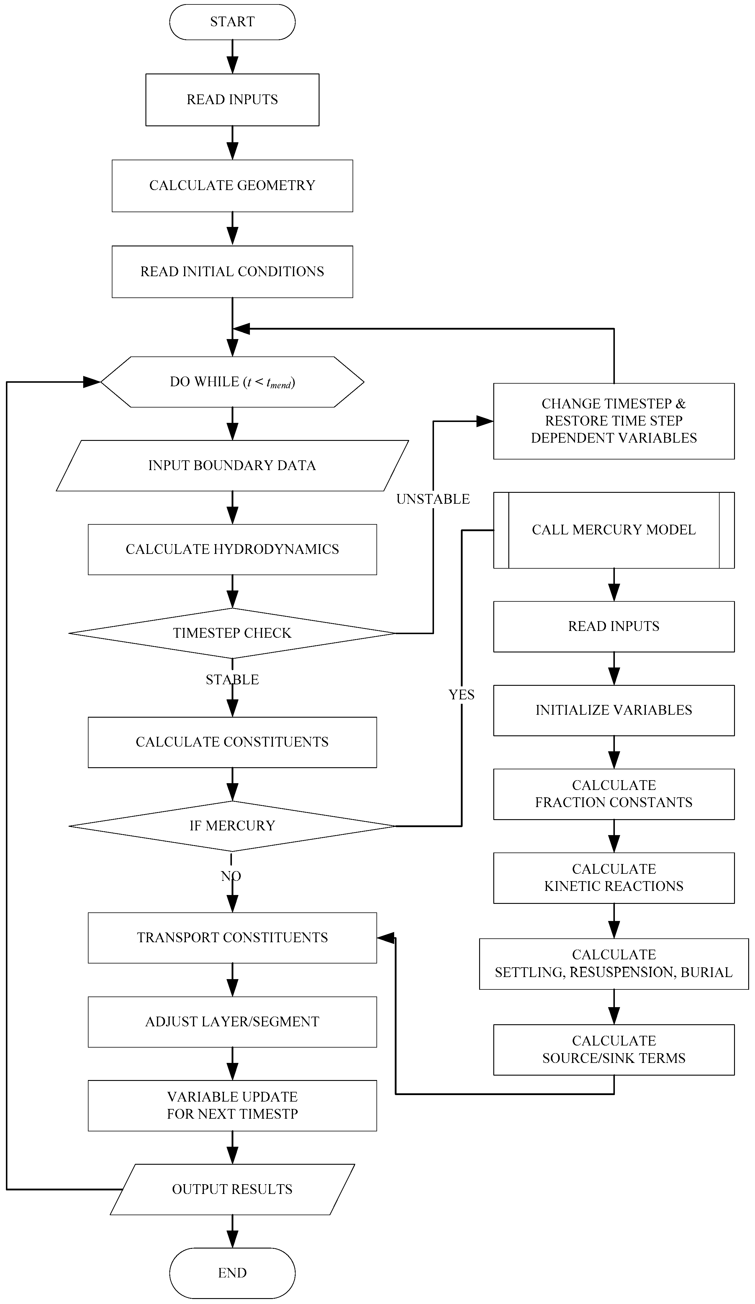
Figure 3.
W2 and WASP computed HgII distributed concentrations in the water column (a) and the sediment layer (b): HgII (concentration of total HgII in water); HgIId (concentration of dissolved HgII in water); HgIIpts (total concentration of solids adsorbed HgII in water); HgII2 (concentration of total HgII in sediment); HgIId2 (concentration of dissolved HgII in sediment).
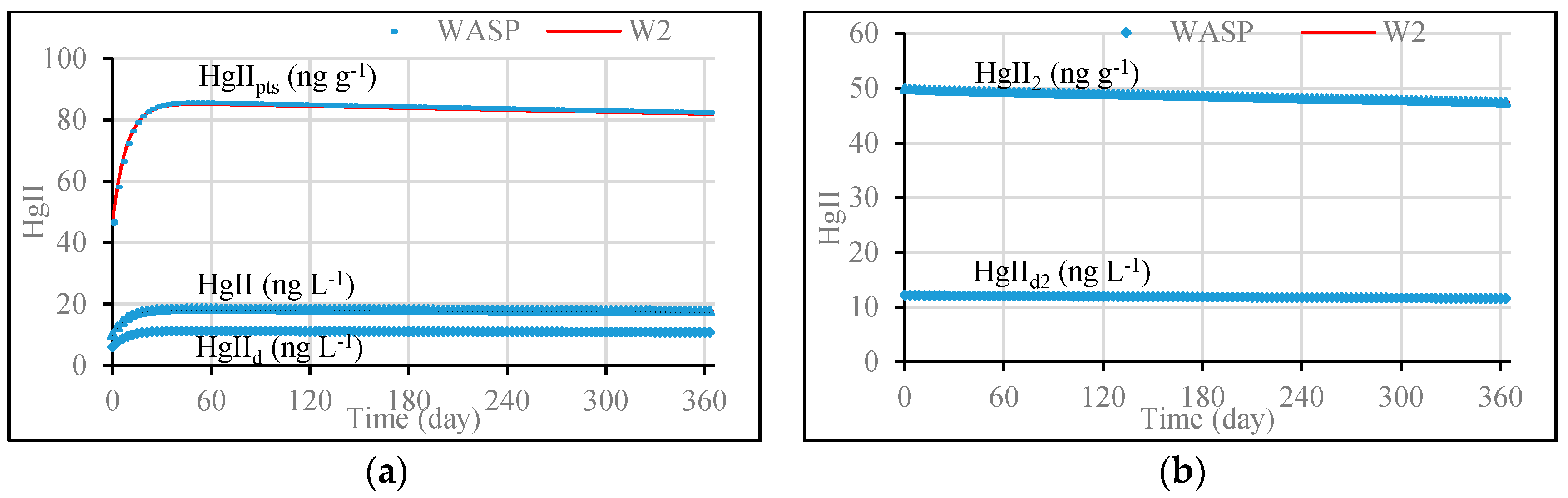
Figure 4.
W2 computed HgII internal fluxes in the water column (a) and the sediment layer (b).
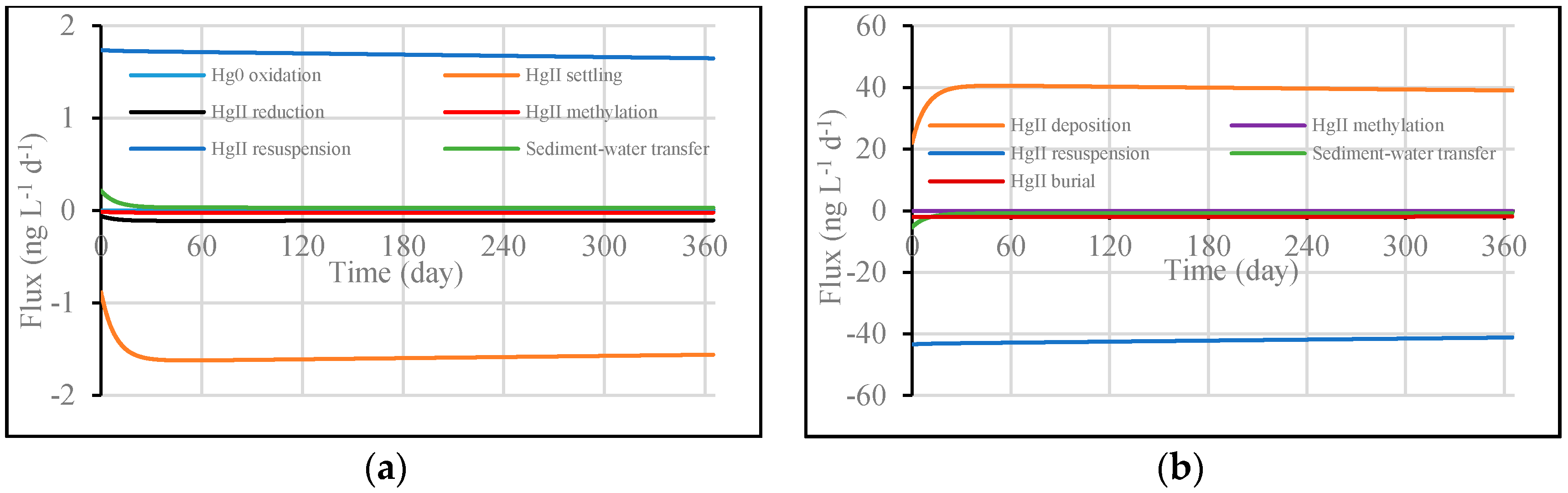
Figure 5.
W2 and WASP computed MeHg distributed concentrations in the water column (a) and the sediment layer (b): MeHg (concentration of total MeHg in water); MeHgd (concentration of dissolved MeHg in water); MeHgpts (total concentration of solids adsorbed MeHg in water); MeHg2 (concentration of total MeHg in sediment); MeHgd2 (concentration of dissolved MeHg in sediment).
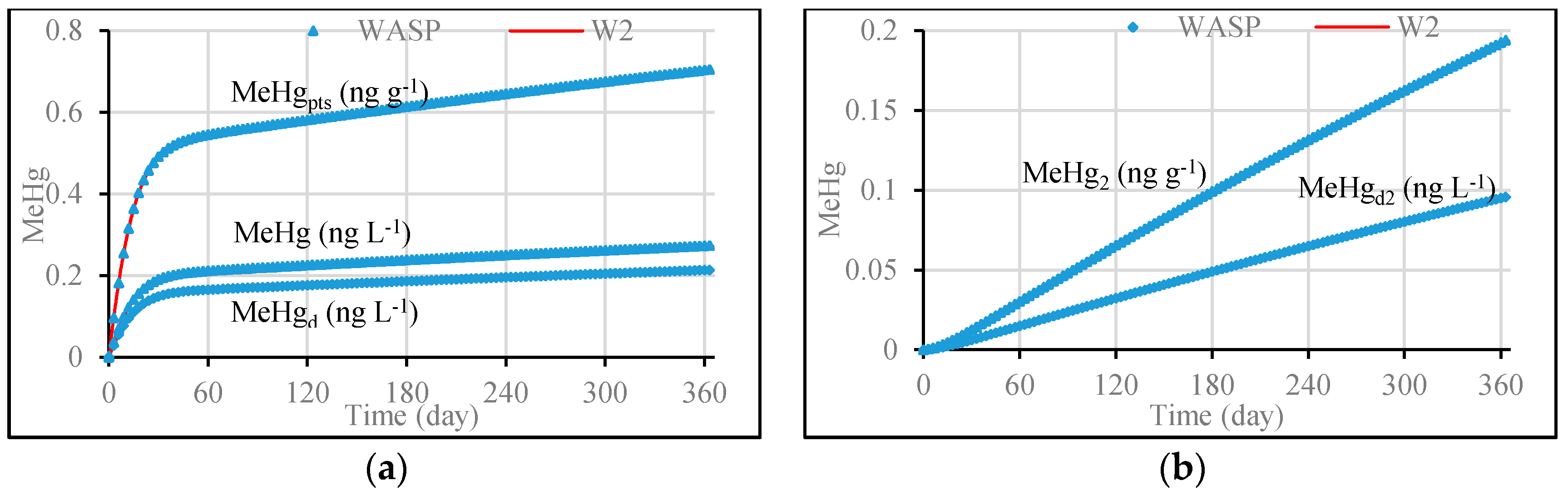
Figure 6.
W2 computed MeHg internal fluxes in the water column (a) and the sediment layer (b).

Figure 7.
W2 and WASP computed (a) HgII and (b) MeHg concentrations in the water column.
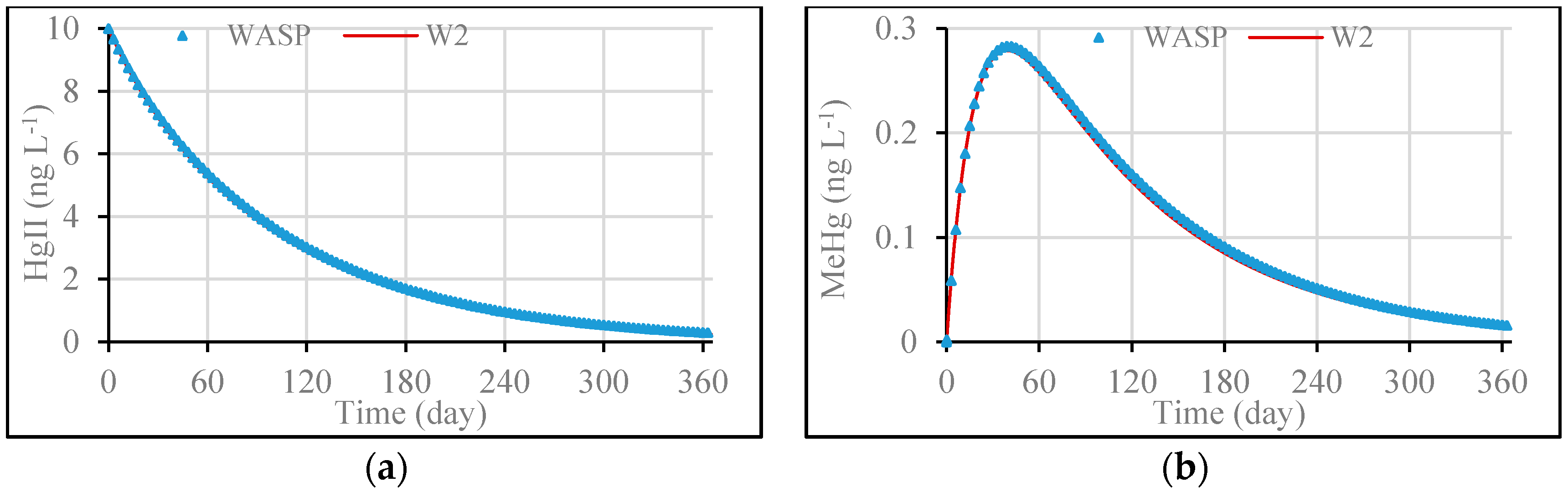
Figure 8.
W2 computed (a) HgII and (b) MeHg concentrations and internal fluxes in the water column.

Figure 9.
Map of the Xiaxi River watershed and sampling sites.

Figure 10.
Spatial distribution of THg concentrations along the watercourse of Xiaxi River.

Figure 11.
W2 computation grid plan view for the mainstem Xiaxi River.

Figure 12.
Xiaxi River inflow discharges for reaches R500 and R450 (a) and R440 and R50 (b).
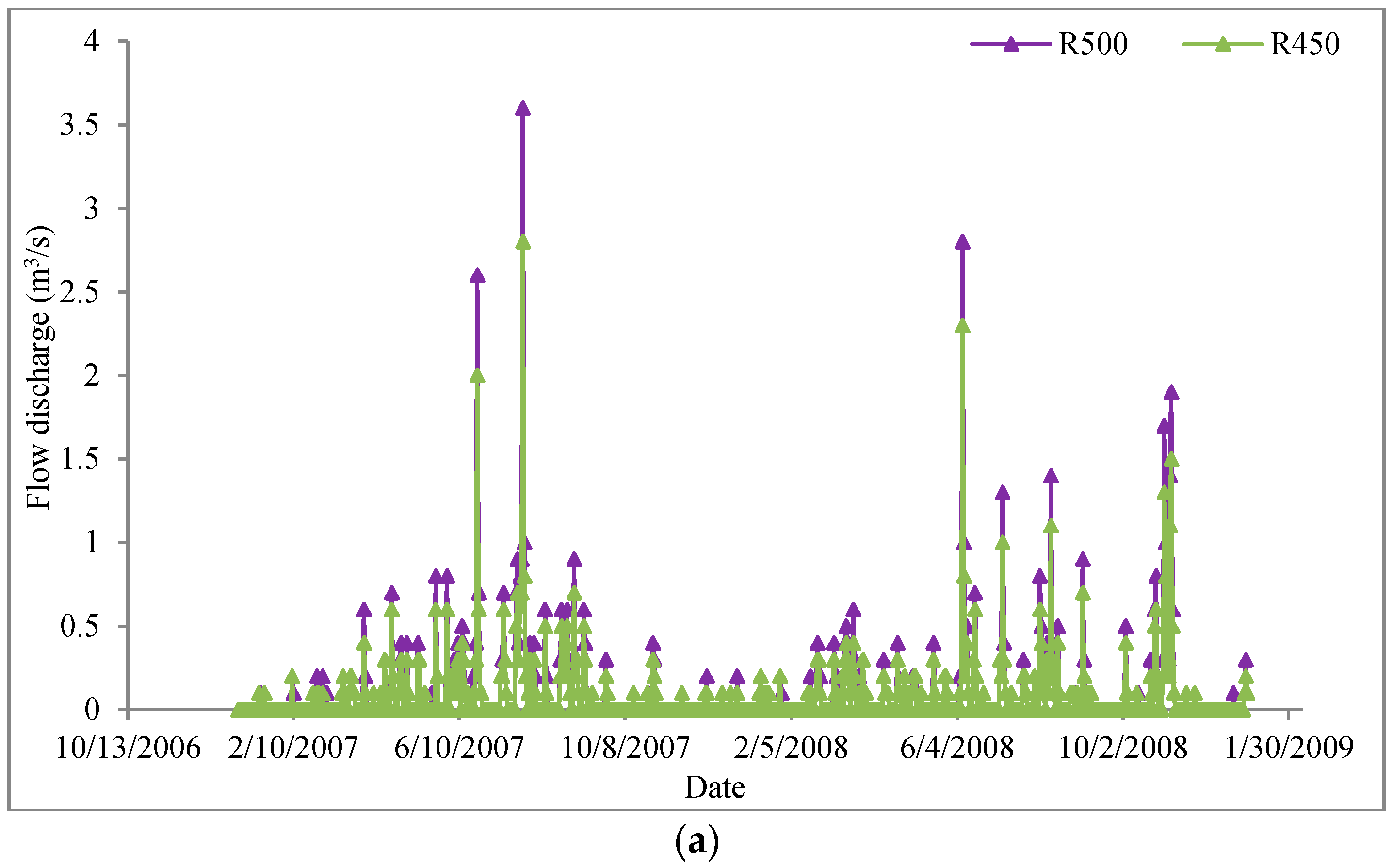
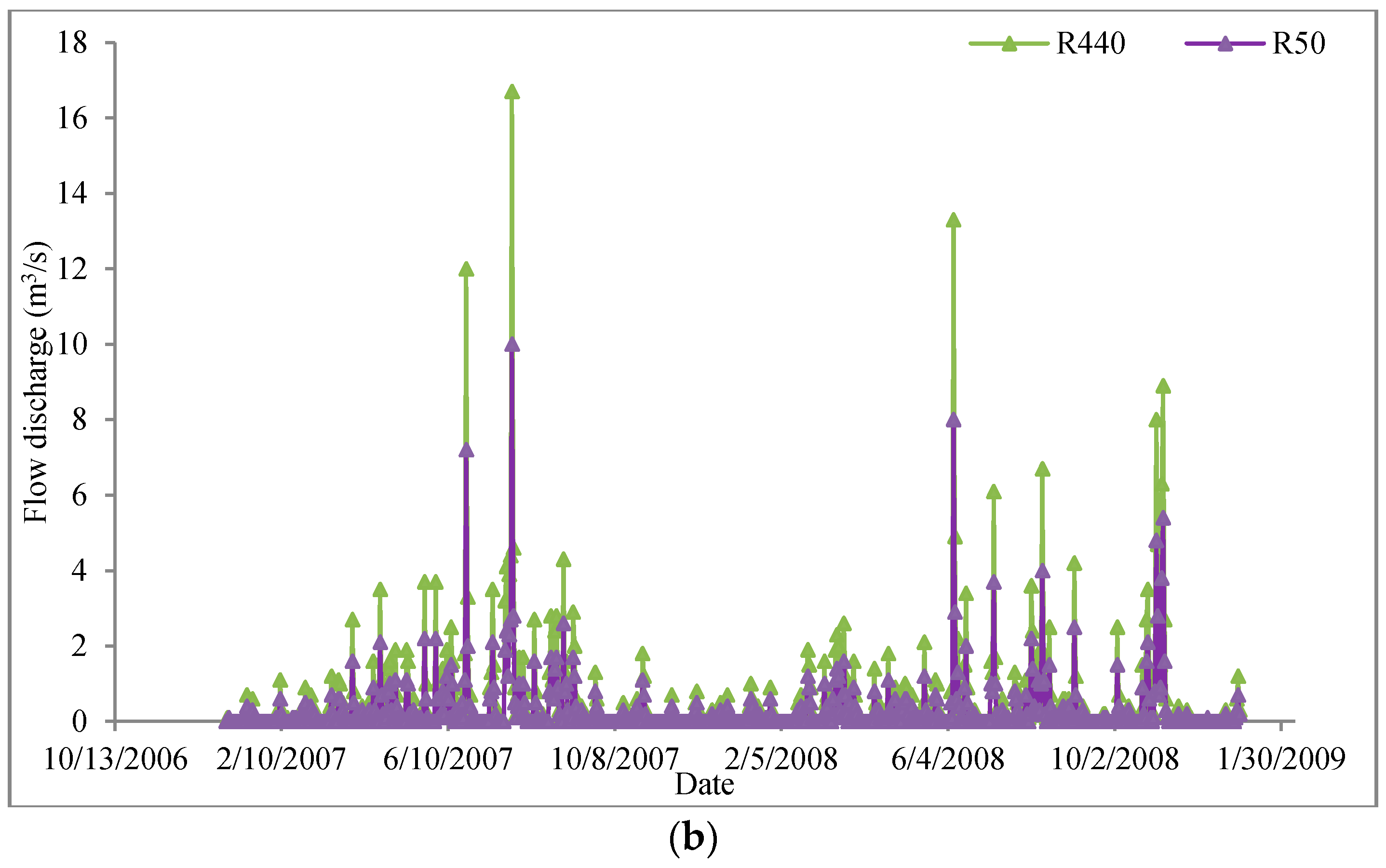
Figure 13.
Solids grading curves for the watercourse of Xiaxi River

Figure 14.
Comparison of W2 modeled and observed flow discharge.

Figure 15.
Comparison of W2 modeled and observed Hg concentrations: (a) THg, (b) DHg, (c) MeHg.

Table 1.
List of concentrations of Hg species computed in the W2 model.
| Symbol | Definition | Units |
|---|---|---|
| Hg0 | Hg0 concentration in water | ng·L−1 |
| HgII | Concentration of total HgII in water | ng·L−1 |
| HgIId | Concentration of dissolved HgII in water | ng·L−1 |
| HgIIdoc | Concentration of DOC adsorbed HgII in water | ng·L−1 |
| HgIIpom | Concentration of POM adsorbed HgII in water | ng·L−1 |
| HgIIpt | Total concentration of solids adsorbed HgII in water | ng·L−1 |
| HgIIpts | Total concentration of solids adsorbed HgII in water | ng·g−1 |
| HgII2 | Concentration of total HgII in sediment | ng·L−1 |
| HgIIdp2 | Concentration of dissolved HgII in pore water | ng·L−1 |
| HgIIdocp2 | Concentration of DOC adsorbed HgII in pore water | ng·L−1 |
| HgIIpom2 | Concentration of POM adsorbed HgII in sediment | ng·L−1 |
| HgIIpt2 | Total concentration of solids adsorbed HgII in sediment | ng·L−1 |
| HgIIpts2 | Total concentration of solids adsorbed HgII in sediment | ng·g−1 |
| MeHg | Concentration of total MeHg in water | ng·L−1 |
| MeHgd | Concentration of dissolved MeHg in water | ng·L−1 |
| MeHgdoc | Concentration of DOC adsorbed MeHg in water | ng·L−1 |
| MeHgpom | Concentration of POM adsorbed MeHg in water | ng·L−1 |
| MeHgpt | Total concentration of solids adsorbed MeHg in water | ng·L−1 |
| MeHgpts | Total concentration of solids adsorbed MeHg in water | ng·g−1 |
| MeHg2 | Concentration of total MeHg in sediment | ng·L−1 |
| MeHgdp2 | Concentration of dissolved MeHg in pore water | ng·L−1 |
| MeHgdocp2 | Concentration of DOC adsorbed MeHg in pore water | ng·L−1 |
| MeHgpom2 | Concentration of POM adsorbed MeHg in sediment | ng·L−1 |
| MeHgpt2 | Concentration of solids adsorbed MeHg in sediment | ng·L−1 |
| MeHgpts2 | Concentration of solids adsorbed MeHg in sediment | ng·g−1 |
Table 2.
Definition of symbols used in Equations (1)–(15).
| Symbol | Definition | Units |
|---|---|---|
| CL | cloud cover | / |
| DOC | dissolved organic carbon in water | mg·L−1 |
| DOC2 | dissolved organic carbon in pore water | mg·L−1 |
| fd | fraction of dissolved phase in water | / |
| fdoc | fraction of DOC adsorbed phase in water | / |
| fd2 | fraction of dissolved phase in sediment | / |
| fdoc2 | fraction of DOC adsorbed phase in sediment | / |
| fpom | fraction of POM adsorbed phase in water | / |
| Fpom2 | fraction of POM adsorbed phase in sediment | / |
| fpn | fraction of inorganic solid “n” adsorbed phase in water | / |
| fpn2 | fraction of inorganic solid “n” adsorbed phase in sediment | / |
| h | water depth | m |
| h2 | sediment layer thickness | m |
| Hg00 | air concentration of Hg0 | ng·L−1 |
| i | either HgII or MeHg | / |
| I0 | solar radiation at the water surface | W·m−2 |
| I0pht | light intensity when kpht is measured | W·m−2 |
| k12 | Hg0 oxidation rate in water | d−1 |
| kd21 | photoreduction rate of dissolved HgII in water | d−1 |
| kdoc21 | photoreduction rate of DOC adsorbed HgII in water | d−1 |
| kd23 | methylation rate of dissolved HgII in water | d−1 |
| kdoc23 | methylation rate of DOC adsorbed HgII in water | d−1 |
| kd31 | photolytic degradation rate of dissolved MeHg in water | d−1 |
| kdoc31 | photolytic degradation rate of DOC adsorbed MeHg in water | d−1 |
| kd32 | demethylation rate of dissolved MeHg in water | d−1 |
| kdoc32 | demethylation rate of DOC adsorbed MeHg in water | d−1 |
| kd32-2 | dissolved MeHg demethylation rate in sediment | d−1 |
| kso42 | sediment sulfate reduction rate | d−1 |
| KH | Henry’s law constant | Pa·m3·mol−1 |
| Kdoc | equilibrium partition coefficient for DOC in water | L·kg−1 |
| Kdoc2 | equilibrium partition coefficient for sediment DOC | L·kg−1 |
| Kpom | equilibrium partition coefficient for POM in water | L·kg−1 |
| Kpom2 | equilibrium partition coefficient for sediment POM | L·kg−1 |
| Kpn | equilibrium partition coefficient for inorganic solids in water | L·kg−1 |
| Kpn2 | equilibrium partition coefficient for sediment solids “n” | L·kg−1 |
| KSO4 | half-saturation constant for the effect of sulfate on methylation | mg-O2·L−1 |
| LHgII | atmospheric deposition rates of HgII | μg·m−2·d−1 |
| LMeHg | atmospheric deposition rates of MeHg | μg·m−2·d−1 |
| mn | inorganic solid “n” concentration in water | mg·L−1 |
| mn2 | inorganic solid “n” concentration in sediment | mg·L−1 |
| MeHg0 | air concentration of MeHg | ng·L−1 |
| POM | particulate organic matter in water | mg L−1 |
| POM2 | particulate organic matter in sediment | mg·L−1 |
| rmso4 | ratio of sediment methylation rate and sulfate reduction rate | L·mg−1 |
| R | universal gas constant | Pa·m3·mol−1·K−1 |
| SO42 | sediment pore water sulfate concentration | mg-O2·L−1 |
| SSHg0 | source/sink terms of Hg0 in water | μg·L−1·d−1 |
| SSHgII | source/sink terms of HgII in water | μg·L−1·d−1 |
| SSMeHg | source/sink terms of MeHg in water | μg·L−1·d−1 |
| SSHgII2 | source/sink terms of HgII in sediment | μg·L−1·d−1 |
| SSMeHg2 | source/sink terms of MeHg in sediment | μg·L−1·d−1 |
| Twk | water temperature | K |
| Y12 | Hg0 oxidation yield coefficient | g·g−1 |
| Y21 | HgII photoreduction yield coefficient | g·g−1 |
| Y23 | HgII methylation yield coefficient | g·g−1 |
| Y31 | MeHg photolytic degradation yield coefficient | g·g−1 |
| Y32 | MeHg demethylation yield coefficient | g·g−1 |
| ϕ | porosity | / |
| λmax | maximum light extinction coefficient | m−1 |
| vv-Hg0 | volatilization velocity of Hg0 | m·d−1 |
| vv-MeHg | volatilization velocity of MeHg | m·d−1 |
| vb | sediment burial velocity | m·d−1 |
| vpn | settling velocity of inorganic solid “n” | m·d−1 |
| vrn | sediment resuspension velocity of solid “n” | m·d−1 |
| vsom | settling velocity of POM | m·d−1 |
Table 3.
List of water quality parameters used in the test cases.
| Variable | Units | Value |
|---|---|---|
| Kp-HgII Kpom-HgII Kp-MeHg Kpom-MeHg | L·kg−1 L·kg−1 L·kg−1 L·kg−1 | 2.0 × 10³ (Silt and fine), 1.0 × 10³ (Sand) 1.0 × 10⁴ |
| 1.0 × 10³ (Silt and fine), 0.5 × 10³ (Sand) 0.5 × 10⁴ | ||
| KH-Hg0 | atm·m3·mol−1 | 0.0071 |
| vv-Hg0 | m·d−1 | 0.8 |
| Hg00 | ng·L−1 | 0.0 |
| k12 | d−1 | 0.001 |
| Y12 | g·g−1 | 1.0 |
| kd21 | d−1 | 0.01 |
| Y21 | g·g−1 | 1.0 |
| I0pht | W·m−2 | 100.0 |
| kd23 | d−1 | 0.002 |
| Y23 | g·g−1 | 1.07 |
| kd32 | d−1 | 0.04 |
| kd23_2 | d−1 | 0.01 |
| kd31 | d−1 | 0.01 |
| Y31 | g·g−1 | 0.93 |
| kd32_2 | d−1 | 0.005 |
| Y32 | g·g−1 | 0.93 |
Table 4.
Geometry of the Xiaxi River reaches and major tributaries.
| Reach Number | Reach Name | Length (m) | Slope | Remark |
|---|---|---|---|---|
| 1 | R450 | 646 | 0.17301 | Hg tailing |
| 2 | R500 | 2675 | 0.04434 | Hg tailing |
| 3 | R320 | 4687 | 0.02238 | Mainstem |
| 4 | R410 | 3388 | 0.02766 | Mainstem |
| 5 | R180 | 6813 | 0.01000 | Mainstem |
| 6 | R20 | 2017 | 0.01000 | Mainstem |
| 7 | R440 | 5688 | 0.03769 | Tributary |
| 8 | R50 | 7353 | 0.02745 | Tributary |
Table 5.
Comparison of modeled and observed TSS values.
| W2 model Segment No. | TSS (mg·L−1) | TSS (mg·L−1) | ||
|---|---|---|---|---|
| 4 September 2007 | 8 August 2008 | |||
| Modelled | Observed | Modelled | Observed | |
| 5 | 1.75 | 1.7 | 4.26 | 4.4 |
| 22 | 0.7 | 0.76 | 1.95 | 2 |
| 36 | 0.55 | 0.44 | 2.15 | 2.2 |
| 51 | 0.55 | 0.7 | 2.14 | 2.1 |
Table 6.
Relative errors (%) of modeled DHg with different values of Kd (L·kg−1).
| Kd for Fine Solids/Kd for Coarse Solids | 102 | 103 | 104 | 105 | 106 |
|---|---|---|---|---|---|
| 104 | 33.47 | 30.95 | 29.54 | 29.26 | 32.79 |
| 105 | 29.16 | 26.30 | 24.68 | 24.37 | 27.97 |
| 106 | 18.53 | 14.23 | 11.75 | 12.29 | 15.42 |
| 107 | 39.06 | 35.03 | 32.67 | 32.20 | 38.84 |
Table 7.
Relative errors (%) of modeled MeHg with different M/D rates (d−1).
| M/D | 10−2 | 10−1 | 1 |
|---|---|---|---|
| 10−1 | 15.98 | 28.45 | 25.06 |
| 10−2 | 11.81 | 9.93 | 13.37 |
| 10−3 | 12.20 | 14.14 | 19.53 |
| 10−4 | 12.69 | 14.65 | 20.18 |
| 10−5 | 14.27 | 16.10 | 20.24 |
© 2017 by the authors. Licensee MDPI, Basel, Switzerland. This article is an open access article distributed under the terms and conditions of the Creative Commons Attribution (CC BY) license (http://creativecommons.org/licenses/by/4.0/).
Share and Cite
MDPI and ACS Style
Zhu, S.; Zhang, Z.; Liu, X. Enhanced Two Dimensional Hydrodynamic and Water Quality Model (CE-QUAL-W2) for Simulating Mercury Transport and Cycling in Water Bodies. Water 2017, 9, 643. https://doi.org/10.3390/w9090643
AMA Style
Zhu S, Zhang Z, Liu X. Enhanced Two Dimensional Hydrodynamic and Water Quality Model (CE-QUAL-W2) for Simulating Mercury Transport and Cycling in Water Bodies. Water. 2017; 9(9):643. https://doi.org/10.3390/w9090643
Chicago/Turabian StyleZhu, Senlin, Zhonglong Zhang, and Xiaobo Liu. 2017. "Enhanced Two Dimensional Hydrodynamic and Water Quality Model (CE-QUAL-W2) for Simulating Mercury Transport and Cycling in Water Bodies" Water 9, no. 9: 643. https://doi.org/10.3390/w9090643
Note that from the first issue of 2016, this journal uses article numbers instead of page numbers. See further details here.