Integrating Topography and Soil Properties for Spatial Soil Moisture Storage Modeling


1
College of Hydrology and Water Resources, Hohai University, Nanjing 210098, China
2
State Key Laboratory of Hydrology-Water Resources and Hydraulic Engineering, Hohai University, Nanjing 210098, China
3
School of Civil Engineering and Environmental Sciences, University of Oklahoma, Norman, OK 73019, USA
4
Advanced Radar Research Center, National Weather Center, Norman, OK 73019, USA
*
Author to whom correspondence should be addressed.
Water 2017, 9(9), 647; https://doi.org/10.3390/w9090647
Submission received: 14 July 2017
/
Revised: 15 August 2017
/
Accepted: 24 August 2017
/
Published: 30 August 2017
(This article belongs to the Special Issue Soil Water Conservation: Dynamics and Impact)
Abstract
:The understanding of the temporal and spatial dynamics of soil moisture and hydraulic property of soil is crucial to the study of hydrological and ecological processes. The purpose of this study was to derive equations that describe spatial soil water storage deficit based on topography and soil properties. This storage deficit together with the topographical index can be used to conclude the spatial distribution curve of storage capacity in a (sub-) basin for developing hydrological model. The established model was able to match spatial and temporal variations of water balance components (i.e., soil moisture content (SMC), evapotranspiration, and runoff) over the Ziluoshan basin. Explicit expression of the soil moisture storage capacity (SMSC) in the model reduced parameters, which provides a method for hydrological simulation in ungauged basins.
1. Introduction
The understanding of the temporal and spatial dynamics of soil moisture and hydraulic property is crucial to the study of several hydrological and ecological processes. Soil moisture is a key variable in hydrological modeling. As McNamara et al. [1] pointed out that understanding soil storage and its role in regulating catchment functions should be a priority in future observation strategies and hydrological modelling. Soil moisture and hydrological routing is computed based on the saturated and unsaturated flow equations, which can be solved by finite element or difference techniques over a three dimensional grid. These models include System Hydrological European model (SHE) [2,3] and Institute of Hydrology Distributed Model (IHDM) [4,5]. While the advantages of pure, numerical simulation would seem clear, the tremendous amount of parameter evaluation required is problematic. In most cases the available data motivates the use of simple, conceptual model approaches rather than the use of a fully distributed, physically model with a large number of model parameters [6].
It is widely recognized that for saturation excess overland flow, soil storage is one of the key elements controlling runoff production in catchments in humid temperate areas. For traditionally lumped hydrological models, soil moisture is usually computed on the basis of basin average routing of unsaturated water balance, and its spatial variation is expressed in an empirical distribution curve of soil moisture storage capacity, e.g., a single parabolic curve in Xin’anjiang hydrological model [7]. The model usually lacks physical expressions and distribution functions of the hydrological processes or parameters, which solely calibrated based on observed flow discharge.
The semi-distributed models are capable to overcome shortage of the empirical models since they explicitly express watershed distribution of soil moisture storage using site-specific information of land surface features, e.g., soil properties and topography. For example, the topographic index [8] is widely used to analytically describe such distribution of soil moisture and runoff generation [9]. It is also used for improving the empirical hydrological models with a distributed function. Such as the Xin’anjiang model, the statistical curve of spatial distribution of storage capacity was directly derived from TOPMODEL’s topographic index [10,11,12] and from catchment slopes [13] or the empirical shape parameter B of the water storage capacity of the soil non-linearly was estimated in terms of the characteristic land surface slope [14]. Some signal from the topography and soil type was used to explain the soil moisture variation [15]. These models are benefit from a combination of reasonable computation time and physically realistic hillslope simulation.
Explicitly description of storage capacity for computation of hydrological fluxes remains challenge as it relates to topography, soil, vegetation and base rock variations. In the mountainous areas, topography controls depth to groundwater table and thus distribution of soil moisture deficit. In the hilly lowland areas, near stream saturated zones will be most extensive in locations with concave hillslope profiles and wide flat valleys (Figure 1). The storage deficit in the unsaturated zone becomes small and the runoff is easily generated because the unsaturated zone for holding soil moisture is reduced due to the high groundwater table occupation or low active depth of the unsaturated zone [12].
The available space for moisture storage in unsaturated zone depends on not only the active depth but also the rise of the capillary fringe (Figure 1). Surface tension and soil pore capillary force lead the groundwater rise up into the soil and form a capillary fringe with a certain thickness [16], which significantly decreases soil moisture deficit. The capillary rise is associated with physical properties of soil porosity and particle diameter. For clay, where capillary is strong, a water table depth of 10 m can still be “felt” in the root zone and near surface. For sand, the water table has little role as a source if it is below the root zone [17]. It is found that low runoff potential for soils having the low rise of the capillary fringe, such as deep sand, deep loess, aggregated silts, and high runoff potential for soils having the high rise of the capillary fringe, such as heavy plastic clays, and certain saline soils [18].
The main objective of this study is to derive equations for description of the spatial soil storage capacity that can make use of topography and soil property in the humid hilly watershed. The equations were derived by combining the van Genuchten model of water retention relationship [19] and the TOPMODEL topographic index. They can be used to describe the site specific soil storage capacity and its statistical feature in a (sub-) basin, thus to simulate spatial distribution of hydrological variables of runoff amount, evaporation and soil water storage. The model was tested on Ziluoshan basin of Huai River watershed in the humid region in China.
2. Materials and Methods
2.1. Description of Ziluoshan Basin
As one of the first tributaries in the upstream of Huai River, Shaying River originated in the western mountainous area of Henan province of China (Figure 2). The watershed area above the Ziluoshan hydrological station on Shaying River is 1800 km2, and the mountainous area accounts for 75%. These geographical and climatic features result in extremely uneven of the annual and seasonal distributions of rainfall. The annual precipitation during 1980–1996 is 900 mm, varying from the largest in the southeast to the smallest in the north. Most of annual precipitation is concentrated in the flood seasons (June–September). Nearly 60–70% of the total precipitation occurs in the months of June and August.
DEM data of 30 m grid resolution are used to describe the spatial variations of topography [20,21]. Based on the geographical map, the terrain of the catchment tilts from southwest to northeast (Figure 2). The mean elevation of topography is 820 m, varying from 284 m above the mean sea level in the downstream region to over 2122 m in the upstream mountainous areas. The topographic index in each pixel was calculated using the DTM9704 program [22,23].
Soil in the basin is primarily shallow eluvial-slope deposits consisting of sand, loam and clay (Data Center for Resources and Environmental Sciences Chinese Academy of Sciences (RESDC)). Percentage of sand and clay within the soil depth of 0–1.0 m ranges 5.3–83.0% for sand, 1.7–31.6% for clay (Figure 3), and the remaining for loam. Value of the hydraulic parameters for the three soils refers to Tuller [24] (Table 1). The mean values of soil hydraulic parameters of VG in each pixel were estimated by proportion-weighted arithmetic mean way, and the field capacity θf was determined as a fraction of the saturated SMC (75% in this study [25]). The vegetation in the study region is primarily deciduous broadleaf forest and mixed forest. The average vegetation coverage is larger than 75% [26] and average annual Normalized Difference Vegetation Index (NDVI) is larger than 0.6 [27].
The watershed was divided into a number of sub-basins (e.g., 50 sub-basins in this study) for describing spatial variations of runoff generation and river flow routing (Figure 4). Each sub-basin includes lots of pixels in 30 m grid resolution.
2.2. Outline of the Model
The soil moisture storage model was firstly introduced at site scale, and then extended to hillslope soil moisture storage capacity (SMSC) according to TOPMODEL concept. Finally, a spatial soil moisture storage curve was concluded by all sites SMSC in a statistical way to replace the traditional statistical curve in Xin’anjiang model. The detail procedure is given blow.
2.2.1. The Role of Soil Moisture Storage on Hydrological Fluxes
Hydrological balance on any element can be expressed as following:
where and is soil moisture storage at the time interval of t − 1 and t, Pt, Et and Rt is precipitation, actual evapotranspiration and runoff at the time interval of t − 1 and t, respectively.
In Equation (1), computation of both actual evapotranspiration E and runoff R depends on soil storage W (SMC in this model) and its capacity Wm (SMSC in this model), e.g., for saturation excess overland flow, runoff is generated as the soil storage reaches the capacity, which can be expressed as following:
where Pe is net rainfall.
For distributed modeling or physical description of spatial variation function of watershed characteristics on hydrological fluxes, expression of soil spatial variation storage and its capacity in a watershed is vital.
2.2.2. Site Specific Soil Moisture Storage Capacity
SMSC is usually defined as the difference between the water content at field capacity and at residual multiplied by a critical depth in unsaturated zone for moisture storage and runoff generation. In humid regions, the critical depth can be regarded as unsaturated zone thickness or the depth to free water table if there is a free water table in the soil profile. In this case, vertical water content in the critical depth can be influenced by the free water table under the capillary flux from the free water to soil moisture column (Figure 1a), which results in that soil moisture seldom reach the residual water content on the groundwater table nearby. Thus, the soil moisture profile above the water table can be determined from the balance between the pressure head gradient, which tends to draw moisture up, and gravity [28].
The soil-water pressure head distribution, , may be modeled using Darcy’s law:
or
where q is the steady state evaporation rate, is the unsaturated hydraulic conductivity function, is the pressure head (m).
Soil moisture with depth can be described by the van Genuchten model (hereafter VG) of water retention relationship [19,29]:
where is the pressure head (m), θs and θr is saturated and residual volume water contents, respectively, α, n are fitting parameters.
Solution of Equation (3) or Equation (4) coupling with Equation (5) is a rather complicated although analytical steady state solutions can be found in the literature for some functions different with VG [30,31]. These mathematical difficulties are significantly reduced if the vertical profile of soil moisture is approximated with the profile corresponding to zero-flux conditions [32]. Under the assumption of zero vertical flux (quasi steady-state hydraulic assumption), the relationship between and vertical distance above groundwater table (z is taken here to increase upwards) is that of hydraulic equilibrium:
where D is the depth to groundwater table.
Some comparisons between the vertical profile of soil moisture obtained with Equation (3) and the approximated profile provided by Equation (6) have been made in many literatures. It was found that difference of the soil moisture profiles between the two equations increases when the depth z increases to the nearby surface and the soil texture becomes finer. However, the difference between the two profiles is smaller than 5–7% for a variety of soil textures [33]. For shallow water tables, the steady profile is close to hydrostatic state subject to no atmospheric forcing [34].
For the steady profile, the total profile moisture deficit will be obtained by integrating from the surface to the top of the capillary fringe. Using Equations (5) and (6), we obtain a simple mathematical expression for the unsaturated zone moisture storage Sf(D), given the depth to groundwater table D:
where is suction pressure for the unsaturated zone storage at field capacity.
Hence, the soil moisture deficit or SMSC Wm(D) defined as the difference between the moisture content at field capacity θf and at the unsaturated zone moisture profile Sf(D) in Equation (7) is given by:
Equation (8) explicitly expresses the storage capacity in terms of the site specific depth to groundwater table and hydraulic parameters of soil. A large storage capacity corresponds to low groundwater table and low capillary fringe.
2.2.3. Hillslope SMSC
In a hilly mountain area, the topographic index is widely used to represent the influences of terrain on the spatial variations of soil wetness. In TOPMODEL, the large topographic index always being obtained in the local valley area, where happened to be the saturated zone. So a larger topographic index in a local area means less soil moisture deficit or easier runoff generation in response to rainfall input [12]. Figure 1b illustrates that the local moisture deficit varies significantly along the catchment slope, with low values where the water table is near the surface (at the bottom of hills) and high values where the water table is deeper (at the top of hills) [35].
According to TOPMODEL concept, the depth to groundwater table at any location is given in terms of the watershed average depth to the water table and local topography wetness index [8]:
where Di is the depth to groundwater table at the location i, is the watershed-average depth to the water table, Szm is a scaling parameter, known as the ‘effective depth’ that determines the decay of hydraulic conductivity with depth, tpi is local topography wetness index (, where a is the cumulative area draining through a unit length of contour line, β is the slope of the unit area), is the areal average of tpi.
Equation (9) is written in the form:
Equation (10) is substituted into Equation (8) to get:
Equation (11) explicitly expresses soil moisture deficit at any location influenced by integration of soil properties, topography and depth to groundwater table.
The local storage capacity Wm(Di) and its basin mean value WM solely depend on the effective soil depth Szm if other parameters in the van Genuchten model in Equation (11) are measured or given according to available investigations. Beven et al. [36] described that larger value of the parameter Szm means increase of active soil depth for water storage and runoff generation. Habets and Saulnier [37] stated that the parameter Szm can be defined as one quarter of the maximum storage deficit.
In some humid area like Ziluoshan basin, streams are typically gaining streams (gaining water by drainage of baseflow from the groundwater into the stream). For the perennial rivers, the groundwater table near the surface is coincident or close to the stream water surface elevation [18,38]. Thus Di and Wm(Di) approach zero in the areas nearby the stream water surface where tpi reaches its maximum value. Then, coefficient C in Equation (10) is:
Equation (12) is substituted into Equation (11) to get:
2.2.4. The Watershed Model Development
The model can be executed at each grid based on storage capacity Wm(Di) at any local area calculated in terms of Equation (11). For runoff generation, grid runoff depth for a specific precipitation amount can be calculated based on saturation overland flow concept that runoff occurs where soil moisture reaches storage capacity (Equation (2)).
The site-specific storage capacity can be grouped into a number of intervals, each representing that fraction of the watershed with similar water table depth and soil moisture characteristics [39]. Water balance equations (Equation (2)) are applied at each interval, which separate estimates of unsaturated zone soil moisture, evapotranspiration and runoff for the whole intervals [40,41,42]. The individual fluxes in every interval are then really weighted and combined to obtain the water balance for the entire watershed. This modeling method is efficient in computation of flow routing and parameter calibration of the model.
For a large watershed, the model can be executed at each sub-basin based on distribution curve of Wm ~ f/F (f/F represents proportion of Wm value in a specific interval with an area f to the total (sub-) basin area F, the ratio value is between 0 and 1.) and its average value WM in a (sub-) basin. This modeling method becomes lumped structure like Xin’anjiang model, but it physically interprets the field capacity curve that allows for application in ungauged basins and consecutive routing in the large watershed.
Computations of actual evaporation, separation of runoff components and flow routing in the watershed and rivers are same as Xin’anjiang model in this study. The calibrated parameter meaning was listed in Table 2. A spatial distribution curve of free water storage capacity with a catchment average SM and an exponent of the spatial distribution curve, EX, is used to represent regulation of catchment heterogeneity on free water R. For thin soils, SM is around 10 mm, and EX is between 1.0 and 1.5 [43]. The free water R is then separated into overland flow Rs, subsurface flow Ri, and deep layer flow (groundwater) Rg. KI and KG are the outflow coefficients of the free water storage to interflow and groundwater. It is suggested that the sum KI + KG may be taken as 0.7–0.8 and the ratio of the three runoff components will be changed by altering the ratio of KG/KI [43].
For application of the model in a large watershed, the whole watershed can be divided into a lot of sub-basins. These sub-basins are linked with the river channel system. The flow hydrograph at a point on the watershed from a known hydrograph of upstream or sub-basin is routed by the Muskingum method. Small tributaries of sub-basins merge to form larger stream which ultimately lead to outlet of the watershed.
2.3. Model Verification
Within the study area, daily and hourly observed precipitation data at 7 rainfall stations, pan evaporation and streamflow at the outlet of watershed were used for model testing (Figure 2). The largest and smallest streamflow discharges during 1979 and 1995 are 2080.0 and 1.0 m3/s, respectively. Daily and hourly rainfall in each of the watershed was interpolated by the thiessen polygon method from observation data of rainfall stations. The model is calibrated and validated based on daily and hourly observed streamflow discharges at the whole watershed outlet in calibration and validation periods, respectively. The calibration period is 10 years from 1979 to 1988, and the validation period is 7 years from 1989 to 1995. Twelve and seven flood events with hourly observation data in calibration and validation periods, respectively, are further selected for model calibration and validation.
The calibration procedures followed the Xin’anjiang model calibration proposed by Zhao et al. [43]: (1) giving initial values of the parameters suggested; (2) calibrating the parameters of runoff generation processes to test annual water balance, e.g., KC in Table 2, by comparing totals of the simulated and observed runoff; (3) calibrating other parameters of water source separation and flow routing in Table 2 to test flow discharges by comparing the simulated and observed runoff. Model performance is evaluated with respect to the objective function of maximizing Nash–Sutcliffe efficiency coefficient (NSC) between observed and simulated runoff. Another measure of model performance used in the study is the root mean squared error (RMSE) of flow discharge. The calibrated parameters and values were listed in Table 2. The calibrated value of Szm is 42.8 mm. It is used to calculate mean value of storage capacity WM in each sub-basin and in whole watershed. The sub-basin mean WM for the 50 sub-basins ranges 107–127 mm, and whole watershed WM is 120 mm.
3. Result and Discussion
The calibration and validation results of flow discharges for daily and hourly data are listed in Table 3 and Table 4, respectively. For daily simulation during the calibration period (Table 3), mean NSC value is 0.73, annually ranging 0.47–0.91; mean RMSE is 1.6 mm, annually ranging 0.6–4.4 mm. The daily simulation results during the validation period are even better than those in the calibration period, e.g., mean NSC value is 0.77, ranging 0.67–0.87; mean RMSE is 1.0 mm, ranging 0.6–1.4 mm.
The model captured the flood processes (Table 4 and Figure 5) as well. During the calibration and validation periods, respectively, mean NSC value of all flood events is 0.85 and 0.83; the relative error of the simulated and observed peak discharges is 3.70% and 2.26%; mean RMSE is 44.5 and 35.6 m3/s. For illustrative purpose, hourly simulated and observed flood discharges are shown in Figure 5. These results demonstrated that the model is capable of reproducing both the magnitude and the dynamics of the daily and hourly flow discharges.
3.1. Sensitivity Analysis
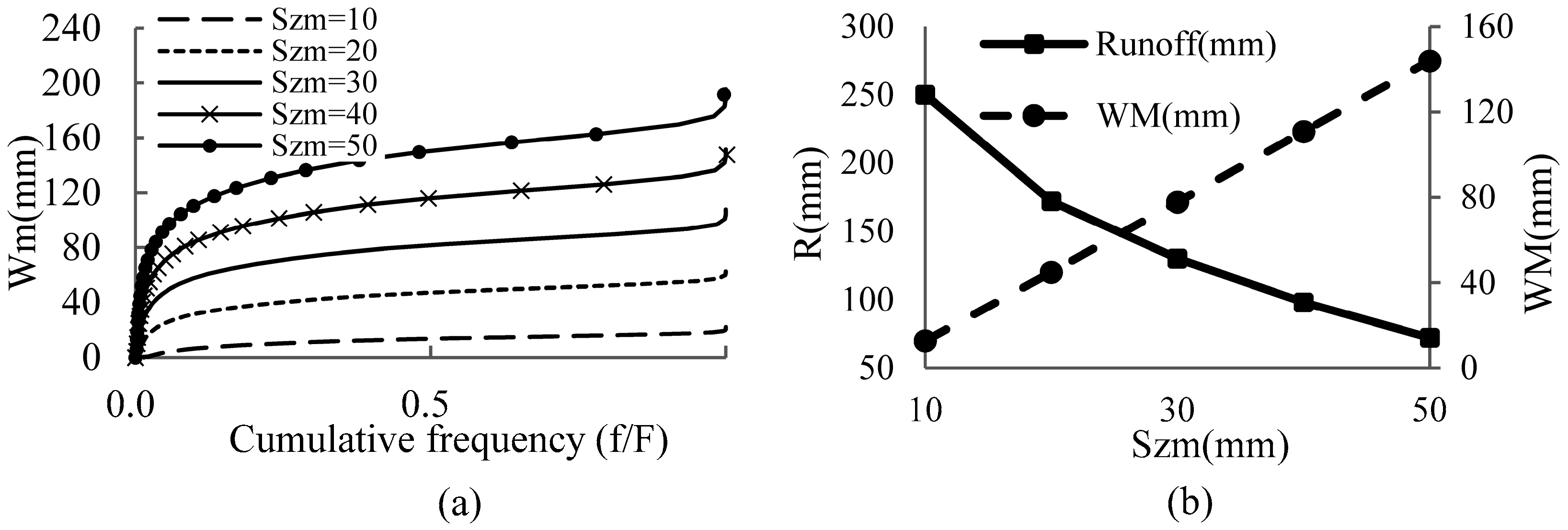
In this study, sensitivity analysis of parameters for the effective depth Szm and soil properties was carried out to evaluate and quantify the effect of the parameter variations on model output. Curves of Wm ~ f/F for Szm values within 10–50 mm in the whole watershed were shown in Figure 6a. Sensitive analysis was executed by simulating changes of streamflow in response to these curves. For the specific soil distribution in the study watershed (Figure 3), change of mean annual streamflow for the flood period 11 May–23 September 1985 responded to changes in Szm and WM are shown in Figure 6b. Increase of Szm significantly increased WM and thus decreased runoff. Simulated results indicate that as Szm increased from 10 to 50 mm, WM increased from 12.6 to 143.8 mm, resulting in 70.0% decrease of runoff from 251.5 to 75.4 mm.
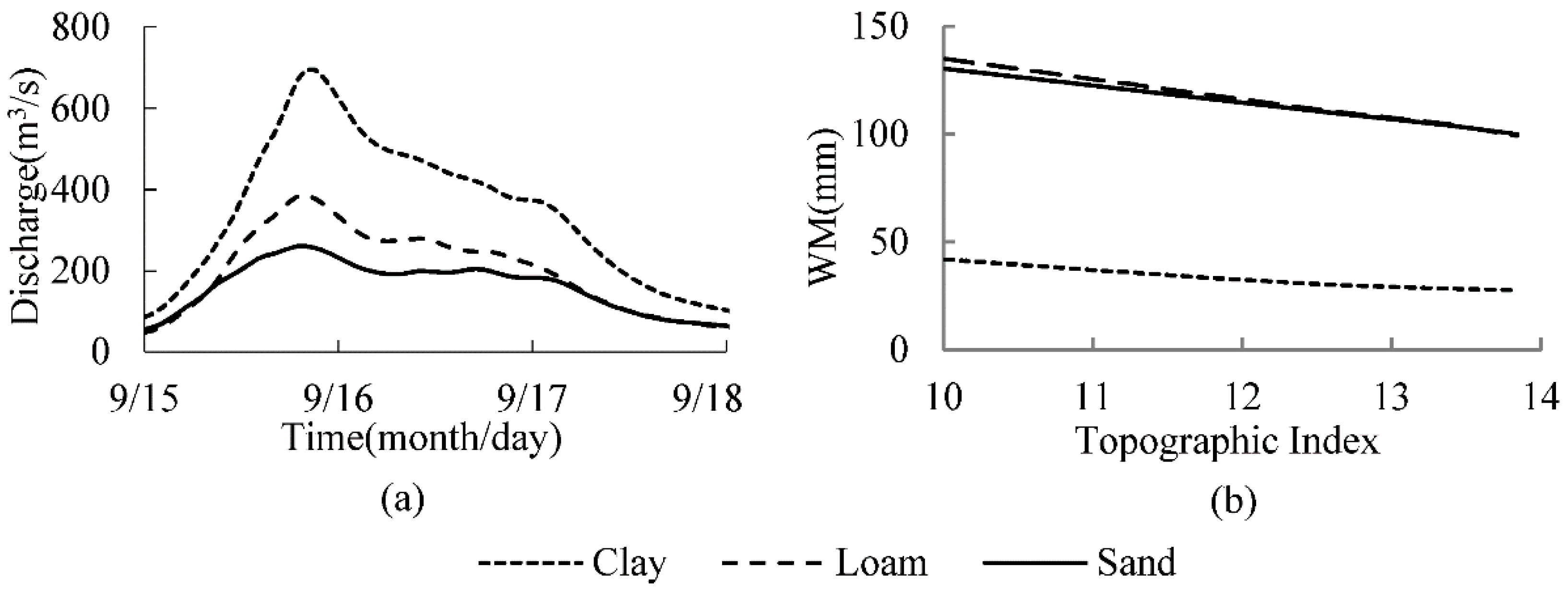
Sensitivity of soil properties on model output was executed for the rainfall. If the soils in the whole watershed were replaced by one of the three soils (silt, sandy loam and clay), the analysis results of relationship between WM and topographic index in 50 sub-basins indicated that sub-basin mean WM decreased with the topographic index increase (Figure 7a). Because of high residual moisture content θr and capillary rise for clay, the storage capacity WM for clay was much smaller than that of sand and sandy loam. Therefore, precipitation on the clay soil generates much more runoff than that on sand and sandy loam. As an example, simulated flood discharges for the precipitation of 81.9 mm during 15–18 September 1985 for sand, sandy loam and clay are shown in Figure 7b. This amount of precipitation generates runoff of 55.8 mm for clay, 42% and 52% larger than the generated runoff of 32.4 and 26.6 mm for sandy loam and sand, respectively. For the simulated flood events, the peak discharge generated on clay is 696.0 m3/s, 44% and 63% larger than the peak discharges of 386.0 and 260.0 m3/s on sandy loam and sand, respectively.
3.2. Spatial Variation of Hydrological Components
For hydrological modeling, distribution of the three components, soil moisture content, actual evapotranspiration and runoff, are vital for water resources management, environmental protection and assessment of land use and climate change impacts on hydrology. A major strength of the model is its capability to describe the spatial variations of such components.
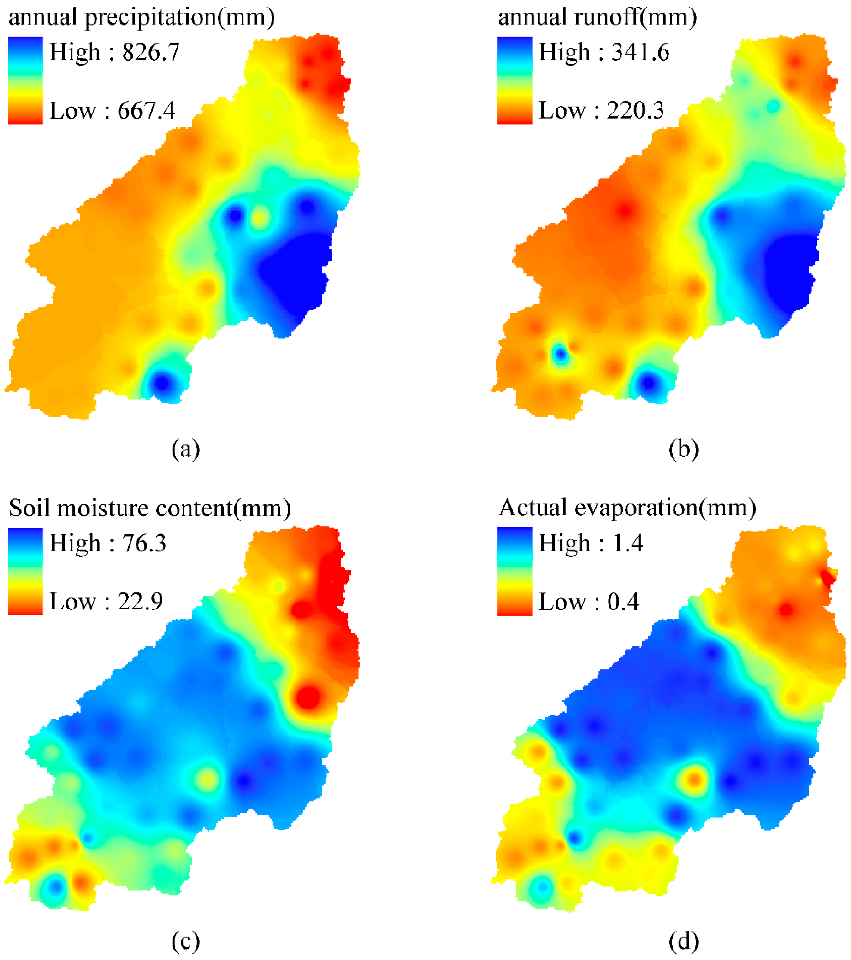
The developed model was executed in each of sub-basins with rainfall input and Wm ~ f/F curves (Figure 4). The hydrological components, i.e., soil moisture content, actual evapotranspiration and runoff were calculated in each sub-basin and their spatial variations were then described. For illustrative purposes, spatial variations of mean annual precipitation and runoff during 1980–1996 simulated by the model are shown in Figure 8a,b and soil moisture content and actual evapotranspiration on 1 October 1987 after a non-rainfall period of 20 days are shown in Figure 8c,d.
Figure 8 demonstrates that for the multi-year average, runoff distribution (Figure 8b) agrees with precipitation distribution (Figure 8a), larger in south and southwest of the high mountain area and smaller in the north and north east. Simulated results in Figure 8a and Figure 8b indicate that actual evaporation distribution generally corresponds to soil moisture content distribution, and both components are controlled by storage capacity for a specific time. As shown in Figure 8c, soil moisture content on 1 October 1987 is larger in the middle areas of watershed with a high value of WM (mostly higher than 120 mm in Figure 4b), and smaller in the north and south areas of the watershed with a low value of WM (mostly lower than 120 mm in Figure 4b). Larger soil moisture offers more water for evaporation (Figure 8d).
4. Conclusions
For the saturation excess overland flow modeling, the critical spatial soil moisture distribution was usually represented either by a grid by grid method or a distribution curve based on the controlling component, such as soil moisture (deficit). The latter method was generally more efficient, but such curve was traditionally empirical and lacked of directly physical interpretation, which did not allow for the extended application in ungauged basins. In order to overcome the limitations, the storage capacity distribution curve in a (sub-) basin was explicitly expressed by the van Genuchten model and topographic index in TOPMODEL on the basis of digital elevation and soil map. Because the new model had capacity in describing soil moisture deficit at a grid scale or its statistical curve in a sub-basin, the model could be used to simulate temporal and spatial distributions of hydrological components, and to investigate their relation with precipitation, topography and soil variations.
The model had been proven to be a reliable and flexible tool for rainfall-runoff modelling in Ziluoshan basin. The results demonstrated that the model was not only capable of reproducing daily and hourly flow discharges, but also able to produce reasonable spatial variations of hydrological components such as runoff, soil moisture storage and actual evapotranspiration. Sensitivity analysis showed effect of the soil effective depth and soil properties on runoff. This study helped us to understand scale effects of land surface characteristics on hydrological processes.
Acknowledgments
This research is supported by the National Key R&D Programme of China (No. 2016YFA0601000) and the Fundamental Research Funds for the Central Universities (Grant No. 2015B20314).
Author Contributions
Xiaohua Xiang contributed to the experiment design; Xiaoling Wu contributed to the data analysis and manuscript review; Xi Chen contributed to the experiment design, manuscript preparation and editing; Qifeng Song contributed to the data analysis and manuscript review; Xianwu Xue contributed to the manuscript review.
Conflicts of Interest
The authors declare no conflict of interest.
References
- McNamara, J.P.; Tetzlaff, D.; Bishop, K.; Soulsby, C.; Seyfried, M.; Peters, N.E.; Aulenbach, B.T.; Hooper, R. Storage as a metric of catchment comparison. Hydrol. Process. 2011, 25, 3364–3371. [Google Scholar] [CrossRef]
- Abbott, M.B.; Bathurst, J.C.; Cunge, J.A.; O’Connell, P.E.; Rasmussen, J. An introduction to the European Hydrological System-Systeme Hydrologique Europeen, SHE. 1. History and philosophy of a physically-based distributed modelling system. J. Hydrol. 1986, 87, 45–59. [Google Scholar] [CrossRef]
- Abbott, M.B.; Bathurst, J.C.; Cunge, J.A.; O’Connell, P.E.; Rasmussen, J. An introduction to the European Hydrological System-Systeme Hydrologique Europeen, SHE. 2 Structure of a physicallybased distributed modelling system. J. Hydrol. 1986, 87, 61–77. [Google Scholar] [CrossRef]
- Beven, K.J.; Calver, A.; Morris, E.M. The Institute of Hydrology Distributed Model; Report 98; The Institute of Hydrology: Wallingford, UK, 1987. [Google Scholar]
- Binley, A.; Elgy, J.; Beven, K.J. A physically based model of heterogeneous hillslopes: 1. Runoff Production. Water Resour. Res. 1989, 25, 1219–1226. [Google Scholar] [CrossRef]
- Seibert, J.; Bishop, K.; Rodhe, A.; McDonnell, J.J. Groundwater dynamics along a hillslope: A test of the steady state hypothesis. Water Resour. Res. 2003, 39, 1014. [Google Scholar] [CrossRef]
- Zhao, R.J.; Zhuang, Y.L.; Fang, L.R.; Liu, X.R.; Zhang, Q.S. The Xin’anjiang model. In Hydrological Forecasting; IAHS Publication No. 129; IAHS Press: Wallingford, UK, 1980; pp. 351–356. [Google Scholar]
- Beven, K.J.; Kirkby, M.J. A physically based variable contributing area model of basin hydrology. Hydrol. Sci. Bull. 1979, 24, 43–69. [Google Scholar] [CrossRef]
- Pellenq, J.; Kalma, J.; Boulet, G.; Saulnier, G.M.; Wooldridge, S.; Kerr, Y.; Chehbouni, A. A disaggregation scheme for soil moisture based on topography and s O’Kane oil depth. J. Hydrol. 2003, 276, 112–127. [Google Scholar] [CrossRef]
- Bell, V.A.; Moore, R.J. A grid-based distributed flood forecasting model for use with weather radar data: Part 1. Hydrol. Earth Syst. Sci. 1998, 2, 265–281. [Google Scholar] [CrossRef]
- Guo, F.; Liu, X.R.; Ren, L.L. Topography based watershed hydrological model-TOPOMODEL and its application. Adv. Water Resour. 2000, 11, 296–301. (In Chinese) [Google Scholar]
- Chen, X.; Chen, Y.D.; Xu, C.Y. A distributed monthly hydrological model for integrating spatial variations of basin topography and rainfall. Hydrol. Process. 2007, 21, 242–252. [Google Scholar] [CrossRef]
- Kong, F.Z.; Song, X.M. A Computation Method for Spatial Distribution of Soil Moisture Storage Capacity in Xin’anjiang Model. J. China Hydrol. 2011, 31, 1–14. (In Chinese) [Google Scholar]
- Dumenil, L.; Todini, E. A rainfall-runoff scheme for use in the Hamburg climate model. In Advances in Theoretical Hydrology, A Tribute to James Dooge; O’Kane, J.P., Ed.; Elsevier Science Publishers B.V.: Amsterdam, The Netherlands, 1992; pp. 129–157. [Google Scholar]
- Blyth, E.M.; Finch, J.; Robinson, M.; Rosier, P. Can soi1 moisture be mapped onto the terrain? Hydrol. Earth Syst. Sci. 2004, 8, 923–930. [Google Scholar] [CrossRef]
- Carman, P.C. Capillary rise and capillary movement of moisture in fine sans. Soil Sci. 1941, 52, 1–14. [Google Scholar] [CrossRef]
- Fan, Y.; Miguez-Macho, G.; Weaver, C.P.; Walko, R.; Robock, A. Incorporating water table dynamics in climate modeling: 1. Water table observations and equilibrium water table simulations. J. Geophys. Res. 2007, 112, D10125. [Google Scholar] [CrossRef]
- Todini, E. The ARNO rainfall-runoff model. J. Hydrol. 1996, 175, 339–382. [Google Scholar] [CrossRef]
- Van Genuchten, M.Th. A closed-form equation for predicting the hydraulic conductivity of unsaturated soils. Soil Sci. Soc. Am. J. 1980, 44, 892–898. [Google Scholar] [CrossRef]
- ASTER GDEM Readme File-ASTER GDEM Version1. Available online: http://www.jspacesystems.or.jp/ersdac/GDEM/E/image/ASTER%20GDEM%20Readme_Ev1.0.pdf (accessed on 30 June 2009).
- ASTER GDEM Validation Summary Report. Available online: https://lpdaac.usgs.gov/sites/default/files/public/aster/docs/ASTER_GDEM_Validation_Summary_Report.pdf (accessed on 30 June 2009).
- Beven, K.J. TOPMODEL User Notes (Windows Version 1997); Lancaster University Centre for Research on Environmental Systems and Statistics: Lancaster, UK, 1998. [Google Scholar]
- Beven, K.J. TOPMODEL: A critique. Hydrol. Process. 1997, 11, 1069–1085. [Google Scholar] [CrossRef]
- Tuller, M.; Or, D. Water Retention and Soil Water Characteristics Curve. In Encycl. Soil. Environ; Hillel, D., Ed.; Elsevier: Oxford, UK, 2005; pp. 278–289. [Google Scholar]
- Grewal, K.S.; Buchan, G.D.; Tonkin, P.J. Estimation of field capacity and wilting point of some New Zealand soils from their saturation percentages, New Zealand. N. Z. J. Crop. Hort. 1990, 18, 241–246. [Google Scholar] [CrossRef]
- Liu, Y.A.; Huang, B.; Cheng, T. Vegetation coverage in upper Huaihe River Basin based on binary pixel model of remote sensing. Bull. Soil Water Conserv. 2012, 1, 93–97. (In Chinese) [Google Scholar]
- Wang, Q.; Liu, X.H.; Lv, B.L. Dynamic changes and spatial patterns of vegetation cover in a river basin based on SPOT-VGT data: A case study in the Huaihe River Basin. Prog. Geogr. 2013, 32, 270–277. (In Chinese) [Google Scholar]
- Ducharne, A.; Koster, R.D.; Suarez, M.J.; Stieglitz, M.; Kumar, P. A catchment-based approach to modeling land surface processes in a GCM, Part 2, Parameter estimation and model demonstration. J. Geophys. Res. 2000, 105, 24823–24838. [Google Scholar] [CrossRef]
- Troch, P. Conceptual Basin-Scale Runoff Process Models for Humid Catchments: Analysis, Synthesis and Applications. Ph.D. Thesis, Ghent University, Gent, Belgium, 1993. [Google Scholar]
- Gardner, W. Some steady-state solutions of the unsaturated moisture flow equation with application to evaporation from a water table. Soil Sci. 1958, 85, 228–232. [Google Scholar] [CrossRef]
- Salvucci, G.D. An approximate solution for steady vertical flux of moisture through an unsaturated homogeneous soil. Water Resour. Res. 1993, 29, 3749–3753. [Google Scholar] [CrossRef]
- Hilberts, A.G.J. Low-Dimensional Modeling of Hillslope Subsurface Flow Processes, Develoing and Testing the Hillslope-Storage Boussinesq Model. Ph.D. Thesis, Wageningen Universiteit, Wageningen, The Netherlands, 2006; pp. 25–48. [Google Scholar]
- Ridolfi, L.; D’Odorico, P.; Laio, F.; Tamea, S.; Rodriguez-iturbe, I. Coupled stochastic dynamics of water table and soil moisture in bare soil conditions. Water Resour. Res. 2008, 44, W01435. [Google Scholar] [CrossRef]
- Salvucci, G.D.; Entekhabi, D. Equivalent steady soil moisture profile and time compression approximation in water balance modeling. Water Resour. Res. 1994, 30, 2737–2750. [Google Scholar] [CrossRef]
- Koster, R.D.; Suarez, M.J.; Ducharne, A.; Kumar, P. A Catchment-Based Approach to Modeling Land Surface Processes in a GCM. Part 1: Model Structure. J. Geophys. Res. 2000, 105, 24823–24838. [Google Scholar] [CrossRef]
- Singh, V.P. Computer Models of Watershed Hydrology; Water Resources Publications: Littleton, CO, USA, 1995. [Google Scholar]
- Habets, F.; Saulnier, G.M. Subgrid runoff parameterization. Phys. Chem. Earth Part B 2001, 26, 455–459. [Google Scholar] [CrossRef]
- Marani, M.; Eltahir, E.; Rinaldo, A. Geomorphic controls on regional base flow. Water Resour. Res. 2001, 37, 2619–2630. [Google Scholar] [CrossRef]
- Stieglitz, M.; Rind, D.; Famiglietti, J.; Rosenzweig, C. An efficient approach to modeling the topographic control of surface hydrology for regional and global climate modeling. J. Clim. 1997, 10, 118–137. [Google Scholar] [CrossRef]
- Famiglietti, J.S.; Wood, E.F. Multiscale modeling of spatially variable water and energy balance processes. Water Resour. Res. 1994, 30, 3061–3078. [Google Scholar] [CrossRef]
- Famiglietti, J.S.; Wood, E.F. Effects of spatial variability and scale on areally averaged evapotranspiration. Water Resour. Res. 1994, 30, 3079–3093. [Google Scholar] [CrossRef]
- Wolock, D.M.; Price, C.V. Effects of digital elevation model map scale and data resolution on a topography-based watershed model. Water Resour. Res. 1994, 30, 3041–3052. [Google Scholar] [CrossRef]
- Zhao, R.J.; Liu, X.R. The Xinanjiang model. In Computer Models of Watershed Hydrology; Singh, V.P., Ed.; Water Resources Publications: Littleton, CO, USA, 1995; pp. 215–232. [Google Scholar]
Figure 1.
Sketch of vertical profile of soil moisture deficit Wm(D) at a specific site (a) and along hillslope (b).
Figure 1.
Sketch of vertical profile of soil moisture deficit Wm(D) at a specific site (a) and along hillslope (b).
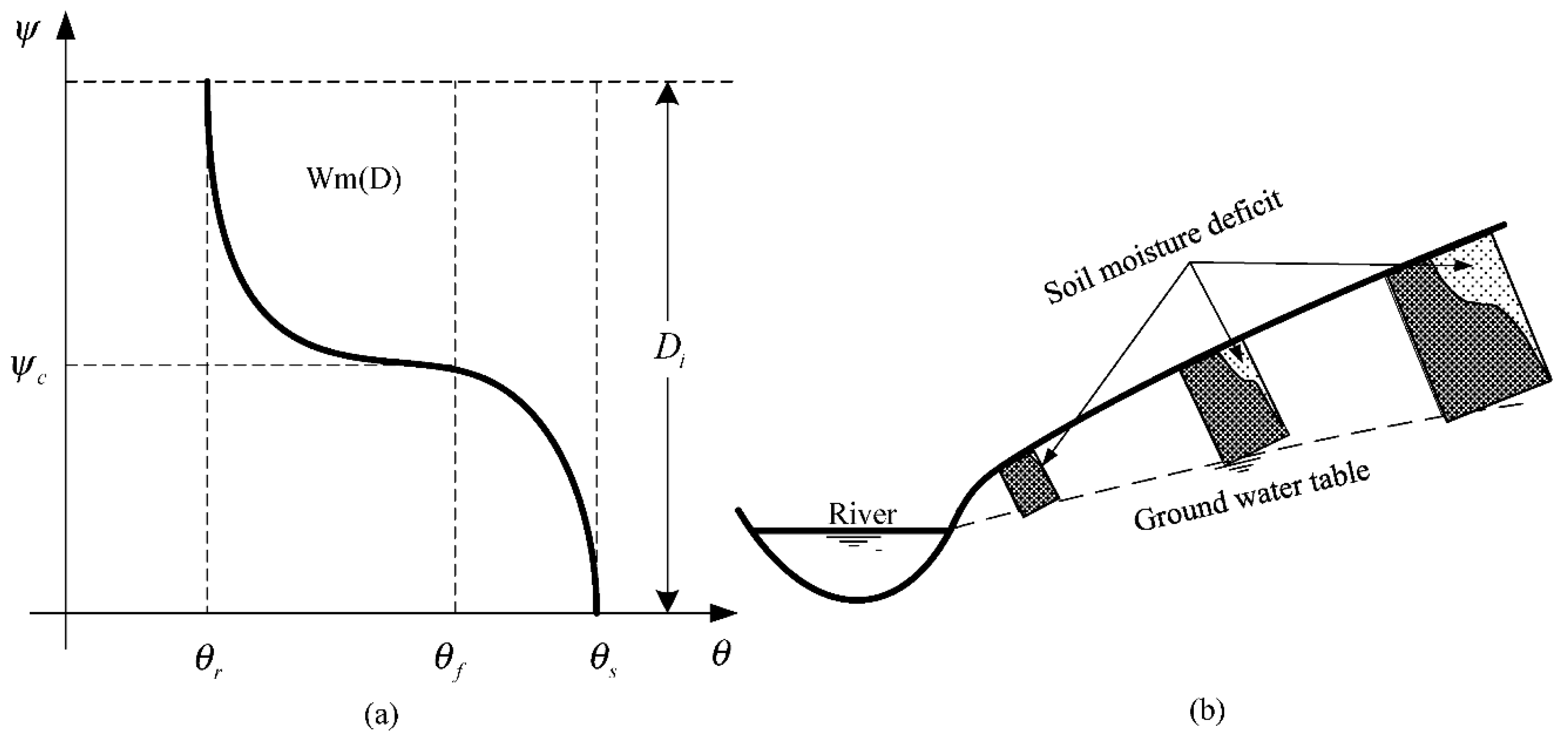
Figure 2.
Location and topography in Ziluoshan basin.
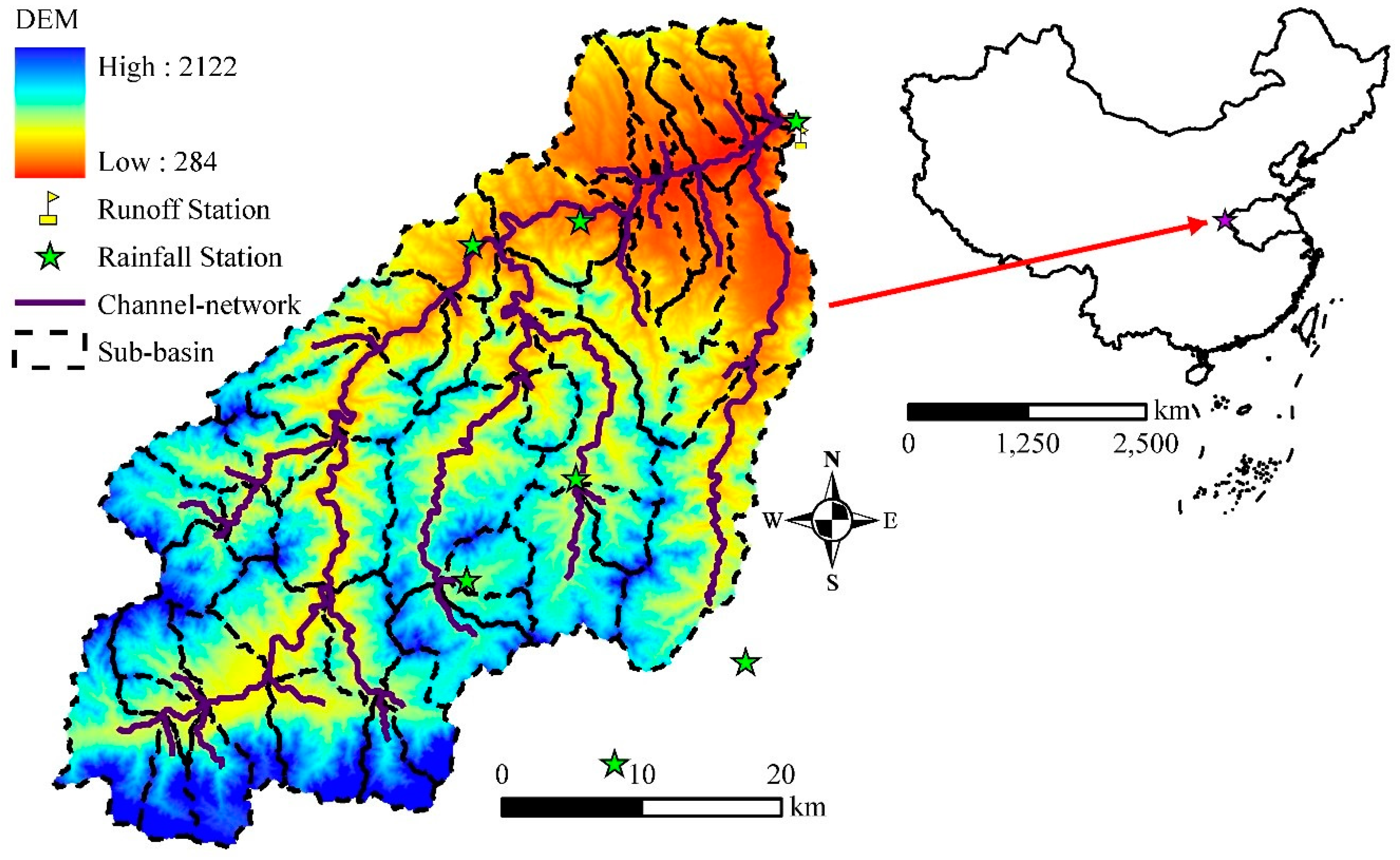
Figure 3.
Percentage of sand and clay within the soil depth of 0–1.0 m, (a) Percentage of sand and (b) Percentage of clay.
Figure 3.
Percentage of sand and clay within the soil depth of 0–1.0 m, (a) Percentage of sand and (b) Percentage of clay.
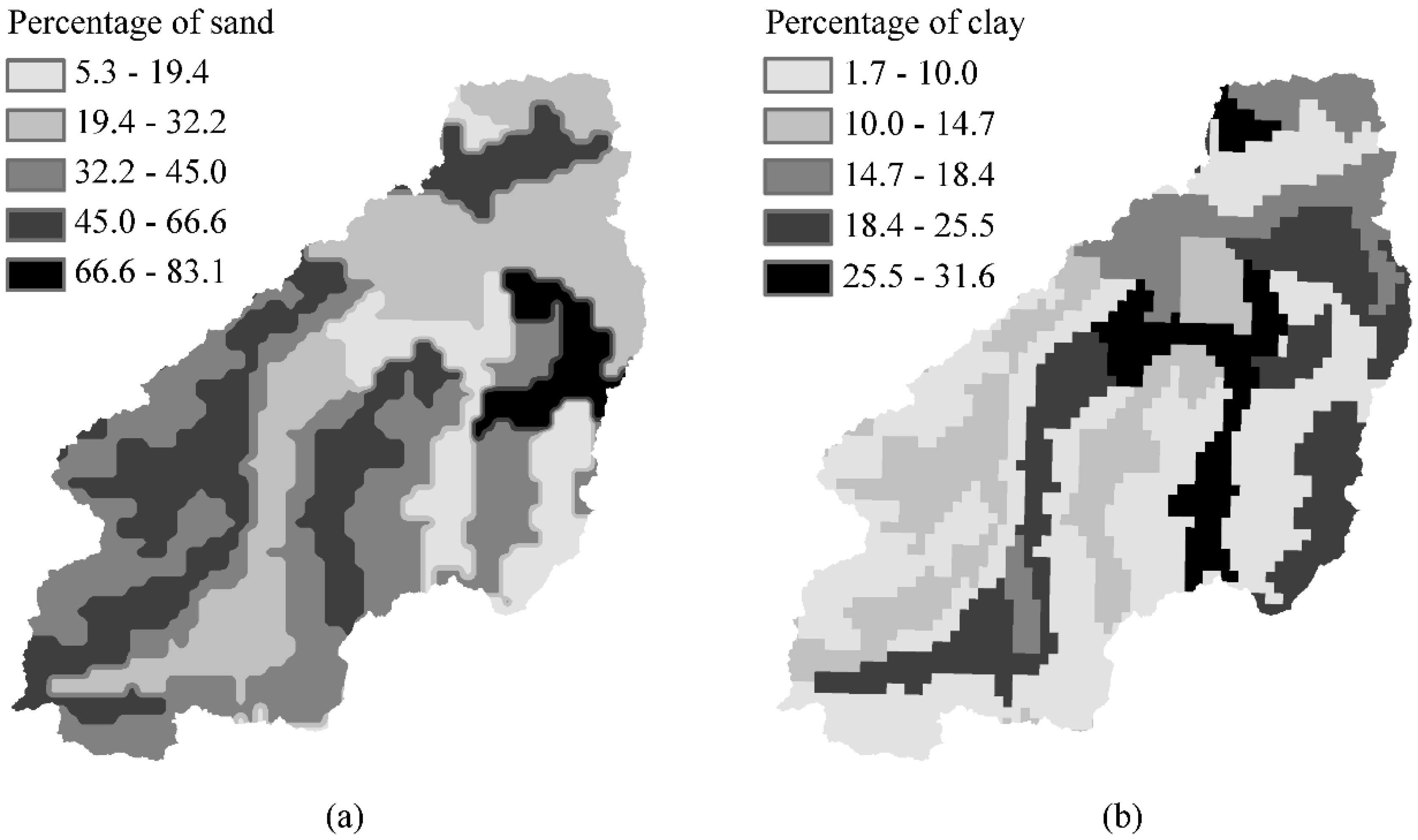
Figure 4.
Spatial distribution of storage capacity WM (basin mean value of local storage capacity). (a) Cumulative frequency (cumulative proportion of partial basin area versus total basin area) of Wm ~ f/F in terms of Equation (13) for the 50 sub-basins, (b) sub-basin mean WM.
Figure 4.
Spatial distribution of storage capacity WM (basin mean value of local storage capacity). (a) Cumulative frequency (cumulative proportion of partial basin area versus total basin area) of Wm ~ f/F in terms of Equation (13) for the 50 sub-basins, (b) sub-basin mean WM.
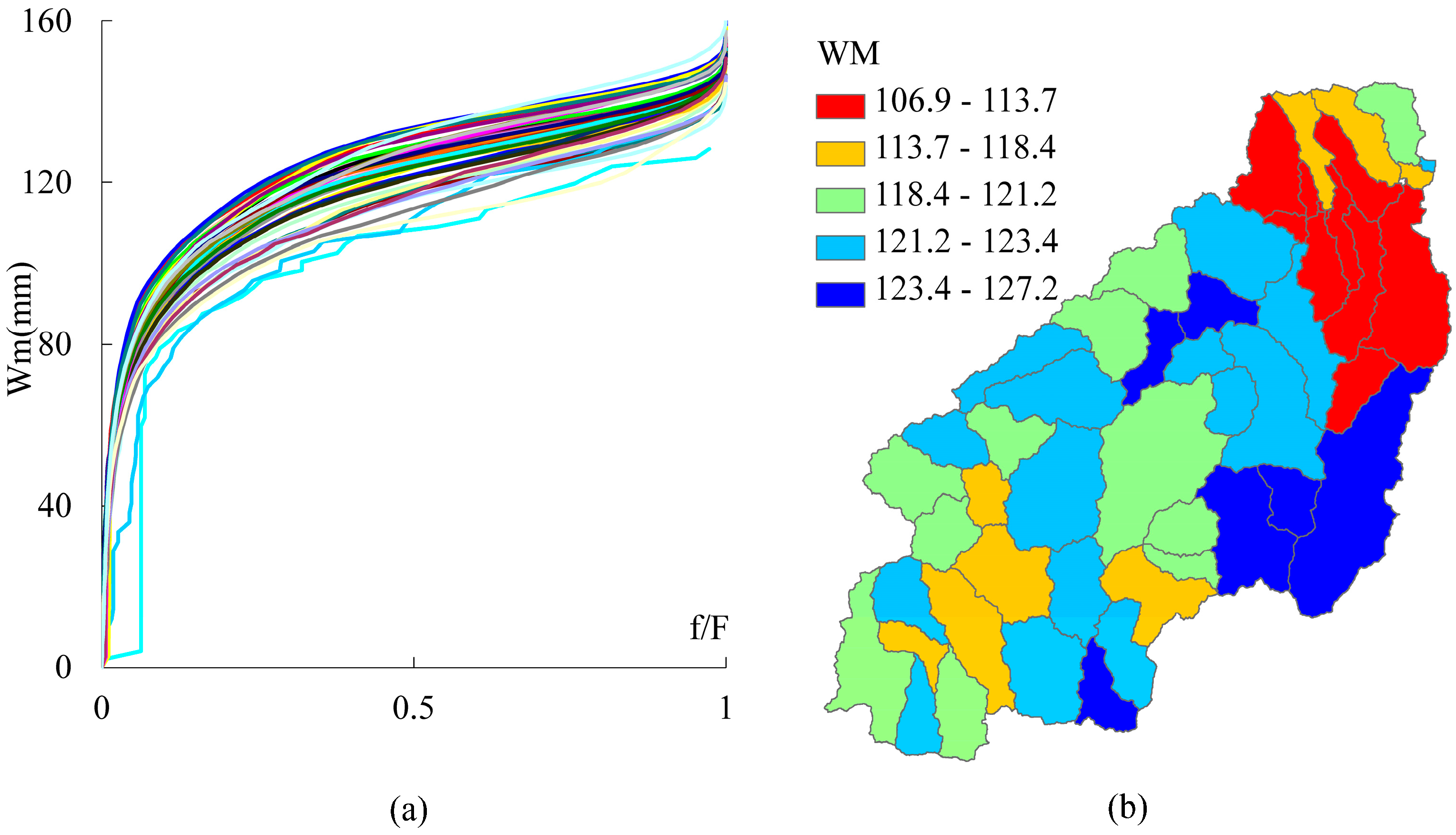
Figure 5.
Hourly simulated and observed runoff in the watershed for the selected flooding events.
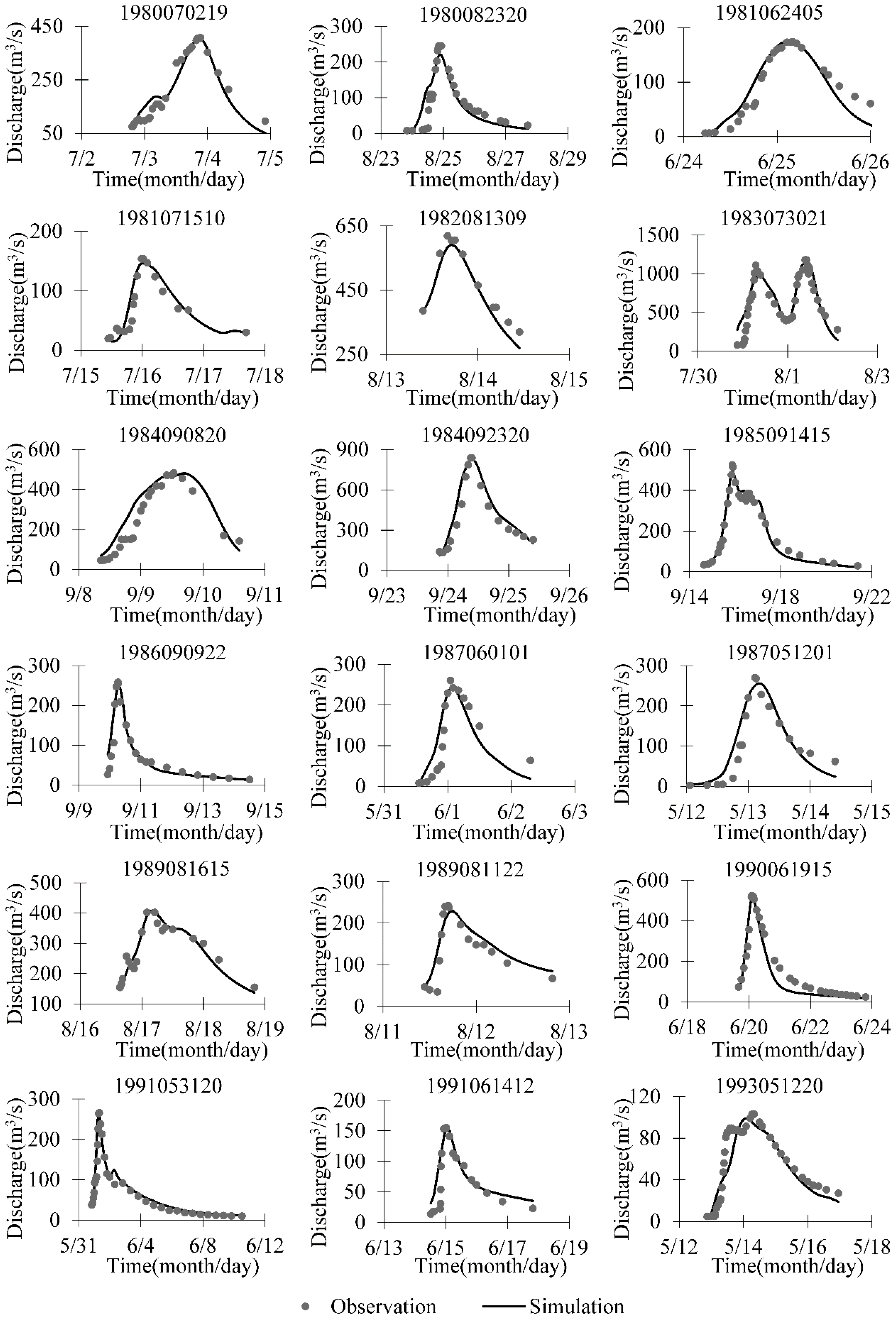
Figure 6.
Distribution of soil moisture storage capacity Wm related to Szm (‘effective depth’ that determines the decay of hydraulic conductivity with depth) in the whole watershed (a) and sensitivity of parameter Szm to runoff R and watershed mean storage capacity WM (basin mean value of local storage capacity) for the flood period during 11 May–23 September, 1985 (b).

Figure 7.
Relationship between sub-basin mean WM (basin mean value of local storage capacity) and topographic index for 50 sub-basins with soil types of silt, sandy loam and clay, respectively. (Note: catchment mean Szm (‘effective depth’ that determines the decay of hydraulic conductivity with depth) is assumed as 42.8 mm in the figure). (a) And simulated flood discharges for sand, sand loam and clay in 1985 (b).

Figure 8.
Spatial variation of mean annual precipitation (a) and runoff (b) during 1980–1996 and spatial variation of soil moisture content (c) and actual evaporation (d) on 1 October 1987.
Figure 8.
Spatial variation of mean annual precipitation (a) and runoff (b) during 1980–1996 and spatial variation of soil moisture content (c) and actual evaporation (d) on 1 October 1987.


Table 1.
Van Genuchten parameters for three types of soil [24].
Table 1.
Van Genuchten parameters for three types of soil [24].
| Parameter | Sand | Loam | Clay |
|---|---|---|---|
| θs | 0.37 | 0.46 | 0.51 |
| θr | 0.058 | 0.083 | 0.102 |
| α (cm−1) | 0.035 | 0.025 | 0.021 |
| n | 3.19 | 1.31 | 1.2 |
Table 2.
Calibrated parameter values of the modified Xin’anjiang model [43].
Table 2.
Calibrated parameter values of the modified Xin’anjiang model [43].
| Parameter | Explanation | Unit | Lower Bound | Upper Bound | Value |
|---|---|---|---|---|---|
| Runoff Generation Calculation | |||||
| KC | Ratio of potential evapotranspiration to pan evaporation | 0.6 | 1.2 | 0.7 | |
| WM | Areal mean tension water capacity | mm | 92–127 | ||
| Szm | Scaling parameter based on soil properties | mm | 10 | 1000 | 42.8 |
| C | Deeper evapotranspiration coefficient | 0.08 | 0.18 | 0.17 | |
| Water Source Separation | |||||
| SM | Free water storage capacity | mm | 5 | 50 | 5/15 |
| EX | Exponential of the distribution of water capacity | 1 | 1.5 | 1.5 | |
| KG | Outflow coefficient of free water storage to the groundwater flow | 0.2 | 0.6 | 0.4 | |
| KI | Outflow coefficient of free water storage to the interflow | 0.2 | 0.6 | 0.3 | |
| Concentration Calculation | |||||
| CS | Recession constant of surface water storage | 0 | 0.7 | 0.1/0.2 | |
| CI | Recession constant of interflow storage | 0.5 | 0.9 | 0.5/0.7 | |
| CG | Recession constant of groundwater storage | 0.5 | 0.998 | 0.995/0.98 | |
| KE | Residence time of water | h | 0.5 | 1.5 | 1 |
| XE | Muskingum coefficient | 0 | 0.5 | 0.3 | |
Note: for */*, the upper and lower values represent calibrated parameter values for daily and hourly simulations in the following verification, respectively.
Table 3.
Results of model calibration and validation using daily data.
| Period | Year | Annual P | Annual E | R (mm) | RE (%) | RMSE | NSC | |
|---|---|---|---|---|---|---|---|---|
| (mm) | (mm) | Obs | Sim. | (mm) | ||||
| Calibration | 1979 | 898.3 | 542.3 | 227 | 226.1 | −0.42 | 1.1 | 0.77 |
| 1980 | 792 | 470.6 | 188.1 | 196.1 | 4.24 | 1.0 | 0.73 | |
| 1981 | 653.6 | 464.4 | 94.6 | 98.4 | 3.99 | 0.6 | 0.58 | |
| 1982 | 1096.3 | 435.3 | 551.1 | 523.1 | −5.06 | 4.4 | 0.91 | |
| 1983 | 1222.8 | 519.1 | 644.3 | 607.1 | −5.78 | 2.8 | 0.87 | |
| 1984 | 984.6 | 557 | 362.1 | 337.9 | −6.69 | 1.5 | 0.78 | |
| 1985 | 873.5 | 489.5 | 296.4 | 298.4 | 0.68 | 1.5 | 0.78 | |
| 1986 | 596.1 | 433.4 | 80.9 | 79.5 | −1.73 | 0.6 | 0.47 | |
| 1987 | 736.6 | 469.4 | 146.4 | 153.2 | 4.64 | 1.1 | 0.56 | |
| 1988 | 803.3 | 380.3 | 224.4 | 233.2 | 3.92 | 1.6 | 0.85 | |
| Mean | 865.7 | 476.1 | 281.5 | 275.3 | −0.22 | 1.6 | 0.73 | |
| Validation | 1989 | 854.6 | 408.6 | 257.9 | 268.8 | 4.23 | 1.4 | 0.74 |
| 1990 | 870.3 | 554.5 | 258.8 | 257.7 | −0.44 | 1.4 | 0.87 | |
| 1991 | 605.5 | 475.7 | 120.1 | 109.2 | −9.1 | 0.7 | 0.67 | |
| 1992 | 741.7 | 467.5 | 108.1 | 104 | −3.85 | 0.7 | 0.75 | |
| 1993 | 647.8 | 492.2 | 95.1 | 99.8 | 4.93 | 0.6 | 0.83 | |
| 1994 | 867.3 | 473.4 | 155.3 | 166 | 6.94 | 1.4 | 0.73 | |
| 1995 | 731.4 | 407.8 | 151.3 | 153.2 | 1.27 | 1.1 | 0.81 | |
| Mean | 759.8 | 468.5 | 163.8 | 165.5 | 0.57 | 1.0 | 0.77 | |
Table 4.
Results of model calibration and validation using hourly data.
| Flood No. | P | E | Flood Volume (106 m3) | Peak Discharge (m3/s) | RMSE | NSC | |||||
|---|---|---|---|---|---|---|---|---|---|---|---|
| (mm) | (mm) | Vobs | Vsim | RE (%) | Qobs | Qsim | RE (%) | (m3/s) | |||
| Calibration | 1980070219 | 32.4 | 5.7 | 41.6 | 39.4 | −5.28 | 408.0 | 407.3 | −0.18 | 30.9 | 0.94 |
| 1980082320 | 26.3 | 4.4 | 23.4 | 24.9 | 6.31 | 245.0 | 227.2 | −7.26 | 37.5 | 0.71 | |
| 1981062405 | 30.0 | 4.7 | 15.4 | 14.2 | −7.85 | 174.0 | 175.2 | 0.66 | 7.9 | 0.87 | |
| 1981071510 | 12.7 | 4.3 | 13.2 | 13.3 | 0.88 | 154.0 | 146.4 | −4.94 | 25.3 | 0.79 | |
| 1982081309 | 31.7 | 0.9 | 57.3 | 52.8 | −7.82 | 619.0 | 591.6 | −4.43 | 42.1 | 0.89 | |
| 1983073021 | 68.7 | 4.7 | 119.3 | 126.3 | 5.89 | 1180.0 | 1153.3 | −2.26 | 121.6 | 0.83 | |
| 1984090820 | 49.1 | 4.9 | 52.6 | 62.2 | 18.34 | 483.0 | 481.2 | −0.37 | 68.8 | 0.80 | |
| 1984092320 | 41.9 | 0.9 | 53.8 | 60.8 | 13.07 | 838.0 | 827.5 | −1.26 | 71.1 | 0.92 | |
| 1985091415 | 82.5 | 5.2 | 91.3 | 86.8 | −4.97 | 524.0 | 496.5 | −5.26 | 22.9 | 0.98 | |
| 1986090922 | 7.0 | 0.9 | 12.9 | 14.5 | 12.73 | 258.0 | 249.5 | −3.31 | 36.8 | 0.81 | |
| 1987060101 | 27.5 | 4.1 | 16.3 | 14.9 | −8.61 | 260.0 | 233.0 | −10.40 | 33.3 | 0.87 | |
| 1987051201 | 47.2 | 3.3 | 18.0 | 19.8 | 10.06 | 270.0 | 255.6 | −5.35 | 36.1 | 0.84 | |
| Mean | 38.1 | 3.7 | 42.9 | 44.2 | 2.73 | 451.1 | 437.0 | −3.70 | 44.5 | 0.85 | |
| Validation | 1989081615 | 111.0 | 13.7 | 116.9 | 110.3 | −5.71 | 402.0 | 408.1 | 1.51 | 29.7 | 0.93 |
| 1989081122 | 11.1 | 1.3 | 13.8 | 15.5 | 12.29 | 242.0 | 229.1 | −5.34 | 31.9 | 0.80 | |
| 1990061915 | 33.2 | 10.7 | 50.9 | 40.2 | −21.16 | 524.0 | 517.6 | −1.23 | 41.6 | 0.95 | |
| 1991053120 | 45.8 | 28.8 | 41.5 | 46.8 | 12.79 | 266.0 | 269.7 | 1.37 | 24.6 | 0.89 | |
| 1991061412 | 18.5 | 11.4 | 16.9 | 19.5 | 15.50 | 155.0 | 155.9 | 0.56 | 23.4 | 0.72 | |
| 1993051220 | 19.8 | 5.9 | 18.7 | 17.6 | −6.08 | 103.0 | 99.0 | −3.90 | 15.6 | 0.78 | |
| 1995072422 | 52.7 | 3.5 | 36.1 | 38.2 | 5.98 | 775.0 | 706.2 | −8.88 | 85.0 | 0.74 | |
| Mean | 41.7 | 10.8 | 42.1 | 41.2 | 1.94 | 352.4 | 340.8 | −2.27 | 35.6 | 0.83 | |
© 2017 by the authors. Licensee MDPI, Basel, Switzerland. This article is an open access article distributed under the terms and conditions of the Creative Commons Attribution (CC BY) license (http://creativecommons.org/licenses/by/4.0/).
Share and Cite
MDPI and ACS Style
Xiang, X.; Wu, X.; Chen, X.; Song, Q.; Xue, X. Integrating Topography and Soil Properties for Spatial Soil Moisture Storage Modeling. Water 2017, 9, 647. https://doi.org/10.3390/w9090647
AMA Style
Xiang X, Wu X, Chen X, Song Q, Xue X. Integrating Topography and Soil Properties for Spatial Soil Moisture Storage Modeling. Water. 2017; 9(9):647. https://doi.org/10.3390/w9090647
Chicago/Turabian StyleXiang, Xiaohua, Xiaoling Wu, Xi Chen, Qifeng Song, and Xianwu Xue. 2017. "Integrating Topography and Soil Properties for Spatial Soil Moisture Storage Modeling" Water 9, no. 9: 647. https://doi.org/10.3390/w9090647
Note that from the first issue of 2016, this journal uses article numbers instead of page numbers. See further details here.