Long-Term Assessment of Climate Change Impacts on Tennessee Valley Authority Reservoir Operations: Norris Dam


1
Sierra Nevada Research Institute, School of Engineering, University of California at Merced, Merced, CA 95344, USA
2
Civil and Environmental Engineering, Cleveland State University, Cleveland, OH 44115, USA
*
Author to whom correspondence should be addressed.
Water 2017, 9(9), 649; https://doi.org/10.3390/w9090649
Submission received: 6 February 2017
/
Revised: 25 July 2017
/
Accepted: 25 August 2017
/
Published: 30 August 2017
Abstract
:Norris Reservoir is the oldest and largest reservoir maintained and operated by the Tennessee Valley Authority (TVA). Norris Dam received a new operating guide in 2004; however, this new guide did not consider projected climate change. In an aging infrastructure, the necessity to assess the potential impacts of climate change on water resources planning and management is increasing. This study used a combined monthly hydrologic model and a general circulation model’s (GCM) outcome to project inflows for three future time spans: 2030s, 2050s, and 2070s. The current operating guide was then assessed and optimized using penalty-function-driven genetic algorithms to gain insight for how the current guide will respond to climate change, and if it can be further optimized. The results showed that the current operating guide could sufficiently handle the increased projected runoff without major risk of dam failure or inundation, but the optimized operating guides decreased operational penalties ranging from 22 to 37 percent. These findings show that the framework used here provides water resources planning and management a methodology for assessing and optimizing current systems, and emphasizes the need to consider projected climate change as an assessment tool for reservoir operations.
1. Introduction
Mid-19th century U.S. dams were constructed with a limited historical record of measured data, and by 2020 over 81 percent of these dams will have reached the average life-span of 50 years [1]. As hydro-climatic databases have expanded and the confidence in climate-model projections increased, climatological research results have continued to conclude that climate change will have various impacts on water-resource infrastructure [2,3]. The Intergovernmental Panel on Climate Change’s (IPCC) Fifth Assessment Report states that the period from 1983 to 2012 has likely been the warmest 30-year period in the past 1400 years, and that the globally averaged land and ocean temperature has linearly increased 0.85 °C since 1880 [3]. Studies focused on the implications of climate change show an increase in the probability of occurrence of extreme climatic events [3,4,5,6,7]. The southeastern United States has experienced increases in moderate to extreme summer droughts by 14 percent since the 1970s, and a 30 percent increase in annual average autumn precipitation since 1901 [8]. These increases have led to major infrastructure concerns regarding water supply and reservoir proficiency (inundation prevention, dam failure prevention, hydroelectric power generation, transportation, etc.) [9,10,11,12].
Developing new reservoir management strategies and modeling tools necessary for maintaining water-resource objectives and hydro-power generation, while considering the potential implications of projected climate change have become research topics of high demand [13,14,15,16]. Hamlet and Lettenmaier [17] used two global climate models and the Variable Infiltration Capacity (VIC) model to show that a temperature increase of 4.5 °C by 2095 led to earlier runoff, reducing flood control effectiveness and a 75 to 90 percent reduction in runoff volumes from April-September, leading to increased competition between energy production, irrigation, instream flow, and recreation for the Columbia River Basin. Stone et al. [18] used a Regional Climate Model and the Soil Water Assessment Tool to evaluate the temporal and spatial impacts of climate change on the water yield of the Missouri River Basin under a doubled CO2 scenario. They suggested revised reservoir release rules to supplement irrigation in the southern half of the Missouri River basin, where a reduced water yield was expected under their scenario. Christensen et al. [10] used a Parallel Climate Model with a business as usual greenhouse gas emissions scenario to drive the VIC model to assess the Colorado River Basin for three future periods (2010–2039, 2040–2069, and 2070–2098). By coupling runoff time series and reservoir-operation rules, they simulated that the mandated releases from Glen Canyon Dam to the Lower basins were met 59 to 75 percent of the time in the projected scenarios, respectively, compared to 92 percent in the historical climate simulation. Lee, Hamlet, Fitzgerald, & Burges [19] used the U.S. Army Corps of Engineers Hydrologic Engineering Center’s Prescriptive Model to optimize the flood rule curves for a suite of multi-objective reservoirs in the Columbia River Basin considering a warmer climate. They used linear penalty functions based on flood control and reservoir refill. Their findings showed that a warmer climate would reduce the effectiveness of the current reservoir operations, and that their optimized operations significantly reduced system storage deficits while maintaining current flood control reliability. These works have portrayed the need to assess reservoir operations considering projected climate change, and although much attention has been given to many large river basins in the United States, assessment of the Tennessee River Basin is limited [9].
In 2004, the Tennessee Valley Authority (TVA) performed a Reservoir Operation Study for 35 of the 49 reservoirs in their system to determine if modifications to their current operation policies could increase reservoir efficiency and, “produce greater overall public value” [20,21]. From this study, TVA designed a new multi-objective operating guide considering reservoir stability, hydropower generation, cooling requirements for downstream nuclear and fossil facilities, flood control, and navigation [20]. The new operating guide was to meet these objectives through maintaining reservoir water-surface elevations between two curves noted as the “flood guide” and “balancing guide”. The flood guide represents the maximum amount of storage attainable without risk of inundation or dam structural integrity, and the balancing guide ensures that all tributary reservoirs are drawn from equally when meeting downstream requirements. More importantly, this operating guide integrates the TVA reservoir system into a single network, providing the ability to systematically and efficiently monitor all reservoirs to maximize benefits and minimize risk governed by a hierarchy of operational demands. However, adaptability of this operating guide to climate change has yet to be examined.
This study used a combined multi-model approach with historical and projected climate scenarios to simulate inflow into one of the major Tennessee River Basin reservoirs to assess and optimize the current operating policy using a penalty-function driven genetic algorithm. The two main questions considered were: (1) Can Norris Reservoir sufficiently meet its requirements under its current operating guide considering a projected climate scenario? (2) How much can the operating policy of Norris Dam be improved if a projected climate scenario is considered?
2. Materials and Methods
This research developed a framework for assessing and optimizing a multi-purpose reservoir’s operating guide considering a projected climate scenario. This was accomplished using: (1) a combined multi-model approach, calibrated with historical inflow data and (2) 100 sets of inflow hydrograph realizations from a general circulation model (GCM) product as inputs to the combined hydrologic model. Then, the inflow hydrograph realizations were used to assess the current operating guide, considering historical and projected time spans. Finally, the operating guide was stochastically optimized to minimize the overall expected operational penalty using a genetic algorithm. To isolate the impacts of climate change on Norris Reservoir’s current policy, this study assesses these impacts as current conditions, negating the need to account for the effects of changes in land use, water demand, or socio-economics on this system.
2.1. Study Area
Completed in 1936, Norris Dam is the largest and oldest multi-purpose dam maintained and operated by TVA in the Tennessee River Basin [20]. Norris Dam serves as the pour point for the Upper Clinch and Powell Rivers which respectively drain 7542 and 2429 km2 southwesterly from the Appalachian Mountains of southwest Virginia into northeastern Tennessee. The elevation of the study area ranges from 268 to 1412 m above mean sea level (Figure 1) Norris Dam is located in northeastern Tennessee (36°13′27″ N, 84°05′29″ W), providing 1373 million cubic meters (MCM) of flood storage, cooling water for downstream power plants, generating a net of 110 megawatts of hydropower, and providing flows for recreation and ecosystem sustainability. Its inflowing subwatersheds are amongst the highest for supporting endangered aquatic species in North America [21], and offers many recreational benefits [22]. Norris Dam was selected for this study provided no other reservoirs supply inflow, allowing this study to isolate the effects of changes in climate, and remove the need to consider the TVA reservoir system.
The climate for this region is described as humid subtropical, consisting of hot, humid summers and mild winters [9,23]. Based on data obtained from the National Climatic Data Center (NCDC), the study region has an average annual precipitation of about 1087 mm, where most precipitation falls as rain, occasionally snow, with a slight increase in precipitation during late spring and early summer, and a decrease during the fall and early winter. The average annual temperature is 13.1 °C with monthly mean temperatures ranging from 5.7 to 26.0 °C.
2.2. Data Sources
2.2.1. Climatic Data
Data from seven NCDC stations were collected providing a minimum of 31 years of continuous precipitation (P) and temperature (T) records ranging from 1 January 1976 to 31 December 2006 (Figure 1). Temperature data was not available at stations VA448547 and VA449215. The temperature data was used to estimate potential evapotranspiration (PET), via the Thornthwaite method, for input into a hydrologic model [24]. This method was selected given it only requires temperature and latitude, and has been used in similar studies [24,25,26,27,28]. The calculated PET data was used in conjunction with the precipitation data to simulate inflow into Norris Reservoir.
2.2.2. Climate Projection Data
The National Center for Atmospheric Research, Community Earth System Model (CESM) 1.0 was the GCM used to project climate through the year 2100 due to its use in similar studies [6,29]. This GCM has a latitudinal and longitudinal resolution of 0.94 and 1.25 degrees, respectively, leading to six pixels needed to cover the study area. The Representative Concentration Pathway (RCP) 4.5 projection scenario was selected as it considers emission mitigation policies will be enacted during the 21st century [6,30,31,32,33]. CESM 1.0 precipitation and temperature data were subdivided into three time spans, 2030s, 2050s, and 2070s by taking the mean of the 15 years prior and post to the year of the time span name.
2.2.3. Dam Operations
The hierarchy of objectives of Norris Dam were obtained through direct discussion with TVA River Operations personnel. These data included daily full natural flow measurements into Norris Reservoir, outflow measurements from the dam, and the water elevations required for Norris Reservoir to meet specific objectives. Outflow requirements included the minimum outflow to maintain the downstream ecosystem, provide hydroelectric power generation, meet Bull Run fossil plant cooling requirements, and the maximum outflow with the outflow gate fully opened before overtopping. Water-surface elevation values included the historical maximum elevation, elevation compromising dam structural integrity, and the minimum elevations needed for reservoir maintenance and navigation. TVA stated the primary objective is to maintain Norris Reservoir’s water elevation between the flood and balancing guides (Figure 2).
Reservoir water elevation often exceeds the flood guide from January to March (Figure 2) [34]. TVA does not provide an explicit explanation but states that the primary operating objective is to maintain water elevation at or below the flood guide, and that the elevation may rise above the flood guide because of large inflows, but is subsequently lowered to the flood guide as soon as possible. They also state that they attempt to maintain water elevation at the flood guide from 1 June through Labor Day, the first Monday in September, to maximize recreation [34]. It is inferred that they aim to maintain elevation near the flood guide from January to mid-April to support summer recreation, and high-flow winter and spring storms result in water elevation exceeding the flood guide. The 2016 curve supports this inference as it appears that efforts to lower the elevation after high inflow events occurred (Figure 2).
2.3. Spatial Interpolation
Inverse distance weighting from the centroid of all GCM pixels was used to calculate composite-projection values to the coordinates of the meteorological stations [35,36]. These composite values were then spatially averaged to the study area using the Thiessen polygon values developed from the meteorological stations.
2.4. Climatic Data Reproduction
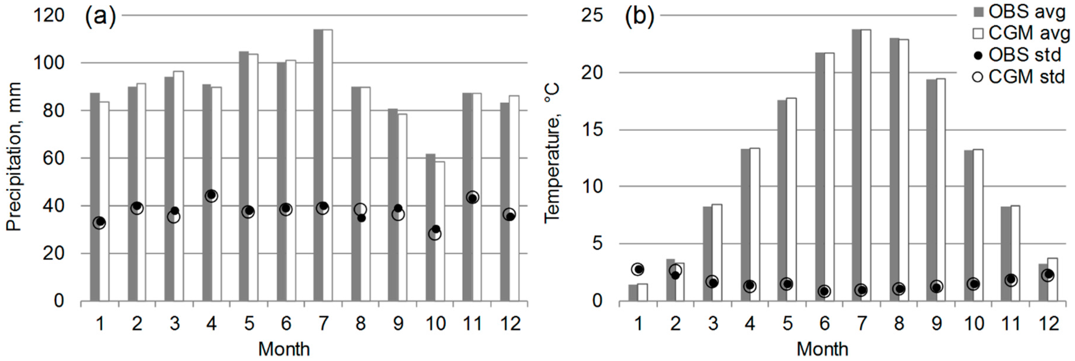
The Conditional Generation Method (CGM) tested by Kim and Kaluarachchi [37] was used to assimilate 100 instances of monthly temperature and precipitation for each time span. The 100 instances representing the historical observations are referred to as Base, whereas the projection scenarios maintain their respective names, 2030s, 2050s, and 2070s. The future projections were computed by applying the monthly changes (°C change for temperature and % change for precipitation) to the 100 sets of the Base scenario. CGM can capture both the temporal and inter-station correlation of meteorological data. It also considers the randomness of occurrences characterized by the historical climate data. This makes it preferable for hysteretic time series, because it preserves seasonality by considering the conditional probability associated with the transition from successive months, where uncorrelated random Monte Carlo simulations selects values evenly from the entire dataset and therefore does not capture seasonality. The monthly mean and standard deviation of climate time series generated by CGM (i.e., Base) are compared with the observed dataset to verify the performance of CGM outputs (Figure 3).
2.5. Hydrologic Model
A combined multi-model approach was used to generate the hydrologic model in this study. Methods used were multiple linear regression (MLR) [11,37,38,39,40,41,42,43], a conceptual-water-balance model (TANK) [9,37,44,45,46,47], and an artificial neural network (ANN) [48,49,50,51,52]. The strength of each method was assessed based on its ability to more accurately simulate specific characteristics of observed runoff.
Inputs into the MLR and ANN were determined using stepwise regression with a p-value threshold <0.05 for the variables PETt, PETt−1, Pt, and Pt−1, where t is the current time-step’s month and t − 1 is the previous time-step’s month. The TANK model only required PETt, and Pt due to accounting for real-time soil moisture, thus inherently hysteretic. Although snowmelt was not explicitly modeled, the relationship between precipitation and temperature were included in the MLR and ANN models, while the TANK model only considered above freezing conditions. To overcome the drawbacks of any individual model, the three models were individually calibrated (or trained) and validated using historical climate-runoff dynamics (i.e., inflow hydrographs), and were then combined using a numerical optimization technique to find global optimal weighting factors that minimize the sum of square error between the modeled and observed data. Therefore, the objective function (OBJHM) can be expressed as:
where ln is the natural logarithm, OBSt is the observed runoff at month t, SIMt is the weighted runoff using the three simulated runoff values at month t, w is the weighting factor derived for each individual rainfall-runoff model, and N is the total number of time steps.
SIMt = w1 × MLRt + w2 × TANKt + w3 × ANNt for w1 + w2 + w3 = 1
2.6. Reservoir Routing Optimization
The operating guide for Norris Dam was optimized by minimizing the cumulative penalty generated from a penalty function through altering the flood and balancing guidelines. Routing of Norris Reservoir was simulated using the estimated runoff generated from the combined hydrologic model, reservoir objectives and release requirements, and the current and optimized operating guides. Reservoir elevation was determined using the Norris Reservoir elevation-storage chart provided by TVA [53], and performing a mass balance of the reservoir at each time-step t, computed as:
where is the available storage of the reservoir with a minimum of Smin and maximum of Smax, is the monthly inflow, Oi is the monthly required outflow for objective i from 1 to m (i.e., hydropower generation, fossil power plant cooling water, instream flow, etc.), and is the monthly withdrawal directly from the reservoir. was viewed as zero because no significant water withdrawals were reported for Norris Reservoir. Outflow was set to be the minimum allowed flow (Omin) to meet all requirements given the reservoir elevation, or the maximum (Omax or Smax) if dam structural integrity was threatened. Maximum or minimum requirements of outflow or water elevation during reservoir operation are provided in Table 1. The final outputs for any time-step are reservoir elevation, O, and S. This study considered the deterioration of storage volume (S) by sediment deposition using a nonlinear regression based on elevation-storage curves from 1936 to 1970 predicted by the TVA [53]. The exponential regression function showed an annual storage decrease about 0.02 percent with R2 = 0.98.
subject to Omin ≤ Ot ≤ Omax and Smin ≤ St ≤ Smax
At the end of each time step t, penalty values were added to the objective function (Equation (3)) if the routing results (outflow and/or elevation) violated any individual operating rule (Table 1). The penalty function generated for this study consisted of five inflow and three outflow penalties. Provided reservoir operational monetary and non-monetary benefits or penalties lack a standard or concrete method of quantification, this study assigned a weighted-sum aggregation of conceptually-driven mathematical penalty functions and values based on operational priorities set by TVA [54,55,56] (Table 1). Penalty functions and values were constant for the future simulation time periods as the primary objective of this study is to assess the current operation policy with respect to potential climate change. Although this approach has been used in similar studies, it may increase uncertainty in the results due to potential misrepresentation of any given penalty [19]. It should be stated that the values do not represent any real penalty to incur, but aim to represent the degree of violation for failing to meet a specific objective.
This study assigned a quadratic-function flood-risk penalty for reservoir elevations between the flood guide and the historical maximum, and between the balancing guide and minimum elevation required for navigation (Table 1). The penalty for exceeding the flood guide (FG), received the value of (EL-FG)2 up to the historical maximum water elevation (1030.38 ft), which has a maximum penalty of 923, (1030.38 − 1000)2, during January, February, March, November, and December. Similarly, the penalty for reservoir elevation between the balancing guide (BG) and minimum elevation for navigation (NAV) received a penalty value equal to (BG-EL)2. By using a quadratic function, if reservoir elevation deviates from the flood or balancing guide the penalty value exponentially increases, resulting in a more aggressive penalty minimization by the optimization algorithm. However, when applying the same quadratic penalty function from the historical maximum elevation to the top of gate (1034 ft), the penalty only increases to 1156, (1034 − 1000)2, for winter and 196, (1034 − 1020)2, for summer, resulting in frequent violations due to producing mild penalties relative to their importance. Therefore, this study used a step function for reservoir objectives of greater importance (one order of magnitude for each step) based on the maximum flood guide penalty of 1000 (approximate of 923), so that the penalty for reservoir elevations between the historical maximum and top of gate is set to 103, and is 104 when exceeding the top of gate. The last flood related penalty, flooding downstream (FLD), which counts the risk of inundation in downstream areas due to excessive discharge, received a penalty of 104. The COOL penalty was evaluated similarly to NAV considering its relative importance to dam safety and functionality because the Bull Run Fossil Plant is located about 45 km downstream from Norris Dam. Increasing penalties by an order of magnitude increases the optimization algorithm’s ability to better represent the relative importance of specific objectives.
The numerical setting of these penalties was developed to avoid dam structural and operational failure. Each set of inflow hydrographs yielded the cumulative individual penalty over the simulation time span and the sum of penalties for each scenario (100 inflow realization sets of 360 months per scenario). Therefore, the penalty objective function (OBJP) can be formulated as follows:
where E is the expectation operator used to compute the mean penalty value over the 100 monthly CGM-generated hydrographs as input into the combined hydrologic model, Penalty is the penalty value computed for each monthly requirement based on Table 1, and constraint conditions are set by Equation (2) and Table 1. The goal is to find optimal flood and balancing guides for each month, while minimizing the cumulative penalty averaged across the 100 realizations.
The optimized operating guides were generated using genetic algorithms to minimize the mean of the 100 CGM realizations’ penalty values. Genetic algorithms have become an increasingly popular method for optimizing reservoir operations in recent decades [57,58,59]. The settings for the genetic algorithm used in this study were: (1) 100 for the number of generations; (2) 0.1 for termination tolerance on objective function value; (3) 0.001 for termination tolerance on constraints; (4) 30 for the population size; (5) 20 for the stall generations; (6) the adaptive feasible function for a mutation function; and (7) the heuristic function for a crossover function. Initial population is assumed as the current flood and balancing guide with the initial water level set to (January) of the 30-year average from 1976 to 2005.
2.7. Reservoir Assessment
Norris Reservoir’s operating guide was assessed using three scenarios. First, that TVA maintained their current operating guide throughout all three time spans, denoted as Current. Second, that TVA optimized their operating guide as a function of the historical inflow into the reservoir, denoted as Base-Opt. Third, TVA optimized their operating guide for each time span as a function of the GCM projected inflow into the reservoir, denoted individually as 2030-Opt, 2050-Opt and 2070-Opt, or collectively as GCM-Opt. Scenario performance was determined by comparing the percent change of cumulative penalty of Base-Opt and GCM-Opt with the Current scenario for each time span.
3. Results
3.1. Generation of Composite Climate Data
Projected temperature data showed mean annual changes of −0.42, 0.34, and 0.89 °C compared to the historical mean for the 2030s, 2050s and 2070s, respectively. The 2030s showed increases in mean monthly temperatures from January–April, and decreases from May–December. The 2050s showed increases in temperature from January–May and September–December, with decreases from June–August. The 2070s showed increases in temperature for all months except July. The most significant variance was observed as increases during winter months (January–March) and a decrease in July (historically the hottest month) for all three time spans.
Projected precipitation resulted in an increase for most months. Observed increases in mean annual precipitation relative to the historical mean were approximately 14, 18 and 20 percent for the 2030s, 2050s and 2070s, respectively. The largest increases were observed in July and August for all time spans. The 2030s showed increases in precipitation for all months except January, February, May and September, the 2050s showed increases for all months except February, May and September, and the 2070s showed increases for all months except September.
3.2. Hydrologic Model Evaluation
The individual models were evaluated using various performance statistics to consider the overall model strength (coefficient of determination), annual and seasonal predictions, and flow duration similarity (Table 2). The TANK model performed worst overall, but performed best at simulating peak flows. The MLR model performed best simulating annual runoff, the high flow season, and peak low runoff. The ANN model performed best overall with an R2 of 0.81, and best at simulating the low flow season and the inter-quartile range of the observed runoff distribution.
The combined hydrologic model had a coefficient of determination of 0.81, and adequately compared to the historical runoff data in accounting for seasonality and peak high runoff (Figure 4). The combined hydrologic model did not always outperform the individual models, but performed at least second best in all tests but two (underlined in Table 2). It was determined that under performance in these tests were not a concern, given low flow season error was still small, and 90th percentile high runoff was the result of extreme single events that was outside the scope of this study due to the coarse temporal resolution (monthly time step) of the GCM data.
3.3. Projected Changes in Runoff
The modeled runoff resulted in approximately 20.5, 24.0, and 24.5 percent increases from the Base runoff for the 2030s, 2050s, and 2070s respectively (Figure 5). When compared at a monthly time step, it was observed that runoff increased in all months, except February. The 2030s had the highest runoff compared to all projected scenarios in March and November, the 2050s in January, July, August and December, and the 2070s in April, May, June, September, and October.
3.4. Reservoir Routing and Optimization
Cumulative penalties were calculated individually and aggregated over the entire simulation (Table 3). Base-Opt showed decreases in cumulative penalty ranging from 22.2 to 24.4 percent compared to the Current scenario, yet it was greatly outperformed by the GCM-Opt scenarios showing cumulative penalty decreases of 35.4, 34.6 and 37.0 percent for the 2030s, 2050s and 2070s, respectively (Table 4). HM, NAV, TG, and ECOPOW penalties were not triggered by any simulation. Other than the Base time span, all other time spans and scenarios received FLD penalties. Penalties for COOL and FLD increased incrementally for all scenarios from the Base to 2050s, but 2070s penalties were in between the Base and 2030s for all scenarios.
The largest difference between the optimized balancing and historical guides occurred during the first five months of the year (Figure 6). The flood guides from January through April were increased for all scenarios, and most noticeable for 2050s-Opt and 2070s-Opt. All scenarios showed slight to large decreases in May. The balancing guides only showed noticeable change in April and May, with decreases from the historical values. This led to either a larger range between the flood and balancing guides for January through May, or a smaller range from June through September for most scenarios.
4. Discussion
All three projected scenarios showed the least change, or decrease, in temperature during summer months when compared to the historical data. The data suggests that increased precipitation during summer months (June–August) led to increased cloud cover. Further explaining why all three time spans showed decreases in temperature in July, as precipitation increased by a least 32 percent. This observation has also been cited by a study focusing on shifts in land cover as a result of climate change [60].
The percent increases in runoff exceeded the percent increases in precipitation for all projected scenarios. This is specifically counter intuitive for the 2050s and 2070s, where higher annual temperatures are projected, leading to increased annual evaporative demand. The monthly data showed that some of the more energy-limited months (March, April, and December) projected significant increases in precipitation with slight increases in temperature. This suggests an increase of rain versus snow events while evaporative demand is limited. During the summer months, July and August show significant increases in precipitation with slight decreases in temperature for all projected scenarios except for August in the 2070s, indicating lower evaporative demand with increased precipitation resulted in increased runoff. The 2030s showed increases of nearly 100 MCM for both February and September compared to the Base scenario. Further investigation showed that precipitation was marginally higher, and temperature significantly lower in these months compared to the other projected time spans, suggesting that the observed increase in runoff was due to the decrease in temperature, limiting evapotranspiration.
The results showed that the decrease in cumulative penalty with incrementing time span and scenario was almost all attributed to decreases in the FG and BG penalties. The data suggests that the increased inflow maintained reservoir storage near the flood guide, minimizing BG penalties. A major caveat for permitting reservoir storage to be maintained near the flood guide was the introduction of flooding downstream (FLD) penalties (Table 3). Although the 2070s had the highest percent increase in water-year precipitation, the FLD penalties for all scenarios under this time span were nearly or more than 50 percent less compared to the 2030s and 2050s. This can be explained in part by the 2070s having a lower inflow standard deviation and events exceeding the ninetieth and ninety-fifth percentile compared to the 2030s and 2050s, suggesting less extreme inflow events and more evenly distributed inflow throughout the water year in the 2070s.
The penalty for not meeting outflow requirements for Bull Run Fossil Plant cooling (COOL) slightly increased for all three projected time spans relative to Base. The data suggests that these increases in penalties were to rapidly return reservoir elevation above the balancing guide to prevent cumulative penalties from COOL and NAV, or the more extreme ECOPOW penalty, from being triggered.
All optimized flood guides were decreased during historically low flow months (Figure 6). With the climate projections showing substantial percent increases in runoff during dry months (from April to August) for all future time spans (Figure 5), having these guidelines lowered during dry months provides an extra buffer to prevent extreme reservoir elevations. On the other hand, all future time spans showed increases in the flood guide from January to March. These increases are caused in part by the carryover from the substantial increase in runoff in December for all future time spans (Figure 5). Increasing the flood guide during these months was the solution of the genetic algorithm to minimize the FG penalty. Further, increasing the flood guides during the earlier months of the year benefit managers, as it reduces the amount reservoir elevation needs to be raised to maintain objective satisfaction during the low-flow season.
5. Conclusions
Studies such as these provide beneficial information and tools promoting more efficient and effective water-resources planning and management. The results from this study concluded that runoff in this region is anticipated to increase over the next century as the result of an increase in precipitation with warmer winters leading to more rain versus snow events, and cooler summers reducing evaporative demand. Such a significant increase in runoff emphasizes the need for water resources management to reassess their systems considering projected climate change. This study provides insight for how the impacts of climate change may affect the performance of a multi-purpose reservoir if not considered, and that optimizing the current operating guide to consider a projected climate scenario reduced operational penalties by a minimum of 22.2 percent, and as much as 37.0 percent.
Increases in the flooding downstream penalty were observed in the projected scenarios. This could lead to dam structural integrity concerns, especially when considering individual storm hydrographs. Although Norris Dam could sufficiently handle the increased inflows, it is one of the Northern most dams and the increased flooding downstream may cause potential hazards for downstream dams. Therefore, the next phase of this research is to extend the scope to encompass reservoirs downstream of Norris, and eventually the entire TVA multi-dam network. It is also recommended that this analysis be performed again once the temporal resolution of GCM models are able to capture individual storm events.
This study provides a framework for assessing and optimizing reservoir routing. For the TVA, this framework showed that the current operating policy can be further optimized, and suggests that their current routing policies be reassessed considering climate change. Finally, this study shows the benefits of using genetic algorithms for assessing and optimizing reservoir routing guides, regardless of the objective or climatic regime.
Acknowledgments
This work was supported by the United States Geological Survey’s State Water Resources Research Institute Program under Grant 2013TN100B.
Author Contributions
Ungtae Kim and Joseph Rungee conceived and designed the experiments; Ungtae Kim guided the entire study and developed the Matlab codes for CGM, reservoir routing, penalty functions, TANK, and combined hydrologic model; Joseph Rungee developed the Matlab codes for MLR and ANN; Joseph Rungee contributed to collecting hydrologic data and GIS maps, performing numerical experiments, and communicating with TVA personnel; Ungtae Kim and Joseph Rungee analyzed and interpreted the results; Joseph Rungee prepared the initial draft and Ungtae Kim revised the manuscript.
Conflicts of Interest
The authors declare no conflict of interest.
References
- National Inventory of Dams. Available online: nid.usace.army.mil (accessed on 28 August 2017).
- Frederick, K.D.; Major, D.C. Climate Change and Water Resources. In Climate Change and Water Resources Planning Criteria; Frederick, K.D., Major, D.C., Stakhiv, E.Z., Eds.; Springer: Dordrecht, The Netherlands, 1997; pp. 7–23. [Google Scholar]
- Stocker, T.F.; Qin, D.; Plattner, G.K.; Tignor, M.; Allen, S.K.; Boschung, J.; Nauels, A.; Xia, Y.; Bex, V. IPCC, 2013: Climate Change 2013: The Physical Science Basis; Contribution of Working Group I to the Fifth Assessment Report of the Intergovernmental Panel on Climate Change; Midgley, P.M., Ed.; Cambridge University Press: Cambridge, UK; New York, NY, USA, 2013. [Google Scholar]
- Allen, M.R.; Ingram, W.J. Constraints on future changes in climate and the hydrologic cycle. Nature 2002, 419, 224–232. [Google Scholar] [CrossRef] [PubMed]
- Bell, J.L.; Sloan, L.C.; Snyder, M.A. Regional changes in extreme climatic events: A future climate scenario. J. Clim. 2004, 17, 81–87. [Google Scholar] [CrossRef]
- Gao, Y.; Fu, J.S.; Drake, J.B.; Liu, Y.; Lamarque, J.F. Projected changes of extreme weather events in the eastern United States based on a high resolution climate modeling system. Environ. Res. Lett. 2012, 7, 44025. [Google Scholar] [CrossRef]
- World Meteorological Organization (WMO). Statement on the Status of the Global Climate in 2013; WMO: Geneva, Switzerland, 2013. [Google Scholar]
- Karl, T.R. Global Climate Change Impacts in the United States; Cambridge University Press: Cambridge, UK, 2009. [Google Scholar]
- Choi, Y.G. Potential Impacts of Climate Change on Water Resources and Water Quality of Norris Lake, Tennessee. Master’s Thesis, University of Tennessee, Knoxville, TN, USA, 2011. [Google Scholar]
- Christensen, N.S.; Wood, A.W.; Voisin, N.; Lettenmaier, D.P.; Palmer, R.N. The effects of climate change on the hydrology and water resources of the Colorado River basin. Clim. Chang. 2004, 62, 337–363. [Google Scholar] [CrossRef]
- Helton, J.C.; Johnson, J.D.; Sallaberry, C.J.; Storlie, C.B. Survey of sampling-based methods for uncertainty and sensitivity analysis. Reliab. Eng. Syst. Saf. 2006, 91, 1175–1209. [Google Scholar] [CrossRef]
- Payne, J.; Wood, A.; Hamlet, A. Mitigating the effects of climate change on the water resources of the Columbia River Basin. Clim. Chang. 2004, 62, 233–256. [Google Scholar] [CrossRef]
- Arnell, N.W. Climate change and global water resources. Glob. Environ. Chang. 1999, 9, S31–S49. [Google Scholar] [CrossRef]
- Askew, A.J. Climate Change and Water Resources. In The Influence of Climate Change and Climatic Variability on the Hydrologic Regin and Water Resources, Proceedings of the Vancouver Symposium Soloman, Vancouver, BC, Canada, 9–22 August 1987; Solomon, S.I., Beran, M., Hogg, W., Eds.; IAHS Press: Wallingford, Oxfordshire, UK, 1987. [Google Scholar]
- Guegan, M.; Madani, K.; Uvo, C.B. Climate Change Effects on the High Elevation Hydropower System with Consideration of Warming Impacts on Electricity Demand and Pricing; A White Paper from the California Energy Commission’s California Climate Change Center; California Energy Commission: Sacramento, CA, USA, 2012. [Google Scholar]
- Markoff, M.S.; Cullen, A.C. Impact of climate change on Pacific Northwest hydropower. Clim. Chang. 2008, 87, 451–469. [Google Scholar] [CrossRef]
- Hamlet, A.F.; Lettenmaier, D.P. Effects of climate change on hydrology and water resources in the Columbia River Basin1. J. Am. Water Res. Assoc. 1999, 35, 1597–1623. [Google Scholar] [CrossRef]
- Stone, M.C.; Hotchkiss, R.H.; Hubbard, C.M.; Fontaine, T.A.; Mearns, L.O.; Arnold, J.G. Impacts of climate change on Missouri River Basin water yield. J. Am. Water Res. Assoc. 2001, 37, 1119–1129. [Google Scholar] [CrossRef]
- Lee, S.Y.; Hamlet, A.F.; Fitzgerald, C.J.; Burges, S.J. Optimized flood control in the Columbia River Basin for a global warming scenario. J. Water Res. Plan. Manag. 2009, 135, 440–450. [Google Scholar] [CrossRef]
- Tennessee Valley Authority. Reservoir Operations Study Final Programmatic Environmental Impact Statement; Tennessee Valley Authority: Knoxville, TN, USA, 2004.
- The United States Environmental Protection Agency (USEPA). Powell Valley Watershed Ecological Risk Assessment; USEPA: Washington, DC, WA, USA, 2002.
- Tennessee Valley Authority: Norris Reservoir. Available online: http://www.tva.gov/sites/norris.htm (accessed on 28 August 2017).
- Parker, J.M. The Influence of Hydrological Patterns on Brook Trout (Salvelinus Fontinalis) and Rainbow Trout (Oncorhynchus Mykiss) Population Dynamics in the Great Smoky Mountains. Master’s Thesis, University of Tennessee, Knoxville, TN, USA, 2008. [Google Scholar]
- Thornthwaite, C.W. An approach toward a rational classification of climate. Geogr. Rev. 1948, 38, 55–94. [Google Scholar] [CrossRef]
- Black, P.E. Revisiting the Thornthwaite and Mather water balance. J. Am. Water Res. Assoc. 2007, 43, 1604–1605. [Google Scholar] [CrossRef]
- Lu, J.; Sun, G.; McNulty, S.; Amatya, D. A Comparison of six potential evapotranspiration methods for regional use in the Southeastern United States. J. Am. Water Res. Assoc. 2005, 41, 621–633. [Google Scholar] [CrossRef]
- McCabe, G.J.; Wolock, D.M. Sensitivity of irrigation demand in a humid-temperate region to hypothetical climatic change. J. Am. Water Res. Assoc. 1992, 28, 535–543. [Google Scholar] [CrossRef]
- Palmer, W.C.; Havens, A.V. A graphical technique for determining evapotranspiration by the Thornthwaite method. Mon. Weather Rev. 1958, 86, 123–128. [Google Scholar] [CrossRef]
- Wu, J.; Zhou, Y.; Gao, Y.; Fu, J.S.; Johnson, B.A.; Huang, C.; Kim, Y.M.; Liu, Y. Estimation and uncertainty analysis of impacts of future heat waves on mortality in the Eastern United States. Environ. Health Perspect. 2014, 122, 10–16. [Google Scholar] [CrossRef] [PubMed]
- Lee, J.Y.; Wang, B. Future change of global monsoon in the CMIP5. Clim. Dyn. 2014, 42, 101–119. [Google Scholar] [CrossRef]
- Moss, R.; Edmonds, J.; Hibbard, K.; Manning, M.; Rose, S.; Van Vuuren, D.; Carter, T.; Emori, S.; Kainuma, M.; Kram, T.; et al. The next generation of scenarios for climate change research and assessment. Nature 2010, 463, 747–756. [Google Scholar] [CrossRef] [PubMed]
- Taylor, K.E.; Balaji, V.; Hankin, S.; Juckes, M.; Lawrence, B. CMIP5 Data Reference Syntax (DRS) and Controlled Vocabularies. Available online: http://cmip-pcmdi.llnl.gov/cmip5/docs/cmip5_data_reference_syntax.pdf (accessed on 28 August 2017).
- Thomson, A.M.; Calvin, K.V.; Smith, S.J.; Kyle, G.P.; Volke, A.; Patel, P.; Delgado-Arias, S.; Bond-Lamberty, B.; Wise, M.A.; Clarke, L.E.; et al. RCP4.5: A pathway for stabilization of radiative forcing by 2100. Clim. Chang. 2011, 109, 77–94. [Google Scholar] [CrossRef]
- Tennessee Valley Authority Norris Operating Guide. Available online: https://www.tva.gov/Environment/Lake-Levels/Norris/Norris-Operating-Guide (accessed on 28 August 2017).
- Guo, S.; Guo, J.; Zhang, J.; Chen, H. VIC distributed hydrological model to predict climate change impact in the Hanjiang basin. Sci. China Ser. E Technol. Sci. 2009, 52, 3234–3239. [Google Scholar] [CrossRef]
- Li, Z.; Zheng, F.L.; Liu, W.Z. Spatiotemporal characteristics of reference evapotranspiration during 1961–2009 and its projected changes during 2011–2099 on the Loess Plateau of China. Agric. For. Meteorol. 2012, 154–155, 147–155. [Google Scholar] [CrossRef]
- Kim, U.; Kaluarachchi, J.J. Application of parameter estimation and regionalization methodologies to ungauged basins of the Upper Blue Nile River Basin, Ethiopia. J. Hydrol. 2008, 362, 39–56. [Google Scholar] [CrossRef]
- Boughton, W.; Chiew, F. Estimating runoff in ungauged catchments from rainfall, PET and the AWBM model. Environ. Model. Softw. 2007, 22, 476–487. [Google Scholar] [CrossRef]
- Heuvelmans, G.; Muys, B.; Feyen, J. Regionalisation of the parameters of a hydrological model: Comparison of linear regression models with artificial neural nets. J. Hydrol. 2006, 319, 245–265. [Google Scholar] [CrossRef]
- Muleta, M.K.; Nicklow, J.W. Sensitivity and uncertainty analysis coupled with automatic calibration for a distributed watershed model. J. Hydrol. 2005, 306, 127–145. [Google Scholar] [CrossRef]
- Parajka, J.; Merz, R.; Blöschl, G. A comparison of regionalisation methods for catchment model parameters. Hydrol. Earth Syst. Sci. Discuss. 2005, 9, 157–171. [Google Scholar] [CrossRef]
- Seelbach, P.W.; Hinz, L.C.; Wiley, M.J.; Cooper, A.R. Use of multiple linear regression to estimate flow regimes for all rivers across Illinois, Michigan, and Wisconsin. Fish. Res. Rep. 2011, 2095, 1–35. [Google Scholar]
- Wagener, T.; Wheater, H.S. Parameter estimation and regionalization for continuous rainfall-runoff models including uncertainty. J. Hydrol. 2006, 320, 132–154. [Google Scholar] [CrossRef]
- Chen, R.S.; Pi, L.C.; Hsieh, C.C. Application of parameter optimization method for calibrating tank model. J. Am. Water Res. Assoc. 2005, 41, 389–402. [Google Scholar] [CrossRef]
- Jain, S.K. Calibration of conceptual models for rainfall-runoff simulation. Hydrol. Sci. J. 1993, 38, 431–441. [Google Scholar] [CrossRef]
- Sugawara, M. The flood forecasting by a series of storage type model. Proc. Int. Symp. Floods Comput. 1969, 1, 555–560. [Google Scholar]
- Yokoo, Y.; Kazama, S.; Sawamoto, M.; Nishimura, H. Regionalization of lumped water balance model parameters based on multiple regression. J. Hydrol. 2001, 246, 209–222. [Google Scholar] [CrossRef]
- Beale, M.H.; Hagan, M.T.; Demuth, H.B. Neural Network ToolboxTM 7 User’s Guide; The Mathworks: Natick, MA, USA, 2010. [Google Scholar]
- Dawson, C.W.; Wilby, R.L. Hydrological modelling using artificial neural networks. Progress Phys. Geogr. 2001, 25, 80–108. [Google Scholar] [CrossRef]
- Kisi, Ö. Streamflow forecasting using different artificial neural network algorithms. J. Hydrol. Eng. 2007, 12, 532–539. [Google Scholar] [CrossRef]
- Tokar, A.S.; Johnson, P.A. Rainfall-runoff modeling using artificial neural networks. J. Hydrol. Eng. 1999, 4, 232–239. [Google Scholar] [CrossRef]
- Zealand, C.M.; Burn, D.H.; Simonovic, S.P. Short term streamflow forecasting using artificial neural networks. J. Hydrol. 1999, 214, 32–48. [Google Scholar] [CrossRef]
- Tennessee Valley Authority. A Comprehensive Report of the Planning Design, Constructions, and Initial Operations of the Tenneessee Valley Authority’s First Water Control Project; Tennessee Valley Authority: Knoxville, TN, USA, 1940.
- Tennessee Valley Authority. Review of TVA’s Reservoir Operations; Tennessee Valley Authority: Knoxville, TN, USA, 2010.
- Chaves, P.; Kojiri, T. Deriving reservoir operational strategies considering water quantity and quality objectives by stochastic fuzzy neural networks. Adv. Water Res. 2007, 30, 1329–1341. [Google Scholar] [CrossRef]
- Raje, D.; Mujumdar, P.P. Reservoir performance under uncertainty in hydrologic impacts of climate change. Adv. Water Res. 2010, 33, 312–326. [Google Scholar]
- Chen, L. Real coded genetic algorithm optimization of long term reservoir operation1. J. Am. Water Res. Assoc. 2003, 39, 1157–1165. [Google Scholar] [CrossRef]
- Cheng, C.T.; Wang, W.C.; Xu, D.M.; Chau, K.W. Optimizing hydropower reservoir operation using hybrid genetic algorithm and chaos. Water Res. Manag. 2008, 22, 895–909. [Google Scholar] [CrossRef]
- Wardlaw, R.; Sharif, M. Evalutaion of genetic algorithms for optimal reservoir system operation. J. Water Res. Plan. Manag. 1999, 125, 25–33. [Google Scholar] [CrossRef]
- Feddema, J.J.; Oleson, K.W.; Bonan, G.B. The importance of land-cover change in simulating future climates. Science 2005, 310, 1674–1678. [Google Scholar] [CrossRef] [PubMed]
Figure 1.
Study area showing Norris Reservoir, Clinch and Powers River Basins, and meteorological stations used in this study.
Figure 1.
Study area showing Norris Reservoir, Clinch and Powers River Basins, and meteorological stations used in this study.
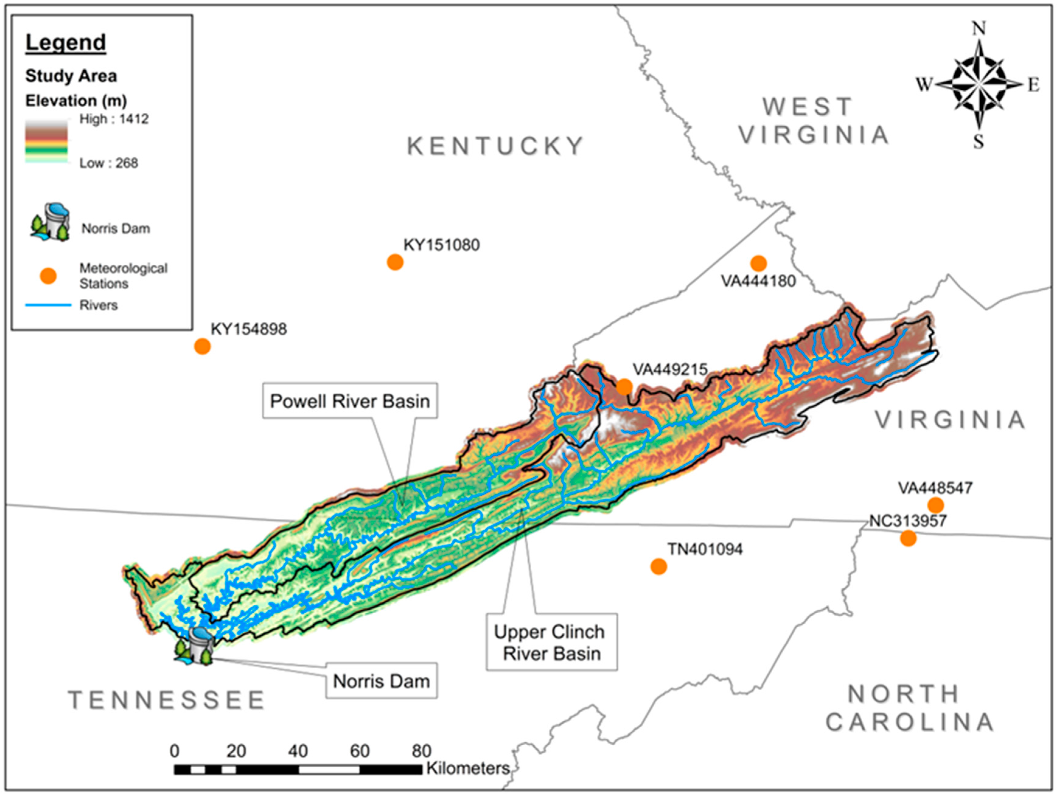
Figure 2.
Current Norris Reservoir Operating Guide. FG is the flood guide and BG is the balancing guide [34]. The shaded area is the 80 percent probability.
Figure 2.
Current Norris Reservoir Operating Guide. FG is the flood guide and BG is the balancing guide [34]. The shaded area is the 80 percent probability.
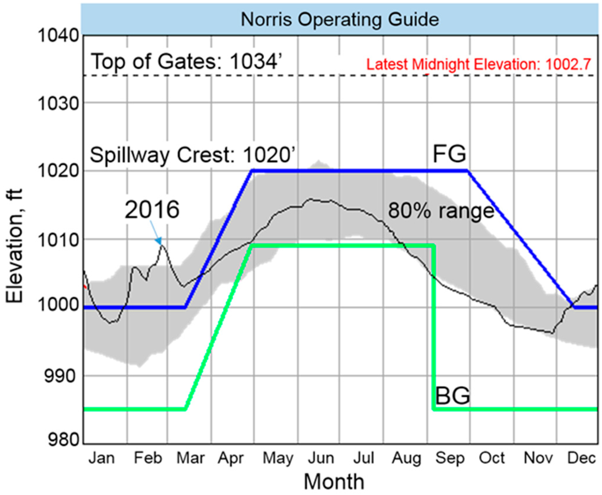
Figure 3.
Comparison of Observed (OBS) and “Base” reproduced by the Conditional Generation Method (CGM) for (a) precipitation and (b) temperature; “avg” and “std” indicates the average and standard deviation, respectively.
Figure 3.
Comparison of Observed (OBS) and “Base” reproduced by the Conditional Generation Method (CGM) for (a) precipitation and (b) temperature; “avg” and “std” indicates the average and standard deviation, respectively.

Figure 4.
Example comparison of hydrographs from 1985 to 1994 simulated by individual and combined hydrologic models with observed runoff.
Figure 4.
Example comparison of hydrographs from 1985 to 1994 simulated by individual and combined hydrologic models with observed runoff.
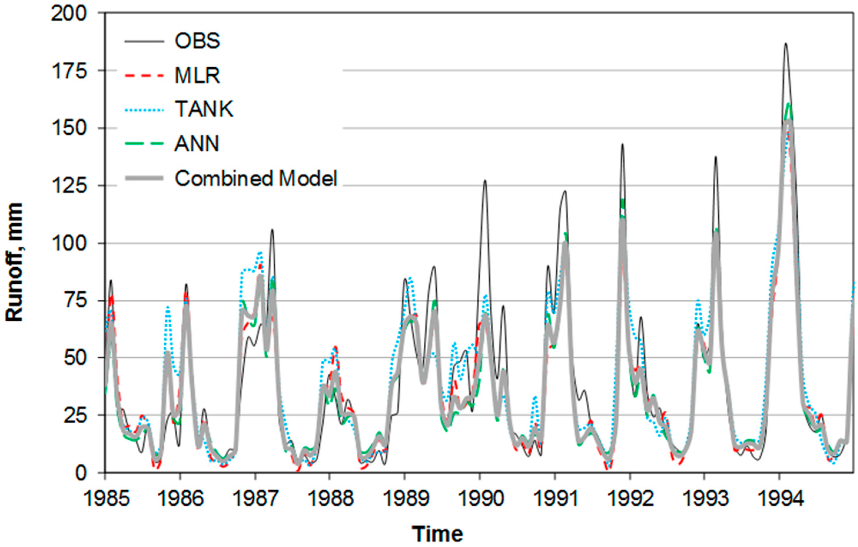
Figure 5.
Monthly runoff volume into Norris Reservoir for Base, 2020s, 2050s, and 2070s.
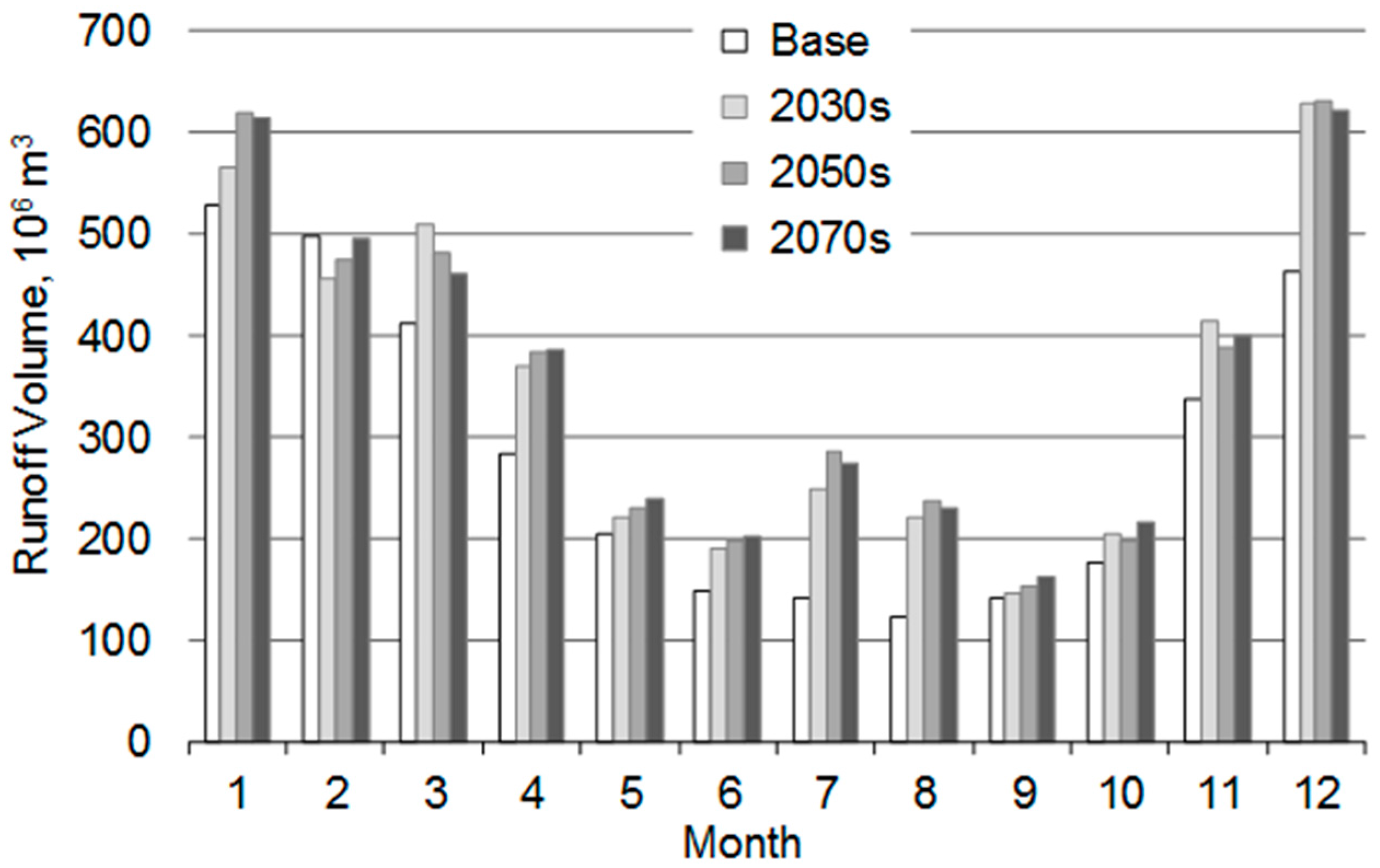
Figure 6.
Optimized operating guides compared to the current guide.


Table 1.
Penalty functions in Norris Dam operation.
| No. | Notation | Description | Violation | Note |
|---|---|---|---|---|
| Penalty Function (ft2) | ||||
| 0 | FG-BG | Elevation between the flood and balancing guides | 0 | Normal operation |
| 1 | FG | Elevation (EL) above the flood guide | (EL-FG)2 | Flood control |
| 2 | BG | Elevation below the balancing guide | (BG-EL)2 | Basic operation |
| 3 | HM | Elevation above the historical maximum 314.06 m (1030.38 ft) | 1000 | Flood control |
| 4 | NAV | Elevation below 219.08 m (955 ft) | 1000 | Navigation |
| 5 | TG | Elevation above 315.16 m (1034 ft) (top of gates) | 10,000 | Dam stability |
| 6 | COOL | Failure to provide cooling requirement flows for Bull Run Fossil Plant (seasonally 46 MCM~114 MCM per month) | 1000 | Service |
| 7 | ECOPOW | Failure to provide requirements for ecosystem and hydropower generation (19.96 MCM per month) | 10,000 | Ecology and hydropower |
| 8 | FLD | Flow exceeding maximum flow causing inundation (1028 MCM per month) | 10,000 | Flood control |
Table 2.
Performance comparison of the individual models and combined hydrologic models to observed runoff.
Table 2.
Performance comparison of the individual models and combined hydrologic models to observed runoff.
| Test | Equation | MLR | TANK | ANN | Combined Model |
|---|---|---|---|---|---|
| R2 (t = 1~m months) | 0.75 | 0.73 | 0.81 * | 0.81 | |
| Mean Absolute Error (MAE) (mm) (m = number of months) | 12.22 | 13.66 | 11.00 * | 11.04 | |
| Annual Runoff MAE (mm) (n = number of years) | 19.49 * | 37.16 | 28.54 | 20.55 | |
| High Flow Season MAE (mm) (i = November~April) | 3.44 * | 4.93 | 4.91 | 3.67 | |
| Low Flow Season MAE (mm) (i = May~October) | 0.19 | 1.25 | 0.15 * | 0.25 | |
| Low Runoff MAE (mm) (OBS < 10th percentile) | 4.47 * | 5.05 | 5.33 | 4.21 | |
| High Runoff MAE (mm) (OBS > 90th percentile) | 35.95 | 28.22 * | 28.57 | 30.50 | |
| 25–75th Quartile MAE (mm) (OBS inside interquartile) | 10.38 | 13.91 | 8.93 * | 9.22 |
Notes: Asterisks represent best performance among the three individual models. Bold values performed best by the Combined Model. Underlined Combined-Model values did not outperform at least two individual models. MLR: multiple linear regression; TANK: conceptual-water-balance model; ANN: artificial neural network; OBS: observed runoff; Model: modeled runoff; , , : number of months for OBS values less than 10th percentile, larger than 90th percentile, and inside the interquartile range, respectively.
Table 3.
Comparison of individual cumulative penalties for different time spans.
| Time Span | Operating Guide Scenarios | 1 | 2 | 3 | 4 | 5 | 6 | 7 | 8 | Sum |
|---|---|---|---|---|---|---|---|---|---|---|
| FG | BG | HM | NAV | TG | COOL | ECOPOW | FLD | |||
| Base | Current | 12,452 | 35,670 | 0 | 0 | 0 | 5460 | 0 | 0 | 53,582 |
| Base-Opt | 6497 | 29,610 | 0 | 0 | 0 | 5460 | 0 | 0 | 41,567 | |
| GCM-Opt | 6497 | 29,610 | 0 | 0 | 0 | 5460 | 0 | 0 | 41,567 | |
| 2030s | Current | 10,512 | 22,120 | 0 | 0 | 0 | 6450 | 0 | 6700 | 45,782 |
| Base-Opt | 5047 | 16,940 | 0 | 0 | 0 | 6450 | 0 | 6700 | 35,137 | |
| 2030-Opt | 4349 | 12,060 | 0 | 0 | 0 | 6450 | 0 | 6700 | 29,559 | |
| 2050s | Current | 10,280 | 20,880 | 0 | 0 | 0 | 7150 | 0 | 7000 | 45,310 |
| Base-Opt | 4961 | 16,130 | 0 | 0 | 0 | 7150 | 0 | 7000 | 35,241 | |
| 2050-Opt | 3662 | 11,810 | 0 | 0 | 0 | 7150 | 0 | 7000 | 29,622 | |
| 2070s | Current | 10,095 | 19,770 | 0 | 0 | 0 | 6220 | 0 | 3400 | 39,485 |
| Base-Opt | 4863 | 15,350 | 0 | 0 | 0 | 6220 | 0 | 3400 | 29,833 | |
| 2070-Opt | 3757 | 11,500 | 0 | 0 | 0 | 6220 | 0 | 3400 | 24,877 |
Table 4.
Percent changes in penalty of optimized operating guides compared to the current operating guide.
Table 4.
Percent changes in penalty of optimized operating guides compared to the current operating guide.
| Time Span | ∆ Penalty from Current when Using Base-Opt (%) | ∆ Penalty from Current When Using GCM-Opt (%) |
|---|---|---|
| Base | −22.4 | −22.4 |
| 2030s | −23.3 | −35.4 |
| 2050s | −22.2 | −34.6 |
| 2070s | −24.4 | −37.0 |
© 2017 by the authors. Licensee MDPI, Basel, Switzerland. This article is an open access article distributed under the terms and conditions of the Creative Commons Attribution (CC BY) license (http://creativecommons.org/licenses/by/4.0/).
Share and Cite
MDPI and ACS Style
Rungee, J.; Kim, U. Long-Term Assessment of Climate Change Impacts on Tennessee Valley Authority Reservoir Operations: Norris Dam. Water 2017, 9, 649. https://doi.org/10.3390/w9090649
AMA Style
Rungee J, Kim U. Long-Term Assessment of Climate Change Impacts on Tennessee Valley Authority Reservoir Operations: Norris Dam. Water. 2017; 9(9):649. https://doi.org/10.3390/w9090649
Chicago/Turabian StyleRungee, Joseph, and Ungtae Kim. 2017. "Long-Term Assessment of Climate Change Impacts on Tennessee Valley Authority Reservoir Operations: Norris Dam" Water 9, no. 9: 649. https://doi.org/10.3390/w9090649
Note that from the first issue of 2016, this journal uses article numbers instead of page numbers. See further details here.