Coupling the Modified Linear Spectral Mixture Analysis and Pixel-Swapping Methods for Improving Subpixel Water Mapping: Application to the Pearl River Delta, China

Abstract

High-resolution water mapping with remotely sensed data is essential to monitoring of rainstorm waterlogging and flood disasters. In this study, a modified linear spectral mixture analysis (LSMA) method is proposed to extract high-precision water fraction maps. In the modified LSMA, the pure water and mixed water-land pixels, which are extracted by the Otsu method and a morphological dilation operation, are used to improve the accuracy of water fractions. The modified LSMA is applied to the 18 October 2015 Landsat 8 OLI image of the Pearl River Delta for the extraction of water fractions. Based on the water fraction maps, a modified subpixel mapping method (MSWM) based on a pixel-swapping algorithm is proposed for obtaining the spatial distribution information of water at subpixel scale. The MSWM includes two steps in subpixel water mapping. The MSWM considers the inter-subpixel/pixel and intra-subpixel/subpixel spatial attractions. Subpixel water mapping is first implemented with the inter-subpixel/pixel spatial attractions, which are estimated using the distance between a given subpixel and its surrounding pixels and the water fractions of the surrounding pixels. Based on the initialized subpixel water mapping results, the final subpixel water maps are determined by a modified pixel-swapping algorithm, in which the intra-subpixel/subpixel spatial attractions are estimated using the initialized subpixel water maps and an inverse-distance weighted function of the current subpixel at the centre of a moving window with its surrounding subpixels within the window. The subpixel water mapping performance of the MSWM is compared with that of subpixel mapping for linear objects (SPM_L) and that of the subpixel/pixel spatial attraction model (SPSAM) using the GF-1 reference image from 20 October 2015. The experimental results show that the MSWM shows better subpixel water mapping performance and obtains more details than SPM_L and SPSAM, as it has the largest overall accuracy values and Kappa coefficients. Furthermore, the MSWM can significantly eliminate the phenomenon of jagged edges and has smooth continuous edges.

1. Introduction

Areas of impervious surface have significantly increased along with the rapid urbanization, leading to a rapid decrease in areas of forest, farmland, wetland, and river floodplain [1]. The areas of forest, farmland, wetland, and river floodplain can act as a sponge for storing water and regulating runoff, which are important for reduction, mitigation, and prevention of rainstorm waterlogging and flood disasters. The Pearl River Delta (PRD) is frequently struck by heavy rainstorms, which often results in urban waterlogging [2]. Therefore, accurate land surface water mapping at higher resolutions is very relevant.

As an effective mapping method for extracting surface water, subpixel mapping (SPM), or super-resolution mapping, was first introduced by Atkinson [3] to retrieve an appropriate spatial distribution for land cover fractions within each pixel. SPM can be considered a post-processing technique that combines the advanced features of both hard and soft classifications based on the spatial dependence theory [3]. Various SPM methods have been developed and grouped into two categories according to whether prior spatial structure information is required. The SPM methods in the first category do not necessarily require prior spatial structure information of land cover classes and are mainly based on spatial dependence. These SPM methods contain linear optimization techniques [4], pixel-swapping algorithms [5,6,7,8], subpixel/pixel spatial attraction models (SPSAM) [9,10,11,12], Markov random fields [13,14,15], Hopfield neural networks [16,17,18,19] and Swarm Intelligence Theory [16,17,18,19]. The SPM methods in the second category, which do need prior information from available high spatial resolution images, include the back-propagation neural network [20,21], two-point histogram [22], and indicator cokriging [23,24,25]. The aforementioned SPM methods have been successfully applied to map subpixel land cover and have an acceptable accuracy in subpixel mapping. For mapping the waterline or shoreline at a subpixel scale, many relevant SPM methods have been continuously developed [26,27]. Muslim et al. [28] used the pixel-swapping algorithm to accurately map the shoreline, combining with a localized soft classification approach. Foddy et al. [29] evaluated the super-resolution mapping methods to map the waterline at a subpixel scale. The results showed that the geostatistical approach can make the most accurate predictions of waterline location. Ling et al. [30] presented a novel algorithm based on a high spatial resolution digital elevation model (DEM) to map the subpixel-scale waterline according to the physical features of the water flow and additional information provided by the DEM. Zhang and Chen [31] proposed a super-resolution mapping technique based on geostatistics to extract coastline at a subpixel scale using the fine-resolution indicator variogram as the prior model of spatial structure. Ge et al. [32] proposed a linear template matching-based SPM algorithm (SPM_L) to predict the spatial distribution of linear objects, including water and roads. The experimental results demonstrated that the proposed SPM performed better than traditional SPM methods in mapping linear objects. However, the mapping accuracy of these subpixel mapping methods was highly dependent on the accuracy of water or land cover fractions of the linear spectral mixture analysis (LSMA) [33].

The endmember class fractions can be quantitatively extracted from remote sensing images using the conventional LSMA method, which decomposes the reflectance of a mixed pixel into different proportions [33]. This method has been successfully applied for extracting impervious surface, vegetation, soil, and water fractions. However, the LSMA involving all of the land-cover types was too complicated for only mapping surface water [34]. Previous studies have proposed modified methods for subpixel water mapping [35,36]. Ma et al. [37] proposed a locally adaptive unmixing method to extract lake-water area using 250 m MODIS images, which referred to the reflectivity of the neighbouring pixels with different weights. Xie et al. [34] proposed an adaptive iterative endmember class selection method based on the spatial similarity of adjacent ground surfaces for automated subpixel surface water mapping from a Landsat 8 OLI image. Pardopascual et al. [38] presented a high precision geometric method for automated shoreline detection from Landsat TM and ETM+ imagery. The above experiments showed that these methods can obtain better performance in water mapping than the conventional LSMA. However, the greatest spectral similarity of endmembers within each pixel constrains the prediction of inter-class boundaries among pixels, which still leads to certain difficulty in the accurate extraction of water fractions with subpixel precision [29,39]. To extract high-precision endmember class fractions, a modified LSMA method was developed by integrating spectral indices, including the normalized difference built-up index, the normalized difference bare-soil index, and the normalized difference vegetation index [2,40]. High-precision surface water fractions are required to map the spatial distribution of water at a subpixel scale, which determines the precision of subpixel water mapping. However, the LSMA method cannot retrieve the spatial distribution for surface water fractions at a subpixel scale. The appropriate spatial distribution for surface water fractions within each pixel can be obtained by the SPM methods.

In this study, we propose a modified LSMA method to extract the water fractions in five regions of PRD, China, by combining a high-resolution image from GF-1 and the pure water and mixed water-land pixels. The high-precision water fractions can be then integrated into a modified pixel-swapping algorithm to estimate subpixel-scale water bodies. The goal of this study is to improve the extraction accuracy of water at a subpixel scale, mainly for river-water, which includes: (1) extracting the pure water and mixed water-land pixels with a normalized difference water index (NDWI) using the Otsu method and a morphological dilation operation; (2) modifying the conventional LSMA with the pure water and mixed water-land pixels to extract the high-quality water fractions of each pixel; and (3) proposing a modified subpixel water mapping method (MSWM) based on the pixel-swapping algorithm to extract water bodies at a subpixel scale based on the unmixing water fractions of the modified LSMA.

2. Study Area and Data

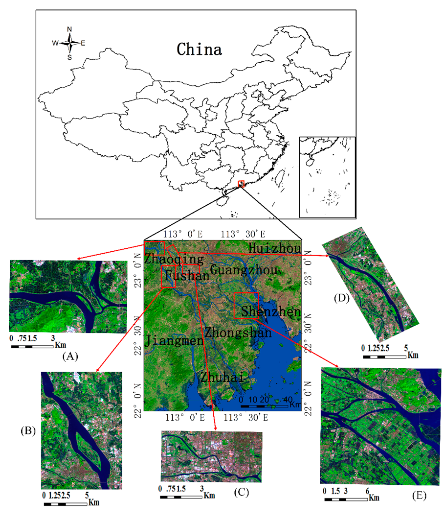
2.1. Study Area

The PRD region locates in Guangdong Province in southern China (Figure 1), and contains nine large prefectural cities: Guangzhou, Shenzhen, Foshan, Dongguan, Zhongshan, Zhuhai, Huizhou, Jiangmen, and Zhaoqing. It is a typical subtropical monsoon climate, with an annual average temperature of 21.0–23.0 °C. The rainy season is from April to September, and the dry season is from October to March [41]. The annual average precipitation in the PRD is about 1600 mm over 130 rainy days per year, which contributes to the high river levels. The water bodies in this region are very diverse. To extract different surface water bodies with remote sensing imagery, five regions with different land use types are selected as the case study areas in Figure 1.

2.2. Remote Sensing Image

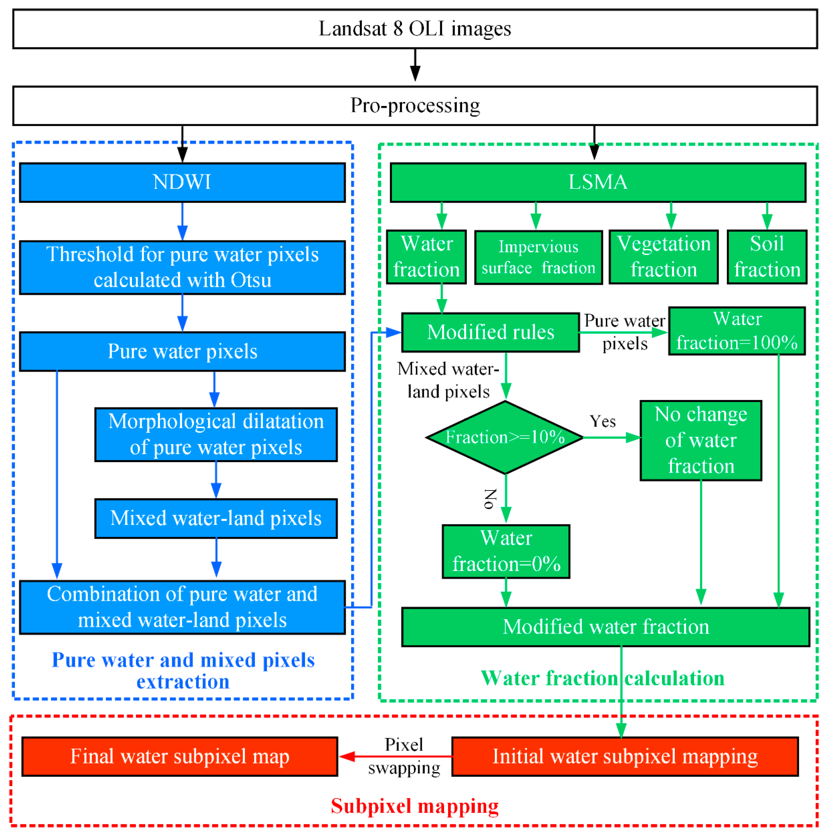
In this study, we used the Landsat-8 Operational Land Imager (OLI) without cloud cover (Acquired on 18 October 2015) for mapping the subpixel surface river water from heterogeneous environment. We obtained a pre-processed dataset or a raw dataset from the United States Geological Survey (USGS) Landsat distribution scheme (https://landsat.usgs.gov/landsat-surface-reflectance-high-level-data-products). In this study, the pre-processed Landsat-8 surface reflectance data, which were generated from the L8SR algorithm [42], were downloaded from the USGS Earth Resources Observation and Science (EROS) Center Science Processing Architecture (ESPA) on Demand Interface (https://espa.cr.usgs.gov/). The surface reflectance products were geometrically rectified to the Universal Transverse Mercator (UTM) projection system (zone 49N). In addition, to verify the accuracy of subpixel water mapping, a reference image with a spatial resolution of 6 m was obtained with a geometrically-corrected fusion GF-1 image from 20 October 2015. The fusion GF-1 image was generated by fusing multi-spectral data and panchromatic data from the GF-1 image via the Gram–Schmidt method [43,44,45]. The Gram–Schmidt method showed good performance in GF-1 image fusion because it can preserve the original spectral characteristics and reduce the loss of useful information [46,47].

3. Methods

The subpixel water mapping method (SWMM) was divided into three major steps: (1) extracting the pure water and land-water pixels automatically (Section 3.1); (2) extracting the fraction map of water bodies using the linear spectral mixture analysis method and modifying the fraction of water bodies by combining the pure water pixels (Section 3.2); and (3) achieving the fine spatial resolution water maps based on a modified subpixel water mapping method (MSWM). The detailed process of the SWMM method is shown in Figure 2.

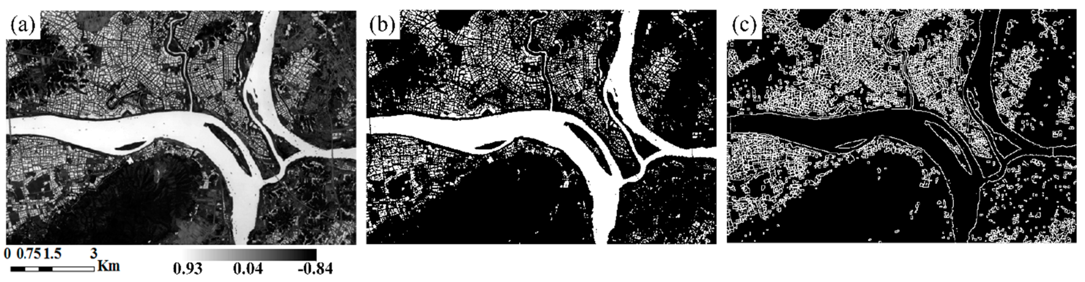
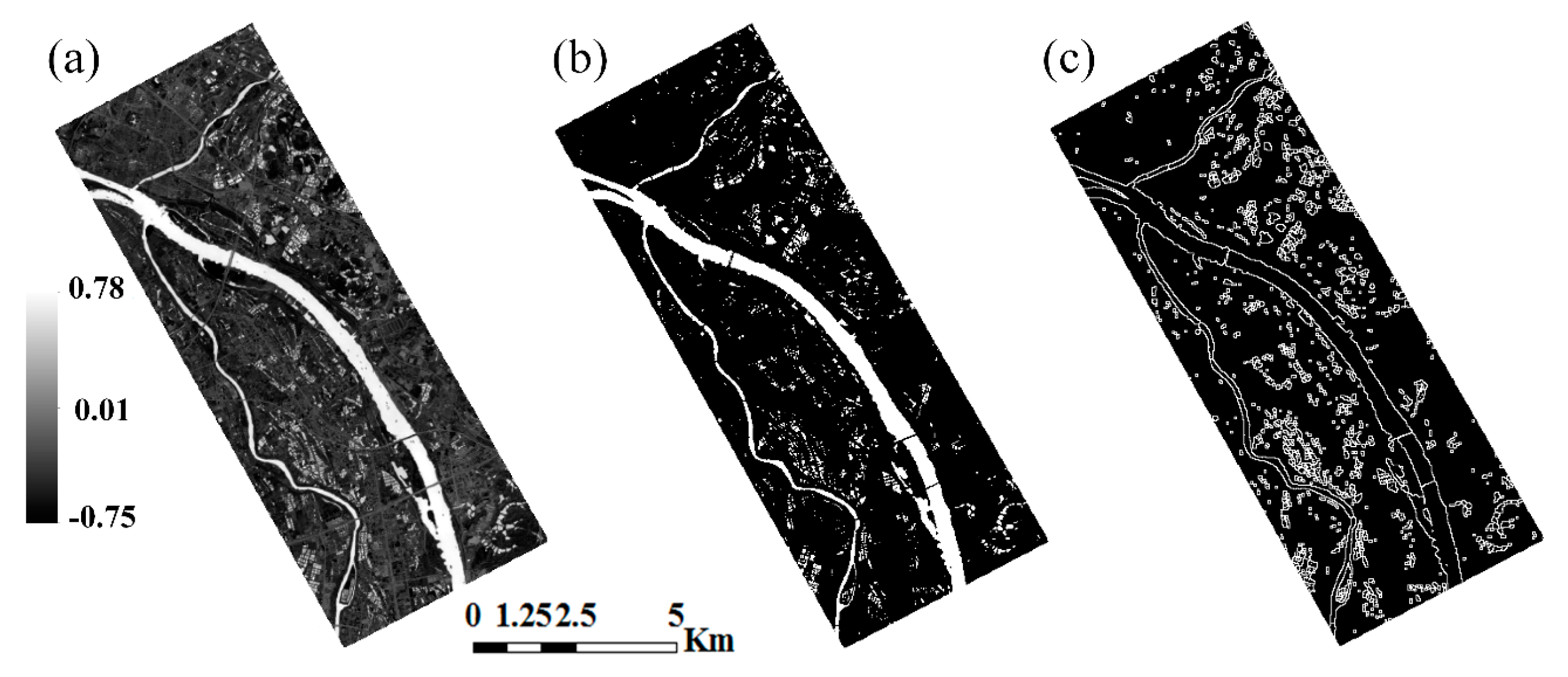
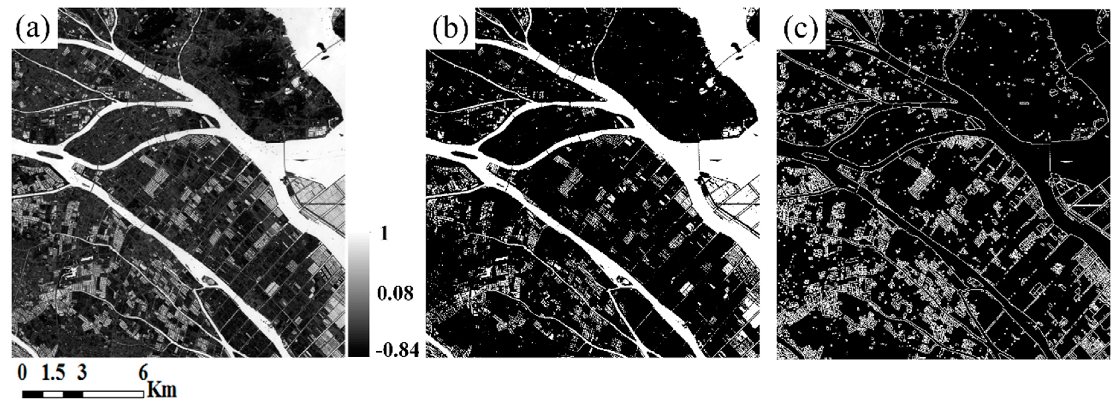
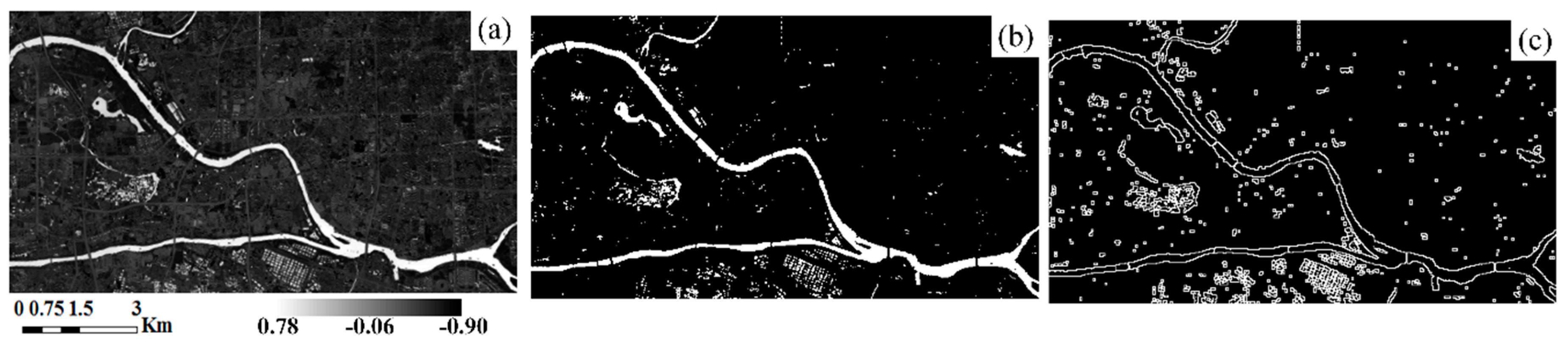
3.1. Automatic Extraction of Pure and Mixed Pixels

The NDWI has been widely used to extract land surface water (LSW) because of its unique characteristic of more accurately delineating LSW information from remote sensing imagery [48,49]. A previous study demonstrated that the NDWI using the green band (Band 3) and short-wave infrared band 1 (SWIR1, Band 6) of Landsat 8 OLI imagery shows better performance in accurately mapping LSW [50].

$$NDWI=\frac{{\rho }_{Green}-{\rho }_{SWIR1}}{{\rho }_{Green}+{\rho }_{SWIR1}}$$

(1)

where ${\rho }_{Green}$ and ${\rho }_{SWIR1}$ are the reflectances of band 3 and band 6, respectively.

In this study, based on the NDWI, the pure water and mixed water-land pixels are identified using the threshold and morphological dilatation methods, respectively. In general, the pure water pixels are extracted by setting the NDWI threshold value to 0 [48,49]. However, this threshold cannot be applied to every region because water in different regions shows different spectral features. The Otsu method [51] determines the optimal threshold through the maximum inter-class variance criterion and has been successfully utilized for extracting water and land pixels [34,52]. The mathematical formula of the Otsu method is as follows:

$$\{\begin{array}{c}{\sigma }^2=P_{nw}·{\left(M_{nw}-M\right)}^2+P_w·{\left(M_w-M\right)}^2\\ M=P_{nw}·M_{nw}+P_w·M_w\\ \begin{array}{c}{P}_{nw}+P_w=1\\ t=arg \underset{a\le t\le b}{\max }\left[P_w·P_{nw}·{\left(M_w-M_{nw}\right)}^2\right]\end{array}\end{array}$$

(2)

where $\sigma$ is the inter-class variance; M is the mean value of NDWI; $P_{nw}$ and $P_w$ are the percentage of non-water and water pixels, respectively; $M_{nw}$ and $M_w$ are the mean values of non-water and water pixels of NDWI, respectively; and t is the optimal threshold. The Otsu method is used to obtain the pure water pixels via application to the NDWI image. Here, the pure water pixels are extracted if the NDWI of a given pixel is greater than the threshold t.

A previous study demonstrated that the mixed water-land pixels between water and land are adjacent to and surround the pure water pixels, and they can be determined according to their spatial relationship to the pure water pixels [37]. In this study, based on their unique spatial relationship, the mixed water-land pixels are extracted by dilating the pure water pixels through a morphological dilation operation, with a window of size 3 $\times$ 3 pixels. If any one pixel in the window is adjacent to and surrounds a pure water pixel at the centre of the window, then the pixel is changed to a pure water pixel. If all pixels in the window are land or mixed pixels, then these pixels are not changed.

3.2. Modified Linear Spectral Mixture Analysis

In this study, the conventional linear spectral mixture analysis (LSMA) method [33] is used to extract the fractions of water, impervious surface, vegetation and soil endmembers, and the mathematical formula is as follows:

$$R_i={\displaystyle \sum }_{k=1}^n{f}_k{R}_{ik}+{\epsilon }_i$$

(3)

where R_i is the spectral reflectance of mixed pixels for band i, i = 1, 2, …, m; m is the number of spectral bands, k = 1, 2, …, n; n is the number of endmembers (here four endmembers are selected); f_k is the proportion of water, impervious surface, vegetation, and soil endmembers; R_ik is the known spectral reflectance of endmember k of band i; and ${\epsilon }_i$ is the error of band i. The proportion f_k of four endmembers is solved by the least square method with the following constraint:

$${\displaystyle \sum }_{k=1}^n{f}_k=1, f_k\ge 0$$

(4)

Endmember selection is a necessary prerequisite to spectral mixture analysis and is critical for accurately extracting the fraction of endmembers. However, large errors exist in the LSMA results, partly because some endmembers are misclassified during the process of endmember selection. Following the work of Xu et al. [2], a two-step method is applied to improve the accuracy of endmember selection by combining the Maximum Noise Fraction (MNF) and a high-resolution image from Google Earth. However, the numerical problems of LSMA and the imprecise selection of pure endmembers directly result in large errors in the LSMA results; for instance, some water endmember fractions in the pure water pixels may be misclassified as other endmembers. The inaccurate water fraction limits the accuracy of subpixel water mapping. In this study, the pure water pixels extracted by the Otsu algorithm and the mixed water-land pixels extracted by dilating the pure water pixels (Section 3.1) are used to modify the water fractions by setting an appropriate value based the above LSMA results. The detailed post-processing of the water fraction image is shown in Figure 2. In general, the water fraction of the pure water pixels is set to 100%. Some studies have shown that an error of approximately 10% still exists in the LSMA results [2,53]. Therefore, to reduce uncertainties introduced by LSMA, water fractions less than 10% in the mixed water-land pixels are set to 0, and these mixed water-land pixels are not used in subpixel water mapping.

3.3. Modified Subpixel Water Mapping Method

Based on the subpixel/pixel spatial attraction model in Mertens et al. [9] and the pixel-swapping algorithm [5,6], a modified subpixel water mapping method is proposed to predict the spatial distribution of water at a subpixel scale using the previous high-precision water fraction maps. The MSWM includes two steps for subpixel water mapping, which estimates the inter-subpixel/pixel and intra-subpixel/subpixel spatial attractions, respectively. This study is focused on subpixel water mapping; thus, only the water fractions of pixels are used, and the land fractions of pixels are set to 0.

In the initialized process of subpixel water mapping, the water spatial attraction of the current subpixel within a pixel is influenced by the water fractions in surrounding pixels, and is calculated as:

$$Inter{A}_{ij}={\displaystyle \sum }_{m=-2}^2{\displaystyle \sum }_{n=-2}^2\frac{Frac\left(x+m,y+n\right)}{d\left(p_{ij},P_{x+m,y+n}\right)} , i, j=1, 2,\cdots , S$$

(5)

where (x, y) are the coordinates of the current pixel, $Inter{A}_{ij}$ is the spatial attraction of the current subpixel for the water class, i and j are row and column indices of the subpixels with the pixel, respectively, and S is the scale factor. m and n are row and column indices of a window such that the current pixel (x, y) is at the centre of the window. The window size indicates the total number of surrounding pixels involved in the calculation of the inter-subpixel/pixel spatial attractions. Atkinson demonstrated that just one neighbour, being 3 window size, for subpixel mapping may produce unsatisfactory results, and the window size of 5 (two neighbours) may achieve high subpixel mapping accuracy [5]. Thus, in this study, m and n are both set to −2, −1, 0, 1, and 2, which means that 25 surrounding pixels are used to calculate the spatial attractions. $Frac\left(x+m,y+n\right)$ is the water fraction of the surrounding pixels $P_{x+m,y+n}$, and $d\left(p_{ij},P_{x+m,y+n}\right)$ is the distance between the current subpixel $p_{ij}$ and its surrounding pixels $P_{x+m,y+n}$. The distance can be calculated as:

$$d\left(p_{ij},P_{x+m,y+n}\right)= \sqrt{{\left(x_i^{\prime }-X_{x+m}^{\prime }\right)}^2+{\left(y_j^{\prime }-Y_{y+n}^{\prime }\right)}^2}$$

(6)

where ($x_i^{\prime }$, $y_j^{\prime }$) are the coordinates of subpixel $p_{ij}$; and ($X_{x+m}^{\prime }$, $Y_{y+n}^{\prime }$) are the coordinates of pixels $P_{x+m,y+n}$, which are calculated using:

$$\{\begin{array}{c}{x}_i^{\prime }=x+\frac{2\times i-1}{2\times S}\\ y_j^{\prime }=y+\frac{2\times j-1}{2\times S}\end{array} i,j=1, 2, \cdots , S$$

(7)

$$\{\begin{array}{c}{X}_{x+m}^{\prime }=x+m+0.5\\ Y_{y+n}^{\prime }=y+n+0.5\end{array} m,n=-2, -1, 0, 1, 2$$

(8)

After the spatial attractions of all the subpixels within pixel $P_{x,y}$ for the water class, the spatial attractions are sorted in descending order. According to the descending list of subpixels, the first $Frac\left(x,y\right) \times S^2$ subpixels in the list are allocated to the water class, other subpixels are allocated to the land class. $Frac\left(x,y\right) \times S^2$ determines the number of subpixels in pixel $P_{x,y}$ for the water class. The above processes are repeated until all subpixels of the water class within all pixels are allocated.

Once the initialized subpixel water allocation is completed, the subsequent subpixel water mapping is further improved based on the subpixel swapping method. The intra-subpixel/subpixel spatial attraction of the current subpixel at the centre of a moving window is influenced by the surrounding water class pixels within the window, and is calculated as:

$$Intra{A}_{ij}={\displaystyle \sum }_{m=-2}^2{\displaystyle \sum }_{n=-2}^2\lambda \left(p_{i,j},p_{i+m,j+n}\right)z\left(p_{i+m,j+n}\right)$$

(9)

where $Intra{A}_{ij}$ is the spatial attraction of the current subpixel $p_{i,j}$ for the water class, and $z\left(p_{i+m,j+n}\right)$ is the value of the subpixel $p_{i+m,j+n}$. $z\left(p_{i+m,j+n}\right)$ that is set to 1 for the water class, and 0 for the land class. In this study, the moving window size is set to 25, which indicates that 25 surrounding subpixels are used in the calculation of the intra-subpixel/subpixel spatial attraction. $\lambda \left(p_{i,j},p_{i+m,j+n}\right)$ is a distance-dependent weight:

$$\lambda \left(p_{i,j},p_{i+m,j+n}\right)=exp\left(\frac{-d\left(p_{i,j},p_{i+m,j+n}\right)}{\alpha }\right)$$

(10)

where $\alpha$ is a non-linear parameter of the exponential model, and $d\left(p_{i,j},p_{i+m,j+n}\right)$ is the distance between the current subpixel $p_{i,j}$ and its surrounding subpixels $p_{i+m,j+n}$, and calculated as:

$$d\left(p_{ij},p_{i+m,j+n}\right)=\sqrt{{\left(x_i^{\prime }-x_{i+m}^{\prime }\right)}^2+{\left(y_j^{\prime }-y_{j+n}^{\prime }\right)}^2}$$

(11)

Similarly, the spatial attraction for the land class is also calculated. After the intra-subpixel/subpixel spatial attractions of all the subpixels within pixel $P_{x,y}$ for the water and land classes are determined, the spatial attractions $IntraA$ are sorted in descending order. The list contains S² subpixels, which includes water and land classes. The water class is set to 1, and the land class is set to 0. In the list, the first “0” is found from left to right, and the first “1” is found from right to left. If the “0” is in front of the “1”, the class values are then swapped. Otherwise, no change is made. The above process is repeated iteratively until a solution is approached. The process can be stopped when further improvement cannot be obtained or the iterations reach a fixed number. The details of the subpixel-swapping algorithm can be found in Atkinson [5] and Wang [54].

4. Results and Discussion

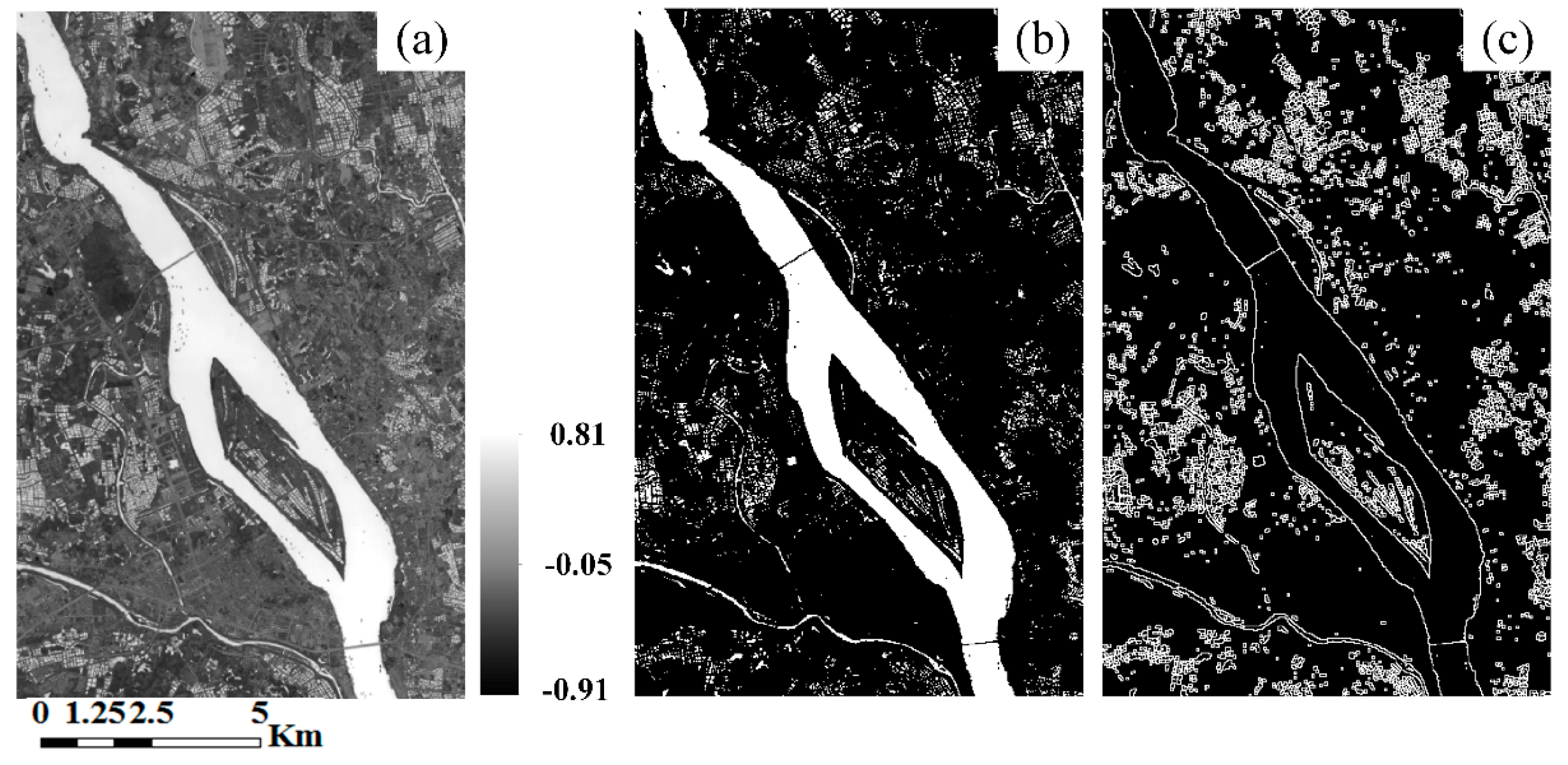
4.1. Extraction of Pure Water and Mixed Water-Land Pixels

This study explored the extraction of pure water and mixed water-land pixels using the NDWI. According to the histogram of NDWI, the thresholds of pure water were automatically estimated by the Otsu method. The thresholds of NDWI for the five study regions are 0.093, 0.114, 0.101, 0.053, and 0.171, which are different from the 0 threshold of Mcfeeters [48] and Xu [49]. The different water bodies of the five regions exhibit different spectral reflectance, leading to obviously different thresholds. The Otsu determined thresholds (Figure 3, Figure 4, Figure 5, Figure 6 and Figure 7) are applied to obtain five pure water maps by setting a condition such that the NDWI must be greater than the threshold. The pure water maps for the five regions are shown in subfigure b of Figure 3, Figure 4, Figure 5, Figure 6 and Figure 7. The visual interpretation indicates that the five pure water maps derived from the Otsu method show better performance than those pure water maps derived from a 0 threshold. The pure water maps derived from 0 threshold are not shown in this study. The mixed water-land pixels are determined through the dilation of the pure water pixels, as shown in subfigure c of Figure 3, Figure 4, Figure 5, Figure 6 and Figure 7.

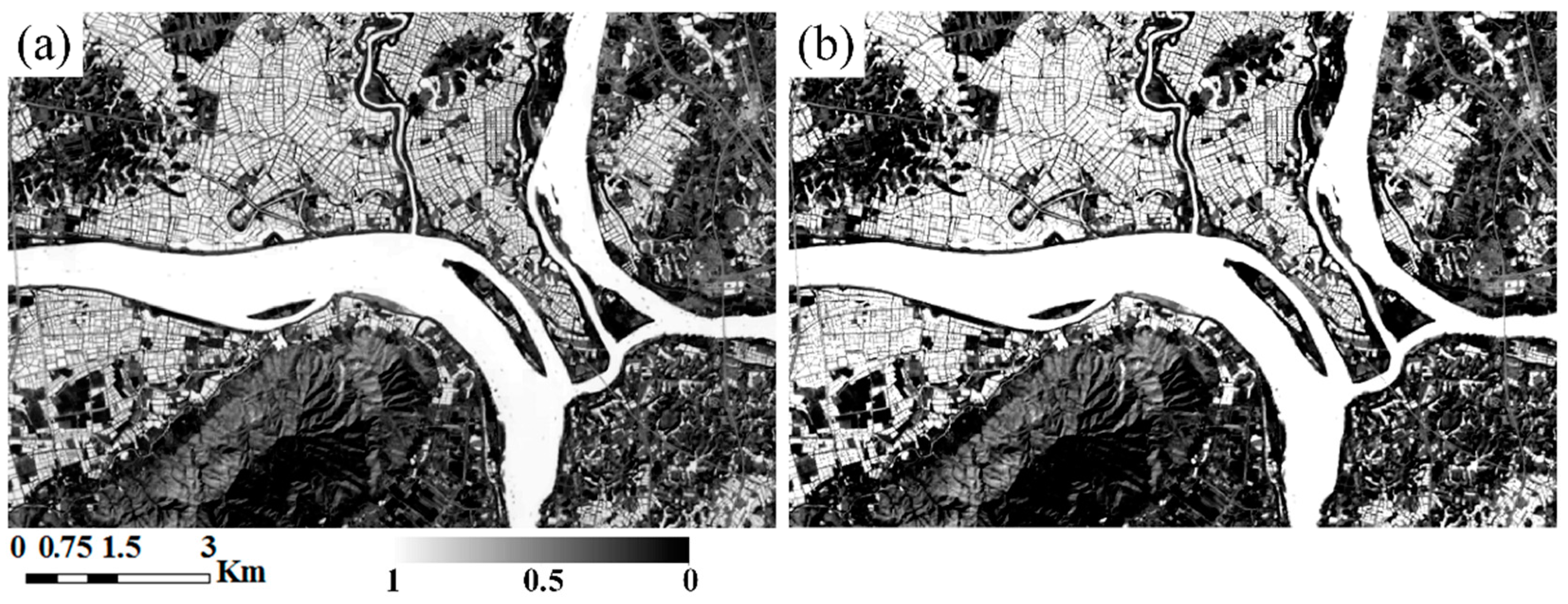
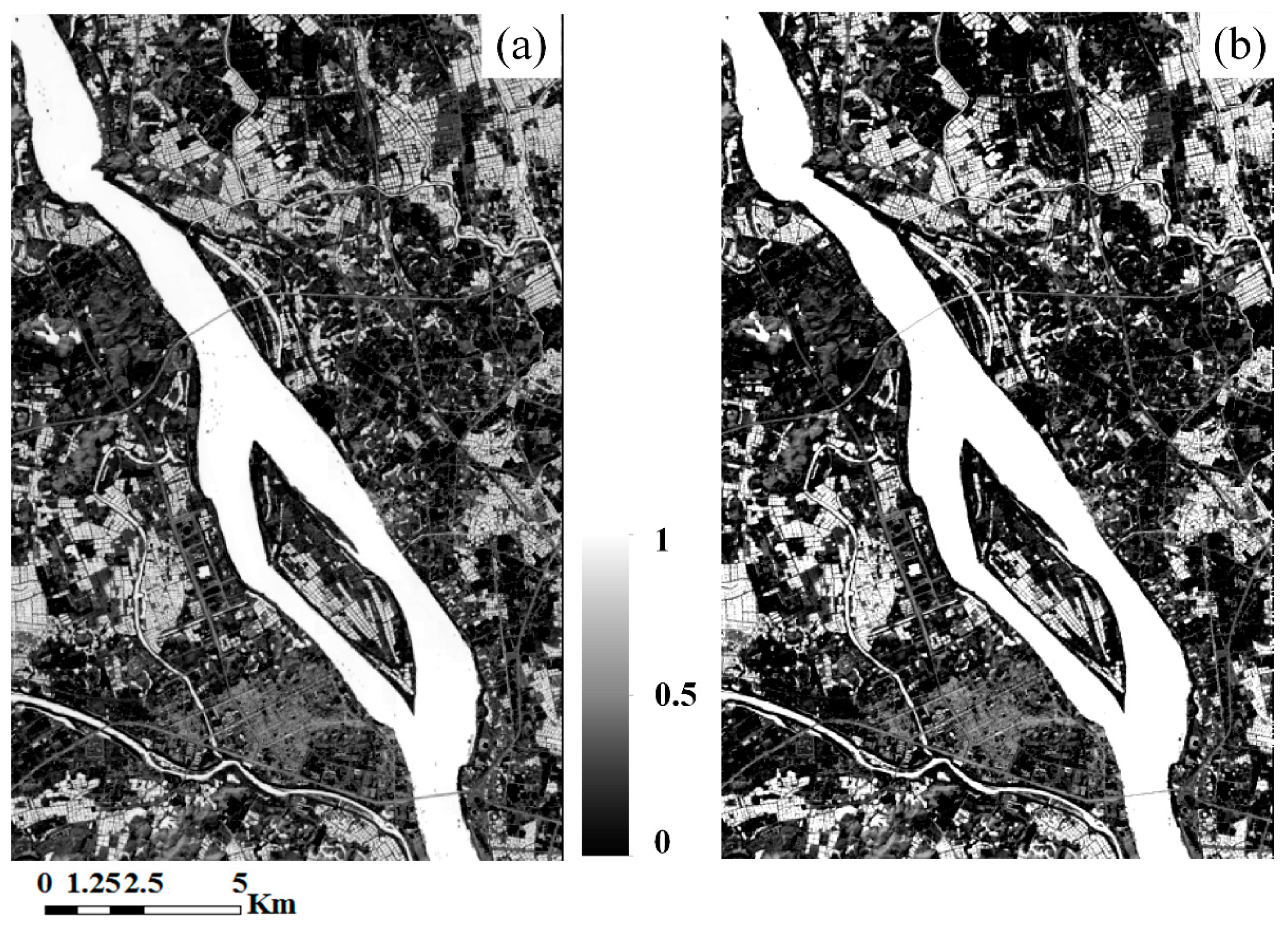
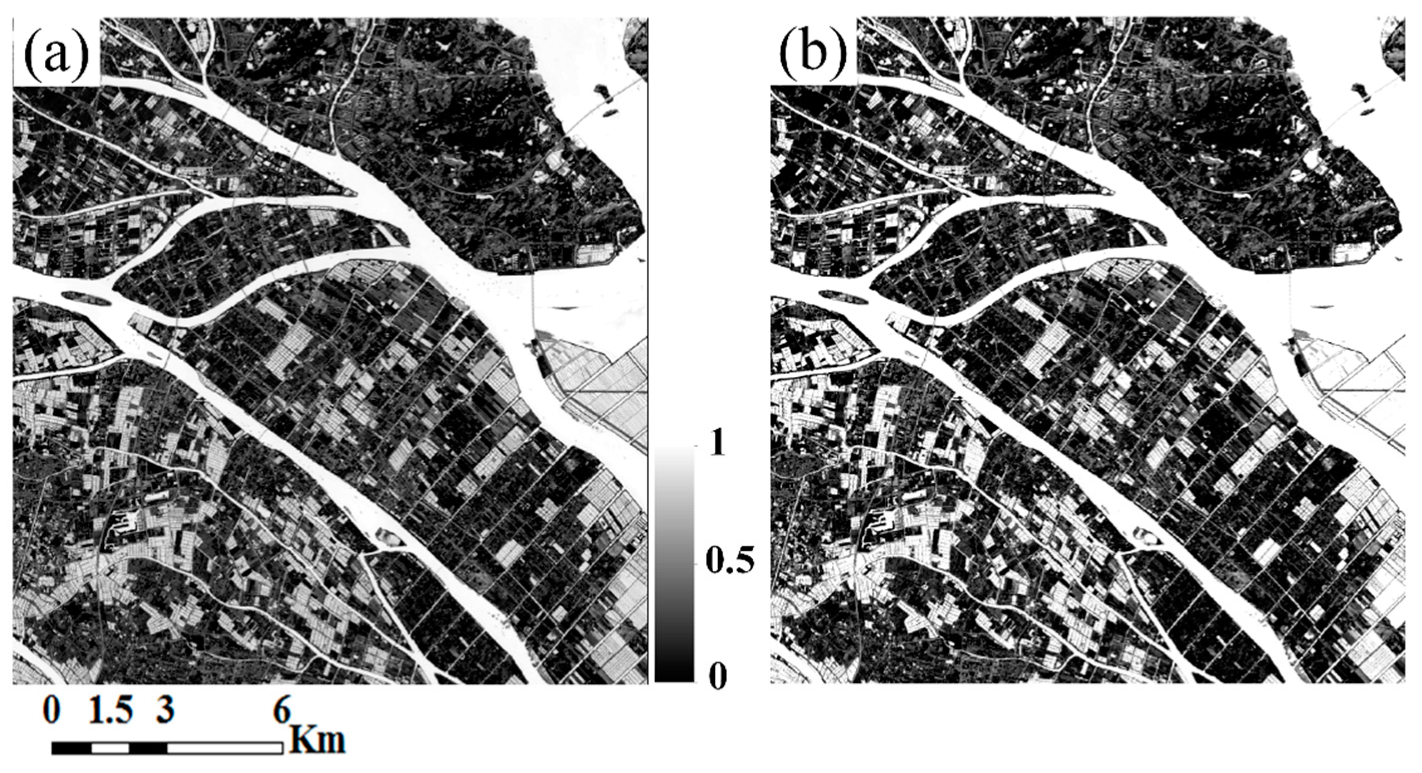
4.2. Extraction of Surface Water Fraction

In this study, the water, impervious surface, vegetation, and soil fractions were extracted by applying the conventional and modified LSMA methods using the Landsat 8 OLI image of 18 October 2015. The surface water fractions generated by the conventional and modified LSMA methods are shown in Figure 8, Figure 9, Figure 10, Figure 11 and Figure 12. It is obvious in Figure 8, Figure 9, Figure 10, Figure 11 and Figure 12 that the modified LSMA exhibits better extraction performance than the conventional LSMA, particularly for the pure water regions. For the conventional LSMA results, some pixels have a water fraction of less than 100% in the pure water pixels, which leads to large errors in the LSMA results. These results seem inconsistent to the actual situation. In general, the pure water pixels have a fraction of 100%. Large errors in the conventional LSMA results may be closely related to inaccurate endmember selection and accumulation errors in the least square equations. Furthermore, dredges and ships in the river may change the reflectance of the water body, such that these pixels may be mistakenly treated as mixed water-land or land pixels. This may also introduce errors to the water fractions determined by the conventional LSMA. Therefore, based on the NDWI, a modified LSMA method was proposed in this study. First, following the work of Xu et al. [2], accurate endmembers were selected by integrating a high-resolution image. Then, based on the LSMA results, the surface water fractions in the pure water pixels are modified by setting water fraction equal to 100%. As shown in subfigure b of Figure 8, Figure 9, Figure 10, Figure 11 and Figure 12, most pixels in the pure water regions have a water fraction of 100% in the modified LSMA.

The water fractions, especially those less than 10%, in the mixed water-land pixels are not improved in this study, which may reduce the accuracy of subpixel water mapping. Although some efforts have been made to improve the LSMA results, errors of about 10% can still be found. Water fraction less than 10% are set to 0% to reduce uncertainties due to the calculation error of LSMA. This means that mixed water-land pixels with water fraction less than 10% are involved in the subpixel mapping.

Furthermore, a bridge overlooking a river is considered land and has a water fraction of 0% (subfigure b in Figure 9, Figure 10 and Figure 11). These bridge pixels may break down the river into discrete partitions, which leads to boundary discontinuity in subpixel water mapping. This is contrary to the actual observation. In the future, we can further enhance the accuracy of LSMA by modifying the bridge pixels above surface water to be water pixels.

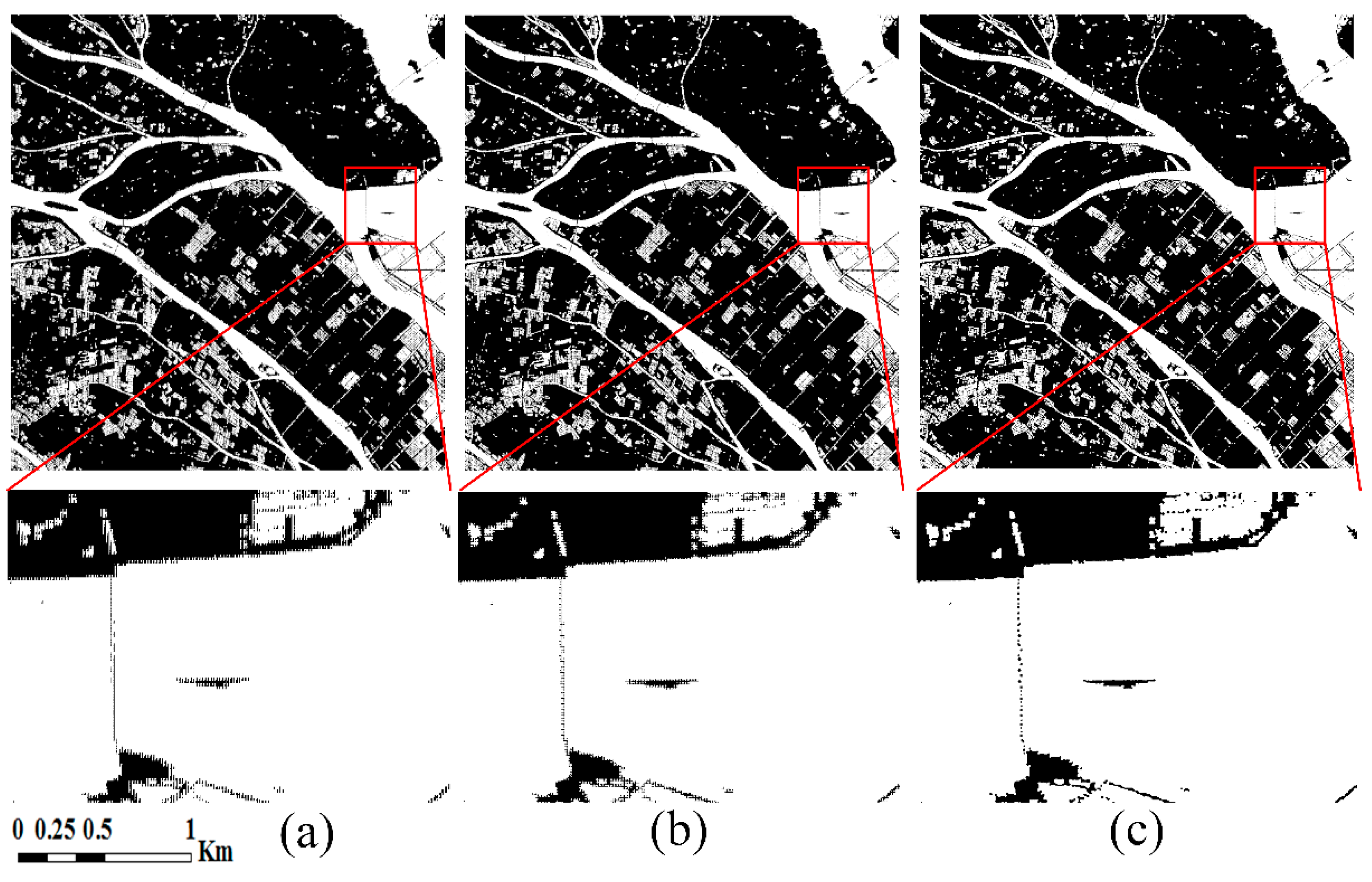
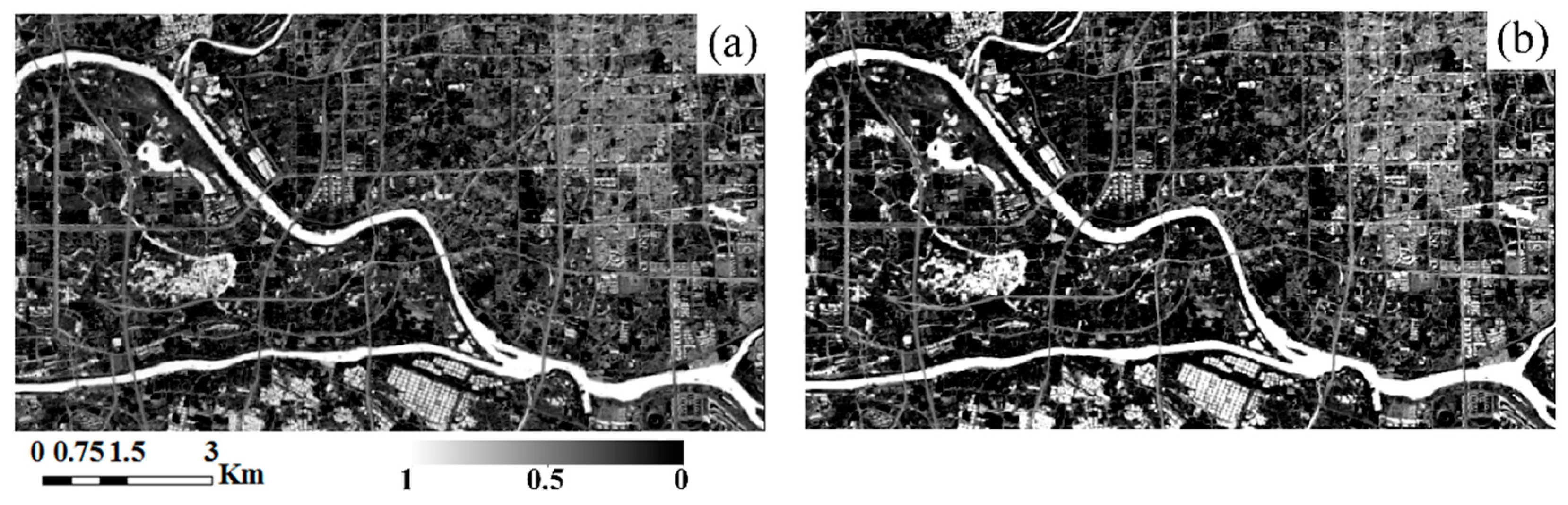
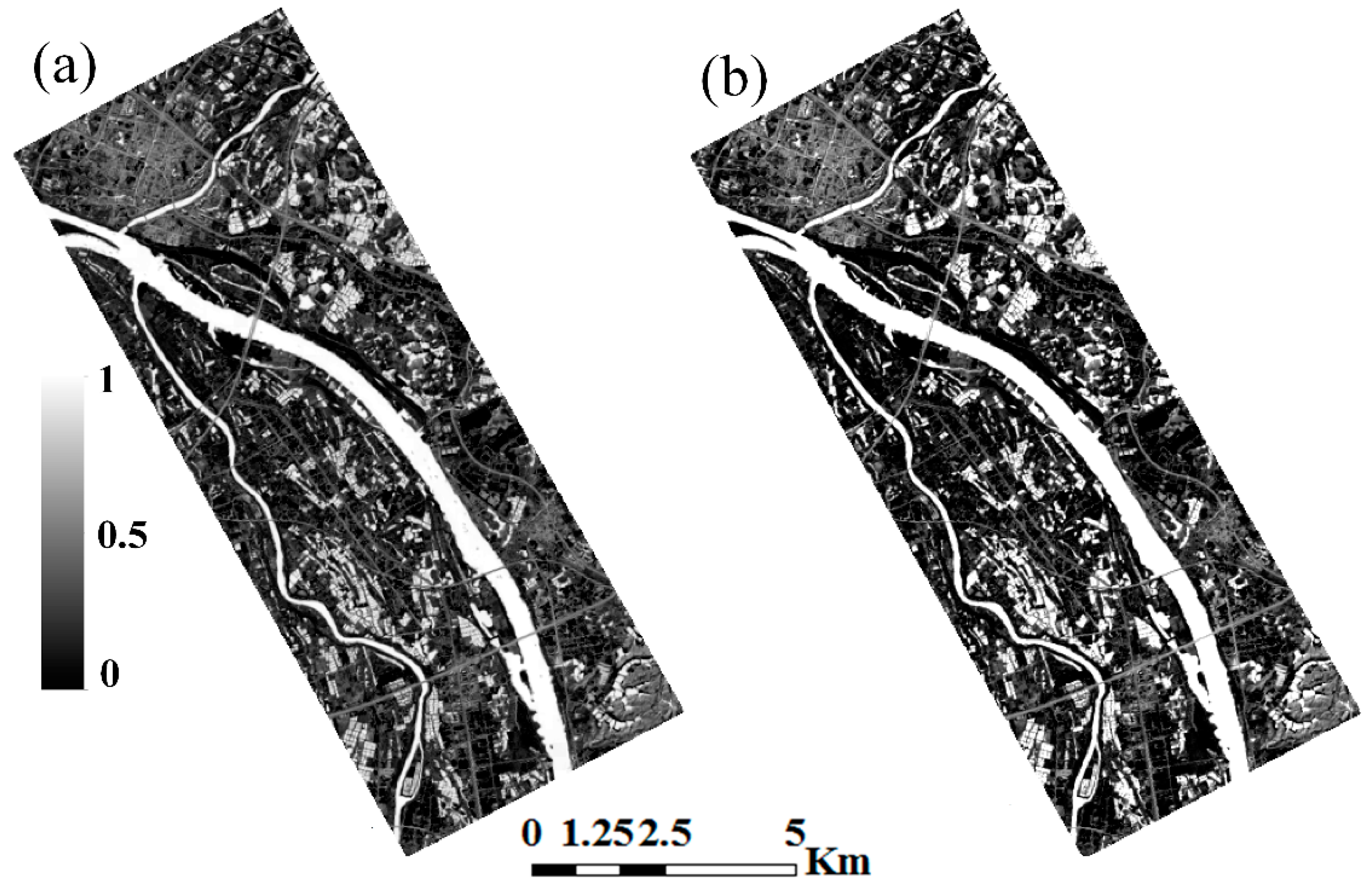
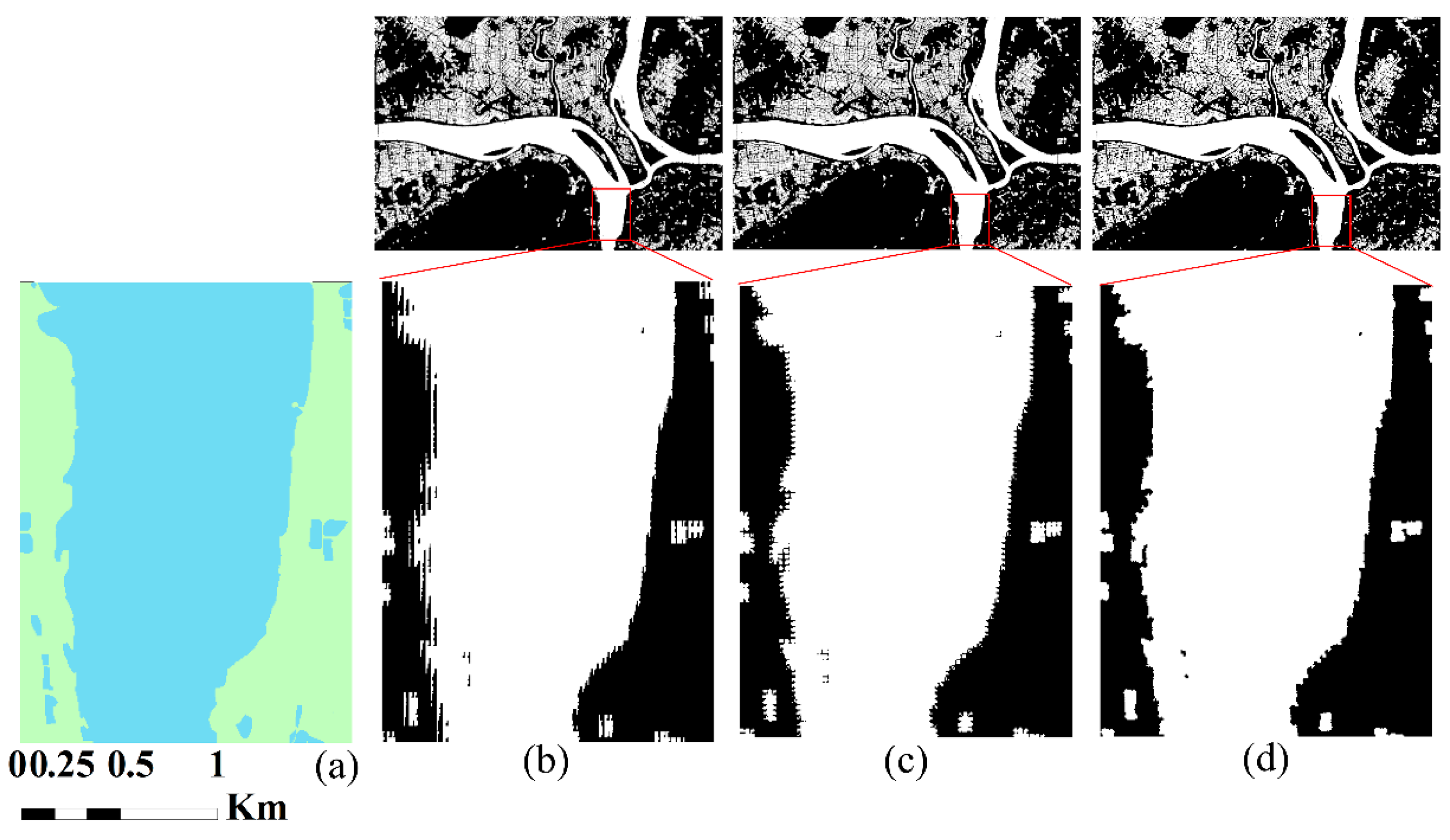
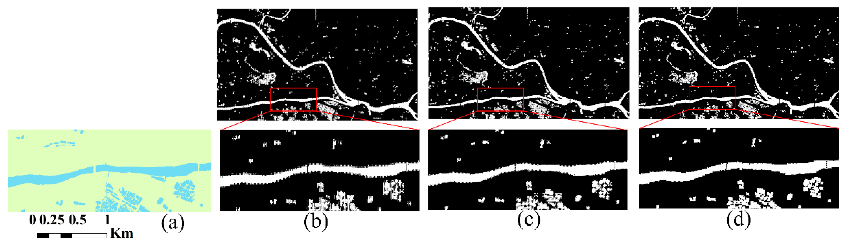
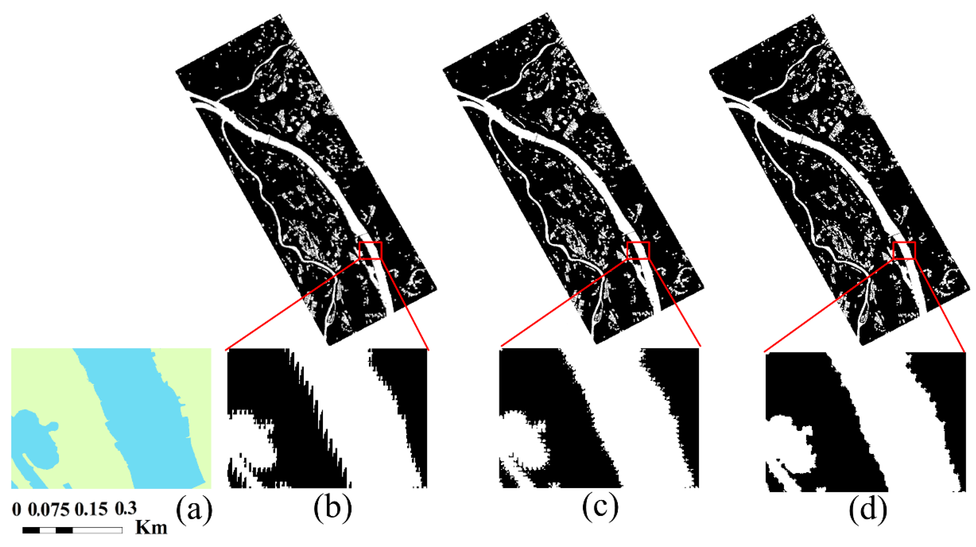
4.3. Comparison of Different Subpixel Water Mapping Methods

To verify the accuracy of subpixel water mapping, the fusion GF-1 image was first classified into water, vegetation, impervious surface, and soil by the maximum likelihood supervised classification method. Then, other classes except water were merged by a post-processing operation. After supervised classification, the water with a blue colour and land with a yellow-green colour were extracted, as shown in subfigure a of Figure 13, Figure 14, Figure 15 and Figure 16. Region E does not have a reference image because of the lack of a GF-1 image in the same period.

Furthermore, to validate the performance of the proposed MSWM method, this study compared the subpixel water mapping accuracies of the MSWM with those of SPM_L from Ge et al. [32] and SPSAM from Mertens et al. [9]. The MSWM, SPM_L, and SPSAM were coded with C# language, and the scale factor S was set to 5. Referring to the research of Atkinson [5], the non-linear parameter of the exponential model a and the moving window size were set to 5 pixels, and the number of iterations was 30 in the MSWM experiment. It should be noted that only the mixed water-land pixels surrounding the pure water pixels need to be mapped.

Figure 13, Figure 14, Figure 15, Figure 16 and Figure 17 show the subpixel water mapping results from the SPM_L, SPSAM, and MSWM experiments. The MSWM shows better mapping performance than the SPM_L and SPSAM for all regions. The SPM_L uses 20 rectilinear and curvilinear templates of 3 × 3 pixels to represent the direction of water inside mixed water-land pixels. The subpixel mapping results of SPM_L are closely associated with these templates, and have direction similar to the templates, as shown in subfigure b of Figure 13, Figure 14, Figure 15, Figure 16 and Figure 17. The optimal template is not shown here. The spatial dependence between subpixels and pixels of templates in four directions are taken into account. However, the SPM_L does not consider the spatial dependence between subpixels and neighbouring pixels acting towards template pixels. This may introduce large errors in subpixel mapping and yield a suboptimal subpixel mapping result (subfigure b in Figure 13, Figure 14, Figure 15, Figure 16 and Figure 17). In the SPSAM experiment, it is obviously demonstrated that some jagged edges exist at the junctions of water and land (subfigure c in Figure 13, Figure 14, Figure 15, Figure 16 and Figure 17). This may be attributed to imprecision of spatial dependence in the spatial attraction model. SPSAM only considers the spatial attraction between subpixels and pixels and does not consider the spatial attraction between subpixels and subpixels, which does not express the spatial dependence well. The MSWM can eliminate the phenomenon of jagged edges to some extents and has smooth continuous edges. Subfigure d in Figure 13, Figure 14, Figure 15, Figure 16 and Figure 17 also show that the subpixel water mapping results of the MSWM are most similar to the reference image. This is because the MSWM considers the inter-subpixel/pixel and intra-subpixel spatial dependence.

The subpixel mapping accuracies of SPM_L, SPSAM, and MSWM are further evaluated by calculating the Overall Accuracy (OA) and Kappa Coefficient (κ) with respect the reference image. The quantitative accuracy evaluation of subpixel mapping is shown in

Table 1. Comparisons of subpixel water mapping accuracy among MSMM, SPM_L, and SPSAM.

Region	Method	Whole Reference Image		Mixed Pixels in Reference Image
		Overall Accuracy (OA, %)	Kappa Coefficient (κ)	Overall Accuracy (OA, %)	Kappa Coefficient (κ)
A	MSWM	97.10%	0.94	80.89%	0.59
	SPML	96.46%	0.92	70.72%	0.42
	SPSAM	96.86%	0.93	77.39%	0.52
B	MSWM	95.35%	0.90	80.78%	0.60
	SPML	93.92%	0.87	65.97%	0.30
	SPSAM	94.85%	0.89	75.58%	0.50
C	MSWM	95.69%	0.84	76.23%	0.52
	SPML	94.18%	0.78	62.30%	0.24
	SPSAM	95.05%	0.82	70.30%	0.40
D	MSWM	97.24%	0.94	82.58%	0.60
	SPML	95.85%	0.92	70.96%	0.33
	SPSAM	96.78%	0.94	78.51%	0.50

. In Table 1, the MSWM OA values for Regions A and D are up to 97%, and κ reaches 0.94, which are higher values than those of SPM_L and SPSAM for the whole reference image. For the mixed water-land pixels in the reference image, the MSWM OA values are greater than 80% for Regions A, B, and D, while the largest OA value of SPM_L and SPSAM is only 78.51%; κ for Regions A, B, and D based on the MSWM are greater than 0.59, which is higher than that of SPM_L and SPSAM. The quantitative comparison analysis indicates that both the OA and κ values of the MSWM are the largest among the three subpixel mapping methods, and the MSWM exhibits better performance than SPM_L and SPSAM in subpixel water mapping.

From the visual and quantitative evaluation, it is concluded that the MSWM is more accurate for subpixel mapping than the other two subpixel mapping methods; the MSWM can obtain more details in subpixel mapping than SPM_L and SPSAM. However, some jagged edges can also be found in the MSWM results, as shown in Figure 16d. This may be related to the LSMA accuracy for mixed water-land pixels. The water fraction of each pixel in LSMA determines the number of subpixels in the pixels, which may directly influence the accuracy of subpixel mapping. Therefore, enhancing the accuracy of LSMA results is the primary task for improving the accuracy of subpixel mapping, especially for the water fraction of mixed pixels. A more reasonable LSMA could be exploited for extraction of water fraction by combining it with different normalized difference indices or different data in the future.

5. Conclusions

This study presents an improved method for surface water mapping with subpixel precision. In the proposed method, the pure water and mixed water-land pixels were first automatically extracted from the 18 October 2015 Landsat 8 OLI image based on NDWI using the Otsu method and a morphological dilation operation. A modified LSMA method was then built based on the conventional LSMA by combining a high-resolution image and the pure water and mixed water-land pixels; this method was used to extract water fractions. The modified LSMA performs better than the conventional LSMA in improving the water fraction of pure water pixels. As the water fractions for different regions were extracted in advance, a modified subpixel mapping method (MSWM) based on the pixel-swapping algorithm was proposed for subpixel water mapping. In the MSWM, the primary subpixel water mapping was first implemented by computing the spatial attraction between the current subpixel and the surrounding pixels within a window; the final subpixel water mapping was then obtained by estimating the spatial attraction between the current subpixel at the centre of a moving window and all surrounding subpixels within the window. In other words, the MSWM considers the inter-subpixel/pixel and intra-subpixel spatial attractions. In this study, three subpixel water mapping experiments were performed for five regions using the MSWM, SPM_L, and SPSAM methods. The subpixel mapping results were validated using the GF-1 reference image from 20 October 2015. The experimental results indicate that the MSWM indicates better performance and obtains more details in subpixel mapping than SPM_L and SPSAM, as it has the largest overall accuracy values and Kappa coefficients. Furthermore, the MSWM can significantly eliminate the phenomenon of jagged edges and has smooth continuous edges. Overall, the MSWM is an effective subpixel mapping method, which can improve subpixel mapping accuracy. However, the proposed method does not work fine in these water bodies with dredges, ships, suspended sediment load, and floating vegetation. These pixels may change the reflectance of water, which may be mistakenly considered as land, vegetation, or mixed water-land pixels. This may introduce large errors in extracting water fractions by the LSMA method, which leads to inaccurate subpixel water mapping. To further enhance the accuracies of LSMA and subpixel water mapping, some schemes could be exploited for locating these pixels above water and modifying them to be water pixels in near future.

References

1. Brabec, E.; Schulte, S.; Richards, P.L. Impervious surfaces and water quality: A review of current literature and its implications for watershed planning. J. Plan. Lit. 2002, 16, 499–514. [Google Scholar] [CrossRef]
2. Xu, J.; Zhao, Y.; Zhong, K.; Ruan, H.; Liu, X. Coupling modified linear spectral mixture analysis and soil conservation service curve number (scs-cn) models to simulate surface runoff: Application to the main urban area of Guangzhou, China. Water 2016, 8, 550–567. [Google Scholar] [CrossRef]
3. Atkinson, P.M. Mapping sub-pixel boundaries from remotely sensed images. Innov. GIS 1997, 4, 166–180. [Google Scholar]
4. Verhoeye, J.; De Wulf, R. Land cover mapping at sub-pixel scales using linear optimization techniques. Remote Sens. Environ. 2002, 79, 96–104. [Google Scholar] [CrossRef]
5. Atkinson, P.M. Sub-pixel target mapping from soft-classified, remotely sensed imagery. Photogramm. Eng. Remote Sens. 2005, 71, 839–846. [Google Scholar] [CrossRef]
6. Shen, Z.; Qi, J.; Wang, K. Modification of pixel-swapping algorithm with initialization from a sub-pixel/pixel spatial attraction model. Photogramm. Eng. Remote Sens. 2009, 75, 557–567. [Google Scholar] [CrossRef]
7. Xu, Y.; Huang, B. A spatio-temporal pixel-swapping algorithm for subpixel land cover mapping. IEEE Geosci. Remote Sens. Lett. 2014, 11, 474–478. [Google Scholar] [CrossRef]
8. Thornton, M.; Atkinson, P.M.; Holland, D. Sub-pixel mapping of rural land cover objects from fine spatial resolution satellite sensor imagery using super-resolution pixel-swapping. Int. J. Remote Sens. 2006, 27, 473–491. [Google Scholar] [CrossRef]
9. Mertens, K.C.; De Baets, B.; Verbeke, L.P.; De Wulf, R.R. A sub-pixel mapping algorithm based on sub-pixel/pixel spatial attraction models. Int. J. Remote Sens. 2006, 27, 3293–3310. [Google Scholar] [CrossRef]
10. Mahmood, Z.; Akhter, M.A.; Thoonen, G.; Scheunders, P. Contextual subpixel mapping of hyperspectral images making use of a high resolution color image. IEEE J. Sel. Top. Appl. Earth Obs. Remote Sens. 2013, 6, 779–791. [Google Scholar] [CrossRef]
11. Wang, Q.; Wang, L.; Liu, D. Integration of spatial attractions between and within pixels for sub-pixel mapping. J. Syst. Eng. Electron. 2012, 23, 293–303. [Google Scholar] [CrossRef]
12. Lu, L.; Huang, Y.; Di, L.; Hang, D. A new spatial attraction model for improving subpixel land cover classification. Remote Sens. 2017, 9, 360–375. [Google Scholar] [CrossRef]
13. Kasetkasem, T.; Arora, M.K.; Varshney, P.K. Super-resolution land cover mapping using a markov random field based approach. Remote Sens. Environ. 2005, 96, 302–314. [Google Scholar] [CrossRef]
14. Li, X.; Du, Y.; Ling, F. Super-resolution mapping of forests with bitemporal different spatial resolution images based on the spatial-temporal markov random field. IEEE J. Sel. Top. Appl. Earth Obs. Remote Sens. 2014, 7, 29–39. [Google Scholar]
15. Wang, L.; Wang, Q. Subpixel mapping using markov random field with multiple spectral constraints from subpixel shifted remote sensing images. IEEE Geosci. Remote Sens. Lett. 2013, 10, 598–602. [Google Scholar] [CrossRef]
16. Tatem, A.J.; Lewis, H.G.; Atkinson, P.M.; Nixon, M.S. Super-resolution target identification from remotely sensed images using a hopfield neural network. IEEE Trans. Geosci. Remote Sens. 2001, 39, 781–796. [Google Scholar] [CrossRef]
17. Wang, Q.; Atkinson, P.M.; Shi, W. Fast subpixel mapping algorithms for subpixel resolution change detection. IEEE Trans. Geosci. Remote Sens. 2015, 53, 1692–1706. [Google Scholar] [CrossRef]
18. Ling, F.; Du, Y.; Xiao, F.; Xue, H.; Wu, S. Super-resolution land-cover mapping using multiple sub-pixel shifted remotely sensed images. Int. J. Remote Sens. 2010, 31, 5023–5040. [Google Scholar] [CrossRef]
19. Wang, Q.; Shi, W.; Atkinson, P.M.; Li, Z. Land cover change detection at subpixel resolution with a hopfield neural network. IEEE J. Sel. Top. Appl. Earth Obs. Remote Sens. 2015, 8, 1339–1352. [Google Scholar] [CrossRef]
20. Zhang, L.; Wu, K.; Zhong, Y.; Li, P. A new sub-pixel mapping algorithm based on a bp neural network with an observation model. Neurocomputing 2008, 71, 2046–2054. [Google Scholar] [CrossRef]
21. Nigussie, D.; Zurita-Milla, R.; Clevers, J. Possibilities and limitations of artificial neural networks for subpixel mapping of land cover. Int. J. Remote Sens. 2011, 32, 7203–7226. [Google Scholar] [CrossRef]
22. Atkinson, P. Super-resolution land cover classification using the two-point histogram. In Geoenv Iv—Geostatistics for Environmental Applications; Springer: Berlin, Germany, 2004; pp. 15–28. [Google Scholar]
23. Boucher, A.; Kyriakidis, P.C. Super-resolution land cover mapping with indicator geostatistics. Remote Sens. Environ. 2006, 104, 264–282. [Google Scholar] [CrossRef]
24. Wang, Q.; Shi, W.; Wang, L. Indicator cokriging-based subpixel land cover mapping with shifted images. IEEE J. Sel. Top. Appl. Earth Obs. Remote Sens. 2014, 7, 327–339. [Google Scholar] [CrossRef]
25. Jin, H.; Mountrakis, G.; Li, P. A super-resolution mapping method using local indicator variograms. Int. J. Remote Sens. 2012, 33, 7747–7773. [Google Scholar] [CrossRef]
26. Li, L.; Chen, Y.; Xu, T.; Huang, C.; Liu, R.; Shi, K. Integration of bayesian regulation back-propagation neural network and particle swarm optimization for enhancing sub-pixel mapping of flood inundation in river basins. Remote Sens. Lett. 2016, 7, 631–640. [Google Scholar] [CrossRef]
27. Li, L.; Xu, T.; Chen, Y. Improved urban flooding mapping from remote sensing images using generalized regression neural network-based super-resolution algorithm. Remote Sens. 2016, 8, 625. [Google Scholar] [CrossRef]
28. Muslim, A.M.; Foody, G.M.; Atkinson, P.M. Localized soft classification for super-resolution mapping of the shoreline. Int. J. Remote Sens. 2006, 27, 2271–2285. [Google Scholar] [CrossRef]
29. Foody, G.M.; Muslim, A.M.; Atkinson, P.M. Super-resolution mapping of the waterline from remotely sensed data. Int. J. Remote Sens. 2007, 26, 5381–5392. [Google Scholar] [CrossRef]
30. Ling, F.; Xiao, F.; Du, Y.; Xue, H.; Ren, X. Waterline mapping at the subpixel scale from remote sensing imagery with high-resolution digital elevation models. Int. J. Remote Sens. 2008, 29, 1809–1815. [Google Scholar] [CrossRef]
31. Zhang, Y.; Chen, S.-L. Super-resolution mapping of coastline with remotely sensed data and geostatistics. J. Remote Sens. 2010, 14, 148–164. [Google Scholar]
32. Ge, Y.; Chen, Y.; Stein, A.; Li, S.; Hu, J. Enhanced subpixel mapping with spatial distribution patterns of geographical objects. IEEE Trans. Geosci. Remote Sens. 2016, 54, 2356–2370. [Google Scholar] [CrossRef]
33. Adams, J.B.; Sabol, D.E.; Roberts, D.A.; Smith, M.O.; Gillespie, A.R.; Kapos, V.; Filho, R.A. Classification of multispectral images based on fractions of endmembers: Application to land-cover change in the brazilian amazon. Remote Sens. Environ. 1995, 52, 137–154. [Google Scholar] [CrossRef]
34. Xie, H.; Luo, X.; Xu, X.; Pan, H.; Tong, X. Automated subpixel surface water mapping from heterogeneous urban environments using landsat 8 oli imagery. Remote Sens. 2016, 8, 584. [Google Scholar] [CrossRef]
35. Sun, D.; Yu, Y.; Goldberg, M.D. Deriving water fraction and flood maps from modis images using a decision tree approach. IEEE J. Sel. Top. Appl. Earth Obs. Remote Sens. 2011, 4, 814–825. [Google Scholar] [CrossRef]
36. Olthof, I.; Fraser, R.; Schmitt, C.C. Landsat-based mapping of thermokarst lake dynamics on the tuktoyaktuk coastal plain, northwest territories, Canada since 1985. Remote Sens. Environ. 2015, 168, 194–204. [Google Scholar] [CrossRef]
37. Ma, B.D.; Wu, L.; Zhang, X.; Li, X.; Liu, Y.; Wang, S. Locally adaptive unmixing method for lake-water area extraction based on modis 250 m bands. Int. J. Appl. Earth Obs. Geoinf. 2014, 33, 109–118. [Google Scholar] [CrossRef]
38. Pardopascual, J.E.; Almonacidcaballer, J.; Ruiz, L.A.; Palomarvazquez, J. Automatic extraction of shorelines from landsat tm and etm+ multi-temporal images with subpixel precision. Remote Sens. Environ. 2012, 123, 1–11. [Google Scholar] [CrossRef]
39. Muslim, A.M.; Foody, G.M.; Atkinson, P.M. Shoreline mapping from coarse–spatial resolution remote sensing imagery of seberang takir, malaysia. J. Coast. Res. 2009, 236, 1399–1408. [Google Scholar] [CrossRef]
40. Fan, F.; Fan, W.; Weng, Q. Improving urban impervious surface mapping by linear spectral mixture analysis and using spectral indices. Can. J. Remote Sens. 2015, 41, 577–586. [Google Scholar] [CrossRef]
41. Wang, X.; Liao, J.; Zhang, J.; Shen, C.; Chen, W.; Xia, B.; Wang, T. A numeric study of regional climate change induced by urban expansion in the pearl river delta, china. J. Appl. Meteorol. Climatol. 2014, 53, 346–362. [Google Scholar] [CrossRef]
42. USGS (United States Geological Survey). Product Guide: Landsat 8 Surface Reflectance Code (lasrc) Product; Department of the Interior, U.S. Geological Survey: Reston, VA, USA, 2017.
43. Laben, C.A.; Brower, B.V. Process for Enhancing the Spatial Resolution of Multispectral Imagery using Pan-Sharpening. U.S. Patent 6,011,875, 4 January 2000. [Google Scholar]
44. Ghassemian, H. A review of remote sensing image fusion methods. Inf. Fusion 2016, 32, 75–89. [Google Scholar] [CrossRef]
45. Yuhendram; Alimuddin, I.; Sumantyo, J.T.S.; Kuze, H. Assessment of pan-sharpening methods applied to image fusion of remotely sensed multi-band data. Int. J. Appl. Earth Obs. Geoinf. 2012, 18, 165–175. [Google Scholar]
46. Xing, Y.; Liu, X.; Song, Y.; Peng, J. Research on fusion method comparison and analysis for domestic high resolution satellite images. J. Cent. South Univ. For. Technol. 2016, 36, 83–88. [Google Scholar]
47. Fu, B.; Wang, Y.; Campbell, A.; Li, Y.; Zhang, B.; Yin, S.; Xing, Z.; Jin, X. Comparison of object-based and pixel-based Random Forest algorithm for wetland vegetation mapping using high spatial resolution GF-1 and SAR data. Ecol. Indic. 2017, 73, 105–117. [Google Scholar] [CrossRef]
48. Mcfeeters, S.K. The use of the normalized difference water index (NDWI) in the delineation of open water features. Int. J. Remote Sens. 1996, 17, 1425–1432. [Google Scholar] [CrossRef]
49. Xu, H. Modification of normalised difference water index (NDWI) to enhance open water features in remotely sensed imagery. Int. J. Remote Sens. 2006, 27, 3025–3033. [Google Scholar] [CrossRef]
50. Du, Z.; Li, W.; Zhou, D.; Tian, L.; Ling, F.; Wang, H.; Gui, Y.; Sun, B. Analysis of landsat-8 oli imagery for land surface water mapping. Remote Sens. Lett. 2014, 5, 672–681. [Google Scholar] [CrossRef]
51. Otsu, N. A threshold selection method from gray-level histograms. IEEE Trans. Syst. Man Cybern. 1979, 9, 62–66. [Google Scholar] [CrossRef]
52. Li, W.; Du, Z.; Ling, F.; Zhou, D.; Wang, H.; Gui, Y.; Sun, B.; Zhang, X. A comparison of land surface water mapping using the normalized difference water index from tm, etm+ and ali. Remote Sens. 2013, 5, 5530–5549. [Google Scholar] [CrossRef]
53. Tan, K.; Jin, X.; Du, Q.; Du, P. Modified multiple endmember spectral mixture analysis for mapping impervious surfaces in urban environments. J. Appl. Remote Sens. 2014, 8. [Google Scholar] [CrossRef]
54. Qunming, W. Research on Sub-Pixel Mapping and its Related Techniques for Remote Sensing Imagery; Harbin Institute of Technology: Harbin, China, 2012. [Google Scholar]
Figure 1. Five study areas of Pearl River Delta, (A) River water is mainly neighboured by fishponds; (B) River water is mainly neighboured by fishponds and impervious surface; (C) River water is mainly neighboured by impervious surface; (D) River water is mainly neighboured by cultivated land and impervious surface; (E) River water is mainly neighboured by cultivated land (RGB: bands 7, 5, 3 Landsat OLI image).
Water 09 00658 g001
Figure 2. Flow chart of the proposed subpixel water mapping method (SWMM).
Water 09 00658 g002
Figure 3. Pure water and mixed water-land pixels for Region A: (a) normalized difference water index (NDWI) image of green and SWIR1 bands; (b) pure water pixels (white) of NDWI with a 0.093 threshold; and (c) mixed water-land pixels (white).
Water 09 00658 g003
Figure 4. Pure water and mixed water-land pixels for Region B: (a) normalized difference water index (NDWI) image of green and SWIR1 bands; (b) pure water pixels (white) of NDWI with a 0.114 threshold; and (c) mixed water-land pixels (white).
Water 09 00658 g004
Figure 5. Pure water and mixed water-land pixels for Region C: (a) normalized difference water index (NDWI) image of green and SWIR1 bands; (b) pure water pixels (white) of NDWI with a 0.101 threshold; and (c) mixed water-land pixels (white).
Water 09 00658 g005
Figure 6. Pure water and mixed water-land pixels for Region D: (a) normalized difference water index (NDWI) image of green and SWIR1 bands; (b) pure water pixels (white) of NDWI with a 0.053 threshold; and (c) mixed water-land pixels (white).
Water 09 00658 g006
Figure 7. Pure water and mixed water-land pixels for Region E: (a) normalized difference water index (NDWI) image of green and SWIR1 bands; (b) pure water pixels (white) of NDWI with a 0.171 threshold; and (c) mixed water-land pixels (white).
Water 09 00658 g007
Figure 8. Surface water fractions of Region A extracted by the: (a) conventional; and (b) modified linear spectral mixture analysis (LSMA) methods.
Water 09 00658 g008
Figure 9. Surface water fractions of Region B extracted by the: (a) conventional; and (b) modified linear spectral mixture analysis (LSMA) methods.
Water 09 00658 g009
Figure 10. Surface water fractions of Region C extracted by the: (a) conventional; and (b) modified linear spectral mixture analysis (LSMA) methods.
Water 09 00658 g010
Figure 11. Surface water fractions of Region D extracted by the: (a) conventional; and (b) modified linear spectral mixture analysis (LSMA) methods.
Water 09 00658 g011
Figure 12. Surface water fractions of Region E extracted by the: (a) conventional; and (b) modified linear spectral mixture analysis (LSMA) methods.
Water 09 00658 g012
Figure 13. Subpixel water mapping results for Region A: (a) reference image; (b) SPML; (c) SPSAM; and (d) MSWM.
Water 09 00658 g013
Figure 14. Subpixel water mapping results for Region B: (a) reference image; (b) SPML; (c) SPSAM; and (d) MSWM.
Water 09 00658 g014
Figure 15. Subpixel water mapping results for Region C: (a) reference image; (b) SPML; (c) SPSAM; and (d) MSWM.
Water 09 00658 g015
Figure 16. Subpixel water mapping results for Region D: (a) reference image; (b) SPML; (c) SPSAM; and (d) MSWM.
Water 09 00658 g016
Figure 17. Subpixel water mapping results for Region E: (a) SPML; (b) SPSAM; and (c) MSWM.
Water 09 00658 g017