Debris Flow Susceptibility Assessment in the Wudongde Dam Area, China Based on Rock Engineering System and Fuzzy C-Means Algorithm

1
Key Laboratory of Shale Gas and Geoengineering, Institute of Geology and Geophysics, Chinese Academy of Sciences, Beijing 100029, China
2
Central Southern China Electric Power Design Institute Co., Ltd of CPECC, Wuhan 430071, China
3
College of Construction Engineering, Jilin University, Changchun 130026, China
*
Author to whom correspondence should be addressed.
Water 2017, 9(9), 669; https://doi.org/10.3390/w9090669
Submission received: 29 March 2017
/
Revised: 15 June 2017
/
Accepted: 17 June 2017
/
Published: 4 September 2017
(This article belongs to the Special Issue Hillslope and Watershed Hydrology)
Abstract
:Debris flows in the Wudongde dam area, China could pose a huge threat to the running of the power station. Therefore, it is of great significance to carry out a susceptibility analysis for this area. This paper presents an application of the rock engineering system and fuzzy C-means algorithm (RES_FCM) for debris flow susceptibility assessment. The watershed of the Jinsha River close to the Wudongde dam site in southwest China was taken as the study area, where a total of 22 channelized debris flow gullies were mapped by field investigations. Eight environmental parameters were selected for debris flow susceptibility assessment, namely, lithology, watershed area, slope angle, stream density, length of the main stream, curvature of the main stream, distance from fault and vegetation cover ratio. The interactions among these parameters and their weightings were determined using the RES method. A debris flow susceptibility map was produced by dividing the gullies into three categories of debris flow susceptibility based on the susceptibility index (SI) using the FCM algorithm. The results show that the susceptibility levels for nine of the debris flow gullies are high, nine are moderate and four are low, respectively. The RES based K-means algorithm (RES_KM) was used for comparison. The results suggest that the RES_FCM method and the RES_KM method provide very close evaluation results for most of the debris flow gullies, which also agree well with field investigations. The prediction accuracy of the new method is 90.9%, larger than that obtained by the RES_KM method (86.4%). Therefore, the RES_FCM method performs better than the RES_KM method for assessing the susceptibility of debris flows.
1. Introduction
Debris flow is a sudden natural process that frequently occurs in mountainous areas. It has high mobility [1,2] and is able to carry meter-size boulders [3]. Consequently, debris flows have greatly destructive potential and could pose a huge threat to human lives and properties. For the management and reduction of risk posed by debris flows, susceptibility analysis aimed at delineating the potential threatened areas plays an important role.
Various approaches have been developed for debris flow susceptibility analysis by employing a specific set of environmental parameters, such as empirical models, statistical analyses and artificial intelligence. Empirical models [4,5] often need to be calibrated through small areas where past events exist before they could be used for a whole region. In fact, to establish a practical empirical model, large datasets are necessary. Artificial intelligence models, such as genetic algorithm [6], artificial neural network [7,8,9,10] and support vector machine [11] have been applied for debris flow prediction. Most of these models have been created using regional debris flow inventories derived from remotely sensed data. Statistical analyses, including logistic regression [12,13,14,15], discriminant analysis [16,17], and Bayes learning [18], are deemed to be suitable for susceptibility assessment in large and complex areas [19,20,21]. Using Bayes learning and logistic regression to predict debris flows in southwest Sichuan, China, Xu et al. [22] pointed out that both methods have disadvantages: Bayes requires some variable assumptions that are difficult to be completely met in practice, whereas logistic regression needs large samples for the iterative calculation to obtain stable model parameters. Other methods such as weight of evidence [23,24] and analytic hierarchy process [25,26] have also been used for susceptibility analysis. The spatial results of these approaches are generally appealing, and they give rise to qualitative and quantitative mapping of the threatened areas [27].
The occurrence of debris flows can be attributed to complex interactions among geology, topography and meteorology [22]. This paper proposes a new model for debris flow susceptibility evaluation based on spatial variables that are considered to be potential controls of debris flows in the watershed of the Jinsha River close to the Wudongde dam site in southwest China. Based on the rock engineering system (RES), which was first introduced by Hudson [28] to deal with complex engineering problems, the interactions among environmental parameters and their weightings were determined. A debris flow susceptibility zone map was created using the fuzzy C-means (FCM) algorithm, which is a powerful method in data mining and knowledge discovery proposed by Bezdek [29], according to the results obtained by RES. This work also tests the suitability of FCM to discriminate different levels of susceptibility. The novelty of this work is the integration of RES and FCM methods for the debris flow susceptibility assessment.
2. Study Area
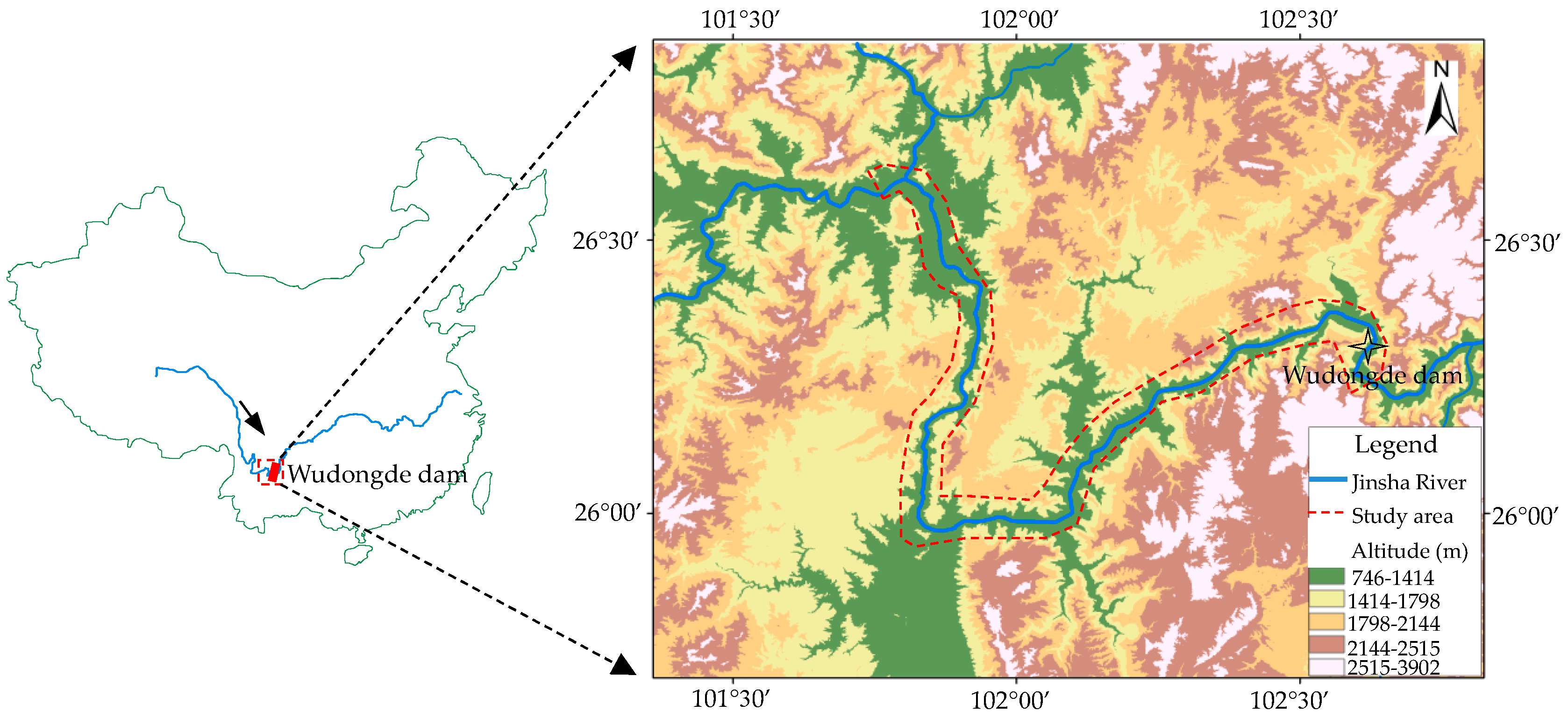
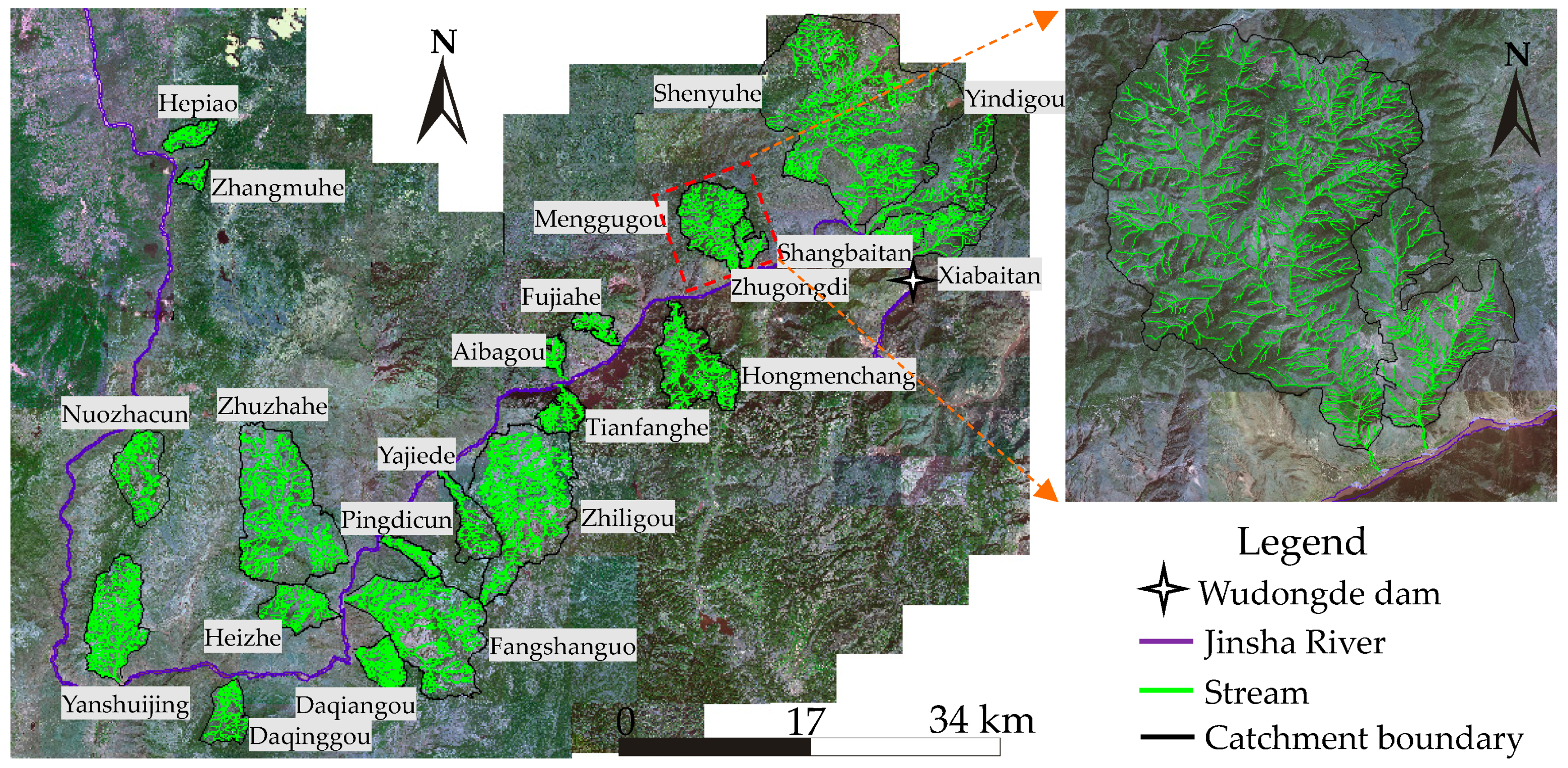
The study area (Figure 1) lies along the lower reaches of the Jinsha River and is the reservoir region of the Wudongde hydropower station, which is located in the mountains separating the Sichuan and Yunnan provinces. The Wudongde hydropower station is one of the four largest power plants in the lower reaches of the Jinsha River. The station controls a basin area of 406,100 km2, which occupies 86% of the Jinsha River. The studied section of Jinsha River is about 210 km long. The area of investigation along the Jinsha River was extended from the alluvial plain to the crest. Based on field investigations, 22 channelized debris flow gullies distributed on both sides of the Jinsha River were identified, as shown in Figure 2. Considering that loose materials from the debris flow gullies could enter the Jinsha River and affect the running of the power station, it is of great significance to carry out a susceptibility analysis for this area.
2.1. Geological and Tectonic Setting
The geology comprises two major components: a pre-Sinian crystalline basement and a Sinian-Cretaceous sedimentary cover. The former mainly consists of a series of metamorphic rocks (phyllite, slate and schist), which widely outcrops along the Jinsha River. The latter includes magmatic rocks (granite and quartz diorite) and sedimentary rocks (limestone, sandstone, mudstone and shale). Figure 3 shows the lithology along the Jinsha River. According to field investigations, three types of potential source materials for debris flows outcrop in the study area [31]: (1) the Longjie silt layer from the Late Pleistocene period, mainly composed of clayey silt, silt and sand; (2) the sediment of the Madianhe Group from the Holocene period, which is mainly composed of silt and gravel; (3) and the red-bed, Triassic and the Cretaceous argillaceous evaporites.
The study area is located in the eastern section of the Tethys-Himalaya tectonic domain, one of the tectonic zones of the Himalaya characterized by intense compressing and folding. The predominant structures are regional-scale faults constituting the famous Chuan-Dian N-S tectonic belt [32]. A total of 13 regional-scale faults that dominantly trend approximately N-S are situated in this region (Figure 4). Several strong earthquakes with magnitude greater than 6.0 have been triggered by these faults since 1955 [33], such as the Puduhe earthquake (Magnitude 6.3, 1985) triggered by the Puduhe fault, the Wozhangshan earthquake (Magnitude 6.5, 1995) triggered by the Tanglang-Yimeng fault, and the Panzhihua earthquake (Magnitude 6.1, 2008) triggered by the Mopanshan-Lvzhijiang fault. These earthquakes triggered a lot of rock falls and landslides and produced a large quantity of loose materials sufficient to potentially trigger debris flows in the drainages.
2.2. Geomorphological Setting
This area exhibits a mountain canyon geomorphology, with elevations ranging from 800 to 3600 m, as shown in Figure 1. Observed geomorphic features include cliffs, rocky slopes, ridges and Quaternary deposits along the river valleys. The average slope angles of the hillsides in the region vary from 30 to 45°. The slopes are rocky and poorly vegetated; the dominant species are grasses on the soils. The distributions of the river network and ridges are controlled by structures in some extent. The effect of high relief and structural control is also well reflected by deep gorges and narrow valleys carved by numerous streams.
2.3. Meteorological Setting
The study area experiences a low-latitude plateau subtropical monsoon meteorology, characterized by concentrated rainfall and distinct wet and dry seasons. The mean annual temperature is 20.9 °C, with the 32 year (from 1972 to 2003) mean annual precipitation being 1058 mm [34]. The rainy season concentrates from May to October, with a peak in July. The maximum 10-min, 1-h and 24-h rainfall rates recorded in 32 years are 21.7, 77.2 and 111.5 mm, respectively.
3. Influencing Parameters
The occurrence of debris flows is a complicated process that requires favorable terrain conditions, source conditions and hydrodynamic conditions [6,35]. This research selected the triggering area of the debris flow as the base spatial unit. Based on field investigations and previous studies in the study area [31,33,34], eight factors were selected as the environmental predictors for debris flows. They are lithology (P1), watershed area (P2), slope angle (P3), stream density (P4), length of the main stream (P5), curvature of the main stream (P6), distance from fault (P7), and vegetation cover ratio (P8). Note that rainfall is deemed as a triggering factor for debris flows in our study area. However, it was not considered in this work because it is relatively uniform throughout the area.
3.1. Lithology
The lithology is one of the main parameters influencing the occurrence of debris flows in the study area [31]. It controls the stability of slopes and thus affects the debris supply for drainages. Filed surveys suggest that Quaternary deposits are most prone to the initiation of debris flows, whereas magmatic rocks and limestones have the lowest susceptibility for the occurrence of debris flows.
3.2. Watershed Area
The watershed area is referenced to the rainfall that can be collected and to the volume of loose materials [7]. Debris flows in the study area primarily occurred in catchments with relatively larger areas, most probably because a larger watershed area could collect more rainfall and a larger volume of loose materials.
3.3. Slope Angle
3.4. Stream Density
The stream density is expressed as the total length of all the streams in a catchment divided by the total area [33,38]. This factor reflects the interactions among lithology, geological structures, and weathering degree of rocks in a catchment because drainages often develop in weak area [33]. In addition, it can affect the shape of a river’s hydrograph during a rainstorm [38]. Investigations suggest that catchments carved by numerous streams are prone to the initiation of debris flows.
3.5. Length of the Main Stream
The length of the main stream is also an important factor influencing the occurrence of debris flows in the study region. The longer the main stream is, the more deposits a debris flow could gather together and transport to the runout zone [7].
3.6. Curvature of the Main Stream
The curvature of the main stream is related to the ratio of the main stream’ curve length to its straight length [33]. It reflects the discharge capacity of debris flows. Field surveys indicate that a catchment with an abroad and straight channel often retains limited loose materials, which is not prone to the debris flow occurrence.
3.7. Distance from Fault
Faults play a crucial role in the initiation of debris flows in our study area. They trigger earthquakes, produce discontinuities in rocks, and as a consequence, furnish debris that can be mobilized. Field investigations suggest that catchments near faults are prone to experiencing debris flow events.
3.8. Vegetation Cover Ratio
The vegetation cover ratio is described as the ratio of the vegetation area to the watershed area [10]. The dominant species in the study area are grasses on the soils. The natural vegetation in the study area has been damaged because of irrational deforestation and reclamation, suggestive of the highly erosive capability of the flows, able to increase their volume as they move [31,34] A poor vegetation cover indicates a high chance for a catchment to suffer from rainfall and rock weathering, and therefore facilitates debris production.
The watershed area, slope angle, stream density, length of the main stream, curvature of the main stream, and distance from fault were derived from the digital elevation model (DEM) with a resolution of 2.5 m. The lithology was obtained from a 1:50,000 scale geological map. The vegetation cover ratio was derived from the SPOT5 remote sensing image. The environmental parameters were subdivided into classes (Table 1) based on previous studies in the study area [31,34]. A standardization method was adopted to rescale the data to a common numerical basis according to their influence on the debris flow occurrence, which was carried out by transforming raw data to scores [39]. The ratings of the influencing factors (Pi) are shown in Table 1.
4. Method
4.1. Rock Engineering System
The implementation of the rock engineering system (RES) method can be achieved through an interaction matrix, which is the basic analytical device used in RES for characterizing the influencing parameters and their interaction mechanisms relevant to a particular engineering problem [40,41]. In RES, all selected parameters associated with a problem are arranged along the leading diagonal of the interaction matrix. The influence of each parameter on any other parameter, which is called interaction, is placed in the corresponding off-diagonal cells. Traditionally, the off-diagonal cells are assigned numerical values to quantify the degree of the influence of one factor on the other factors, named “coding the matrix”. Various approaches have been proposed for coding the interaction matrix [42], such as the 0–1 binary, expert semi-quantitative (ESQ), and the continuous quantitative coding (CQC) methods. Among these methods, the ESQ coding is the most commonly used, whereby the interaction between the parameters is ranked based on a numerical scale. Typically, a scale from 0 to 4 is employed (Table 2) [28].
Figure 5 presents an example for the simplest interaction matrix with two factors. Note that the influence of i on j is often not the same as the influence of j on i, indicating that the interaction matrix is not symmetric. Generally, the interaction matrix can contain any number of variables, depending on the engineering objective and the level of analysis required [43]. Figure 6 shows the coding of a multiple-dimensional interaction matrix. A problem that contains N factors will have an interaction matrix of N rows by N columns. The column passing through Pi represents the influence of other parameters on Pi, while the row through Pi represents the influence of Pi on the remaining parameters. For example, the (i, j)-th element in the matrix represents the influence of parameter i on parameter j.
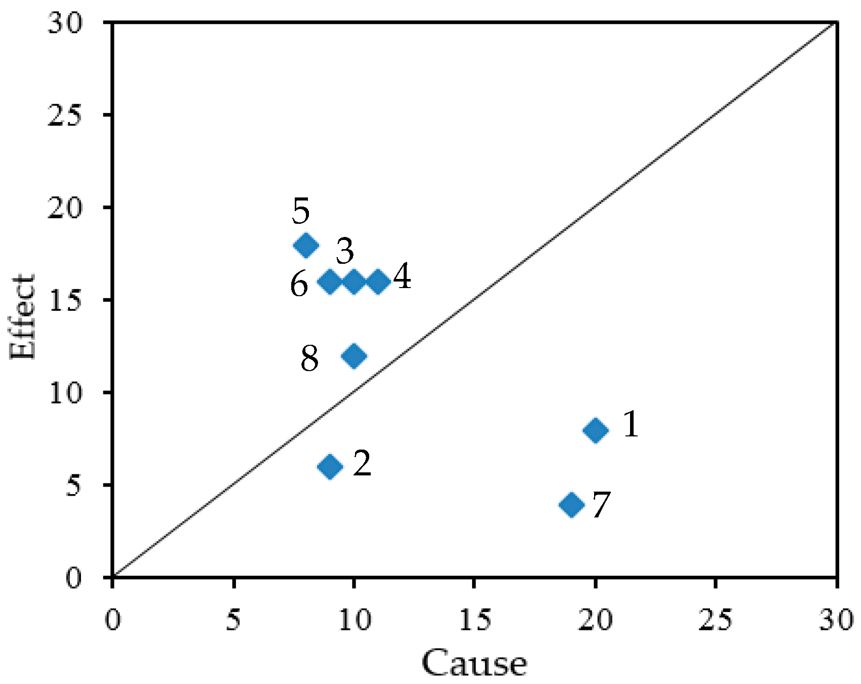
After coding the interaction matrix, the sum of each row and that of each column can be computed. For each parameter i, the sum of its row values and that of its column values are called the ‘‘cause’’ value (Ci) and the ‘‘effect’’ value (Ei), respectively. The coordinate values (Ci, Ei) for each parameter can be plotted in cause and effect space, forming the so-called cause–effect plot, which can help to understand the relative importance of each parameter within the system [43]. The percentage value of (C + E) can be used as the weighting of each parameter, which is given by:
4.2. Fuzzy C-Means Algorithm
Fuzzy C-means (FCM) clustering method proposed by Bezdek [29] is a well-known and powerful method in data mining and knowledge discovery. It generates a fuzzy partition based on the idea of partial membership expressed by the degree of membership of each object in a given cluster. In fuzzy clustering, each object has a degree of belonging to clusters rather than belonging completely to just one cluster [44].
Given a data set of N observations obtained from N regions, each represented by a vector of P attributes, Xj = (Xj1, Xj2, …, XjP), the algorithm is designed to partition the data set into C clusters (i.e., structural domains) by iteratively minimizing the fuzzy objective function which is expressed as follows [29]:
where uij represents the degree of membership of observation Xj in cluster i, m is the fuzziness index, which controls the fuzziness of the memberships, and d(Xj, Vi) is the distance between observation Xj and the ith cluster center Vi. m = 2 is deemed to be the best for most applications [29]. In this research, the value of P is 6 since there are six parameters that were used for structural domain determination.
5. Results and Discussion
5.1. RES Model for Debris Flow Susceptibility Assessment
With the selected eight parameters, an 8 by 8 interaction matrix was built according to Table 2, as shown in Table 3. For instance, considering that the lithology can be eroded and produce a different slope depending on its rheology, a value of 4 is assigned to the cell of the 1st row and 3th column in the matrix, suggesting that the lithology (P1) has a critical influence on the slope angle (P3). In addition, a value of 0 is assigned to the cell of the 3rd row and 1st column in the matrix, suggesting that lithology is not influenced by slope angles.
Based on the iteration matrix, the coordinates (Ci, Ei) of each parameter were calculated (Table 4). A cause–effect plot was drawn with the (Ci, Ei) coordinates, as shown in Figure 7. Each point in the plot represents a particular factor Pi. The cause–effect plot can help to distinguish between “less interactive” and “more interactive” parameters: the “more interactive” parameters are plotted in the upper left region, whereas the “less interactive” parameters are plotted in the lower right region [28]. Figure 7 indicates that P5 (length of the main stream) is more interactive than the other parameters, and it is greatly affected by the system. On the other hand, P1 (lithology) and P7 (distance from fault) have the maximum effect on the system.
The cause–effect plot also helps us to graphically compute the parameter interaction intensity and the parameter dominance. The interaction intensity of each parameter is represented by (C + E)/, and can be measured along the C = E line; the parameter dominance depends on the perpendicular distance from the parameter’s point representation to this line, which is calculated with (C − E)/ [28]. Figure 8 shows a histogram of the interaction intensity of each parameter. The histogram reveals that little changes in P2, P3, P4 and P5 will have great influence on the behavior of the system.
Table 4 lists the weightings of the influencing parameters computed by Equation (1), which follow the order of lithology > stream density > slope angle = length of the main stream > curvature of the main stream > distance from fault > vegetation cover ratio > watershed area.
5.2. Debris Flow Susceptibility Assessment
The RES model was applied to the 22 channelized debris flow gullies. The debris flow susceptibility index (SI) of each site was calculated by Equation (6), as listed in Table 5. In this work, the fuzzy C-means algorithm was adopted to divide the studied sites into three categories of debris flow susceptibility based on the RES model (RES_FCM). A debris flow susceptibility map was created, as shown in Figure 9. The classification results show that the susceptibility levels for nine of the debris flow gullies are high, nine are moderate and four are low, respectively.
5.3. Validation of the Model
The new model was validated by the field survey data. The actual conditions of the debris flow gullies were determined according to the principles listed in Table 6 based on the geological and environmental conditions, as shown in Table 5. The results show that among the 22 debris flow gullies, there are only two gullies (i.e., Yindigou and Zhangmuhe) that were assigned to different susceptibility groups compared with the actual conditions of the two gullies. The prediction accuracy of the new method is 90.9%, which is deemed satisfactory.
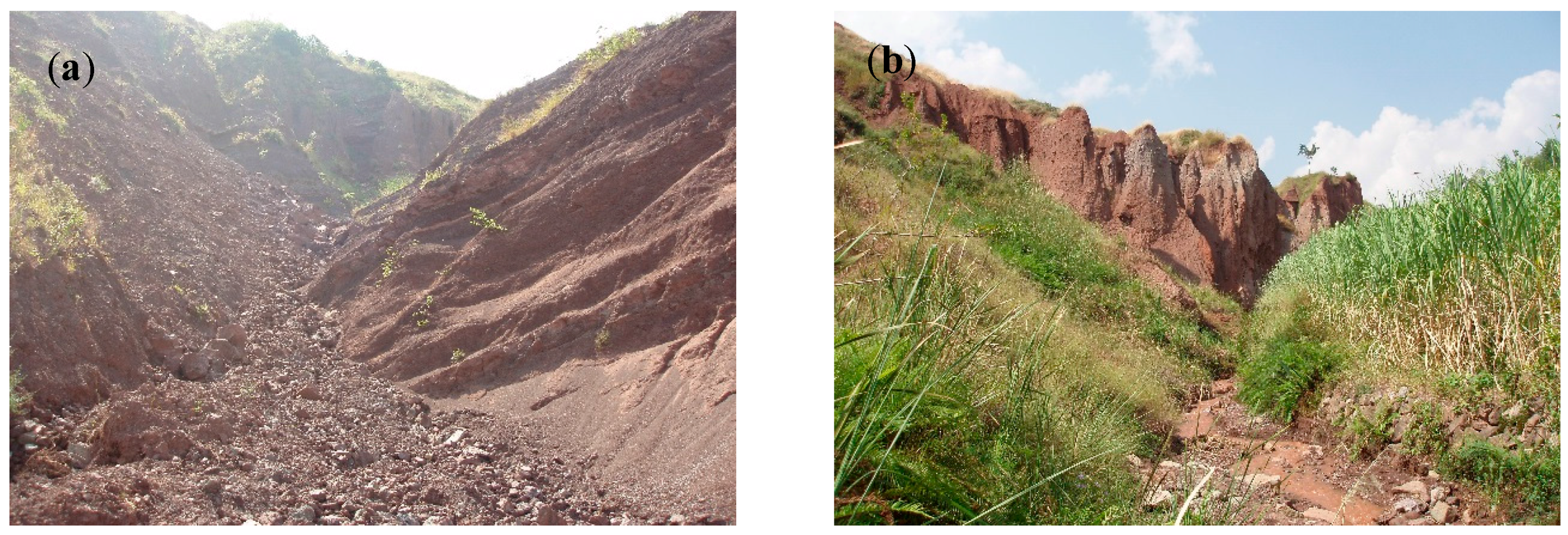
In this research, the RES based K-means algorithm (RES_KM) was used for comparison. The results show that the RES_FCM method and the RES_KM method provide very close evaluation results for most of the debris flow gullies. The difference between the results of the two methods lies in that the susceptibility level for the Shenyuhe debris flow gully was calculated to be moderate using the RES_FCM method, whereas the result obtained by the RES_KM method shows that the gully has low susceptibility level for debris flows. In fact, field investigation for the Shenyuhe debris flow gully shows that (1) a large amount of loose materials provided by landslides were deposited along the main channel (Figure 10a); (2) some slopes composed of sediments of the Madianhe Group are unstable; and (3) a small mudflow was observed to occur along a smooth-narrow gully (Figure 10b). Combined with the field investigations, it is more reasonable to partition the Shenyuhe gully into the moderate susceptibility group. According to Table 5, the prediction accuracy of the RES_KM method is 86.4%, which is smaller than that obtained by the RES_FCM method. In addition, the susceptibility levels for Yindigou and Zhangmuhe debris flow gullies obtained by the RES_FCM method are both higher than their actual conditions, indicating that the RES_FCM method does a slight overestimation of hazard; this goes towards security. However, the RES_KM method does a slight underestimation of hazard for the Shenyuhe debris flow gully; this does not go towards general safety. Therefore, the RES_FCM method performs better than the RES_KM method for assessing the susceptibility of debris flows.
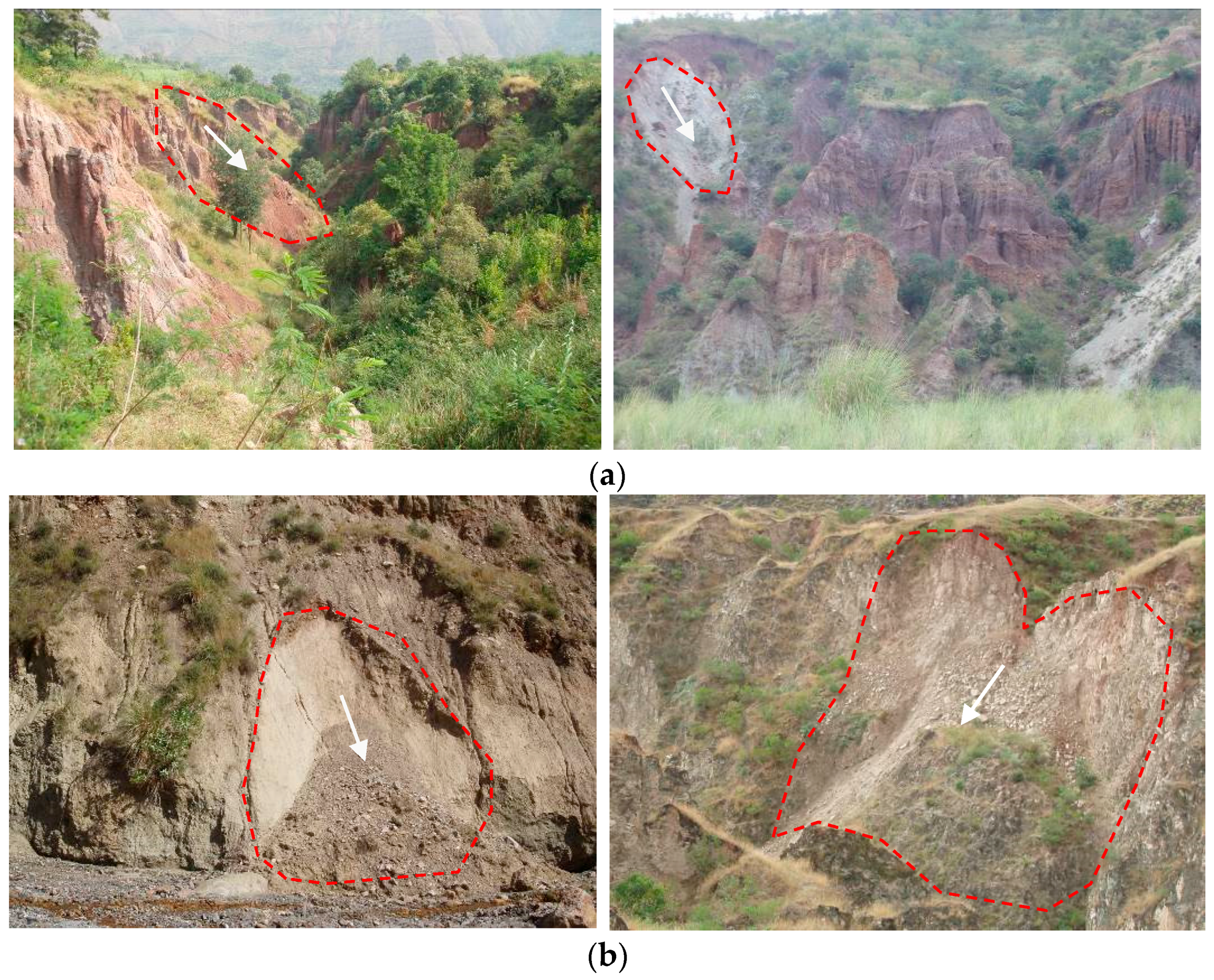
Figure 9 illustrates that the gullies categorized into high susceptibility zone are predominantly situated in the eastern part of the study area, signifying that this part is more prone to debris flows than anywhere else. In fact, field investigations suggest that the Quaternary deposits and the fine sand layer, which are not stable and prone to slope failures (Figure 11), are mainly distributed in the eastern part of the study area. Furthermore, the strong earthquakes triggered by faults have resulted in widespread landslides or rockfalls on these unstable rock formations. Failed slopes provide sufficient loose materials for drainages and hence facilitate the initiation of debris flows. Moreover, the distribution of high susceptibility zones is in accordance with the distribution of the regional faults (Figure 4). Therefore, the debris flow susceptibility map agrees well with the environmental features favorable for the initiation of debris flows in the study area.
6. Conclusions
This paper presents an application of the rock engineering system and fuzzy C-means algorithm (RES_FCM) for debris flow susceptibility assessment. A total of 22 channelized debris flow gullies located in the watershed of the Jinsha River close to the Wudongde dam site were investigated. The debris flow susceptibility of these gullies was assessed by introducing the concept of a susceptibility index (SI) based on the principles of RES. Eight parameters that are considered to be potential controls of debris flows were selected. The interactions among these parameters were determined using RES. The results show that the susceptibility levels for nine of the debris flow gullies are high, nine are moderate and four are low, respectively.
The RES based K-means algorithm (RES_KM) was used for comparison. The results show that the RES_FCM method and the RES_KM method provide very close evaluation results for most of the debris flow gullies, which are very similar to the evaluation results from the geological conditions in the study area. The new approach could be a simple but efficient tool for analyzing parameters influencing the occurrence of debris flows, and could be useful for evaluating the debris flow susceptibility.
This work only selected 22 large-scale debris flow gullies as our research object, considering that only large-scale debris flows could affect the stability of the dam; this could be helpful for debris flow hazard prevention. Further research work on the application of the proposed method to the total of the Wudongde dam area is necessary.
Acknowledgments
This work was financially supported by the National Natural Science Foundation of China (NSFC) (Nos. 41602327 and 41372324), and China Postdoctoral Science Foundation funded project (No. 2015M580135). The authors are grateful to two anonymous reviewers for their excellent reviews that helped to improve the manuscript.
Author Contributions
All authors were responsible for different parts of this paper. Yanyan Li, Jianping Chen conducted field investigations and wrote the whole paper; Yanjun Shang and Honggang Wang provided useful advice for data analysis and revised the paper.
Conflicts of Interest
The authors declare no conflict of interest.
References
- Rickenmann, D. Empirical relationships for debris flows. Nat. Hazards 1999, 19, 47–77. [Google Scholar] [CrossRef]
- Conway, S.J.; Decaulne, A.; Balme, M.R.; Murray, J.B.; Towner, M.C. A new approach to estimating hazard posed by debris flows in the Westfjords of Iceland. Geomorphology 2010, 114, 556–572. [Google Scholar] [CrossRef]
- Kanji, M.A.; Cruz, P.T.; Massad, F. Debris flow affecting the Cubatão oil refinery, Brazil. Landslides 2008, 5, 71–82. [Google Scholar] [CrossRef]
- Kappes, M.S.; Malet, J.P.; Remaître, A.; Horton, P.; Jaboyedoff, M.; Bell, R. Assessment of debris-flow susceptibility at medium-scale in the Barcelonnette Basin, France. Nat. Hazards Earth Syst. Sci. 2011, 11, 627–641. [Google Scholar] [CrossRef]
- Horton, P.; Jaboyedoff, M.; Rudaz, B.; Zimmermann, M. Flow-R, a model for susceptibility mapping of debris flows and other gravitational hazards at a regional scale. Nat. Hazards Earth Syst. Sci. 2013, 13, 869–885. [Google Scholar] [CrossRef] [Green Version]
- Chang, T.C.; Chien, Y.H. The application of genetic algorithm in debris flow prediction. Environ. Geol. 2007, 53, 339–347. [Google Scholar] [CrossRef]
- Chang, T.C.; Chao, R.J. Application of back-propagation networks in debris flow prediction. Eng. Geol. 2006, 85, 270–280. [Google Scholar] [CrossRef]
- Chang, T.C. Risk degree of debris flow applying neural networks. Nat. Hazards 2007, 42, 209–224. [Google Scholar] [CrossRef]
- Conforti, M.; Pascale, S.; Robustelli, G.; Sdao, F. Evaluation of prediction capability of the artificial neural networks for mapping landslide susceptibility in the Turbolo River catchment (northern Calabria, Italy). Catena 2014, 113, 236–250. [Google Scholar] [CrossRef]
- Liu, C.N.; Dong, J.J.; Peng, Y.F.; Huang, H.F. Effects of strong ground motion on the susceptibility of gully type debris flows. Eng. Geol. 2009, 104, 241–253. [Google Scholar] [CrossRef]
- Wan, S.; Lei, T.C. A knowledge-based decision support system to analyze the debris-flow problems at Chen-Yu-Lan River, Taiwan. Knowl.-Based Syst. 2009, 22, 580–588. [Google Scholar] [CrossRef]
- Dai, F.C.; Lee, C.F.; Tham, L.G.; Ng, K.C.; Shun, W.L. Logistic regression modelling of storm-induced shallow landsliding in time and space on natural terrain of Lantau Island, Hong Kong. Bull. Eng. Geol. Environ. 2004, 63, 315–327. [Google Scholar] [CrossRef]
- Ayalew, L.; Yamagishi, H. The application of GIS-based logistic regression for landslide susceptibility mapping in the Kakuda-Yahiko Mountains, central Japan. Geomorphology 2005, 65, 15–31. [Google Scholar] [CrossRef]
- Greco, R.; Sorriso-Valvo, M.; Catalano, E. Logistic regression analysis in the evaluation of mass movements susceptibility: The Aspromonte case study, Calabria, Italy. Eng. Geol. 2007, 89, 47–66. [Google Scholar] [CrossRef]
- Manzo, G.; Tofani, V.; Segoni, S.; Battistini, A.; Catani, F. GIS techniques for regional-scale landslide susceptibility assessment: The Sicily (Italy) case study. Int. J. Geogr. Inf. Sci. 2013, 27, 1433–1452. [Google Scholar] [CrossRef]
- Dong, J.J.; Lee, C.T.; Tung, Y.H.; Liu, C.N.; Lin, K.P.; Lee, J.F. The role of the sediment budget in understanding debris flow susceptibility. Earth Surf. Proc. Landf. 2009, 34, 1612–1624. [Google Scholar] [CrossRef]
- Bertrand, M.; Liébault, F.; Piégay, H. Debris-flow susceptibility of upland catchments. Nat. Hazards 2013, 67, 497–511. [Google Scholar] [CrossRef]
- Song, Y.Q.; Gong, J.H.; Gao, S.; Wang, D.C.; Cui, T.J.; Li, Y.; Wei, B.Q. Susceptibility assessment of earthquake-induced landslides using Bayesian network: A case study in Beichuan, China. Comput. Geosci. 2012, 42, 189–199. [Google Scholar] [CrossRef]
- Ahmed, B.; Dewan, A. Application of bivariate and multivariate statistical techniques in landslide susceptibility modeling in Chittagong city corporation, Bangladesh. Remote Sens. 2017, 42, 304. [Google Scholar] [CrossRef]
- Baeza, C.; Corominas, J. Assessment of shallow landslide susceptibility by means of multivariate statistical techniques. Earth Surf. Proc. Landf. 2001, 26, 1251–1263. [Google Scholar] [CrossRef]
- Guzzetti, F.; Reichenbach, P.; Ardizzone, F.; Cardinali, M.; Galli, M. Estimating the quality of landslide susceptibility models. Geomorphology 2006, 81, 166–184. [Google Scholar] [CrossRef]
- Xu, W.; Jing, S.; Yu, W.; Wang, Z.; Zhang, G.; Huang, J. A comparison between Bayes discriminant analysis and logistic regression for prediction of debris flow in southwest Sichuan, China. Geomorphology 2013, 201, 45–51. [Google Scholar] [CrossRef]
- Kayastha, P.; Dhital, M.R.; De Smedt, F. Application of the analytical hierarchy process (AHP) for landslide susceptibility mapping: A case study from the Tinau watershed, west Nepal. Comput. Geosci. 2013, 52, 398–408. [Google Scholar] [CrossRef]
- Meyer, N.K.; Schwanghart, W.; Korup, O.; Romstad, B.; Etzelmüller, B. Estimating the topographic predictability of debris flows. Geomorphology 2014, 207, 114–125. [Google Scholar] [CrossRef]
- Yalcin, A. GIS-based landslide susceptibility mapping using analytical hierarchy process and bivariate statistics in Ardesen (Turkey): Comparisons of results and confirmations. Catena 2008, 72, 1–12. [Google Scholar] [CrossRef]
- Yalcin, A.; Reis, S.; Aydinoglu, A.C.; Yomralioglu, T. A GIS-based comparative study of frequency ratio, analytical hierarchy process, bivariate statistics and logistics regression methods for landslide susceptibility mapping in Trabzon, NE Turkey. Catena 2011, 85, 274–287. [Google Scholar] [CrossRef]
- Pradhan, B. Landslide susceptibility mapping of a catchment area using frequency ratio, fuzzy logic and multivariate logistic regression approaches. J. Indian Soc. Remote 2010, 38, 301–320. [Google Scholar] [CrossRef]
- Hudson, J.A. Rock Engineering Systems: Theory and Practice; Ellis Horwood Ltd.: Chichester, UK, 1992; pp. 154–185. [Google Scholar]
- Bezdek, J.C. Pattern Recognition with Fuzzy Objective Function Algorithms; Plenum Press: New York, NY, USA, 1981; pp. 203–239. [Google Scholar]
- Li, Y.Y.; Chen, J.P.; Shang, Y.J. An RVM-based model for assessing the failure probability of slopes along the Jinsha River, close to the Wudongde dam site, China. Sustainability 2017, 9, 32. [Google Scholar] [CrossRef]
- Niu, C. Index Selection and Rating for Debris Flow Hazard Assessment. Ph.D. Thesis, Jilin University, Changchun, China, 2013; p. 143. [Google Scholar]
- Chen, H.; Hu, J.M.; Qu, H.J.; Wu, G.L. Early Mesozoic structural deformation in the Chuandian N-S Tectonic Belt, China. Sci. China Ser. D 2011, 54, 1651–1664. [Google Scholar] [CrossRef]
- Zhang, W.; Chen, J.P.; Wang, Q.; An, Y.; Qian, X.; Xiang, L.; He, L. Susceptibility analysis of large-scale debris flows based on combination weighting and extension methods. Nat. Hazards 2013, 66, 1073–1100. [Google Scholar] [CrossRef]
- Zhang, W.; Li, H.Z.; Chen, J.P.; Zhang, C.; Xu, L.M.; Sang, W.F. Comprehensive hazard assessment and protection of debris flows along Jinsha River close to the Wudongde dam site in China. Nat. Hazards 2011, 58, 459–477. [Google Scholar] [CrossRef]
- Hu, W.; Xu, Q.; Rui, C.; Huang, R.Q.; van Asch, T.W.J.; Zhu, X.; Xu, Q.Q. An instrumented flume to investigate the initiation mechanism of the post-earthquake huge debris flow in the southwest of China. Bull. Eng. Geol. Environ. 2015, 74, 393–404. [Google Scholar] [CrossRef]
- Lin, P.S.; Lin, J.Y.; Hung, J.C.; Yang, M.D. Assessing debris-flow hazard in a watershed in Taiwan. Eng. Geol. 2002, 66, 295–313. [Google Scholar] [CrossRef]
- Rickenmann, D.; Zimmermann, M. The 1987 debris flows in Switzerland: Documentation and analysis. Geomorphology 1993, 8, 175–189. [Google Scholar] [CrossRef]
- Lei, T.C.; Wan, S.; Chou, T.Y.; Pai, H.C. The knowledge expression on debris flow potential analysis through PCA + LDA and rough sets theory: A case study of Chen-Yu-Lan watershed, Nantou, Taiwan. Environ. Earth Sci. 2011, 63, 981–997. [Google Scholar] [CrossRef]
- Mousavi, S.M.; Omidvar, B.; Ghazban, F.; Feyzi, R. Quantitative risk analysis for earthquake-induced landslides—Emamzadeh Ali, Iran. Eng. Geol. 2011, 122, 191–203. [Google Scholar] [CrossRef]
- Hudson, J.A.; Harrison, J.P. A new approach to studying complete rock engineering problems. Q. J. Eng. Geol. Hydrogeol. 1992, 25, 93–105. [Google Scholar] [CrossRef]
- Huang, R.; Huang, J.; Ju, N.; Li, Y. Automated tunnel rock classification using rock engineering systems. Eng. Geol. 2013, 156, 20–27. [Google Scholar] [CrossRef]
- Faramarzi, F.; Mansouri, H.; Ebrahimi Farsangi, M.A. A rock engineering systems based model to predict rock fragmentation by blasting. Int. J. Rock Mech. Min. Sci. 2013, 60, 82–94. [Google Scholar] [CrossRef]
- Jiao, Y.; Hudson, J.A. The fully-coupled model for rock engineering systems. Int. J. Rock Mech. Min. Sci. 1995, 32, 491–512. [Google Scholar] [CrossRef]
- Zhang, B.; Qin, S.; Wang, W.; Wang, D.; Xue, L. Data stream clustering based on Fuzzy C-Mean algorithm and entropy theory. Signal Process. 2016, 126, 111–116. [Google Scholar] [CrossRef]
- Hammah, R.E.; Curran, J.H. Fuzzy cluster algorithm for the automatic identification of joint sets. Int. J. Rock Mech. Min. Sci. 1998, 35, 889–905. [Google Scholar] [CrossRef]
Figure 1.
Location map of the study area [30].
Figure 1.
Location map of the study area [30].

Figure 2.
Location of the debris flow gullies.

Figure 3.
Lithology in the study area [31].
Figure 3.
Lithology in the study area [31].
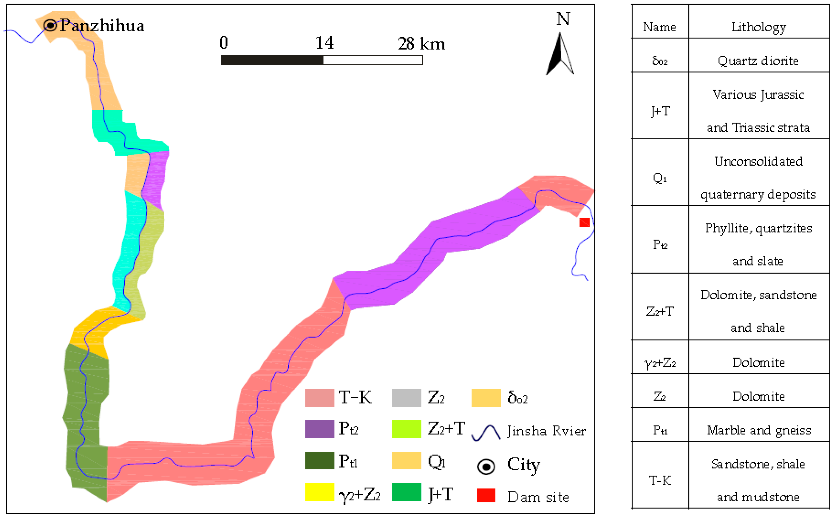
Figure 4.
Regional tectonic framework map [33].
Figure 4.
Regional tectonic framework map [33].
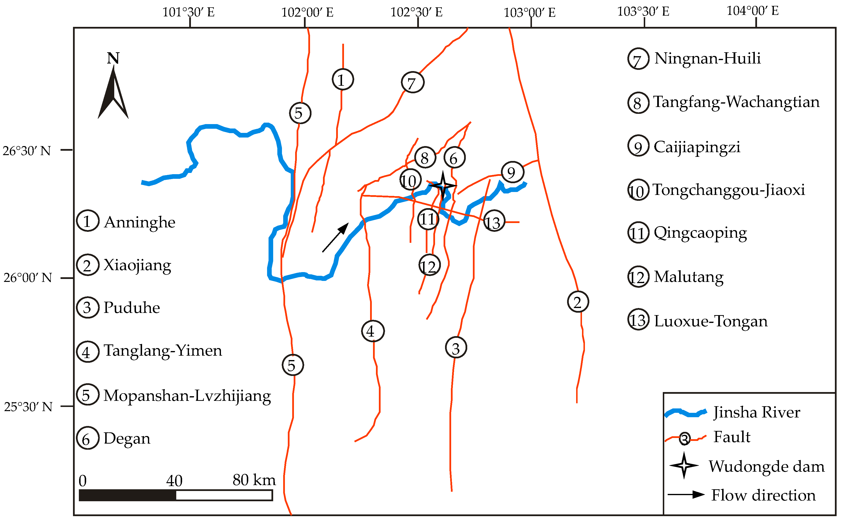
Figure 5.
General illustration of the interaction matrix with two factors [28].
Figure 5.
General illustration of the interaction matrix with two factors [28].
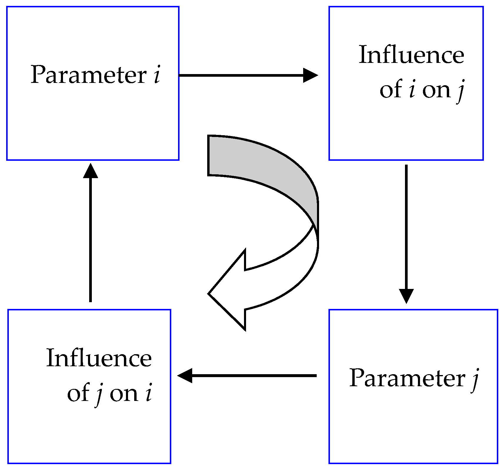
Figure 6.
Summation of coding values in the row and column through each parameter to establish the cause and effect coordinates [28].
Figure 6.
Summation of coding values in the row and column through each parameter to establish the cause and effect coordinates [28].
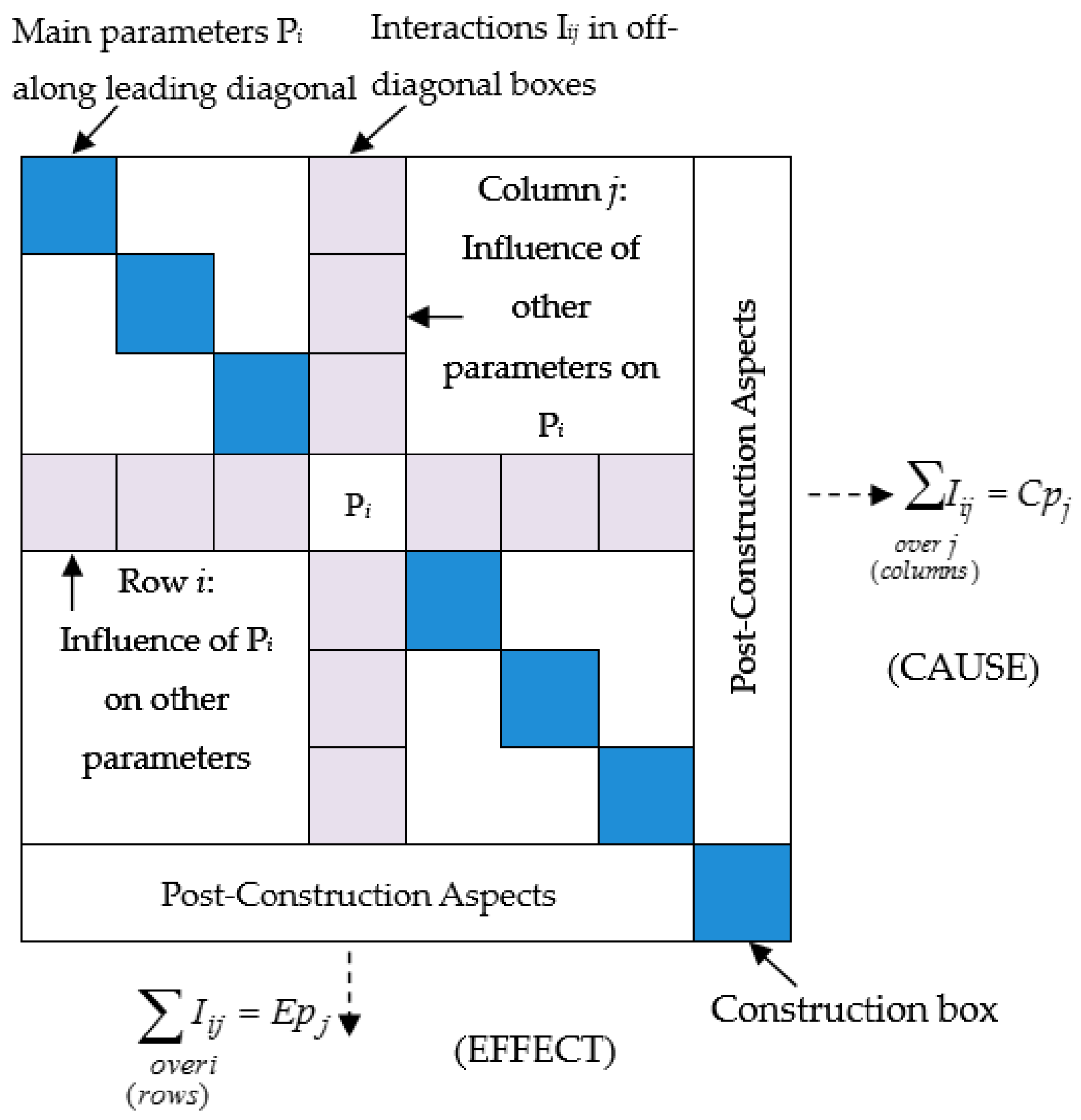
Figure 7.
Cause–effect diagram.

Figure 8.
Histogram of interactive intensity.
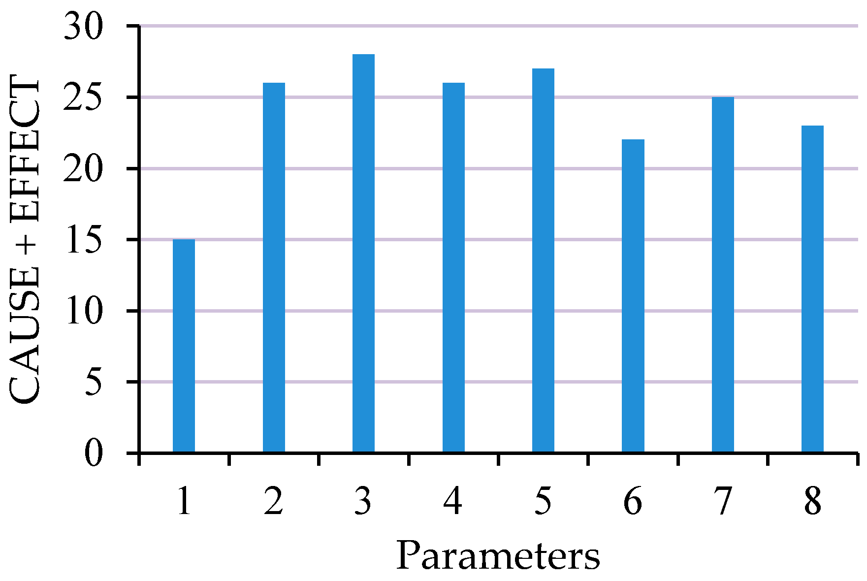
Figure 9.
Debris flow susceptibility map.
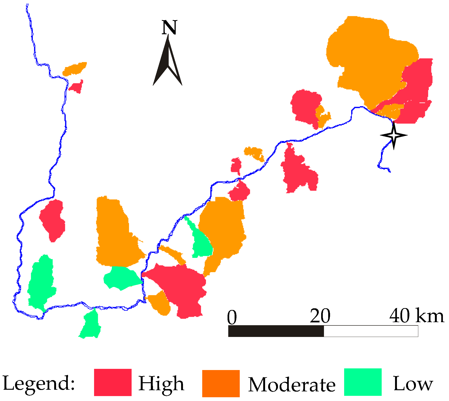
Figure 10.
Geological and environmental conditions of the Shenyuhe debris flow gully. (a) loose materials deposited along the main channel; (b) unstable slopes composed of sediments of the Madianhe Group and a small mudflow.
Figure 10.
Geological and environmental conditions of the Shenyuhe debris flow gully. (a) loose materials deposited along the main channel; (b) unstable slopes composed of sediments of the Madianhe Group and a small mudflow.

Figure 11.
Landslides occurred in the study area. (a) landslides on the Quaternary deposits; (b) landslides on the fine sand layer.
Figure 11.
Landslides occurred in the study area. (a) landslides on the Quaternary deposits; (b) landslides on the fine sand layer.


Table 1.
Classification of influencing factors and their rating values.
| Description | Rating | Description | Rating |
|---|---|---|---|
| 1. Lithology | 5. Length of the main stream (km) | ||
| Magmatic rocks, and limestones | 0 | <1 | 0 |
| Phyllite, slate and schist | 1 | 1–5 | 1 |
| Sandstones, mudstones, and shale | 2 | 5–10 | 2 |
| Quaternary deposits | 3 | >10 | 3 |
| 2. Watershed area (km2) | 6. Curvature of the main stream | ||
| <0.5 or >50 | 0 | <1.1 | 0 |
| 0.5–10 | 1 | 1.1–1.25 | 1 |
| 10–35 | 2 | 1.25–1.4 | 2 |
| 35–50 | 3 | >1.4 | 3 |
| 3. Slope angle (°) | 7. Distance from fault (km) | ||
| <15 | 0 | >0.6 | 0 |
| 15–25 | 1 | 0.4–0.6 | 1 |
| 25–32 | 2 | 0.2–0.4 | 2 |
| >32 | 3 | <0.2 | 3 |
| 4. Stream density (km/km2) | 8. Vegetation cover ratio | ||
| <5 | 0 | >0.75 | 0 |
| 5–10 | 1 | 0.5–0.75 | 1 |
| 10–20 | 2 | 0.25–0.5 | 2 |
| >20 | 3 | <0.25 | 3 |
Table 2.
ESQ interaction matrix coding [28].
Table 2.
ESQ interaction matrix coding [28].
| Coding | Description |
|---|---|
| 0 | No interaction |
| 1 | Weak interaction |
| 2 | Medium interaction |
| 3 | Strong interaction |
| 4 | Critical interaction |
Table 3.
Interaction matrix.
| P1 | 2 | 4 | 3 | 3 | 3 | 2 | 3 |
|---|---|---|---|---|---|---|---|
| 0 | P2 | 2 | 1 | 2 | 1 | 2 | 1 |
| 0 | 1 | P3 | 2 | 3 | 2 | 0 | 2 |
| 1 | 0 | 3 | P4 | 2 | 3 | 0 | 2 |
| 1 | 0 | 2 | 2 | P5 | 2 | 0 | 1 |
| 1 | 0 | 1 | 2 | 4 | P6 | 0 | 1 |
| 3 | 3 | 3 | 3 | 2 | 3 | P7 | 2 |
| 2 | 0 | 1 | 3 | 2 | 2 | 0 | P8 |
Table 4.
Coordinates and weightings of influencing parameters.
| Parameter | Ci | Ei | wi (%) |
|---|---|---|---|
| Lithology | 20 | 8 | 14.58 |
| Watershed area | 9 | 6 | 7.81 |
| Slope angle | 10 | 16 | 13.54 |
| Stream density | 11 | 16 | 14.06 |
| Length of the main stream | 8 | 18 | 13.54 |
| Curvature of the main stream | 9 | 16 | 13.02 |
| Distance from fault | 19 | 4 | 11.98 |
| Vegetation cover | 10 | 12 | 11.46 |
Table 5.
Susceptibility assessment results of the 22 debris flow gullies.
| Gullies | Influencing Parameters | SI | RES_KM | RES_FCM | Actual Condition | |||||||
|---|---|---|---|---|---|---|---|---|---|---|---|---|
| P1 | P2 | P3 | P4 | P5 | P6 | P7 | P8 | |||||
| Xiabaitan | T–K | 3.1 | 36.1 | 5.51 | 3.08 | 1.19 | 0 | 10 | 188.53 | High | High | High |
| Shangbaitan | T–K | 0.91 | 28.5 | 10.29 | 1.87 | 1.08 | 0 | 10 | 176.03 | Moderate | Moderate | Moderate |
| Menggugou | Pt2 | 37.1 | 41.37 | 6.73 | 10.52 | 1.13 | 0 | 40 | 205.19 | High | High | High |
| Aibagou | Pt2 | 6.66 | 42.13 | 8.43 | 5.09 | 1.19 | 0 | 20 | 187.49 | High | High | High |
| Nuozhacun | γ2 + Z2 | 32.61 | 40 | 4.96 | 10.5 | 1.17 | 0 | 10 | 194.78 | High | High | High |
| Zhugongdi | T–K | 6.5 | 41.8 | 6.24 | 4.98 | 1.15 | 0 | 15 | 176.55 | Moderate | Moderate | Moderate |
| Yindigou | T–K | 60.5 | 43.26 | 5.08 | 20.17 | 1.23 | 166 | 18 | 207.8 | High | High | Moderate |
| Fujiahe | Pt2 | 8.62 | 42.7 | 6.34 | 5.16 | 1.26 | 0 | 17 | 176.55 | Moderate | Moderate | Moderate |
| Zhangmuhe | Pt2 | 4.62 | 29.1 | 9.7 | 5.39 | 1.42 | 0 | 10 | 199.99 | High | High | Moderate |
| Hepiao | J + K | 9.1 | 29.6 | 9.9 | 6.83 | 1.32 | 0 | 30 | 175.51 | Moderate | Moderate | Moderate |
| Hongmenchang | Pt2 | 46.9 | 30 | 6.6 | 12.9 | 1.29 | 0 | 15 | 216.13 | High | High | High |
| Tianfanghe | Pt2 | 13.1 | 34 | 9.3 | 5.6 | 1.17 | 0 | 16 | 195.3 | High | High | High |
| Zhiligou | T–K | 120.6 | 24 | 6.3 | 15.8 | 1.28 | 0 | 25 | 181.76 | Moderate | Moderate | Moderate |
| Pingdicun | T–K | 24.2 | 17 | 5.9 | 9.9 | 1.14 | 3000 | 40 | 171.34 | Moderate | Moderate | Moderate |
| Fangshanguo | T–K | 98 | 28 | 4.63 | 20.2 | 1.38 | 6662 | 10 | 193.22 | High | High | High |
| Daqiangou | T–K | 18.9 | 29 | 10.95 | 5.1 | 1.11 | 18 | 17 | 174.46 | Moderate | Moderate | Moderate |
| Shenyuhe | T–K | 256 | 21 | 2.26 | 29.63 | 1.47 | 0 | 50 | 169.26 | Low | Moderate | Moderate |
| Zhuzhahe | T–K | 152.6 | 26.6 | 4.32 | 26.3 | 1.7 | 378 | 20 | 170.3 | Moderate | Moderate | Moderate |
| Heizhe | T–K | 51.7 | 13.5 | 5.12 | 13.9 | 1.15 | 3485 | 20 | 167.18 | Low | Low | Low |
| Yanshuijing | Pt1 | 48.58 | 22.6 | 9.25 | 14.43 | 1.22 | 0 | 5 | 153.63 | Low | Low | Low |
| Yajiede | T–K | 22.3 | 12 | 4.7 | 9.3 | 1.31 | 0 | 70 | 145.3 | Low | Low | Low |
| Daqinggou | T–K | 31.8 | 32 | 6.02 | 7.32 | 1.1 | 378 | 15 | 147.38 | Low | Low | Low |
Table 6.
Principles for assessing the actual condition of debris flow gullies.
| Level | Susceptibility Degree | Description |
|---|---|---|
| 1 | High | Abundance of loose materials accumulated on slopes, steep channels, inventory of debris flows |
| 2 | Moderate | Between levels 1 and 3 |
| 3 | Low | Absence of loose materials, smooth terrains , no debris flow record |
© 2017 by the authors. Licensee MDPI, Basel, Switzerland. This article is an open access article distributed under the terms and conditions of the Creative Commons Attribution (CC BY) license (http://creativecommons.org/licenses/by/4.0/).
Share and Cite
MDPI and ACS Style
Li, Y.; Wang, H.; Chen, J.; Shang, Y. Debris Flow Susceptibility Assessment in the Wudongde Dam Area, China Based on Rock Engineering System and Fuzzy C-Means Algorithm. Water 2017, 9, 669. https://doi.org/10.3390/w9090669
AMA Style
Li Y, Wang H, Chen J, Shang Y. Debris Flow Susceptibility Assessment in the Wudongde Dam Area, China Based on Rock Engineering System and Fuzzy C-Means Algorithm. Water. 2017; 9(9):669. https://doi.org/10.3390/w9090669
Chicago/Turabian StyleLi, Yanyan, Honggang Wang, Jianping Chen, and Yanjun Shang. 2017. "Debris Flow Susceptibility Assessment in the Wudongde Dam Area, China Based on Rock Engineering System and Fuzzy C-Means Algorithm" Water 9, no. 9: 669. https://doi.org/10.3390/w9090669
Note that from the first issue of 2016, this journal uses article numbers instead of page numbers. See further details here.