Analysis of Changes in Spatio-Temporal Patterns of Drought across South Korea


1
Department of Agricultural and Rural Engineering, Chungbuk National University, Cheongju 28644, Korea
2
K-Water Research Institute, Daejeon 34045, Korea
*
Author to whom correspondence should be addressed.
Water 2017, 9(9), 679; https://doi.org/10.3390/w9090679
Submission received: 26 July 2017
/
Revised: 4 September 2017
/
Accepted: 6 September 2017
/
Published: 7 September 2017
Abstract
:Since the climatic features of South Korea are highly complex and time variable, spatio-temporal-based drought frequency analysis is a prerequisite for drought risk management. The spatial extent of drought risk analysis in a bivariate framework has scarcely been applied in South Korea before. In this study, the spatio-temporal changes in drought events are investigated at 55 stations across South Korea during 1980–2015. A variety of probability distributions and copulas are applied, and the best fitted is selected on the basis the goodness of fit. The spatial distributions of primary and secondary return periods showed a high risk of drought due to the unusual precipitation pattern in the western coast areas and at Uljin station and a relative low risk of drought in the northwestern portion and surrounding areas of Yeongju, Uiseong, Boeun and Daejeon stations. Overall, the spatial distribution patterns of primary and secondary (Kendall) return periods are similar. However, their applicability changes according to the type of drought risk to be considered. The spatio-temporal quantification of the return period can be used for establishing the proper water demand and supply system and helps to overcome the challenges faced in the hydrometeorological regulations of reservoirs in the southwest coast.
1. Introduction
Drought is a natural phenomenon in which the natural water availability for a region is unusually low over an extended period, and the whole precipitation cycle is affected. According to studies based on changes in rainfall patterns in South Korea, an abrupt increase in greenhouse gases is the major cause of heavy rain, severe drought and heavy snow in some regions [1,2]. The Palmer Drought Severity Index (PDSI) was calculated using the climate change scenario based on the regional climate change model for the period of 1971–2100 [3]. It was concluded that the drought risk is likely to increase in South Korea despite an increase in general precipitation during the 21st century. The Standardized Precipitation Index (SPI) and PDSI were also studied together to reflect the seasonal trends of drought across South Korea [4].
In probability methods, the complex phenomena of drought should not be identified by only one characteristic of drought. The stochastic nature of droughts should be expressed using different drought variables. Drought identification and characterization are primary requirements for drought frequency analysis. There are various indices that have been used to measure the drought characteristics, and their use depends on the type of results needed. Drought indices were also derived from other hydrological and ecological variables [5,6,7]. Drought indices based on different climatic and hydrological variables may depict different regional and temporal patterns [8]. These indices are mostly based on a deficit in precipitation or discharge [9] to identify the drought. The precipitation deficit-based drought indices are more reliable and effective because they can directly reflect the deficit in rainfall based on a predetermined threshold. Secondly, despite orographic and land friction effects, precipitation is likely to perform more homogeneously than streamflow data. In addition, precipitation has often been recorded for a longer time period and tends to be less affected by human activities than streamflow data. Therefore, in this study, a drought event is defined using the truncation level approach applicable to precipitation time series and of direct relevance to the water industry and to the environmental demands of the river system. The truncation level approach defines droughts as periods during which the rainfall is below a certain truncation level [10].
Due to the complex nature of meteorological drought events, one drought variable is unable to provide a comprehensive evaluation. A bivariate distribution should be derived to express the correlated drought variables. In the case of flood studies, bivariate normal distributions [11], bivariate exponential distributions [12] and bivariate gamma distributions [13] or rainfall-runoff hydrological models [14,15] are often applied. The major drawbacks of these bivariate distributions are that the individual behavior of random variables must be characterized by the same parametric family of univariate distributions [16]. In the case of drought studies, the joint distributions are analytically acquired, by either assuming drought characteristics to be independent identically random variables [17] or assuming that they belong to the same marginal distribution function and have explicit bivariate forms (e.g., bivariate normal, bivariate exponential, bivariate gamma) [18]. However, the two above stated assumptions are not satisfied in most of the cases, because the drought variables (drought duration and severity) are highly correlated and may belong to different marginal distributions. Copula theory provides the solution of the above stated problems. The copula can preserve the dependence structure and different distribution characteristics of the drought variables. In addition, joint distributions of drought duration and severity can be derived using the nonparametric kernel estimator method [19] and the entropy-based method [20].
Copula theory, introduced by [21], has been used to join univariate distribution functions to form multivariate distribution functions based on the dependence structure among random variables. Therefore, during the last decade, copulas have emerged as a new multivariate modeling method in hydrology [22]. The commonly-used copulas in hydrology belong to two types: elliptical type (normal and Student t) and the Archimedean type (Clayton, Gumbel, Joe, Frank and Ali-Mikhail-Haq) [22,23]. For fitting of a copula, several marginal distributions have been used to fit drought duration and severity. Those marginal distributions include exponential (exp), gamma (gam), generalized extreme value (gev), generalized logistic (glo), generalized normal (gno), general Pareto (gpa), Gumbel (gum), lognormal (ln3), Pearson Type 3 (pe3) and Weibull (wei). The parameters of copulas are usually estimated using the maximum pseudo-likelihood or the inversion of Kendall’s method [23]. To select the appropriate marginal distribution of copulas, the goodness of fit is usually applied using the least root mean square error (RMSE), the Kolmogorov–Smirnov (KS) test, the Anderson–Darling (AD) test, the Akaike information criterion (AIC), ordinary least squares (OLS) and the Bayesian information criterion (BIC) [24].
2. Materials and Methods
The precipitation in South Korea has a high spatial and time variability [25]. Furthermore, most of the precipitation in South Korea falls during the summer season; this is because of the coincident typhoon season in the western North Pacific. Due to the complex topographical and climatic features of South Korea, the absence of the ability to recognize spatial characteristics is one of the main obstacles of drought analysis. Since the effect of drought is slowly moving to adjacent areas and thus spatio-temporal analysis of drought is gaining more importance among engineers and hydrologists for the design, planning and management of the water resource structure, it is necessary to investigate the spatial and temporal characterization of drought across South Korea. In this paper, drought risk analysis using ten commonly-used univariate probability distributions and six copulas (elliptical and Archimedean) was employed to analyze the spatial and temporal changing properties of drought. In addition, the top twenty historical drought events were selected for temporal analysis and for analyzing the changes in different bivariate return periods.
2.1. Study Area and Data
The Korean Meteorological Administration (KMA) manages climatological data at over 70 rainfall stations throughout South Korea. This study collected monthly precipitation data over 55 stations for more than 35 years (1980–2015). Only 55 rainfall stations were selected because of non-availability or missing precipitation data at a few rainfall stations. The Standardized Precipitation Index (SPI) proposed by [26] was used in this study for identifying the duration of drought events and to evaluate their severity. SPI was computed on the basis of fitting long-term rainfall data to the gamma distribution on any desired time scale, namely, 3 months, 6 months, 12 months and 24 months. The parameters of the gamma distribution are computed through the maximum likelihood estimation method. This fitted gamma distribution was then transformed to a standard normal distribution with the mean of zero and standard deviation of one [26]. The advantage of the SPI approach is that it allows a reliable and relatively easy comparison of precipitation deficit in the desired period between different locations and climates. This is because, in SPI, the rainfall is already normalized and compares the current rainfall with the average. In this study, the SPI time scale was chosen as 6 months, just as the time scales of dry and wet alterations in South Korea.
The characteristics of drought were extracted using the theory of run [10]. The theory of run method was proposed to identify drought duration and severity on the basis of the values that are below the selected truncation level. Therefore, run theory suggested a way to calculate the drought variables (drought duration and drought severity). The detailed description of the theory of run is provided by [10,27]. The duration of any drought was defined as the period of rainfall deficit, i.e., the cumulative time of negative values preceded and followed by positive values. The severity of any drought period starting at the -th month was defined as; . In other words, cumulated SPIs during the drought duration, defined by [26], are used to measure the magnitude of drought event and called the drought severity. In this study, −0.99 was selected as the truncation level in the run analysis. Therefore, the drought duration is the period when the SPI value was below −0.99, and the drought severity is the cumulative deficit during that drought event.
2.2. Marginal Distributions and Copulas
Copula distributions and cumulative distribution functions (CDFs) of probability distributions are shown in Table 1 and Table 2, respectively. In this study, the L-moment method is used to estimate the parameters of these marginal CDFs for drought duration and severity. Candidate probability distributions considered for this study are exponential (exp, 2 parameters), gamma (gam, 2 parameters), generalized extreme value (gev, 3 parameters), generalized logistic (glo, 3 parameters), generalized normal (gno, 3 parameters), general Pareto (gpa, 3 parameters), Gumbel (gum, 2 parameters), lognormal (ln3, 3 parameters), Pearson Type 3 (pe3, 3 parameters) and Weibull (wei, 3 parameters).
The root mean square error (RMSE) and Kolmogorov–Smirnov (KS) test [28] were used to choose the best fitted marginal distribution.
Let X = (X1, X2,..., Xn) be an n-dimensional random vector with a continuous marginal distribution function (CDF) F1, F2,…, Fn. [16] has the relationship between CDF H of X explained as follows:
where unique function is called the copula. The construction of a multivariate joint distribution model for H is accomplished in two parts: computation of the marginal CDF (F1, F2,…, Fn) and computation of the copula model (C).
In this study, the parameters of copulas were estimated using the maximum pseudo-likelihood [23] method. Candidate copula families used for the analysis were the elliptical and Archimedean copulas. Elliptical copulas include normal (Gaussian) and Student’s t, and Archimedean copulas include Clayton, Gumbel, Joe and Frank (Table 1). The parametric bootstrap-based Cramér–von Mises test (Sn) [29] and Akaike information criterion (AIC) [30] were used to assess the goodness of fit of all copulas. Bivariate joint distributions are estimated using the Copula package in R programming.
2.3. Return Period in a Bivariate Framework
Estimation of the return period has special importance in the planning and management of water resources. Let D denote the drought duration and S denote drought severity, then the return period in univariate settings can be defined as [31,32]:
and indicate the return period of the drought duration and severity, respectively. and indicate the cumulative distribution functions of drought duration and drought severity, respectively. For annual streamflow series, . Here, can be calculated using the theory of run and the Markov theorem [33].
where and . The unit of is months. According to [18], there are two cases of the bivariate return period: (i) D ≥ d and S ≥ s (drought variables exceeding another specific value); (ii) D ≥ d or S ≥ s (one of the drought variable exceeding another specific value).
where indicates the copula-based joint distribution function of the drought characteristics. ∧ denotes “and”, and ∨ denotes “or”.
2.4. Kendall Return Period
The standard definition of the return period may lead to under- or over-estimation of the correct values, and another definition of the bivariate return period was introduced by [31]. The Kendall return period is the average time between the occurrences of two supercritical drought events [34,35]. The Kendall return period is also known as the secondary return period. The primary return period, the one usually adopted in the applications for the designing of drought, may only provide partial and vague information about the realization of the events of interest. In fact, it only predicts that a critical event is expected to appear once in a given time interval (i.e., an average forecast). However, it would be more important to be able to calculate (1) the probability that a supercritical (destructive) event will show up at any given realization of the process (e.g., for any storm) and (2) how long will it take, on average, for a supercritical event to appear. As a fundamental result, both questions can now easily be answered using Kendall’s return period: the first one by defined below and the second one by considering the secondary return period given by Equation (7). The secondary return period provided a precise indication for performing risk analysis and may also yield useful hints for doing numerical simulations [36]. In addition to this, the use of and the secondary return period is more the appropriate approach to problems of (multivariate) risk assessment. In this study, we also adopted the secondary return period for the evaluation of drought risk within South Korea and compared with the joint return periods computed based on the routine computation procedure. To calculate Kendall’s return period, the occurrence probability should be computed first. Kendall’s distribution can be defined as . The related secondary return period was obtained via:
indicates the critical probability level, and denotes the Kendall distribution function. The for copulas of Archimedean family is as follows:
where denotes the right derivative of the generating function . For instance, this function for the Gumbel–Hougaard copula can be defined as;
The critical probability levels (t) were computed as follows:
Understanding Kendall’s return periods from a practical point of view is easier. Suppose is the critical return period specified via the design requirements. In the case of water resource management, the engineers are always interested in designing a water-supply system that can deliver a suitable amount of water under a specified extreme drought event that (on average) occurs once every years. Then, by inverting Equation (7), a critical probability level can be computed, and subcritical, non-threatening events can also be identified.
The Kendall distribution function related to the Clayton copula can be expressed as follows:
Similarly, the value of can be extended to Frank copulas:
The detailed description of the function for other copula families can be found in [23]. The coherent notation of the multivariate threshold and the total order in multidimensional Euclidean spaces was introduced by [31], used for the calculation of the secondary return period. They introduced notation for the multivariate quantile and purposed different methods to identify critical design events in the presence of several dependent variables.
3. Results
3.1. Drought Characteristics across South Korea during 1980–2015
Based on the SPI truncation level approach, different drought characteristics were extracted at 55 rainfall stations (Table 3). These characteristics include total number of drought events, mean drought duration, mean drought severity and drought event of longest duration at each rainfall station. The most severe drought lasted for 13 months at Jecheon rainfall station with the average drought duration and severity values of 3.43 months and 5.14, respectively. However, the total number of recorded drought events at Jecheon is 23 (relatively low). The maximum of 33 drought events was recorded at Tongyeong rainfall station. However, the average duration and severity values at Tongyeong are relatively low (1.97, 2.78, respectively), because most of the drought events have a duration of one or two months.
The regional frequency analysis using the L-moment method is suitable for stationary data. Therefore, identifying the trends and significance of non-stationarity is important in drought frequency analysis. In this study, the Mann–Kendall (M-K) nonparametric trend detection method was used to analyze the trends in drought series on the basis of SPI values. The significance of the trends was evaluated using the 95% confidence interval. The M-K trend test results showed that most of the stations are characterized by non-significant changes in drought duration and severity. Therefore, the null hypothesis was accepted, and the p-value showed that there was no evidence to reject the null hypothesis (there is no trend). Overall, the distributions of changes in drought duration and drought severity are spatially consistent across South Korea.
Based on SPI analysis, it was noticed that most of the short duration drought events lie between October and April. This is because of synoptic disturbances, typhoons or convective systems within the air mass, causing heavy rainfall during the summer season and low rainfall during the winter season.
3.2. Marginal Probability Distributions of Drought Duration and Severity
The first step to perform the bivariate frequency analysis of drought duration and severity is to choose the best fitted marginal distribution function for each rainfall station. To accomplish this task, ten candidate distributions as mentioned in Section 2.2, were considered for RMSE and the KS-test statistics. All of the distributions pass the KS test at the 99% (α = 0.01) significant level. The smaller the value of p in the KS-test, the stronger the evidence we have against the null hypothesis.
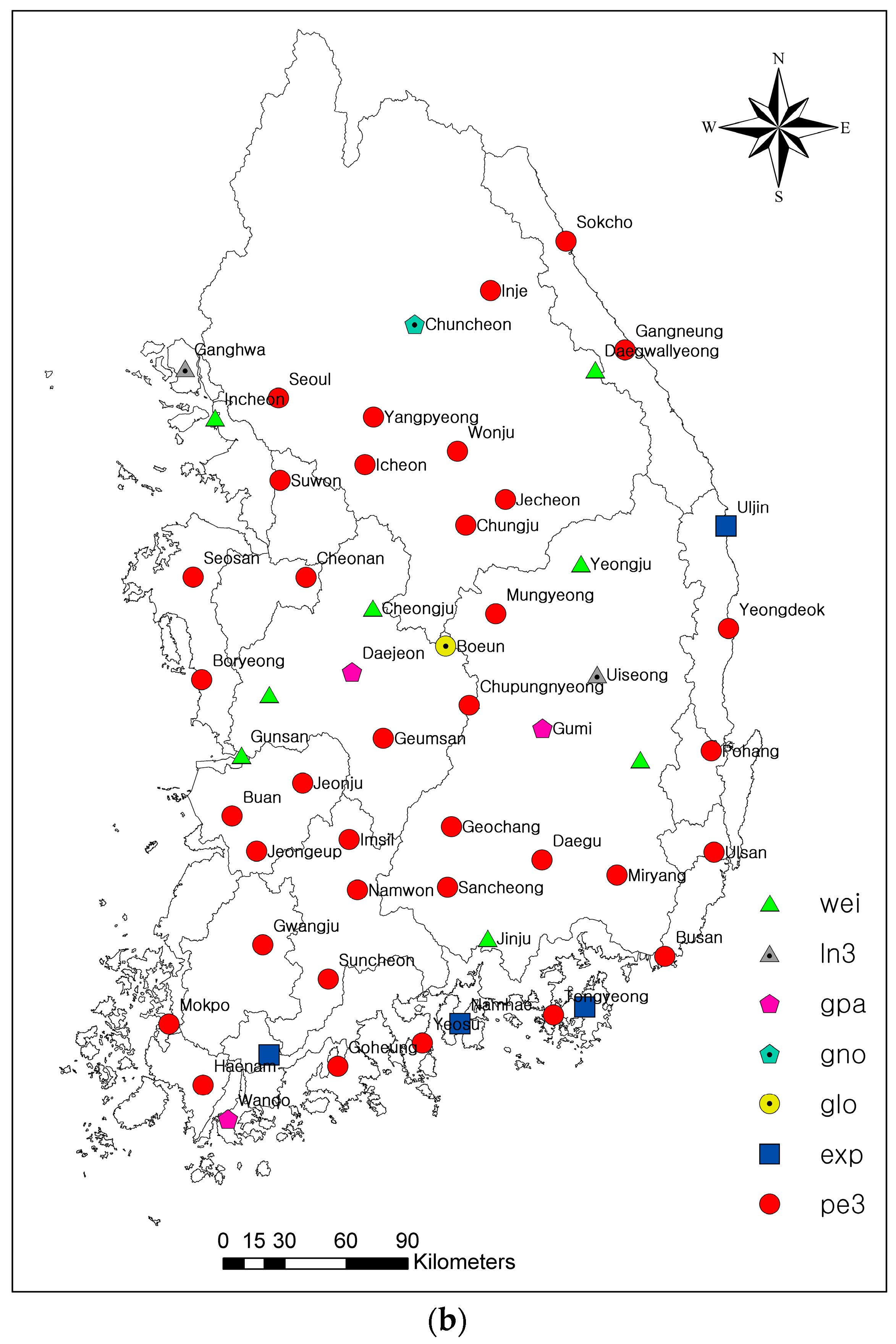
The results of the goodness of fit test and estimated parameters are shown only for the Jecheon rainfall station in Table 4. The top four best fitted marginal distributions of both drought duration and severity are marked with bold font in Table 4. In the case of duration, the top four best fitted marginal distributions are pe3, exp, gam and wei. In the case of severity, the top four best fitted marginal distributions are gam, gpa, pe3 and wei. Moreover, the visual comparison between empirical and theoretical cumulative distribution functions (CDFs) for the top four best fitted distributions of duration and severity are presented in Figure 1a,b, respectively. The estimated theoretical and empirical cumulative probabilities are quite close to each other, which indicates that these probability distributions perform fairly well. The final selected marginal distributions of drought duration and severity based on RMSE and the KS test for 55 rainfall stations are presented in Figure 2a,b. In the case of duration, most of the rainfall stations showed good agreement for four marginal distributions (exp, wei, gpa and pe3). However, in the case of severity, the selected marginal distributions are diverse (wei, ln3, gpa, gno, glo, exp and pe3). pe3 is the most common marginal distribution in the case of both drought duration and severity.
3.3. Application of Bivariate Copulas
The maximum pseudo-likelihood method was used to estimate the parameters of the candidate bivariate copulas. As an example, the results of the goodness of fit test and estimated parameters at Jecheon rainfall station are shown in Table 5. It is important to examine the dependence structure between the drought duration and severity. Besides, dependence measures are needed to procure a quantitative value of the dependence relation between drought variables.
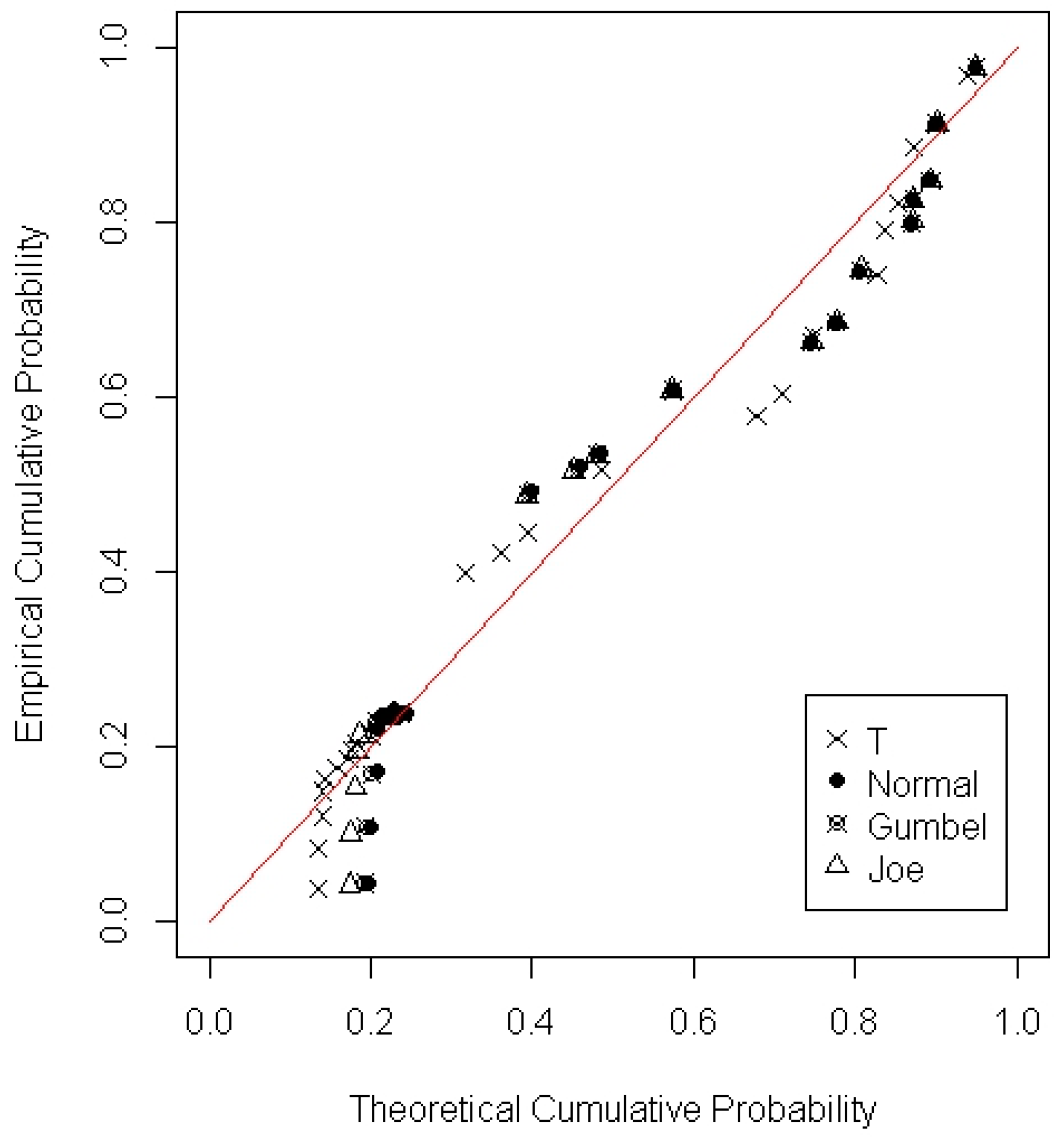
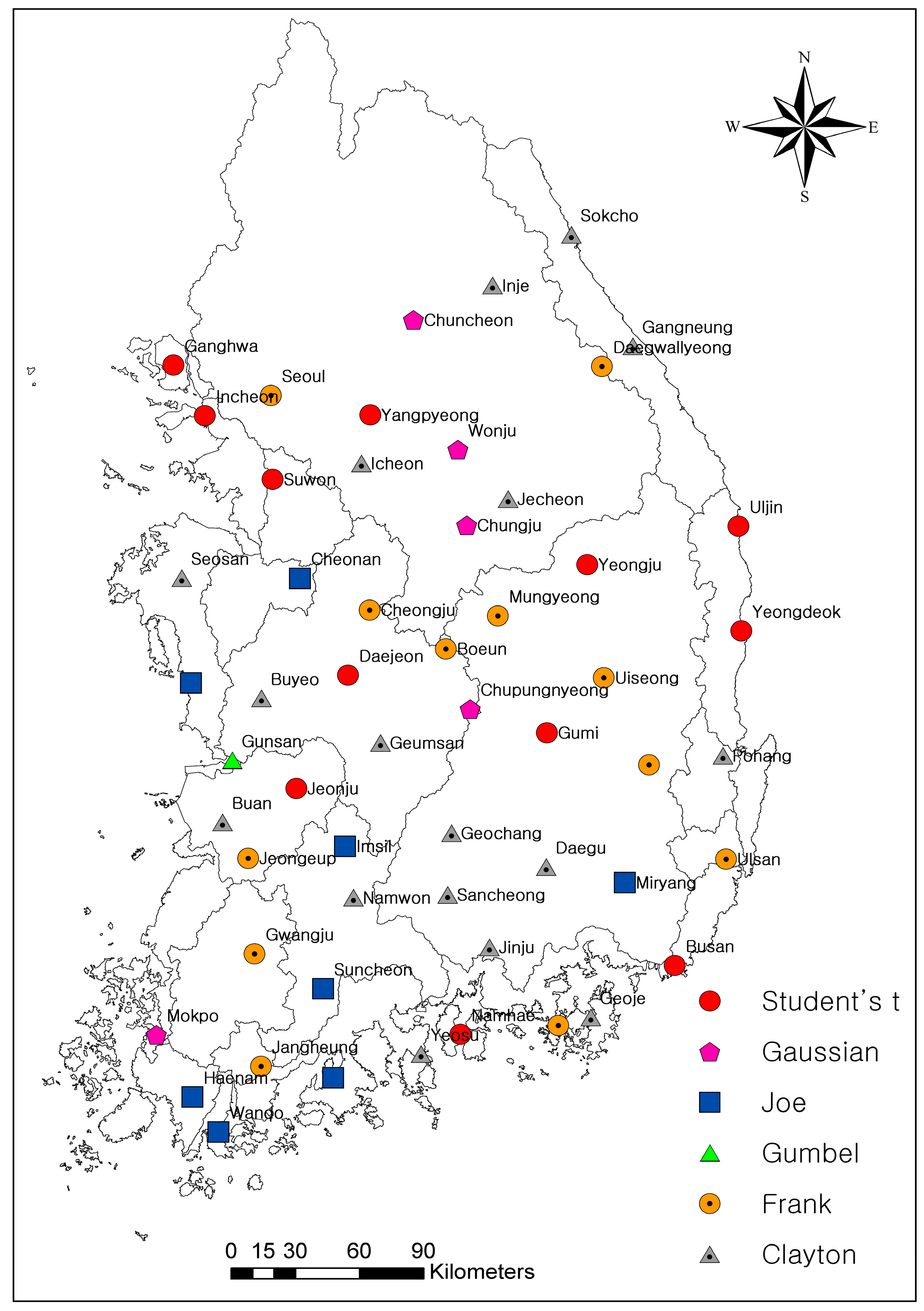
To accomplish this task, Pearson’s correlation measure of dependence is used, and its associated p-values were estimated using the criterion that the independence between variables is rejected when the p-value is less than 0.05. Further details about the p-value are provided in [37]. The Pearson’s correlation between drought duration and severity for 55 rainfall stations is shown in Table 6. Results indicate that there is a significant positive dependence between drought variables for all rainfall stations. After the evaluation of dependence between drought variables and fitting of different marginal distributions, copula functions were employed to model the joint distribution. The six candidate bivariate copulas mentioned in Section 2.2 were passed through the process of the goodness of fit using Sn and AIC statistics, for all rainfall stations. In this study, Sn statistics were tested at a significance level of 99% (α = 0.01). The top four best fitted copulas (normal, Student’s t, Gumbel and Joe) are marked with bold font. Moreover, the top four best fitted copulas were also evaluated by using the visual comparison between empirical and theoretical cumulative probabilities shown in Figure 3. The probability-probability (PP) plot indicates that the estimated cumulative probabilities agree well with the empirical ones. The final selected bivariate copulas of drought duration and severity based on the Sn and AIC statistics for 55 rainfall stations were presented in Figure 4. The goodness of fit indicates that the selection of bivariate copulas across South Korea is diverse.
3.4. Spatial Distribution of the Bivariate Return Period
The longer duration drought events are more concerned in frequency analysis because the effects of longer duration droughts are worse and have a high risk for water resource management. Therefore, only long enough drought duration and (or) large enough drought severity was selected for spatial frequency analysis of drought. In this study, long enough drought duration was six months, and large enough drought severity defined by SPI was 6.5. The spatial distribution of the “and” () return period was computed according to Equation (5) and then interpolated using the inverse distance weighted (IDW) technique, shown in Figure 5.
The average “and” return period characterized by a drought duration of six months and a drought severity of 6.5 was approximately 35.28 years over South Korea. Meanwhile, the minimum and maximum of the return period was 13.65 years at Goheung station and 56.90 years at Ganghwa station. It can be observed from Figure 5 that the northwestern portion and surrounding areas of Yeongju, Uiseong, Boeun and Daejeon have a relatively low risk of drought. This is because most of the drought events that occurred at Yeongju, Uiseong, Boeun and Daejeon stations had a duration closer to six months (long enough duration criterion) and drought severities closer to 6.5 (large enough severity criterion). Besides, the overall number of recorded drought events at the four stations is also relatively less. However, the southwestern coast and surrounding areas of Uljin have a high risk of drought. This is because the southwest coastal areas around Mokpo (Jangheung and Goheung) have extremely unusual rainfall patterns. For example, there was a record-breaking rainfall event (548 mm) that occurred due to the influence of Typhoon Agnes during 30 August–4 September 1981. On the other side, it can be noticed from Table 3 that the average duration and severity values of Jangheung were 3.35 and 5.03 and of Goheung were 3.29 and 5.12, respectively. Average drought duration and severity values indicate that among 55 stations, Jangheung and Goheung faced the second and third longest droughts after Jecheon (Table 3). In addition, the mid-latitude inland of South Korea (around Daejeon) is a high return period area affected by less severe droughts.
The spatial distribution of the “or” () return period was computed according to Equation (6) shown in Figure 6. The average “or” return period was characterized by a drought duration of six months and a drought severity of 6.5 was approximately 18.06 years, which is relatively lower than the “and” return period. Meanwhile, the minimum and maximum of the return period were 8.71 years at Jangheung station and 27.40 years at Yeongju station. Overall, the spatial patterns of the “and” (D ≥ d ∧ S ≥ s) return period in Figure 5 and the “or” (D ≥ d ∨ S ≥ s) return period in Figure 6 were the same, with the “and” return period showing higher severities and longer durations as compared to the “or” return period. This indicates that higher risk of droughts of longer durations mostly corresponded to the higher risk of droughts with a severe drought severity, which poses an increasing challenge for drought risk management and water resources management.
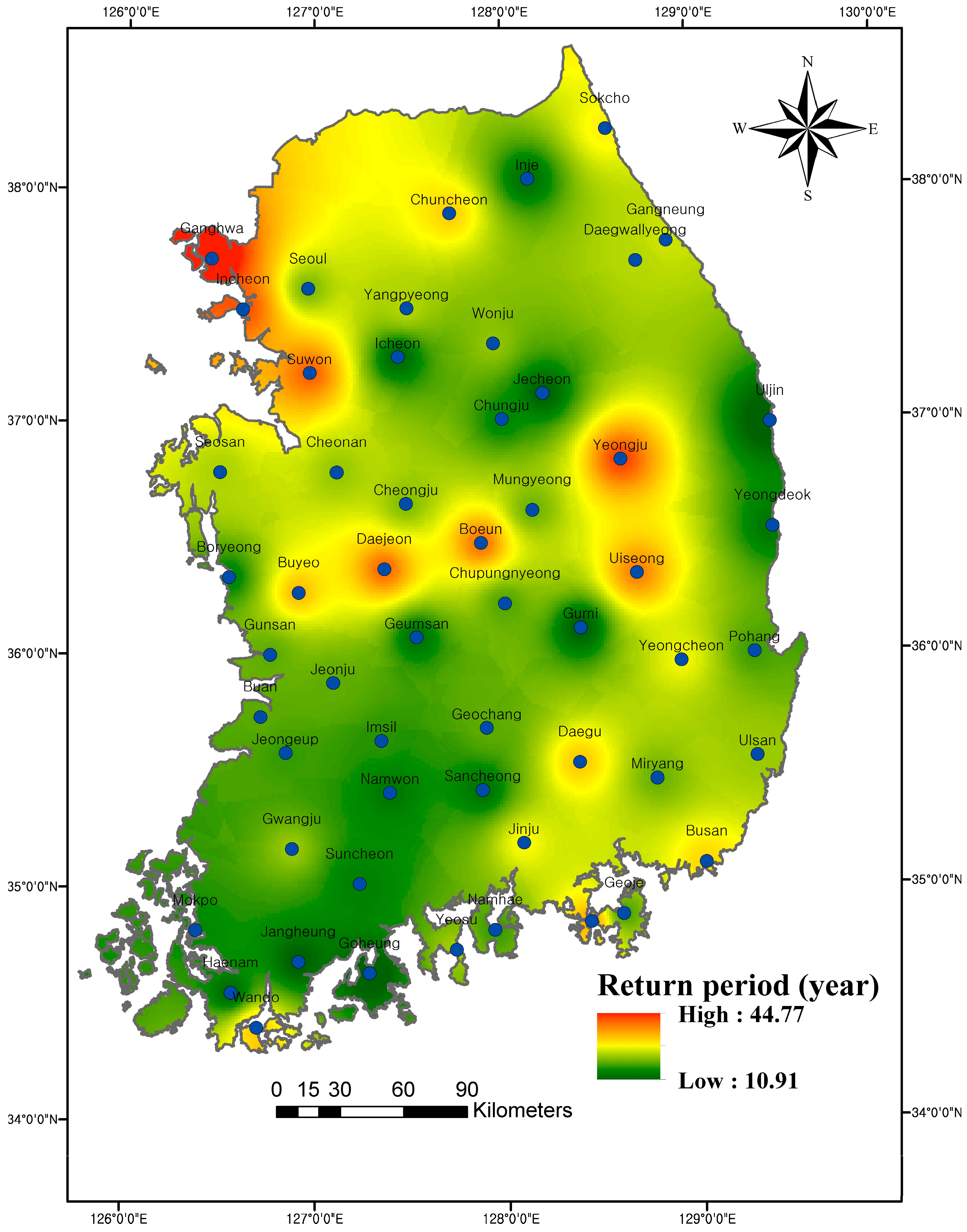
To analyze the supercritical risk of drought characteristics, the Kendall () return period was computed using Equation (7), and the results are shown in Figure 7. The average of the Kendall return period was 27.84 years, which is lower than the average of the “and” return period (35.28 years) and higher than the average of the “or” return period (18.06 years). Meanwhile, the minimum and maximum of the Kendall return period was 10.91 years at Jangheung station and 44.7 years at Ganghwa station. The spatial distribution patterns of secondary (Kendall) return periods () (Figure 7) and primary return periods (,) (Figure 5 and Figure 6) were the same. Overall, the Kendall return period showed droughts of longer duration and higher severities compared with the “or” return periods, and droughts of shorter duration and lower severities compared with the “and” return periods.
3.5. Comparison of Return Periods Using Identified Drought Events
In drought frequency analysis, the droughts of longer duration and higher severities have obtained more importance because they pose high risks for designing and planning of water resource structures. Therefore, based on the SPI (time scale of six months) analysis, 20 long-lasting historical drought events were selected, and their univariate and bivariate return periods were compared using the best fitted marginal distributions (Figure 2a,b) and best fitted copulas (Figure 4). The results are shown in Table 7. The droughts events across 55 rainfall stations are sorted according to their durations only. Drought events are not sorted according to severities because the droughts of longer durations mostly corresponded to the droughts of higher severities. This can be observed from the drought characteristics in Table 3. Besides, a strong correlation between drought duration and severity values also shows that the increase in duration also leads to the increase in the values of severity. Correlation between drought duration and severities can be observed from Table 6. The longest drought (#1) lasted for 13 months from April 2008–April 2009 at Jecheon rainfall station with a drought severity of 16.04. This is because of the non-stationary precipitation pattern at Jecheon station [38]. The most severe drought (#2) occurred at Yeongju station and lasted for 12 months from March 1982–February 1983 with a drought severity of 22.30. In addition, from the results shown in Table 7, it is seen that the is always longer than . This is because the probability that two cases occur simultaneously is relatively smaller than that when one of the two cases occurs. Moreover, it can be noticed from Table 7 that the secondary return period is always larger than the and shorter than . The analysis showed that the difference between Kendall’s return period and the standard return period increased with an increase in the critical probability level t.
It should be noted that according to the method of computation, Kendall’s (secondary) return period () is totally different from the primary return periods () as they explain different situations. Therefore, it is hard to say which type of return period is able to perform consistently better than the other [39]. The preference of the return period changes based on which one better explains the assessment and management requirements of drought risk for the area under study.
4. Conclusions
This study has attempted to investigate the spatio-temporal changes in droughts in South Korea during 1980–2015, using the regional drought frequency analysis approach. Based on the SPI truncation level method, drought duration and severity were extracted at 55 rainfall stations. A Mann–Kendall trend test was used to identify the trends in drought characteristics. The ten most commonly-applied marginal distributions were considered and evaluated using the goodness of fit RMSE and KS test statistics. The best fitted marginal distributions were further evaluated using the visual comparison between empirical and theoretical cumulative probabilities. The dependence relation between two drought variables was tested using Pearson’s correlation measure. For the construction of joint distribution, six copulas were considered, and the best fitted copulas were chosen on the basis of goodness of fit test statistics (Sn, AIC) and the probability-probability plot. The spatial distribution of potential drought risk across South Korea was presented by the “and” and “or” types of joint return periods. In addition, the new concept of Kendall’s return period was also employed and compared with primary return periods. The primary conclusions determined from this study are as follows:
- (1)
- Drought characteristics on the basis of SPI indicate that due to the unusual precipitation pattern in the southwest coastal areas, Jecheon station faced the drought of longest duration and greater severity among 55 stations across South Korea.
- (2)
- Based on the KS test, RMSE and graphical comparison applied to 55 stations, four models (exp, wei, gpa and pe3) were best fitted for drought duration and seven models (wei, ln3, gpa, gno, glo, exp, and pe3) for drought severity. Pe3 is the most common model existing in both drought duration and severity. Based on Sn, AIC and the probability-probability plot, the choice of copula varies from station to station. In addition, the Frank copula is the most common best fitted copula among 55 stations. It is concluded that several different measures are necessary to identify the best fit marginal distributions and copulas. Since different measures reflect different characteristics of marginal distributions and copulas, a single measure may lead to under- or over-estimation of the probability of drought.
- (3)
- The properties of the spatial distributions of , and are the same. However, showed droughts of longer durations and higher severities compared to and droughts of shorter durations and lower severities compared to . The spatial distribution of the joint return period indicates that the southwestern coast of South Korea and surrounding areas of Uljin have a high risk of drought, while the northwestern portion and surrounding areas of Yeongju, Uiseong, Boeun and Daejeon stations have a relatively low risk of drought. The results indicate the serious challenge in the water resource management and human mitigation of drought hazards in the southwestern coast due to abrupt changes in the precipitation pattern. In order to cope with drought hazards, accurate hydrological regulations of reservoirs in the southwest coast is necessary.
- (4)
- The comparison of univariate and bivariate return periods using the top twenty drought events showed, as can be noticed from Table 7, that the secondary return period is always larger than the and shorter than . It is also concluded that the Kendall return period and primary return periods cannot be interchanged, as their applicability changes according to the type of drought risk considered.
Acknowledgments
This research was supported by a grant (11-TI-C06) from the Advanced Water Management Research Program funded by the Ministry of Land, Infrastructure and Transport of the Korean government.
Author Contributions
All of the authors contributed to the conception and development of this manuscript. Muhammad Azam designed, carried out the analysis and wrote the paper. Seung Jin Maeng reviewed and edited the manuscript. Hyung San Kim and Ju Ha Hwang provided assistance in the calculations.
Conflicts of Interest
The authors declare no conflicts of interest.
References
- Choi, G.; Kwon, W.-T.; Boo, K.-O.; Cha, Y.-M. Recent Spatial and Temporal Changes in Means and Extreme Events of Temperature and Precipitation across the Republic of Korea *. J. Korean Geogr. Soc. 2008, 43, 681–700. [Google Scholar]
- Jo, H.K. Impacts of urban greenspace on offsetting carbon emissions for middle Korea. J. Environ. Manag. 2002, 64, 115–126. [Google Scholar] [CrossRef]
- Boo, K.-O.; Kwon, W.-T.; Oh, J.-H.; Baek, H.-J. Response of global warming on regional climate change over Korea: An experiment with the MM5 model. Geophys. Res. Lett. 2004, 31. [Google Scholar] [CrossRef]
- Lee, J.-H.; Seo, J.-W.; Kim, C.-J. Analysis on Trends, Periodicities and Frequencies of Korean Drought Using Drought Indices. J. Korea Water Resour. Assoc. 2012, 45, 75–89. [Google Scholar] [CrossRef]
- Sawada, Y.; Koike, T.; Jaranilla-Sanchez, P.A. Modeling hydrologic and ecologic responses using a new eco-hydrological model for identification of droughts. Water Resour. Res. 2014, 50, 6214–6235. [Google Scholar] [CrossRef]
- Jaranilla-Sanchez, P.A.; Wang, L.; Koike, T. Modeling the hydrologic responses of the Pampanga River basin, Philippines: A quantitative approach for identifying droughts. Water Resour. Res. 2011, 47. [Google Scholar] [CrossRef]
- Mo, K.C.; Lettenmaier, D.P. Objective Drought Classification Using Multiple Land Surface Models. J. Hydrometeorol. 2014, 15, 990–1010. [Google Scholar] [CrossRef]
- Soulé, P.T. Spatial patterns of drought frequency and duration in the contiguous USA based on multiple drought event definitions. Int. J. Climatol. 1992, 12, 11–24. [Google Scholar] [CrossRef]
- Zhao, P.; Lü, H.; Fu, G.; Zhu, Y.; Su, J.; Wang, J. Uncertainty of Hydrological Drought Characteristics with Copula Functions and Probability Distributions: A Case Study of Weihe River, China. Water 2017, 9, 334. [Google Scholar] [CrossRef]
- Yevjevich, V. An Objective Approach to Definitions and Investigations of Continental Hydrologic Droughts; Colorado State University: Fort Collins, CO, USA, 1967. [Google Scholar]
- Yue, S. Applying Bivariate Normal Distribution to Flood Frequency Analysis. Water Int. 1999, 24, 248–254. [Google Scholar] [CrossRef]
- Bacchi, B.; Becciu, G.; Kottegoda, N.T. Bivariate exponential model applied to intensities and durations of extreme rainfall. J. Hydrol. 1994, 155, 225–236. [Google Scholar] [CrossRef]
- Yue, S.; Ouarda, T.B.M.J.; Bobée, B. A review of bivariate gamma distributions for hydrological application. J. Hydrol. 2001, 246, 1–18. [Google Scholar] [CrossRef]
- Azam, M.; Kim, H.S.; Maeng, S.J. Development of flood alert application in Mushim stream watershed Korea. Int. J. Disaster Risk Reduct. 2017, 21, 11–26. [Google Scholar] [CrossRef]
- Kim, H.; Muhammad, A.; Maeng, S.-J. Hydrologic Modeling for Simulation of Rainfall-Runoff at Major Control Points of Geum River Watershed. Procedia Eng. 2016, 154, 504–512. [Google Scholar] [CrossRef]
- Ganguli, P.; Reddy, M.J. Evaluation of trends and multivariate frequency analysis of droughts in three meteorological subdivisions of western India. Int. J. Climatol. 2014, 34, 911–928. [Google Scholar] [CrossRef]
- Cancelliere, A.; Salas, J.D. Drought length properties for periodic-stochastic hydrologic data. Water Resour. Res. 2004, 40. [Google Scholar] [CrossRef]
- Shiau, J.T. Fitting Drought Duration and Severity with Two-Dimensional Copulas. Water Resour. Manag. 2006, 20, 795–815. [Google Scholar] [CrossRef]
- Kim, T.-W.; Valdés, J.B.; Yoo, C. Nonparametric Approach for Estimating Return Periods of Droughts in Arid Regions. J. Hydrol. Eng. 2003, 8, 237–246. [Google Scholar] [CrossRef]
- Hao, Z.; Singh, V. Entropy-based method for bivariate drought analysis. J. Hydrol. Eng. 2012, 18, 780–786. [Google Scholar] [CrossRef]
- Sklar, A. Fonctions de Répartition à n Dimensions et Leurs Marges; Institut de Statistique de L’Université de Paris: Paris, France, 1959; Volume 8, pp. 229–231. (In French) [Google Scholar]
- Wang, Y.; Li, C.; Liu, J.; Yu, F.; Qiu, Q.; Tian, J.; Zhang, M. Multivariate Analysis of Joint Probability of Different Rainfall Frequencies Based on Copulas. Water 2017, 9, 198. [Google Scholar] [CrossRef]
- Nelsen, R.B. An Introduction to Copulas; Springer Science & Business Media: Berlin, Germany, 2013; Volume 53, ISBN 9788578110796. [Google Scholar]
- Marsaglia, G.; Marsaglia, J. Evaluating the anderson-darling distribution. J. Stat. Softw. 2004, 9, 1–5. [Google Scholar] [CrossRef]
- Kim, J.-S.; Jain, S. Precipitation trends over the Korean peninsula: Typhoon-induced changes and a typology for characterizing climate-related risk. Environ. Res. Lett. 2011, 6, 34033. [Google Scholar] [CrossRef]
- Mckee, T.B.; Doesken, N.J.; Kleist, J. The relationship of drought frequency and duration to time scales. In Proceedings of the Eighth Conference on Applied Climatology, Anaheim, CA, USA, 17–22 January 1993; pp. 179–184. [Google Scholar]
- Mishra, A.K.; Singh, V.P. Drought modeling—A review. J. Hydrol. 2011, 403, 157–175. [Google Scholar] [CrossRef]
- Xu, K.; Yang, D.; Xu, X.; Lei, H. Copula based drought frequency analysis considering the spatio-temporal variability in Southwest China. J. Hydrol. 2015, 527, 630–640. [Google Scholar] [CrossRef]
- Genest, C.; Rémillard, B.; Beaudoin, D. Goodness-of-fit tests for copulas: A review and a power study. Insur. Math. Econ. 2009, 44, 199–213. [Google Scholar] [CrossRef]
- Requena, A.I.; Chebana, F.; Mediero, L. A complete procedure for multivariate index-flood model application. J. Hydrol. 2016, 535, 559–580. [Google Scholar] [CrossRef]
- Salvadori, G.; De Michele, C.; Durante, F. On the return period and design in a multivariate framework. Hydrol. Earth Syst. Sci. 2011, 15, 3293–3305. [Google Scholar] [CrossRef] [Green Version]
- Shiau, J.T.; Feng, S.; Nadarajah, S. Assessment of hydrological droughts for the Yellow River, China, using copulas. Hydrol. Process. 2007, 21, 2157–2163. [Google Scholar] [CrossRef]
- Shiau, J.T. Return period of bivariate distributed extreme hydrological events. Stoch. Environ. Res. Risk Assess. 2003, 17, 42–57. [Google Scholar] [CrossRef]
- Salvadori, G.; De Michele, C. Multivariate multiparameter extreme value models and return periods: A copula approach. Water Resour. Res. 2010, 46. [Google Scholar] [CrossRef]
- Vandenberghe, S.; Verhoest, N.E.C.; Onof, C.; De Baets, B. A comparative copula-based bivariate frequency analysis of observed and simulated storm events: A case study on Bartlett-Lewis modeled rainfall. Water Resour. Res. 2011, 47. [Google Scholar] [CrossRef]
- Salvadori, G.; De Michele, C. Frequency analysis via copulas: Theoretical aspects and applications to hydrological events. Water Resour. Res. 2004, 40. [Google Scholar] [CrossRef]
- Genest, C.; Favre, A.-C. Everything You Always Wanted to Know about Copula Modeling but Were Afraid to Ask. J. Hydrol. Eng. 2007, 12, 347–368. [Google Scholar] [CrossRef]
- Park, J.-S.; Kang, H.-S.; Lee, Y.S.; Kim, M.-K. Changes in the extreme daily rainfall in South Korea. Int. J. Climatol. 2011, 31, 2290–2299. [Google Scholar] [CrossRef]
- Serinaldi, F. Dismissing return periods! Stoch. Environ. Res. Risk Assess. 2015, 29, 1179–1189. [Google Scholar] [CrossRef]
Figure 1.
Comparison between empirical and theoretical CDFs for the Jecheon rainfall station: (a) drought duration (months); (b) drought severity.
Figure 1.
Comparison between empirical and theoretical CDFs for the Jecheon rainfall station: (a) drought duration (months); (b) drought severity.
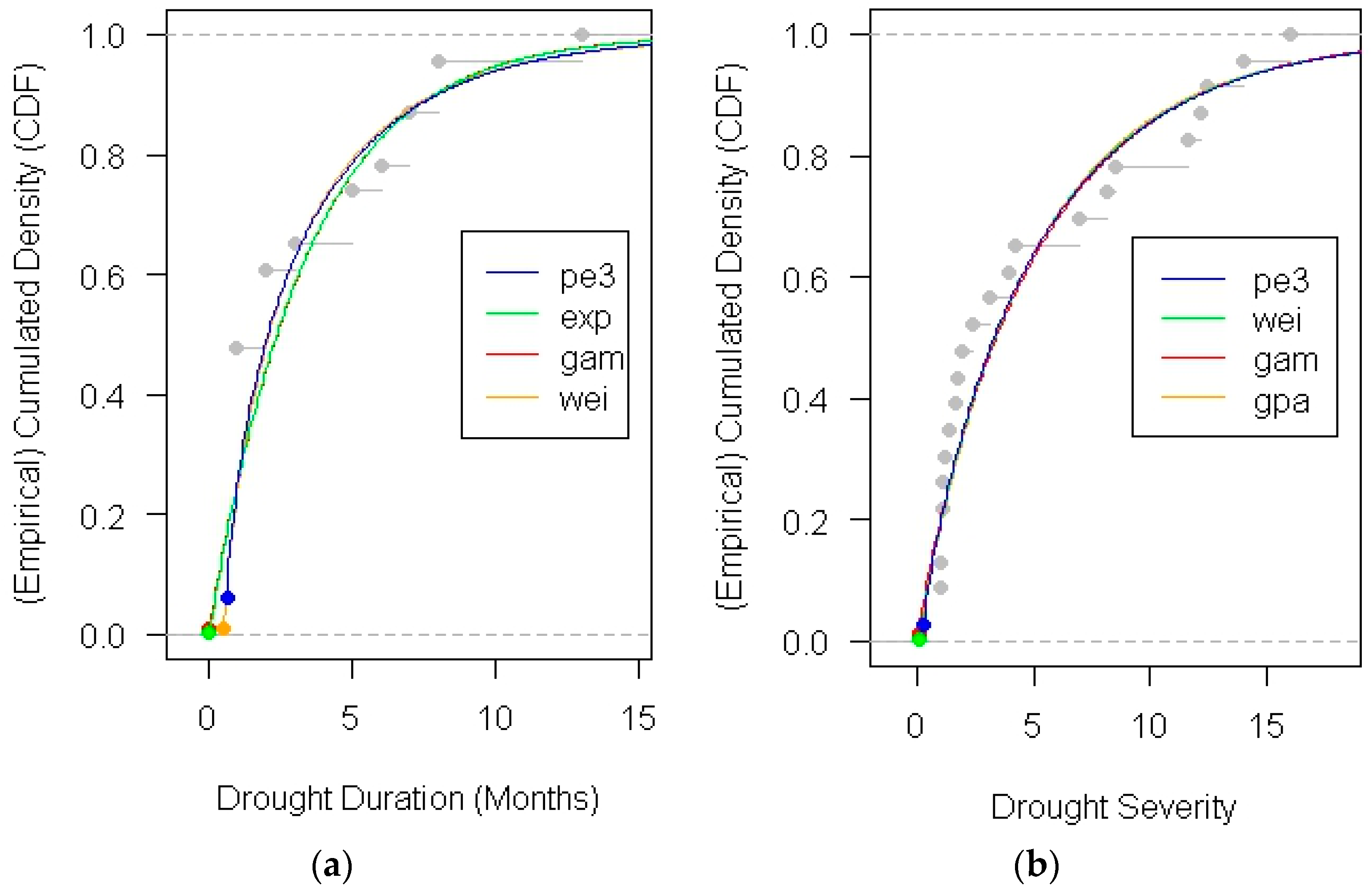
Figure 2.
Selected best fitted marginal distributions of drought duration and severity for each rainfall station. (a) Drought duration; (b) drought severity.
Figure 2.
Selected best fitted marginal distributions of drought duration and severity for each rainfall station. (a) Drought duration; (b) drought severity.
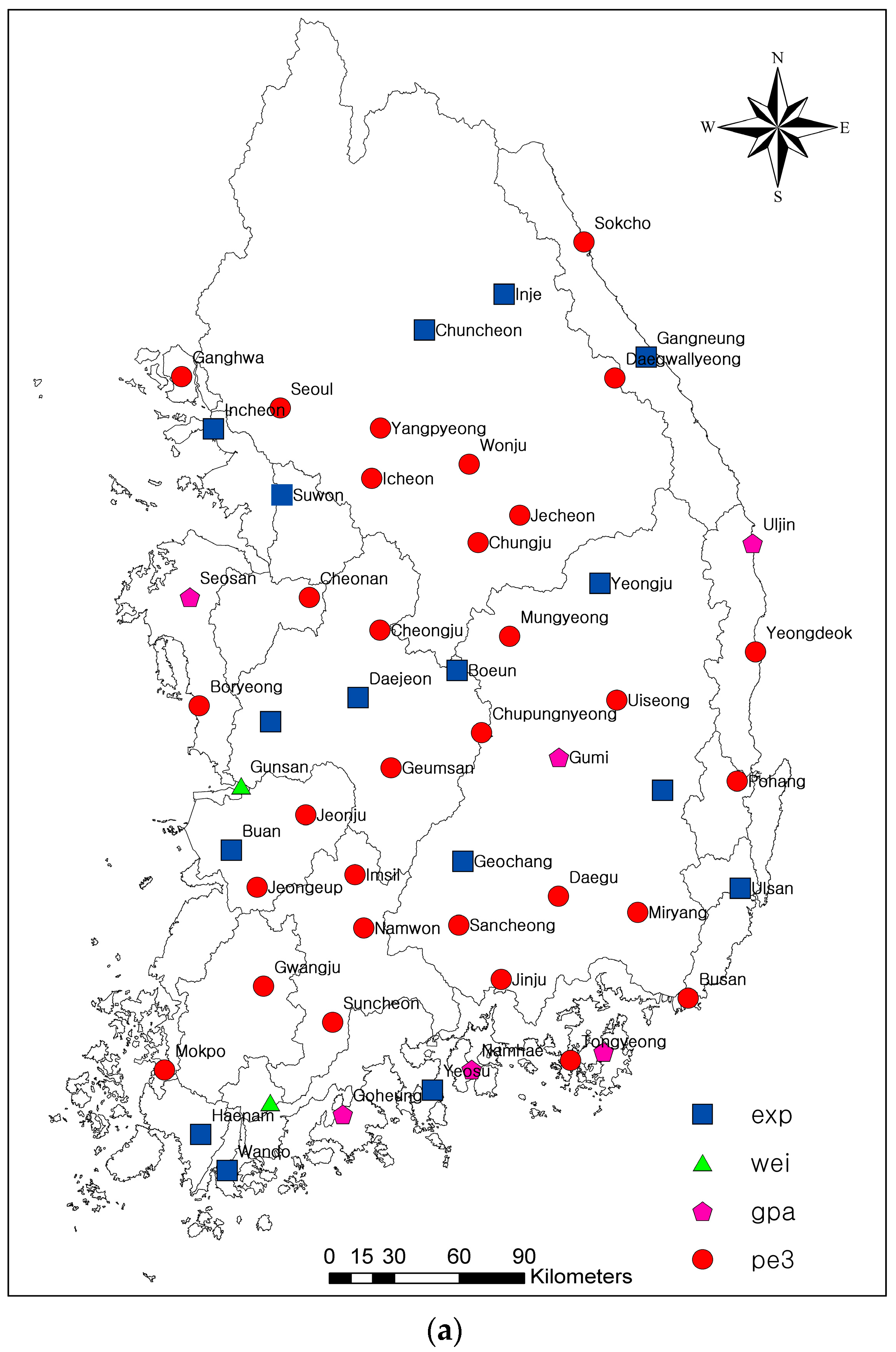

Figure 3.
Probability-probability (PP) plot of the bivariate copulas at Jecheon rainfall station.

Figure 4.
Best fitted bivariate copula for each rainfall station.

Figure 5.
Spatial distribution of the bivariate return period under the condition D ≥ d ∧ S ≥ s across South Korea.
Figure 5.
Spatial distribution of the bivariate return period under the condition D ≥ d ∧ S ≥ s across South Korea.
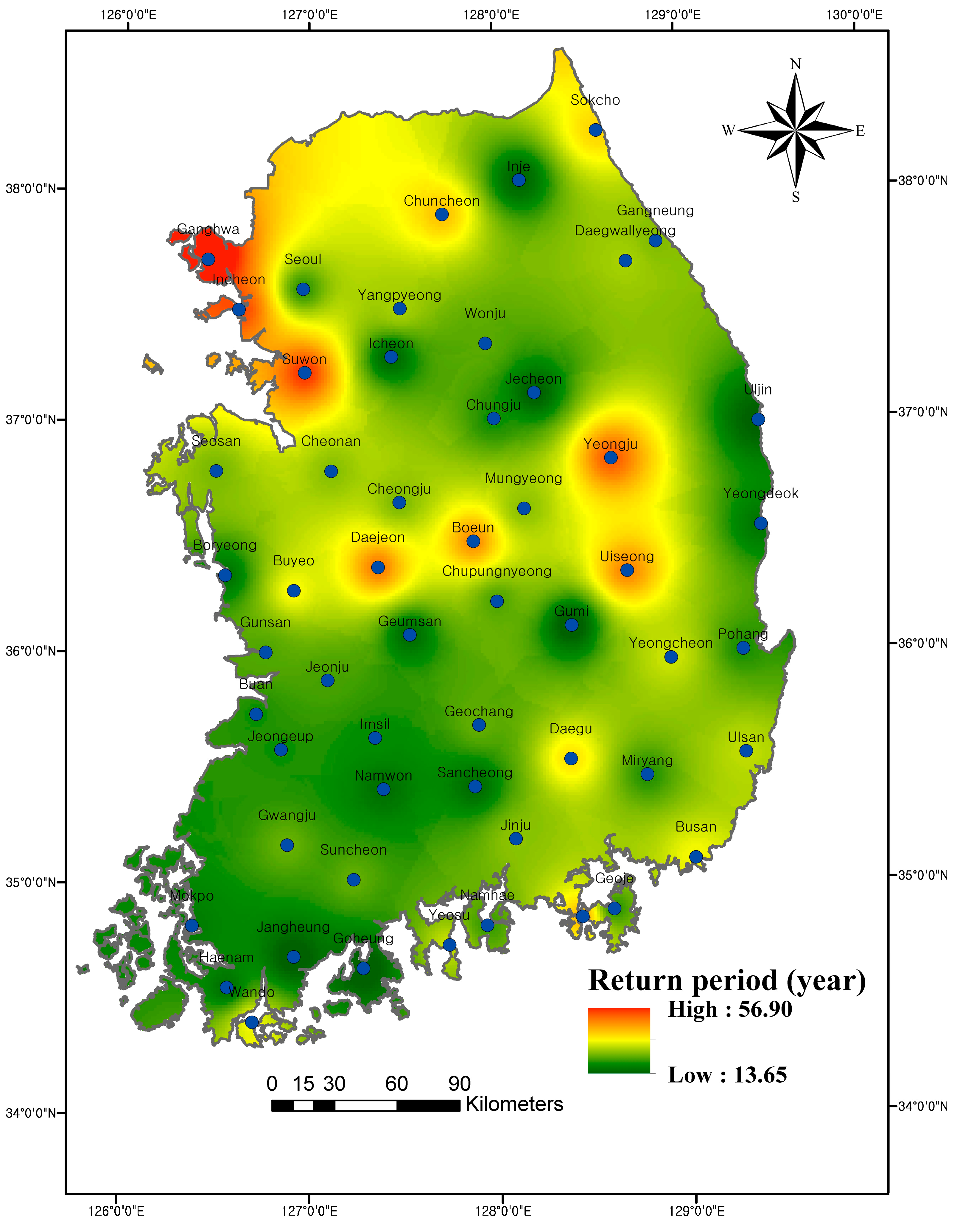
Figure 6.
Spatial distribution of the bivariate return period under the condition of D ≥ d ∨ S ≥ s across South Korea.
Figure 6.
Spatial distribution of the bivariate return period under the condition of D ≥ d ∨ S ≥ s across South Korea.
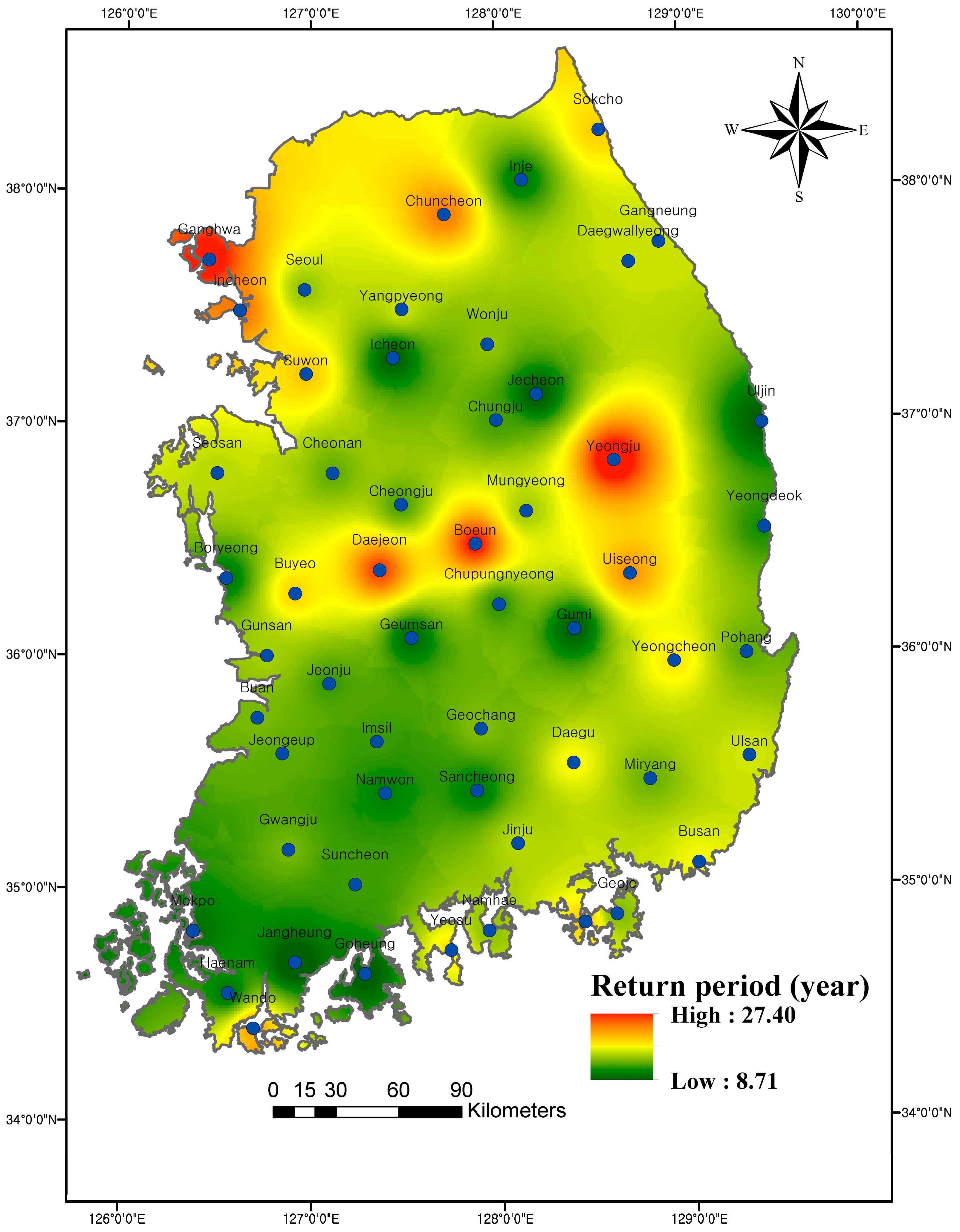
Figure 7.
Spatial distribution of the bivariate Kendall return period.

Table 1.
List of copulas used in this study.
| Copulas | Bivariate Copula | Parameters |
|---|---|---|
| Archimedean copulas | ||
| Clayton | ||
| Frank | ||
| Gumbel | ||
| Joe | ||
| Elliptical copulas | ||
| Student’s t | where | |
| Gaussian | ||
Table 2.
List of probability distributions used in this study.
| Distribution | CDF | Parameters |
|---|---|---|
| Exponential (exp) | , | |
| Gamma (gam) | , | |
| Generalized extreme value (gev) | , , | |
| Generalized logistic (glo) | , , | |
| generalized normal (gno) | , , | |
| Generalized Pareto (gpa) | , , | |
| Gumbel (gum) | , | |
| Lognormal (ln3) | , , | |
| Pearson Type 3 (pe3) | , | |
| Weibull (wei) | , |
Table 3.
Characteristics of drought during 1980–2015 at 55 rainfall stations.
| Station | Drought Events | M.D | M.S | Mx | Station | Drought Events | M.D | M.S | Mx |
|---|---|---|---|---|---|---|---|---|---|
| Sokcho | 29 | 2.31 | 3.37 | 9 | Ganghwa | 24 | 2.17 | 3.51 | 11 |
| Daegwallyeong | 28 | 2.36 | 3.31 | 9 | Yangpyeong | 28 | 2.46 | 3.65 | 9 |
| Chuncheon | 31 | 2.29 | 3.35 | 8 | Icheon | 21 | 2.90 | 4.66 | 7 |
| Gangneung | 29 | 2.45 | 3.55 | 7 | Inje | 24 | 2.96 | 4.33 | 8 |
| Seoul | 24 | 2.79 | 4.18 | 10 | Jecheon | 23 | 3.43 | 5.14 | 13 |
| Incheon | 32 | 2.19 | 3.16 | 10 | Boeun | 29 | 2.31 | 3.43 | 8 |
| Wonju | 24 | 2.50 | 4.08 | 8 | Cheonan | 28 | 2.32 | 3.50 | 7 |
| Suwon | 26 | 2.38 | 3.63 | 7 | Boryeong | 29 | 2.69 | 4.12 | 7 |
| Chungju | 27 | 2.59 | 3.90 | 7 | Buyeo | 30 | 2.37 | 3.46 | 8 |
| Seosan | 28 | 2.61 | 3.82 | 6 | Geumsan | 30 | 2.77 | 4.11 | 8 |
| Uljin | 25 | 2.92 | 4.16 | 6 | Buan | 30 | 2.70 | 3.98 | 10 |
| Cheongju | 27 | 2.52 | 3.99 | 7 | Imsil | 26 | 2.85 | 4.54 | 9 |
| Daejeon | 31 | 2.26 | 3.40 | 7 | Jeongeup | 30 | 2.63 | 3.83 | 9 |
| Chupungnyeong | 28 | 2.57 | 3.90 | 9 | Namwon | 25 | 2.80 | 4.57 | 9 |
| Pohang | 16 | 2.06 | 2.85 | 6 | Jangheung | 23 | 3.35 | 5.03 | 8 |
| Gunsan | 25 | 2.68 | 4.14 | 9 | Haenam | 26 | 2.58 | 3.84 | 8 |
| Daegu | 29 | 2.17 | 3.52 | 7 | Goheung | 21 | 3.29 | 5.12 | 9 |
| Jeonju | 28 | 2.64 | 4.21 | 8 | Yeongju | 29 | 2.38 | 3.68 | 12 |
| Ulsan | 27 | 2.52 | 3.80 | 8 | Mungyeong | 27 | 2.44 | 3.79 | 10 |
| Gwangju | 26 | 2.58 | 4.06 | 8 | Yeongdeok | 24 | 2.83 | 4.20 | 9 |
| Busan | 31 | 2.00 | 2.95 | 7 | Uiseong | 29 | 2.00 | 3.33 | 8 |
| Tongyeong | 33 | 1.97 | 2.78 | 7 | Gumi | 24 | 3.17 | 4.74 | 9 |
| Mokpo | 20 | 2.80 | 4.65 | 8 | Yeongcheon | 24 | 2.58 | 4.07 | 8 |
| Yeosu | 30 | 2.53 | 3.73 | 8 | Geochang | 24 | 2.88 | 4.65 | 10 |
| Wando | 21 | 3.05 | 4.69 | 9 | Miryang | 27 | 2.93 | 4.35 | 10 |
| Suncheon | 27 | 2.56 | 3.92 | 10 | Sancheong | 21 | 3.00 | 4.97 | 9 |
| Jinju | 28 | 2.61 | 4.01 | 9 | Geoje | 24 | 2.67 | 3.89 | 7 |
| Namhae | 24 | 2.63 | 4.19 | 8 | |||||
| Average | 2.60 | 3.96 | 8.40 |
Note: “M.D” indicates mean drought duration, “M.S” indicates corresponding mean drought severity, “Mx” indicates drought event of longest duration in months.
Table 4.
Parameters and goodness of fit of the marginal distribution at Jecheon rainfall station.
| Drought Duration | Drought Severity | |||||||
|---|---|---|---|---|---|---|---|---|
| Distribution | Parameters | RMSE | KS Test | Parameters | RMSE | KS Test | ||
| Statistic | p-Value | Statistic | p-Value | |||||
| exp | ξ = 0.04 | 0.173 | 0.247 | 0.121 | ξ = −0.21 | 0.082 | 0.208 | 0.274 |
| α = 3.40 | α = 5.33 | |||||||
| gam | α = 1.03 | 0.174 | 0.247 | 0.122 | α = 0.90 | 0.079 | 0.205 | 0.287 |
| β = 3.34 | β = 5.70 | |||||||
| gev | ξ = 1.70 | 0.212 | 0.290 | 0.042 | ξ = 2.49 | 0.098 | 0.192 | 0.367 |
| α = 1.51 | α = 2.72 | |||||||
| κ = −0.37 | κ = −0.29 | |||||||
| glo | ξ = 2.33 | 0.215 | 0.292 | 0.040 | ξ = 3.61 | 0.104 | 0.202 | 0.305 |
| α = 1.22 | α = 2.11 | |||||||
| κ = −0.43 | κ = −0.37 | |||||||
| gno | ξ = 2.22 | 0.200 | 0.275 | 0.061 | ξ = 3.45 | 0.090 | 0.176 | 0.407 |
| α = 2.10 | α = 3.66 | |||||||
| κ = −0.93 | κ = −0.08 | |||||||
| gpa | ξ = 0.39 | 0.189 | 0.259 | 0.091 | ξ = −0.01 | 0.080 | 0.195 | 0.346 |
| α = 2.42 | α = 4.73 | |||||||
| κ = −0.21 | κ = −0.07 | |||||||
| gum | ξ = 2.02 | 0.202 | 0.259 | 0.092 | ξ = 2.90 | 0.110 | 0.205 | 0.289 |
| α = 2.45 | α = 3.84 | |||||||
| ln3 | ζ = −0.05 | 0.200 | 0.275 | 0.061 | ζ = −1.24 | 0.090 | 0.202 | 0.305 |
| µ = 0.82 | µ = 1.55 | |||||||
| σ = 0.93 | σ = 0.78 | |||||||
| pe3 | ξ = 2.43 | 0.170 | 0.244 | 0.129 | ξ = 5.12 | 0.077 | 0.176 | 0.472 |
| β = 3.67 | β = 5.47 | |||||||
| α = 2.61 | α = 2.22 | |||||||
| wei | ζ = −0.54 | 0.179 | 0.246 | 0.123 | ζ = −0.11 | 0.078 | 0.199 | 0.324 |
| β = 2.52 | β = 2.52 | |||||||
| δ = 0.78 | δ = 0.78 | |||||||
Table 5.
Parameters and goodness of fit of the copula at Jecheon rainfall station.
| Copula | Sn | p-Value | AIC | θ |
|---|---|---|---|---|
| Student’s t | 0.023 | 0.203 | 69.989 | 0.989 |
| Normal | 0.030 | 0.035 | 84.973 | 0.989 |
| Clayton | 0.033 | 0.124 | 86.223 | 11.024 |
| Gumbel | 0.022 | 0.391 | 68.996 | 8.872 |
| Frank | 0.031 | 0.054 | 80.005 | 38.072 |
| Joe | 0.024 | 0.104 | 79.259 | 11.493 |
Table 6.
Pearson correlation for the drought duration and severity at 55 rainfall stations.
| Station | Correlation | p-Value | Station | Correlation | p-Value |
|---|---|---|---|---|---|
| Sokcho | 0.984 | 9.5 × 10⁻²² | Ganghwa | 0.988 | 2.9 × 10⁻¹⁹ |
| Daegwallyeong | 0.979 | 1.2 × 10⁻¹⁹ | Yangpyeong | 0.978 | 3.0 × 10⁻¹⁹ |
| Chuncheon | 0.973 | 4.5 × 10⁻²⁰ | Icheon | 0.968 | 6.5 × 10⁻¹³ |
| Gangneung | 0.981 | 1.0 × 10⁻²⁰ | Inje | 0.995 | 4.6 × 10⁻²³ |
| Seoul | 0.994 | 2.6 × 10⁻²² | Jecheon | 0.977 | 1.2 × 10⁻¹⁵ |
| Incheon | 0.961 | 2.7 × 10⁻¹⁸ | Boeun | 0.983 | 1.4 × 10⁻²¹ |
| Wonju | 0.987 | 7.2 × 10⁻¹⁹ | Cheonan | 0.966 | 8.3 × 10⁻¹⁷ |
| Suwon | 0.946 | 2.9 × 10⁻¹³ | Boryeong | 0.970 | 4.6 × 10⁻¹⁸ |
| Chungju | 0.983 | 4.8 × 10⁻²⁰ | Buyeo | 0.975 | 6.5 × 10⁻²⁰ |
| Seosan | 0.971 | 1.0 × 10⁻¹⁷ | Geumsan | 0.977 | 2.4 × 10⁻²⁰ |
| Uljin | 0.976 | 1.0 × 10⁻¹⁶ | Buan | 0.987 | 6.2 × 10⁻²⁴ |
| Cheongju | 0.965 | 4.4 × 10⁻¹⁶ | Imsil | 0.974 | 4.8 × 10⁻¹⁷ |
| Daejeon | 0.974 | 3.2 × 10⁻²⁰ | Jeongeup | 0.988 | 3.1 × 10⁻²⁴ |
| Chupungnyeong | 0.972 | 5.9 × 10⁻¹⁸ | Namwon | 0.985 | 4.3 × 10⁻¹⁹ |
| Pohang | 0.985 | 5.4 × 10⁻¹² | Jangheung | 0.965 | 1.0 × 10⁻¹³ |
| Gunsan | 0.985 | 6.3 × 10⁻¹⁹ | Haenam | 0.975 | 3.4 × 10⁻¹⁷ |
| Daegu | 0.971 | 3.1 × 10⁻¹⁸ | Goheung | 0.966 | 1.3 × 10⁻¹² |
| Jeonju | 0.968 | 4.1 × 10⁻¹⁷ | Yeongju | 0.991 | 4.9 × 10⁻²⁵ |
| Ulsan | 0.972 | 3.2 × 10⁻¹⁷ | Mungyeong | 0.985 | 9.6 × 10⁻²¹ |
| Gwangju | 0.976 | 2.6 × 10⁻¹⁷ | Yeongdeok | 0.989 | 7.5 × 10⁻²⁰ |
| Busan | 0.980 | 9.6 × 10⁻²² | Uiseong | 0.988 | 2.9 × 10⁻²³ |
| Tongyeong | 0.981 | 3.1 × 10⁻²⁴ | Gumi | 0.990 | 2.6 × 10⁻²⁰ |
| Mokpo | 0.985 | 2.7 × 10⁻¹⁵ | Yeongcheon | 0.970 | 5.7 × 10⁻¹⁵ |
| Yeosu | 0.971 | 7.3 × 10⁻¹⁹ | Geochang | 0.972 | 2.4 × 10⁻¹⁵ |
| Wando | 0.982 | 3.4 × 10⁻¹⁵ | Miryang | 0.990 | 6.6 × 10⁻²³ |
| Suncheon | 0.988 | 1.3 × 10⁻²¹ | Sancheong | 0.968 | 7.6 × 10⁻¹³ |
| Jinju | 0.977 | 6.1 × 10⁻¹⁹ | Geoje | 0.966 | 2.2 × 10⁻¹⁴ |
| Namhae | 0.986 | 1.4 × 10⁻¹⁸ |
Table 7.
Comparison of univariate and bivariate return periods using the top twenty drought events.
| # 1 | Station | Date | D 1 | S 1 | 1 | 1 | 1 | 1 | 1 |
|---|---|---|---|---|---|---|---|---|---|
| 1 | Jecheon | April 2008~April 2009 | 13 | 16.04 | 33.53 | 19.79 | 34.81 | 19.39 | 22.22 |
| 2 | Yeongju | March 1982~February 1983 | 12 | 22.30 | 62.65 | 68.10 | 78.27 | 55.96 | 69.51 |
| 3 | Ganghwa | March 2014~January 2015 | 11 | 20.01 | 41.55 | 48.56 | 63.49 | 34.59 | 45.89 |
| 4 | Geochang | July 2008~April 2009 | 10 | 21.50 | 44.58 | 57.40 | 165.38 | 29.58 | 86.51 |
| 5 | Suncheon | April 1988~January 1989 | 10 | 16.98 | 21.41 | 17.41 | 23.18 | 16.39 | 18.79 |
| 6 | Miryang | April 1988~January 1989 | 10 | 16.46 | 27.63 | 29.91 | 62.36 | 18.66 | 44.06 |
| 7 | Mungyeong | March 1982~December 1982 | 10 | 16.15 | 35.96 | 35.99 | 44.37 | 30.25 | 39.46 |
| 8 | Buan | April 1988~January 1989 | 10 | 16.00 | 60.95 | 44.97 | 370.57 | 27.82 | 194.56 |
| 9 | Seoul | March 2014~December 2014 | 10 | 15.44 | 29.42 | 25.48 | 57.26 | 17.93 | 40.12 |
| 10 | Incheon | March 2014~December 2014 | 10 | 12.94 | 51.67 | 31.50 | 149.37 | 22.52 | 79.45 |
| 11 | Namwon | May 1994~January 1995 | 9 | 20.55 | 27.05 | 37.45 | 134.63 | 17.78 | 79.61 |
| 12 | Jinju | June 1994~February 1995 | 9 | 17.61 | 31.02 | 39.77 | 96.66 | 21.26 | 63.71 |
| 13 | Imsil | April 1995~December 1995 | 9 | 17.41 | 25.26 | 28.63 | 33.81 | 22.25 | 26.45 |
| 14 | Daegwallyeong | April 2015~December 2015 | 9 | 16.16 | 35.70 | 46.99 | 54.69 | 32.25 | 45.52 |
| 15 | Chupungnyeong | March 1982~November 1982 | 9 | 15.54 | 26.49 | 38.04 | 96.25 | 18.64 | 63.54 |
| 16 | Wando | June 1995~February 1996 | 9 | 14.86 | 34.48 | 26.83 | 34.90 | 26.58 | 31.56 |
| 17 | Sokcho | February 2015~October 2015 | 9 | 14.71 | 32.96 | 34.95 | 67.56 | 22.65 | 39.47 |
| 18 | Jeongeup | April 1994~December 1994 | 9 | 14.58 | 31.99 | 31.82 | 56.82 | 22.18 | 42.01 |
| 19 | Yangpyeong | April 2000~December 2000 | 9 | 13.88 | 31.44 | 26.94 | 121.26 | 16.48 | 61.29 |
| 20 | Gunsan | May 1988~January 1989 | 9 | 13.25 | 28.99 | 23.06 | 29.60 | 22.69 | 25.91 |
Notes: 1 “#” indicates the drought event number; “D” indicates the drought duration measured in months; “S” indicates the drought severity; , , , and are measured in years.
© 2017 by the authors. Licensee MDPI, Basel, Switzerland. This article is an open access article distributed under the terms and conditions of the Creative Commons Attribution (CC BY) license (http://creativecommons.org/licenses/by/4.0/).
Share and Cite
MDPI and ACS Style
Maeng, S.J.; Azam, M.; Kim, H.S.; Hwang, J.H. Analysis of Changes in Spatio-Temporal Patterns of Drought across South Korea. Water 2017, 9, 679. https://doi.org/10.3390/w9090679
AMA Style
Maeng SJ, Azam M, Kim HS, Hwang JH. Analysis of Changes in Spatio-Temporal Patterns of Drought across South Korea. Water. 2017; 9(9):679. https://doi.org/10.3390/w9090679
Chicago/Turabian StyleMaeng, Seung Jin, Muhammad Azam, Hyung San Kim, and Ju Ha Hwang. 2017. "Analysis of Changes in Spatio-Temporal Patterns of Drought across South Korea" Water 9, no. 9: 679. https://doi.org/10.3390/w9090679
Note that from the first issue of 2016, this journal uses article numbers instead of page numbers. See further details here.