Simulating Laboratory Braided Rivers with Bed-Load Sediment Transport

1
Department of Hydraulic Engineering, South China Agricultural University, Guangzhou 510642, China
2
State Key Laboratory of Hydroscience and Engineering, Tsinghua University, Beijing 100084, China
*
Author to whom correspondence should be addressed.
Water 2017, 9(9), 686; https://doi.org/10.3390/w9090686
Submission received: 12 June 2017
/
Revised: 27 August 2017
/
Accepted: 5 September 2017
/
Published: 8 September 2017
Abstract
:Numerical models provide considerable assistance in the investigation of complicated processes in natural rivers. In the present study, a physics-based two-dimensional model has been developed to simulate the braiding processes and morphodynamic changes in braided rivers. The model applies the basic hydrodynamic and sediment transport principles with bed morphology deformation and a TVD (Total Variation Diminishing) scheme to predict trans-critical flows and bed morphology deformation. The non-equilibrium transport process of graded bed load sediment is simulated, with non-uniform sediments, secondary flows, and sheltering effects being included. A multiple bed layer technique is adopted to represent the vertical sediment sorting process. The model has been applied to simulate the bed evolution process in an experimental river with bed load transport. Comparisons between the experimental river and predicted river are analysed, including their pattern evolution processes, important braiding phenomena, and statistical characteristics. Avulsion activities have been found in the braiding evolution process, representing the primary ways in which channels form and disappear in braided rivers. The increases in the active braiding intensity and total braiding intensity show similar trends to those observed in the experimental river. Statistical methods are applied to assess the scale-invariant topographic properties of the simulated river and real rivers. The model demonstrated its potential to predict the morphodynamics in natural rivers.
1. Introduction
Braided rivers are a distinctive river morphology with high flow energy and frequent channel changes. Braiding is one kind of fluvial pattern in these rivers characterized by complex dynamics, in which water and sediment flow are divided into multiple branches, joining and splitting at the nodes and shifting continuously in the floodplain [1]. The understanding of morphodynamics in braided rivers is especially important for managing engineering problems such as flood management, riverbank erosion, sedimentation in reservoirs and navigable waterways, and the design and construction of artificial channels and bridges.
Braiding usually occurs with a highly variable discharge, an abundant sediment load, erodible banks, steep valley slopes, and a high width/depth ratio [2]. A change in one of these parameters might cause an exchange between meandering and braided patterns such as a large flood, an increased sediment supply, a steeper riverbed, or reduced bank erodibility. Ham and Church studied the lower reach of Chilliwack River in Canada, which is partially braided, and found that a large flood with a return period of about five years can be considered a significant channel-forming event [3]. The lower William River in Canada adjusted its channel from a relatively narrow and deep single-channel stream to a thoroughly braided pattern after picking up a 40-fold increase of bed load sediment [4]. The Squamish River experienced a downstream sequence of braided-wandering-meandering in a 20 km reach with a slope decrease from 0.0058 to 0.0015 [5]. Brierley and Hickin studied flow patterns from minimum flow energy and found that meandering rivers may occur even as flow energy has reached the level for braiding, since scouring has been confined by relatively cohesive or vegetated banks [6]. Generally, although one of the factors mentioned above can initiate braided rivers, in nature frequently two or more of them occur simultaneously. Moreover, it is very important to study rivers over an extended time span because their appearance is controlled by the history of changing flow stages, and some geometries arise specially as a result of changing discharge [7].
Numerical models provide useful tools for simulating fluvial processes and morphology in rivers, and, in recent decades, efforts have been made to investigate advanced numerical models to better represent the complex morphodynamic processes in rivers. A few models have been developed to simulate the processes of sediment transport, bed deformation, and sediment downstream fining in rivers (e.g., [8,9,10,11]). Compared with reduced-complexity approaches (e.g., [12,13]), physics-based models provide more detailed process information to better understand natural rivers due to their better representation of hydraulic and morphodynamic processes. Physics-based models have produced braided patterns, bar formation, and avulsion activities observed in natural braided rivers and have made significant progress (e.g., [14,15]). The evolution of wide shallow channels and the behaviour of alternate bars in laboratories have been reproduced by a 2-D model [16,17]. Morphodynamic models such as HSTAR (Hydrodynamics and Sediment Transport in Alluvial Rivers) [18], depth-integrated Delft3D [14,19], and 2-D morphodynamic models [20,21] have been applied to simulate large sand-bed braided rivers and have produced morphological units with evolution mechanisms, the characteristic morphology of compound bars, and channels and statistical characteristics that are similar to those of natural sand-bed rivers. However, their development and application are still in an early stage [22], and quantitative analyses and comparisons between simulated and real rivers are still insufficient [14] especially for braided rivers dominated by bed-load sediment transport.
In braided river simulation, previous models have incorporated basic sediment transport theories with essential effects and have shown considerable potential (e.g., [23,24]). The effect of secondary flow has been integrated into the shallow water equations [18,25] or in the sediment transport rate equation [16,17]. A TVD (Total Variation Diminishing) scheme, which is a modified Ultimate Quickest scheme, has been employed to solve the flow conservation equations (e.g., [23]), since the scheme is more efficient than the implicit ADI (Alternating Direction Implicit) scheme in predicting trans-critical flows that usually exist in shallow areas of braided rivers. Bank erosion, which is important for the emergence of bars and the initiation of meandering or braiding, has been examined theoretically through the mechanical processes of channels [26,27] and has been proposed to reproduce lateral changes by the existing braided river models (e.g., [17,18]).
However, most of the existing physics-based models for braided river simulation adopted a uniform sediment transport approach (e.g., [14,19,28]), except for the model of Nicholas [18] in which two grain fractions of sand and silt were considered. Nevertheless, non-uniform sediments exist in natural rivers, and different size fractions of sediment particles are transported at different rates [29]. Sediment gradation plays an essential role in the bed deformation process, which is especially important for the evolution of local units in natural [30] and laboratory braided rivers [31]. In addition, laboratory experiments [32] also show the influence of vertical grain sorting in the active layer, indicating that it is necessary to divide the riverbed into multiple bed layers in river simulation. This mixing layer concept has been adopted by many researchers such as Wu [29] and Van Niekerk et al. [33]. Therefore, in order to represent a more realistic morphodynamic process in braided rivers, it is necessary for a numerical model to include the effect of non-uniform sediment transport.
In the current study, a 2-D physics-based model has been developed to simulate an experimental river to study the morphodynamics of braided rivers dominated by bed-load sediment. The model incorporates the basic hydrodynamic and sediment transport theories, considers non-uniform sediments in a fractional way, and adopts multiple bed layers to represent the erosion-deposition process and the sorting effects among fractional sediments in beds. The study aims to investigate the river morphodynamic processes and activities, analyse the statistical characteristics, compare them with the experimental river and natural rivers, and discuss the potential of the model for representing the morphodynamic processes in real rivers.
2. Numerical Model and Test
Flow, sediment transport, and bed deformation are normally the main processes considered in river morphodynamic simulations. In the present model, flow and sediment transport are calculated by solving the depth-integrated 2D shallow water equations and the non-equilibrium sediment transport equations.
2.1. Numerical Model
2.1.1. Governing Equations for Flow and Sediment Transport
The flow in rivers is governed by the 2-D shallow water equations, given as follows:
where is the water surface elevation above the datum; and are the discharges per unit of width in the x and y directions, respectively; is the momentum correction factor for a non-uniform vertical velocity profile; and are the depth-averaged velocity components in the and directions, respectively; is the Coriolis parameter due to the Earth’s rotation; is the water depth, which is equal to h + , with h as the water depth below the datum; C is the Chézy coefficient, which equals to , with denoting the hydraulic roughness, given according to van Rijn [34]; and ε is the depth-averaged turbulent eddy viscosity. The hydrodynamic model, which is solved by the TVD-MacCormack Scheme, has been validated in previous studies [35,36], showing its efficiency in simulating trans-critical flows.
Assuming that the graded bed material can be divided into N fractions, the transport of the kth fraction can be described by the following equation:
where is the bed load transport rate of the kth size fraction; is the bed load transport velocity, determined according to the equation of van Rijn [37]; is the sediment fraction; is the equilibrium bed load transport rate of the kth size fraction; , are the directions of the bed load movement; and is the non-equilibrium adaption length, denoting a characteristic distance for the sediment in transport to adjust from a non-equilibrium to an equilibrium state.
The equilibrium bed load transport rate (in m2/s) for particles in the range of 0.2 to 2 mm can be calculated by the following equations [38]:
where is the percentage of the kth size fraction in the mixing layer of the bed; is the sediment specific density; and is the representative particle diameter of the kth size fraction. The dimensionless transport stage parameter and the dimensionless particle parameter are given according to van Rijn [37].
2.1.2. Influence of Bed Slope and Secondary Flow
In natural rivers, when the channel slopes are gentle, the effect of gravity on sediment transport is usually ignored. However, when the riverbed slope is steep, gravity may change the sediment transport capacity and influence bed deformation significantly. According to van Rijn [38], the shear stress with the consideration of the slope effects can be expressed by:
where is the coefficient of longitudinal slope, with its value equal to for downslope flow () and for upslope flow (), with as the sediment’s angle of repose and as the longitudinal slope angle; and is the coefficient of the transverse slope, which equals to , with as the transverse slope angle.
The sediment transport rate for a sloping bed is derived as [38]:
where is the Bagnold slope factor, with its value equal to , where ‘+’ represents upslope flow and ‘−’ represents downslope flow; and is the bed load transport rate for a horizontal bed.
The bed load transport direction is influenced by the secondary flow and the transverse slope. To consider this effect, the deviation between the bed flow and the sediment transport rate is integrated into the bed load transport rate. Referring to the equations of Jang and Shimizu [16] and van Rijn [38], the sediment transport rate for a transverse slope can be presented as:
where, on the right side, the two terms denote the effects of secondary flow and transverse slope, respectively; is the radius of curvature of the stream line; is the coefficient of the strength of secondary flow, with an value of 7.0 being adopted [39]; and is the mixing coefficient with a value of 1.5 [38].
2.1.3. Areal Fraction and Sheltering Effect for Non-uniform Sediments
To consider the non-uniform sediments in a bed, the forces exerted on graded particles are supposed to be proportional to the projected areas of the particles exposed to flow, and the volumetric percentage in the mixing layer of bed, , can be converted into the areal percentage by the following equation [40]:
The sheltering effect in a particle mixture, , is considered by a correction of the critical shear stress for particle movement initiation of the kth size fraction, giving [41]
where is the median grain size of the sediment mixture.
2.1.4. Bed Deformation and Multiple Bed Layers
During the river evolution process, bed erosion or deposition is determined by the amount of sediment in transport and the sediment transport capacity of the flow. Conversely, the changes of bed morphology and composition will influence the flow velocity and sediment transport rate. The bed deformation can be described as follows:
where is the porosity of the bed material and is the bed elevation change rate. The model supposed that when the bank slope becomes steeper than the sediment’s angle of repose, the sediments will immediately slide into neighbouring areas. The amount of sediments deposited on the neighbouring areas is supposed to be equal to what is eroded from the bank. The sediments deposited on the riverbed will be mixed with the upper layer of the bed, and, consequently, the formation and composition of the river bed are renewed.
To consider the influence of bed sediment composition, it is important for numerical models to be capable of resolving the spatial and temporal variation of sediment gradations of the loose layers in the riverbed. This is usually approached by dividing the loose bed into several vertical layers. The present model adopts the three bed layer method of Wei [42], with sediment deposition and erosion calculated in the dynamic layers. More details on the methods of multiple bed layers can be found in Zhou and Lin [43]. The sediment transport equations are solved with the Ultimate QUIKEST Scheme, which was developed to simulate 2-D solute transport in coastal and estuarine waters [44]. The sediment sorting effect has been investigated [45]. More detailed information of the numerical model and model application can be found in Yang [20].
2.2. Model Morphodynamic Test
The model for bed load transport was first tested with a laboratory experiment, undertaken by Seal et al. [46] and Paola et al. [47]. The experiment was performed in a flume. The test reach was 45 m long and 0.305 m wide, and the initial channel slope was 0.002. A pond located at the downstream end was blocked by a weir, forming a free overfall. The water elevation at the tailgate was set to 0.4 m. The grain size ranged from 0.125 mm to over 64 mm, with two main modes at 0.35 mm and 16 mm. The flow discharge was set to 0.049 m3/s, with a sediment feed rate of 11.3 kg/min. The sediment was fed into the channel manually at 1 m downstream of the headgate for 16 h and 50 min. A model was set up with the same boundary condition as the experimental river. The time steps were set to 0.005 s and 0.01 s for the hydrodynamic and sediment computations, respectively. The minimum water depth used to resolve the drying and flooding of the floodplain was 1 mm.
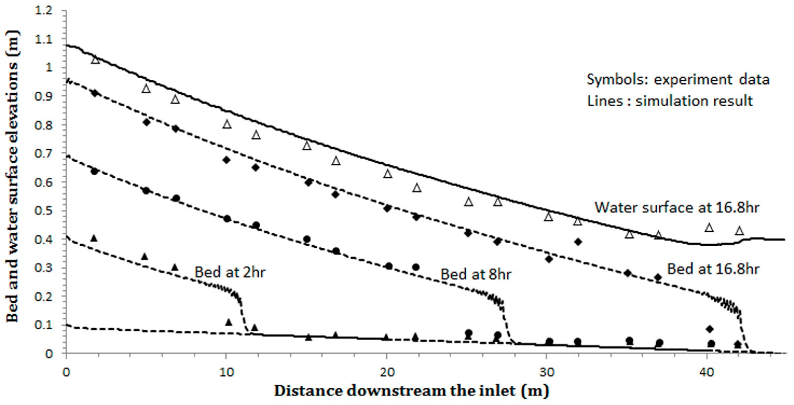
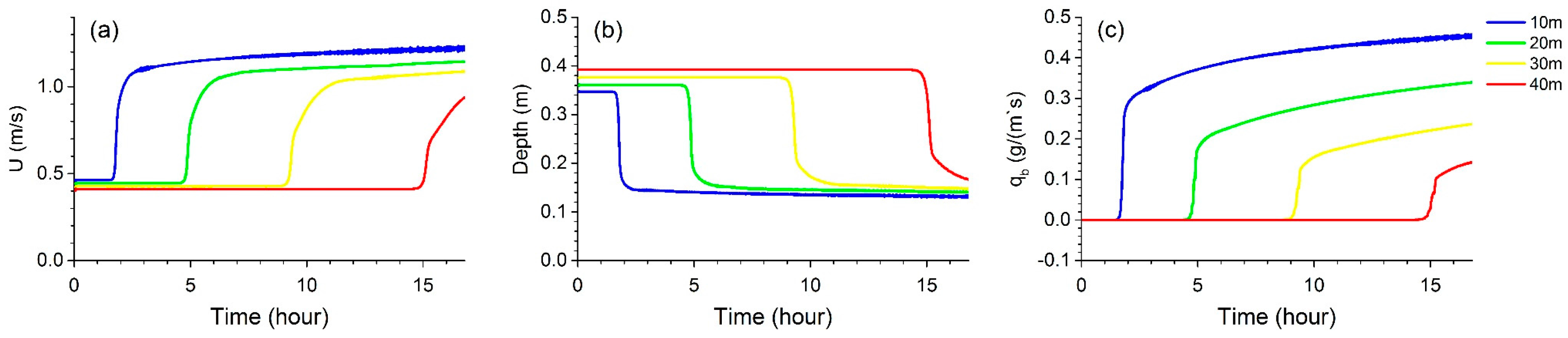
The predicted result together with the experimental data is shown in Figure 1. Generally, the model predicts the bed elevation and the water surface well. As the water and sediment mixture flowed into the channel, sediment particles were deposited onto the bed and caused it to aggrade quickly. The riverbed aggraded vertically with an average speed of 0.0518 m/h, and the downstream head of the newly formed bed moved forward with an average speed of about 2.5 m/h. The aggrading bed was relatively flat with a slope of about 0.2%, which agreed closely with the experimental data. For the longitudinal water surface curve, some oscillations were observed near the upstream inlet when the flow was very shallow, but the oscillations did not develop. The water elevation at 16.8 h was generally simulated well. A hydraulic jump could be observed at the downstream end of the main bed deposit, which was also observed in the experiments. Near the bar, there was a rapid water level change, where the Froude number increased rapidly from 0.2 to 0.9. It illustrates that the hydrodynamic model is capable of coping with sudden hydraulic changes. Figure 2 shows the model-predicted time series of flow velocity, water surface elevation, and bed load transport rate at sequential downstream locations of a 10 m step. It illustrates the variations in local hydraulic conditions as the bed aggrades. Due to a steeper bed slope on the newly formed riverbed, the flow sped up, with a high sediment concentration and a shallower water depth of 0.12 m (compared to the original depth of 0.4 m). Similar changes occurred sequentially along the model river as the newly formed bed grew downstream.
3. Braided River Simulation
3.1. Model Setup
The model was applied to a laboratory experiment conducted by Egozi and Ashmore [31], in which a braided river pattern was generally developed. The river was originally designed to be a generic Froude-scaled model with the prototype being the Sunwapta River in Canada. Froude-scaled models have often been applied in geomorphological studies of gravel braided rivers (e.g., [48,49,50,51]). They satisfy the same Froude number (Fr) as natural rivers yet relax the Reynolds similarity criterion for flows that are hydraulically rough and turbulent. Such a model does not produce exact plan-form similarity for a particular river but yields sampling results applicable to full scale rivers in general [52].
The experiments were performed in an 18 m long and 3 m wide flume, with a constant slope of 0.015. The numerical model was set up by adopting the experimental conditions (Figure 3). The sediments were divided into nine groups, with the size fraction boundaries listed in Table 1. Three bed layers were adopted. Initially the bed was assumed to be flattened, with a trapezoidal straight channel in the middle (Figure 3b). The spatial step was set to 2 cm, while an adaptive time step was used to enhance computational efficiency [35], with the minimum and maximum time steps being 0.001 s and 0.01 s, respectively. The minimum water depth used to resolve the drying and flooding of the floodplain was 1 mm. The model simulation time was approximately 133 h, during which the discharge increased from 1.4 L/s to 2.1 L/s at time t = 71.5 h. The sediments were collected from the outlet and then re-fed to the upstream boundary of inlet, just the same as in the experiment.
3.2. Morphodynamic Properties
3.2.1. River Evolution Processes and Phenomena
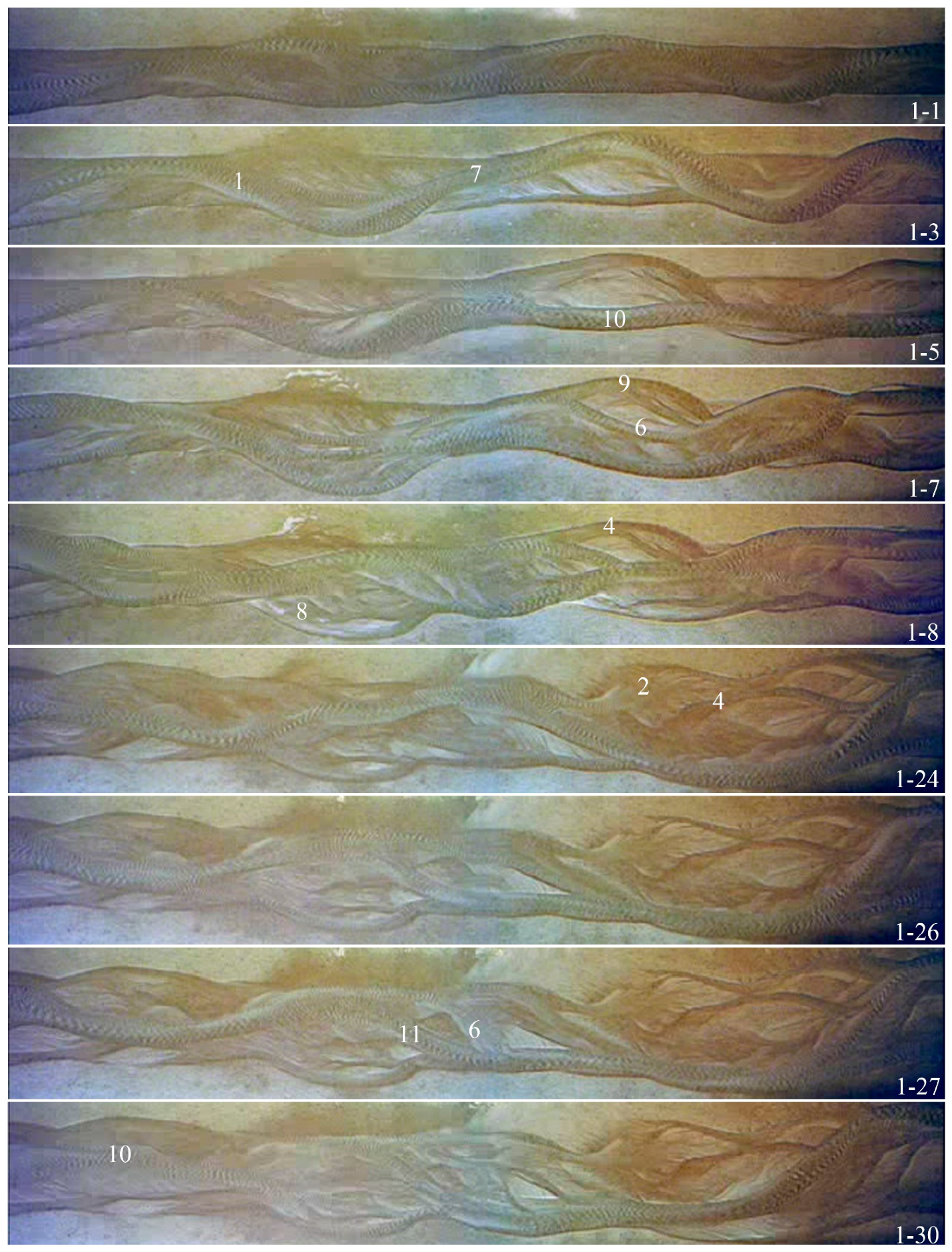
The time serial pictures denoting the evolution process of the model-predicted river are shown in Figure 4. It can be observed that the development of a braided pattern in the predicted river shares many common properties with the experimental river (Figure 5, activity number identified with Figure 4). Most of the morphologic elements and activities observed in the experimental river [31] have been found in the predicted river.
In the first few hours of model simulation, alternate bars and channels were formed in the upstream reach, mainly distributed in the initially cut channel (hour 8). Next, one main channel began to take shape under the strengthening connection of the alternate channels by incision, bank erosion, and channel migration (hour 12). In this channel, the water depth increased further along with increasing sinuosity (hour 19, point 1). Intense erosion occurred along the bank of the initially cut channel, and the channel migrated outward. As the channel became more sinuous, the water overflowed from the banks of certain local bends and spread across the unchannelled margins downstream of the bends (hour 24, point 2), which were called ‘pseudoanabranches’ and sometimes grew into new channels. At certain local bends, the channel was dissected by the upstream tributary, and one bifurcation was formed (hour 24, point 3). At the bifurcation of the newly avulsed areas, the flow rate decreased in the original main channel and increased in the new channel, and the new channel consequently became more dominant, whilst the old channel died out gradually. This activity can be called avulsion by incision [15], through which the main channel tends to find a straighter pathway by incising a new course.
The braiding configuration was developed by hour 27. Some active channels reconnected with each other again by overflow or new channel erosion (hour 27, point 5), while some secondary channels were gradually abandoned (hour 27, point 4). As some channels became more sinuous, water overflowed at the bends, forming new channels (hour 24, point 6). Flow concentrated in the main channel, and accordingly it formed another channel bend (hour 36, point 7). Certain channels were choked by sediment deposition (hour 38, point 8), which can be classified as avulsion by progradation [15]. By hour 40, the upstream reach had widened significantly by extending downstream and into the original margin areas, evolving into a new stage. One of the bifurcated channels captured a large amount of flow from another and finally evolved into a deep channel, followed by the disappearance of the original dominant channel of a bifurcation (hour 44, point 9). The main channel shifted to one of its tributaries as the upstream flow conditions changed (hour 44, point 10). Certain previous abandoned channels (hour 38, point 8) were regenerated by channel annexation (hour 47, point 11). In the predicted river, a cycle of straight channels transitioning to sinuous channels and then to avulsions is an important morphodynamic process during the evolutionary process of the braided river. These activities play an important role in maintaining the dynamic braided form.
3.2.2. Properties of a Typical Braided River
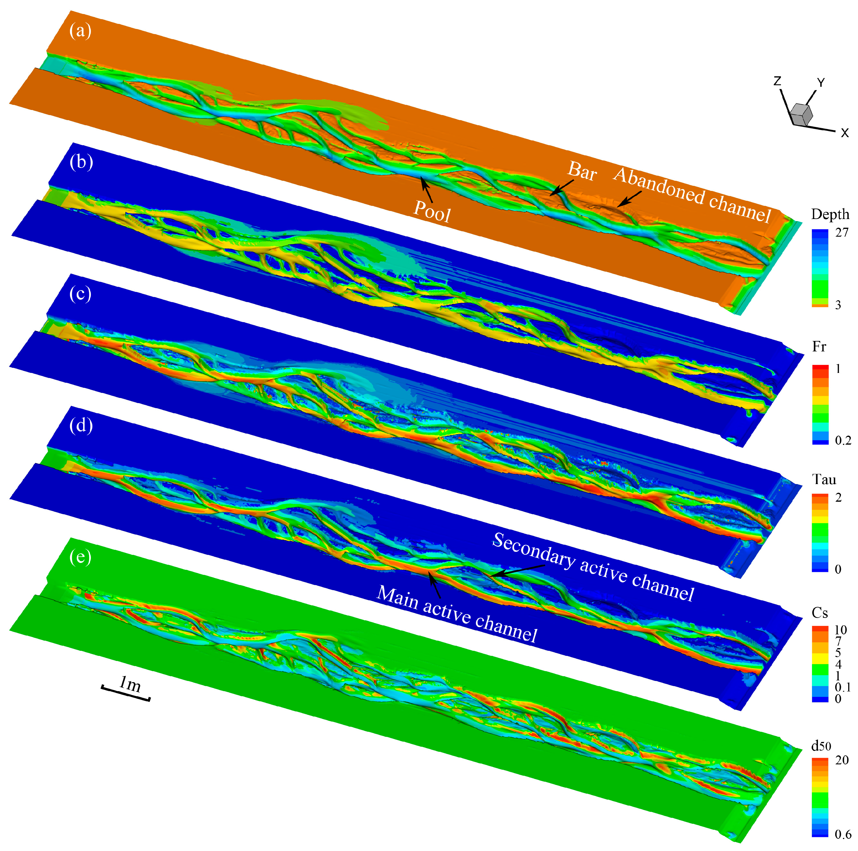
The model riverbed was initially flat with a straight channel in the middle of the flume, and it gradually evolved into a braided river. A typical braided river was generated after 41 h, with the distributions of water depth, Froude number, bed shear stress, bed load concentration, and sediment distribution shown in Figure 6. Key channel nodes, including bars, confluences, bifurcations, and a series of sequential pool-bar units with repeated division and joining of channels can be observed (Figure 6a). These features share many similarities with the experimental river and natural rivers (e.g., [7,31,53]).
For most of the active channels, the Froude number was between 0.6 and 0.7 (Figure 6b). In some local areas, especially in the areas where confluence and bifurcation occurred, the Froude number varied in a range of 0.7 to 1.0. The distribution of bed shear stress has been shown to be relative to bed grain size distribution and water depth (Figure 6c). Higher shear stress values occurred mainly in the main channel and bifurcation areas, and at times they also existed along channel edges.
An active channel is defined as a channel with visible bed material movement [54]. In the simulated river, if the bed load concentration is higher than a certain value (e.g., 6 g/m3), it can be considered ‘active’; otherwise, it is considered ‘non-active’. In that sense, a main active channel formed in the river with the highest sediment concentration, and other active channels joined and bifurcated from it (Figure 6d), which was similar to the experimental river. Due to the special sediment load method in the experiment in which ‘the sand leaving the end of the flume was recirculated from the tail tank and fed back into the flume’ [31], finer sediments were more involved in the circulation because it was easier for them to be transported; therefore, the sediments were often coarser on the two sides of a channel than in the thalweg (Figure 6e).
3.2.3. Sensitivity Analysis
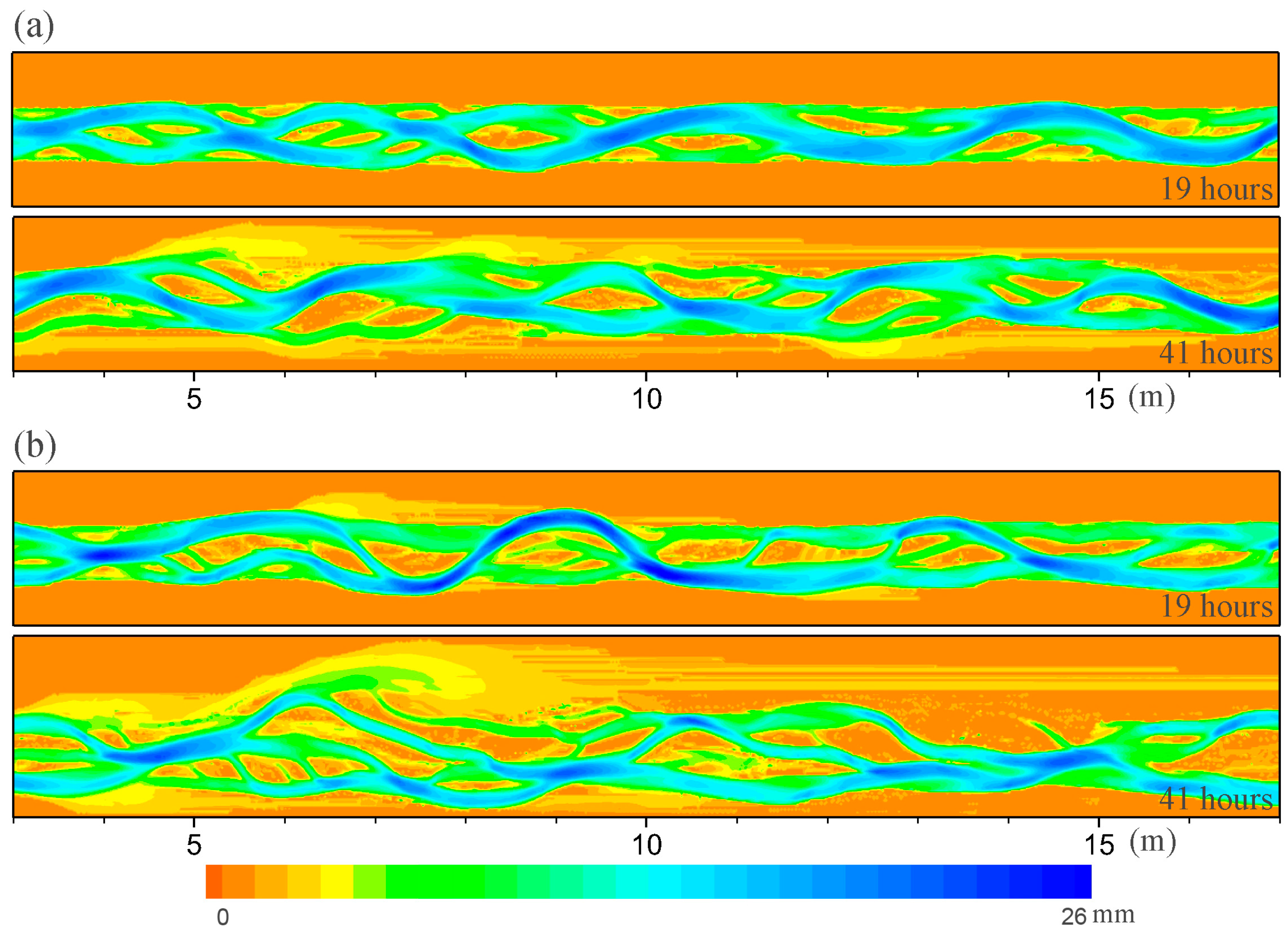
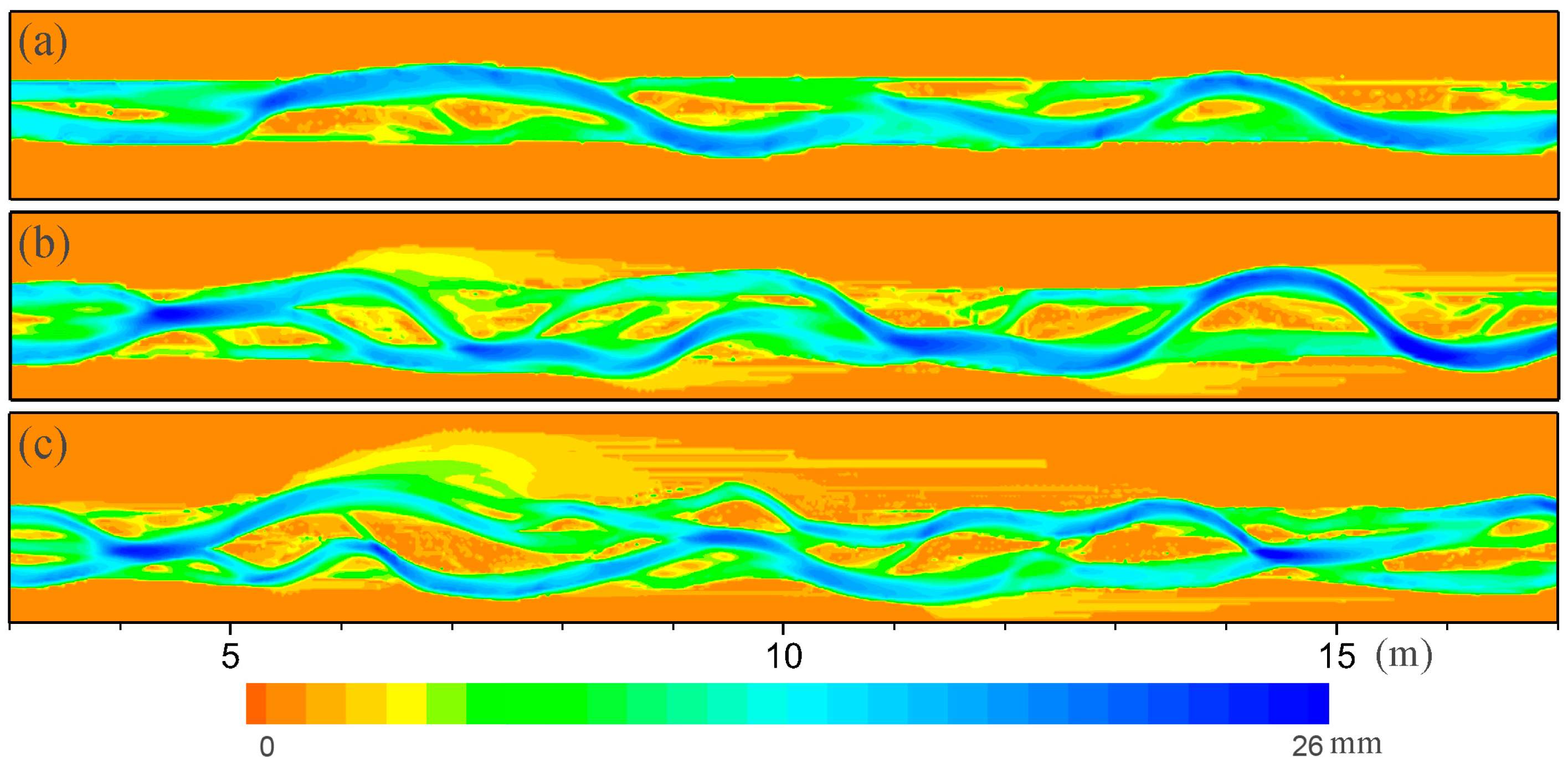
A sensitivity analysis was performed to investigate the effects of secondary flow and grid size on the model performance. Without considering the effect of secondary flow (Figure 7a), a river with alternating pool-bar units also formed, and a braided pattern was generated at hour 41. This river shared a similar channel pattern with the river considering the effect of secondary flow (Figure 7b), yet it generated fewer but wider channels with a slower development rate, illustrating the role that the secondary flow plays in transverse sediment transport and channel migration.
Figure 8 shows the braiding configurations with grids of (a) 0.03 × 0.03 m2, (b) 0.025 × 0.025 m2, and (c) 0.02 × 0.02 m2 at hour 27. Compared with the river with a cell size of 0.02 × 0.02 m2, the river with a lower resolution of 0.03 × 0.03 m2 produced fewer and wider channels. In contrast, the river with a middle cell resolution of 0.025 × 0.025 m2 generated a similar braided pattern to the river with a cell size of 0.02 × 0.02 m2. The channel numbers and widths of these two rivers were comparable with each other.
3.3. Statistical Characteristics
Due to the nature of braided rivers with frequent channel migrations, statistical methods are usually employed to assess the characteristics of braided rivers [55]. Given that braided rivers in nature exhibit some intrinsic characteristics common to all braided rivers, several methods have been proposed to evaluate the simulation capability of physical and numerical models (e.g., [55,56]). In the present study, three statistical methods, including braiding intensity, state-space plots, and transect topography and slope frequency, were applied to evaluate the model-predicted river.
3.3.1. Braiding Intensity
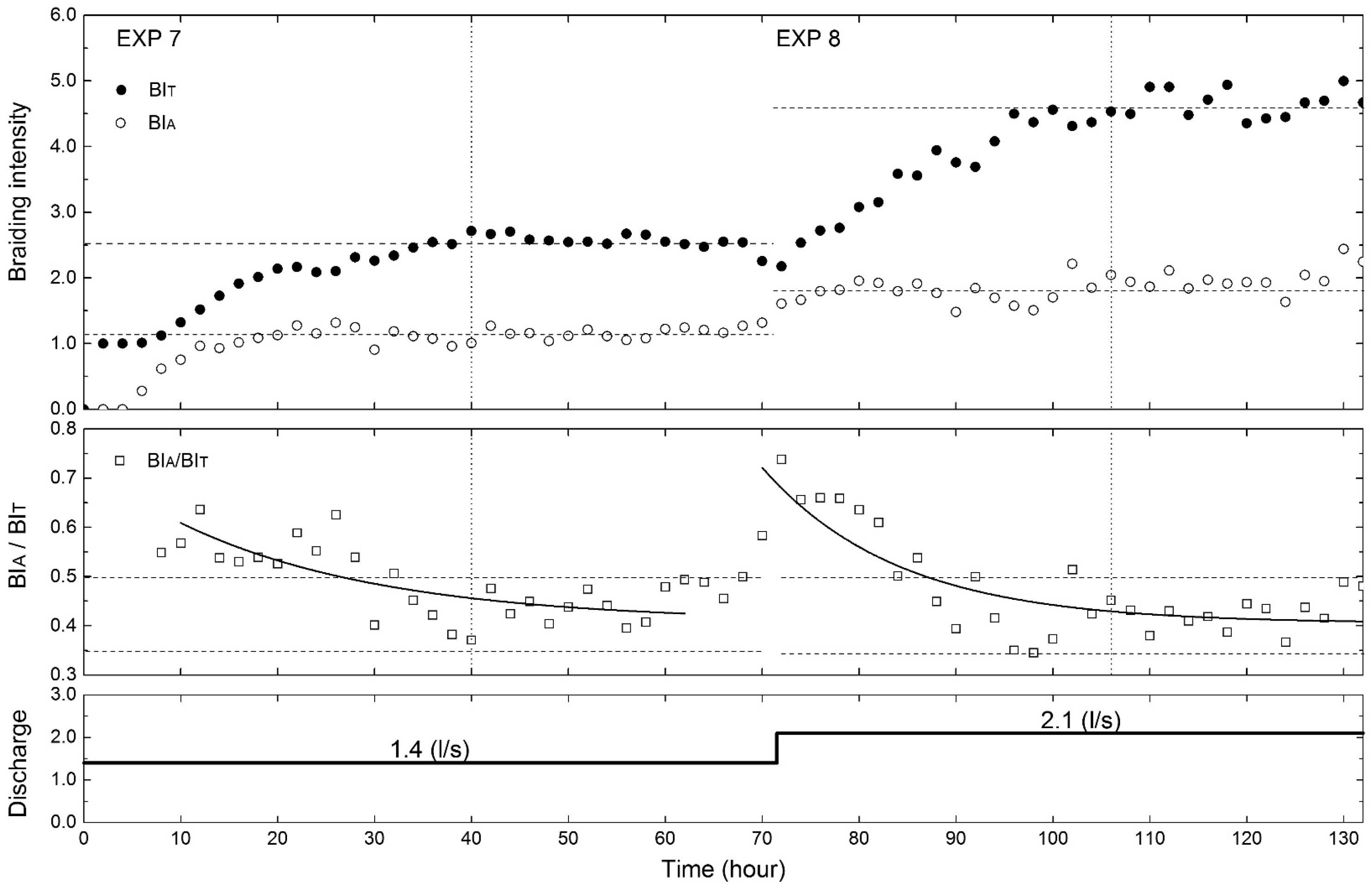
Braiding intensity has been proposed to measure the channel intensity in braided rivers [54,57,58]. Total braiding intensity (BIT) (defined as the number of total wetted channels counted and averaged over a number of cross sections of a river), active braiding intensity (BIA) (defined as the number of channels with visible bed load sediment transport counted and averaged over a number of cross sections of a river), and their ratio (BIT/BIA) were calculated (Figure 9) and compared with the experimental results (Table 2). In general, the model successfully predicted the response of the channel pattern to increasing discharge, with the total and active braiding intensities increased to new stages. The maximum BIT values were greater than twice the maximum BIA values, which were similar to those observed in the experiments [31]. Compared with the experimental river, the model-predicted river developed nearly the same BIA and a slightly lower BIT in Experiment 7. However, in Experiment 8, the differences between the model-predicted and the measured BIA and BIT values increased after hour 100. This is because several channels co-existed and the difference between the main channel and other channels became less obvious.
In both flow stages, the active braiding intensity, BIA, developed quickly to a stable value (Figure 9). In the first stage, it took slightly longer to stabilize, but, in the second stage, it took only a couple of hours. In contrast, BIT took a much longer time to increase progressively to a stable state (approximately 40 h). The quick stabilization of BIA was explained by Egozi and Ashmore [31] as follows: the increase in BIA requires only a sufficiently large flow within an existing channel to mobilize the bed material, and this can be accomplished very quickly; however, the increase in BIT needs time for the river to erode new channels, resulting in a much longer time for its stabilization. The longer duration for the stabilization of BIA and BIT during the first flow stage resulted from the fact that it took some time to develop a braided pattern from the initially straight channel. The variation in BIA/BIT shows a consistent trend progressively approaching nearly 0.4 (Figure 9), which shared similar stable values of BIA / BIT with the experimental river but with a slightly narrower range (Table 2).
3.3.2. State Space Plots
Natural braided rivers have shown an intertwining effect of braiding, represented by the repeated division and joining of channels with bars between them [7]. Flow at one location affects the downstream morphology, and braided rivers show recurring geometric and topographic characteristics. A method named ‘state-space plot’ has been employed to evaluate the spatial recurring patterns of braided rivers (e.g., [56]). The state-space plot is constructed using a series of values of one essential variable by plotting each value versus the previous value at its neighbouring upstream cross section, and when it moves from one point to the successive points and eventually forms a closed loop, the information on spatial order is recorded. The total channel widths, sequential scour depths at channel confluences, and heights of successive bars have been proposed to analyse the spatial repeating pattern of braided rivers [21,55,59,60].
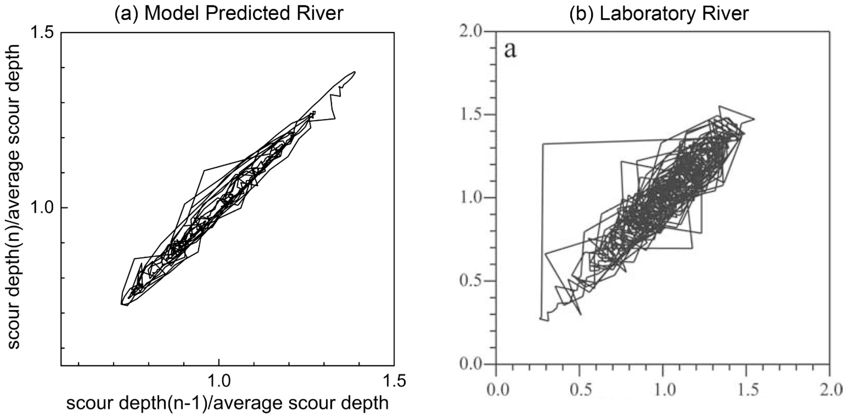
In the present study, the maximum scour depth in each cross-section was chosen for state-space plotting. With the data of a fully developed braided river, state-space plots were constructed by plotting the scour depth versus the preceding scour depth, both normalised to the overall scour depth. Figure 10 shows the state space plots of the predicted river and a laboratory river [60]. Clusters of loops can be seen in the plots of the predicted river and the laboratory river, indicating that they share a common statistically spatial repeating pattern. However, the predicted river has a thinner pattern than the laboratory river, indicating that, in the laboratory river, the channel scour depth changes in a more abrupt way than in the predicted river. Nonetheless, crossing lines were more common for the laboratory river than for the predicted river. They were considered to originate from some statistic behaviour of the rivers [59].
3.3.3. Transect Topography and Slope Frequency
The riverbed topography structure can be described by cross-section surveys such as the transect topography and the cumulative frequency of lateral slopes [55]. The former provides direct transect distributions of bed topographic highs and lows. The latter estimates the frequency of bed lateral slopes relative to a reference level; for example, the median elevation. They can be employed to assess the similarities between the simulated and natural rivers.
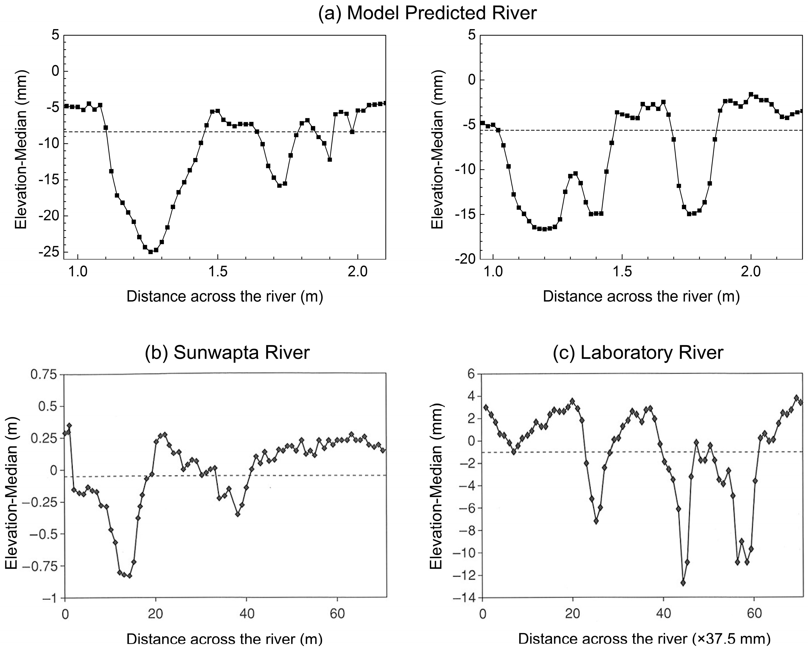
The predicted river with a fully developed braided pattern was analysed to determine the structure of the transect topography. The results of two representative cross-sections are shown in Figure 11, together with those from the Sunwapta River and a laboratory river [55], with the Sunwapta River being the prototype of the experimental river simulated in the present study. It can be seen that, in the cross-sections shown in Figure 11, the channels are relatively narrow and deep, while the bars are relatively wide and gentle, with the maximum scour depth of the channels exceeding the maximum deposition height of the bars. These are common characteristics for the model-predicted river and the prototype natural and laboratory rivers. However, compared to the Sunwapta River and laboratory river, the predicted river presents a smoother cross-sectional bed elevation. This indicates that the riverbed of the simulated river is more ideal than those of real rivers.
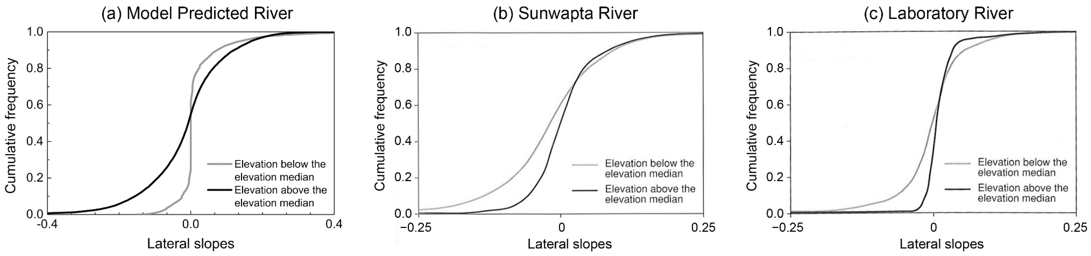
The slope frequency distribution curves were constructed based on the cross-section slopes in the model predicted reach of 4 to 17 m, containing the data of 650 cross-sections. Figure 12 shows the results of the predicted river at hour 41, the Sunwapta River, and a laboratory river [55], all of which present similar varying trends. The curves corresponding to the channels are significantly wider than the bars, illustrating that the bars exhibit statistically gentler elevation changes than do the channels. This is consistent with the findings from the bed-transect topographic distributions (Figure 11). The steep sides in the channels were produced by fast flow and energetic erosion activity, while an opposite situation occurred on the bars. In addition, the wider slope frequency domains of both the channels and the bars for the predicted river indicate that statistically the predicted river channels are slightly steeper than those of the Sunwapta River and the laboratory river.
4. Discussion and Conclusions
A physics-based numerical model was developed to simulate the morphodynamic processes in laboratory braided rivers with non-uniform bed load transport. The model applied the basic hydrodynamic and sediment transport principles with a fractional method and multiple bed layers. It employed the TVD-MacCormack Scheme for solving the hydrodynamic equations of trans-critical flows, and was tested with a sediment aggradation case and found to be capable of effectively predicting the flow and bed deformation.
With the same boundary conditions as an experimental river, the model successfully reproduced the evolution processes and phenomena of braiding, avulsion activities, and the responses of the channel pattern to increased discharge. The incorporation of the effect of secondary flow played an essential role in producing a more realistic braided pattern. Certain geomorphologic phenomena and processes observed in the experimental river and natural rivers have been found in the evolutionary process of the predicted river. A cycle of straight channels transitioning to sinuous channels and then to avulsions was an important morphodynamic process for the river to maintain a dynamic braided form. Avulsion activities with similar evolution processes to natural rivers have been found in both the experimental and predicted rivers. A high shear stress usually occurred in areas where the flow was energetic, erosion was possible, and the riverbed sediment was mainly composed of coarse bed material. The changes in the braiding intensities illustrated trends similar to those in the experimental river in the process of braiding generation and in response to increased discharge. Active braiding intensity developed quickly to a stable value, whereas total braiding intensity increased to a stable state gradually due to the time consumed by cutting new channels. The predicted river shared common statistical topographic characteristics with natural and laboratory rivers, showing a recurring spatial pattern of shallow and deep topography and statistical transect gentle bars and steep channels.
Generally, the results presented above demonstrate the potential for the present model to represent the morphodynamic processes of natural braided rivers. Nevertheless, it is necessary to gradually improve the understanding and capability of the model in conjunction with field research and laboratory experiments.
Acknowledgments
We are grateful for the financial support from the State Key Laboratory of Hydroscience and Engineering, Tsinghua University (2015-ky-2), the Guangzhou Science Technology and Innovation Commission (201605030009), and the South China Agricultural University (7600-217244). We thank Roey Egozi and Ana Maria A.F. da Silva for their comments and suggestions on the present research.
Author Contributions
Haiyan Yang and Binliang Lin conceived of the braided river simulation research and developed the physics-based model; Haiyan, Jian Sun and Guoxian Huang set up and debugged the programmes; Haiyan Yang analysed the results and wrote the paper; Haiyan Yang and Binliang Lin provided editorial improvements to the paper.
Conflicts of Interest
The authors declare no conflicts of interest. The founding sponsors had no role in the design of the study; in the collection, analyses, or interpretation of data; in the writing of the manuscript; nor in the decision to publish the results.
References
- Bertoldi, W.; Gurnell, A.; Surian, N.; Tockner, K.; Zanoni, L.; Ziliani, L.; Zolezzi, G. Understanding reference processes: Linkages between river flows, sediment dynamics and vegetated landforms along the Tagliamento River, Italy. River Res. Appl. 2009, 25, 501–516. [Google Scholar] [CrossRef]
- Knighton, D.A. Fluvial Forms and Processes: A New Perspective; Arnold, Hodder Headline, PLC: London, UK, 1998; p. 383. [Google Scholar]
- Ham, D.G.; Church, M. Bed-material transport estimated from channel morphodynamics: Chilliwack River, British Columbia. Earth Surf. Process. Landf. 2000, 25, 1123–1142. [Google Scholar] [CrossRef]
- Smith, N.D.; Smith, D.G. William River: An outstanding example of channel widening and braiding caused by bed-load addition. Geology 1984, 12, 78. [Google Scholar] [CrossRef]
- Brierley, G.J.; Hickin, E.J. Channel planform as a non-controlling factor in fluvial sedimentology: The case of the Squamish River floodplain, British Columbia. Sediment. Geol. 1991, 75, 67–83. [Google Scholar] [CrossRef]
- Huang, H.Q.; Chang, H.H.; Nanson, G.C. Minimum energy as the general form of critical flow and maximum flow efficiency and for explaining variations in river channel pattern. Water Resour. Res. 2004, 40, W04502. [Google Scholar] [CrossRef]
- Bridge, J.S. The interaction between channel geometry, water flow, sediment transport and deposition in braided rivers. In Braided Rivers; Best, J.L., Bristow, C.S., Eds.; Geological Society: London, UK, 1993; pp. 13–71. [Google Scholar]
- Cui, Y.; Paola, C.; Parker, G. Numerical simulation of aggradation and downstream fining. J. Hydraul. Res. 1996, 34, 185–204. [Google Scholar] [CrossRef]
- Duc, B.M.; Wenka, T.; Rodi, W. Numerical modeling of bed deformation in laboratory channels. J. Hydraul. Eng. 2004, 130, 894–904. [Google Scholar] [CrossRef]
- Meselhe, E.A.; Georgiou, I.; Allison, M.A.; McCorquodale, J.A. Numerical modeling of hydrodynamics and sediment transport in lower Mississippi at a proposed delta building diversion. J. Hydrol. 2012, 472, 340–354. [Google Scholar] [CrossRef]
- Bai, Y.; Duan, J.G. Simulating unsteady flow and sediment transport in vegetated channel network. J. Hydrol. 2014, 515, 90–102. [Google Scholar] [CrossRef]
- Murray, A.B.; Paola, C. A cellular model of braided rivers. Nature 1994, 371, 54–57. [Google Scholar] [CrossRef]
- Coulthard, T.J.; Hicks, D.M.; Van De Wiel, M.J. Cellular modelling of river catchments and reaches: Advantages, limitations and prospects. Geomorphology 2007, 90, 192–207. [Google Scholar] [CrossRef]
- Schuurman, F.; Marra, W.A.; Kleinhans, M.G. Physics-based modeling of large braided sand-bed rivers: Bar pattern formation, dynamics, and sensitivity. J. Geophys. Res. 2013, 118, 2509–2527. [Google Scholar] [CrossRef]
- Slingerland, R.; Smith, N.D. River avulsions and their deposits. Annu. Rev. Earth Planet. Sci. 2004, 32, 257–285. [Google Scholar] [CrossRef]
- Jang, C.L.; Shimizu, Y. Numerical simulations of the behavior of alternate bars with different bank strengths. J. Hydraul. Res. 2005, 43, 596–612. [Google Scholar] [CrossRef]
- Jang, C.L.; Shimizu, Y. Numerical simulation of relatively wide, shallow channels with erodible banks. J. Hydraul. Eng. 2005, 131, 565–575. [Google Scholar] [CrossRef]
- Nicholas, A.P. Modelling the continuum of river channel patterns. Earth Surf. Process. Landf. 2013, 38, 1187–1196. [Google Scholar] [CrossRef]
- Schuurman, F.; Kleinhans, M.G. Bar dynamics and bifurcation evolution in a modelled braided sand-bed river. Earth Surf. Process. Landf. 2015, 40, 1318–1333. [Google Scholar] [CrossRef]
- Yang, H. Development of a Physics-Based Morphodynamic Model and Its Application to Braided Rivers. Ph.D. Thesis, Cardiff University, Cardiff, UK, 2013. [Google Scholar]
- Yang, H.; Lin, B.; Zhou, J. Physics-based numerical modelling of large braided rivers dominated by suspended sediment. Hydrol. Process. 2015, 29, 1925–1941. [Google Scholar] [CrossRef]
- Kleinhans, M.G. Sorting out river channel patterns. Prog. Phys. Geogr. 2010, 34, 287–326. [Google Scholar] [CrossRef]
- Takebayashi, H.; Okabe, T. Numerical modelling of braided streams in unsteady flow. Proc. ICE Water Manag. 2009, 162, 189–198. [Google Scholar] [CrossRef]
- Lotsari, E.; Wainwright, D.; Corner, G.D.; Alho, P.; Kayhko, J. Surveyed and modelled one-year morphodynamics in the braided lower Tana River. Hydrol. Process. 2014, 28, 2685–2716. [Google Scholar] [CrossRef]
- Schuurman, F.; Kleinhans, M.G. Self-Formed Braid Bars in a Numerical Model; American Geophysical Union Fall Meeting Abstracts: Washington, DC, USA, 2011; p. 672. [Google Scholar]
- Ikeda, S.; Parker, G.; Sawai, K. Bend theory of river meanders, part 1: Linear development. J. Fluid Mech. 1981, 112, 363–377. [Google Scholar] [CrossRef]
- Parker, G.; Sawai, K.; Ikeda, S. Bend theory of river meanders, part 2: Nonlinear deformation of Finite-amplitude bends. J. Fluid Mech. 1982, 115, 303–314. [Google Scholar] [CrossRef]
- Kleinhans, M.G.; van den Berg, J.H. River channel and bar patterns explained and predicted by an empirical and a physics-based method. Earth Surf. Process. Landf. 2011, 36, 721–738. [Google Scholar] [CrossRef]
- Wu, W. Computational River Dynamics; Taylor & Francis Group: London, UK, 2007; p. 499. [Google Scholar]
- Ferguson, R.I.; Ashmore, P.E.; Ashworth, P.J.; Paola, C.; Prestegaard, K.L. Measurements in a braided river chute and lobe: 1. Flow pattern, sediment transport, and channel change. Water Resour. Res. 1992, 28, 1877–1886. [Google Scholar] [CrossRef]
- Egozi, R.; Ashmore, P.E. Experimental analysis of braided channel pattern response to increased discharge. J. Geophys. Res. 2009, 114. [Google Scholar] [CrossRef]
- Leduc, P.; Ashmore, P.; Gardner, J.T. Grain sorting in the morphological active layer of a braided river physical model. Earth Surf. Dyn. 2015, 3, 577. [Google Scholar]
- Van Niekerk, A.; Vogel, K.R.; Slingerland, R.L.; Bridge, J.S. Routing of heterogeneous sediments over movable bed: Model development. J. Hydraul. Eng. 1992, 118, 246–262. [Google Scholar] [CrossRef]
- Van Rijn, L.C. Sediment transport, part III: Bed forms and alluvial roughness. J. Hydraul. Eng. 1984, 110, 1733–1754. [Google Scholar] [CrossRef]
- Liang, D.; Falconer, R.A.; Lin, B. Comparison between TVD-MacCormack and ADI-type solvers of the shallow water equations. Adv. Water Resour. 2006, 29, 1833–1845. [Google Scholar] [CrossRef]
- Liang, D.; Lin, B.; Falconer, R.A. Simulation of rapidly varying flow using an efficient TVD-MacCormack scheme. Int. J. Numer. Methods Fluids 2007, 53, 811–826. [Google Scholar] [CrossRef]
- Van Rijn, L.C. Sediment transport, part I: Bed load transport. J. Hydraul. Eng. 1984, 110, 1431–1456. [Google Scholar] [CrossRef]
- Van Rijn, L.C. Principles of Sediment Transport in Rivers, Estuaries and Coastal Seas; Aqua Publications: Amsterdam, The Netherlands, 1993. [Google Scholar]
- Engelund, F. Flow and bed topography in channel bends. J. Hydraul. Div 1974, 100, 1631–1648. [Google Scholar]
- Karim, F. Bed material discharge prediction for nonuniform bed sediments. J. Hydraul. Eng. 1998, 124, 597–604. [Google Scholar] [CrossRef]
- Van Rijn, L.C. Unified view of sediment transport by currents and waves III: Graded beds. J. Hydraul. Eng. 2007, 133, 761–775. [Google Scholar] [CrossRef]
- Wei, Z.L. One Dimensional Sediment Model for the Yellow River; Report of Wuhan University of Hydro-electrical Power (In Chinese). Wuhan University: Wuhan, China, 1993. [Google Scholar]
- Zhou, J.; Lin, B. Modelling Bed Evolution Processes in Alluvial Rivers. In Proceedings of the International Conference on Fluvial Hydraulics, Izmir, Turkey, 3–5 September 2008; pp. 1305–1311. [Google Scholar]
- Lin, B.; Falconer, R.A. Tidal flow and transport modeling using Ultimate Quickest scheme. J. Hydraul. Eng. 1997, 123, 303–314. [Google Scholar] [CrossRef]
- Sun, J.; Lin, B.; Yang, H. Development and application of a braided river model with non-uniform sediment transport. Adv. Water Resour. 2015, 81, 62–74. [Google Scholar] [CrossRef]
- Seal, R.; Paola, C.; Parker, G.; Southard, J.B.; Wilcock, P.R. Experiments on downstream fining of gravel: I. Narrow-channel runs. J. Hydraul. Eng. 1997, 123, 874–884. [Google Scholar] [CrossRef]
- Paola, C.; Parker, G.; Seal, R.; Sinha, S.K.; Southard, J.B.; Wilcock, P.R. Downstream fining by selective deposition in a laboratory flume. Science 1992, 258, 1757–1760. [Google Scholar] [CrossRef] [PubMed]
- Ashmore, P.E. Channel morphology and bed load pulses in braided, gravel-bed streams. Geogr. Ann. Ser. A 1991, 73, 37–52. [Google Scholar] [CrossRef]
- Hoey, T.; Sutherland, A.J. Channel morphology and bedload pulses in braided rivers: A laboratory study. Earth Surf. Process. Landf. 1991, 16, 447–462. [Google Scholar] [CrossRef]
- Shvidchenko, A.B.; Kopaliani, Z.D. Hydraulic modeling bed load transport in gravel bed Laba River. J. Hydraul. Eng. 1998, 124, 778–785. [Google Scholar] [CrossRef]
- Warburton, J.; Davies, T.R.H. Use of hydraulic models in management of braided gravel-bed rivers. In Gravel-Bed Rivers in the Environment; Klingeman, P.C., Beschta, R.L., Komar, P.D., Bradley, J.B., Eds.; Water Resources Publications: Littleton, CO, USA, 1998; pp. 512–542. [Google Scholar]
- Egozi, R.; Ashmore, P.E. Defining and measuring braiding intensity. Earth Surf. Process. Landf. 2008, 33, 2121–2138. [Google Scholar] [CrossRef]
- Ashmore, P.E. Anabranch confluence kinetics and sedimentation processes in gravel-braided streams. In Braided Rivers; Best, J.L., Bristow, C.S., Eds.; Geological Society, Special Publications: London, UK, 1993; Volume 75, pp. 129–146. [Google Scholar]
- Ashmore, P.; Bertoldi, W.; Tobias Gardner, J. Active width of gravel-bed braided rivers. Earth Surf. Process. Landf. 2011, 36, 1510–1521. [Google Scholar] [CrossRef]
- Doeschl, A.B.; Ashmore, P.E.; Davison, M. Methods for Assessing Exploratory Computational Models of Braided Rivers. In Braided Rivers: Process, Deposits, Ecology and Management; Sambrook-Smith, G.H., Best, J.L., Bristow, C.S., Petts, G.E., Jarvis, I., Eds.; Wiley-Blackwell: Malden, MA, USA, 2006; pp. 177–197. [Google Scholar]
- Murray, A.B.; Paola, C. A new quantitative test of geomorphic models, applied to a model of braided streams. Water Resour. Res. 1996, 32, 2579–2587. [Google Scholar] [CrossRef]
- Ashmore, P.E. How do gravel-bed rivers braid? Can. J. Earth Sci. 1991, 28, 326–341. [Google Scholar] [CrossRef]
- Bertoldi, W.; Zanoni, L.; Tubino, M. Planform dynamics of braided streams. Earth Surf. Process. Landf. 2009, 34, 547–557. [Google Scholar] [CrossRef]
- Sapozhnikov, V.B.; Murray, A.B.; Paola, C.; Foufoula-Georgiou, E. Validation of Braided-Stream Models: Spatial state-space plots, self-affine scaling, and island shapes. Water Resour. Res. 1998, 34, 2353–2364. [Google Scholar] [CrossRef]
- Rosatti, G. Validation of the physical modeling approach for braided rivers. Water Resour. Res. 2002, 38, 1295. [Google Scholar] [CrossRef]
Figure 1.
Predicted bed elevations and water surface of the experiment of Seal et al. [46].
Figure 1.
Predicted bed elevations and water surface of the experiment of Seal et al. [46].

Figure 2.
Model predicted (a) flow velocity; (b) water depth; and (c) bed load transport rate.

Figure 3.
Schematic diagrams of the river flume: (a) schematic flume; (b) horizontal plan; and (c) cross-section A–A’.
Figure 3.
Schematic diagrams of the river flume: (a) schematic flume; (b) horizontal plan; and (c) cross-section A–A’.
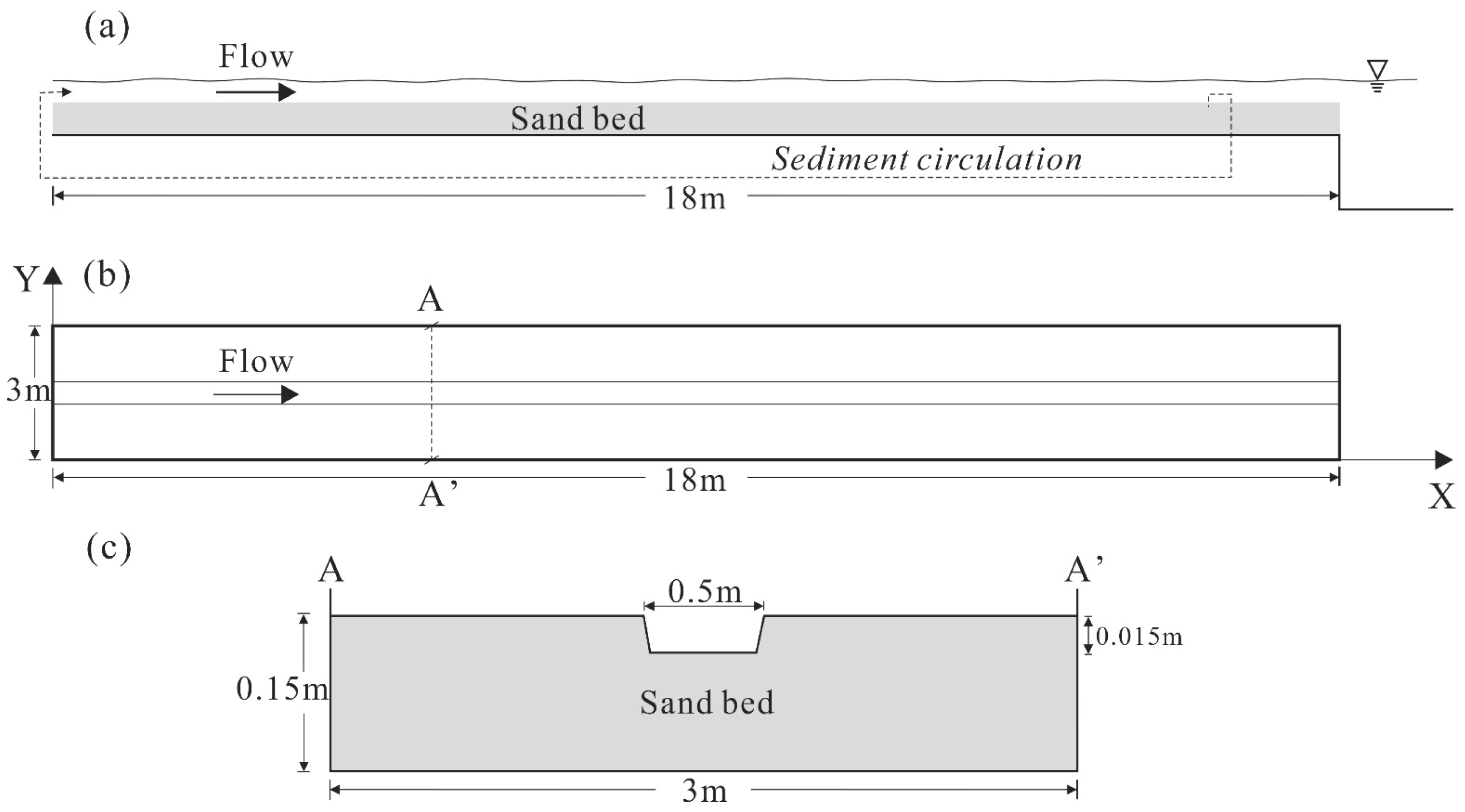
Figure 4.
Morphologic changes and activities during the evolution process of the model predicted river (water depth/mm). 1: increasing sinuosity of the main channel; 2: the generation and obliteration of pseudo-anabranches; 3: avulsion by incision; 4: abandonment of the secondary channel; 5: reconnecting of two active channels; 6: avulsion by overflow; 7: concentration of the flow in the main channel; 8: avulsion by progradation; 9: water diversion from one secondary channel to an existing or new channel; 10: shifting of the main channel; and 11: regeneration of an abandoned channel.
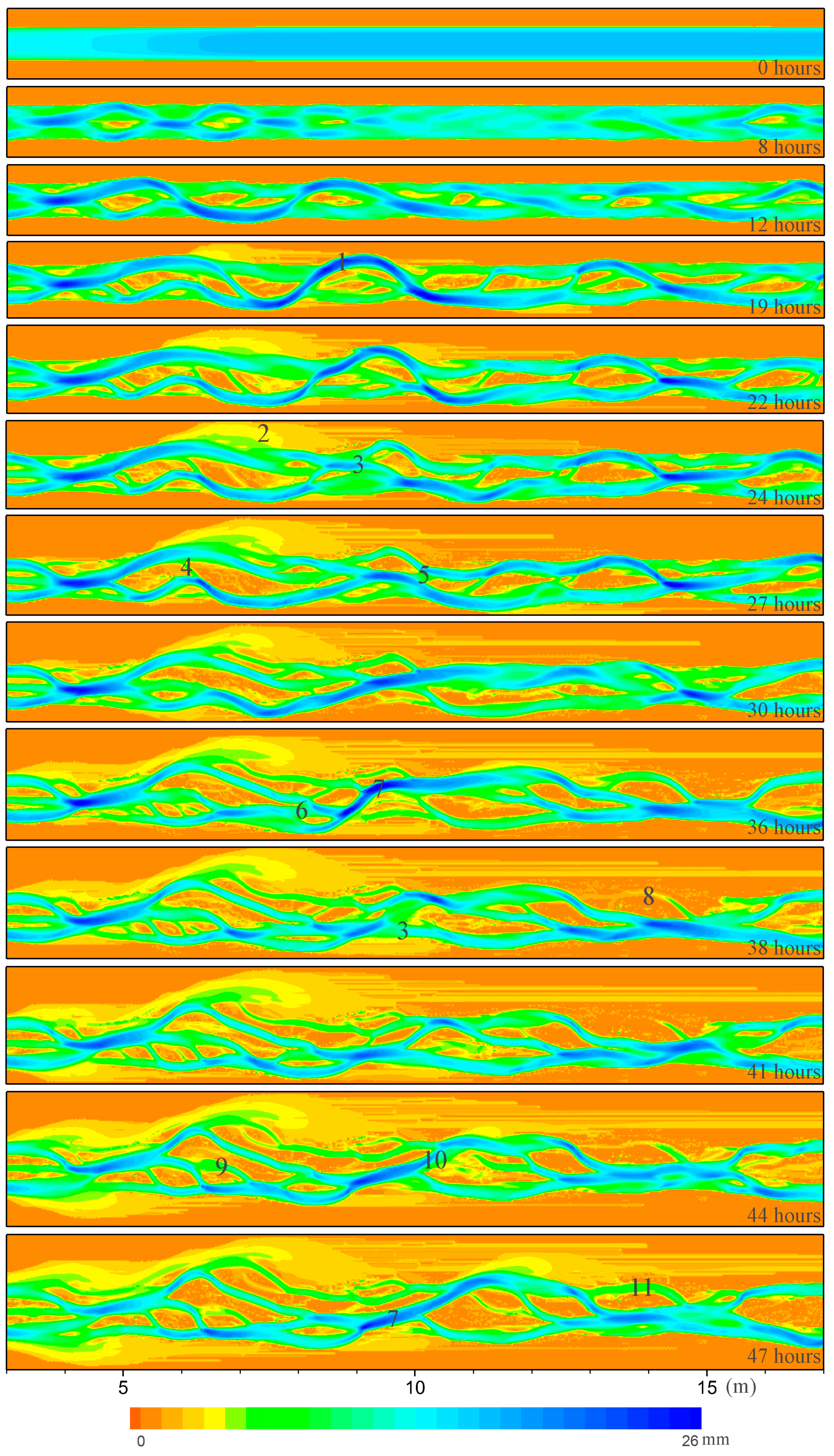
Figure 5.
Morphologic changes and activities during the evolution process of the experimental river with the activity numbers identical to those in Figure 4.
Figure 5.
Morphologic changes and activities during the evolution process of the experimental river with the activity numbers identical to those in Figure 4.

Figure 6.
3-D images of the model predicted river at hour 41: (a) water depth (mm); (b) Froude number; (c) bed shear stress (N/m2); (d) bed load concentration (g/(m·s)); and (e) bed median grain size (mm).
Figure 6.
3-D images of the model predicted river at hour 41: (a) water depth (mm); (b) Froude number; (c) bed shear stress (N/m2); (d) bed load concentration (g/(m·s)); and (e) bed median grain size (mm).

Figure 7.
Braiding configurations (a) without and (b) with the effect of secondary flow.

Figure 8.
Braiding configurations at hour 27 with cell sizes of (a) 0.03 × 0.03 m2; (b) 0.025 × 0.025 m2; and (c) 0.02 × 0.02 m2.
Figure 8.
Braiding configurations at hour 27 with cell sizes of (a) 0.03 × 0.03 m2; (b) 0.025 × 0.025 m2; and (c) 0.02 × 0.02 m2.

Figure 9.
Variations in total braiding intensity (BIT), active braiding intensity (BIA), and BIA/BIT during sequential flow stages.
Figure 9.
Variations in total braiding intensity (BIT), active braiding intensity (BIA), and BIA/BIT during sequential flow stages.

Figure 10.
State-space plots for (a) the model-predicted river and (b) a laboratory river.

Figure 11.
Deviations from the elevation median of cross-sections for (a) the model predicted river; (b) the Sunwapta River; and (c) a laboratory river. The dotted line represents the elevation median.
Figure 11.
Deviations from the elevation median of cross-sections for (a) the model predicted river; (b) the Sunwapta River; and (c) a laboratory river. The dotted line represents the elevation median.

Figure 12.
Cumulative distributions of the lateral slopes of the bars and channels for (a) the model predicted river; (b) the Sunwapta River; and (c) a laboratory river.
Figure 12.
Cumulative distributions of the lateral slopes of the bars and channels for (a) the model predicted river; (b) the Sunwapta River; and (c) a laboratory river.

Table 1.
Sediment fractions in the experimental river and the numerical model.
| Sand Groups | 1 | 2 | 3 | 4 | 5 | 6 | 7 | 8 | 9 | |||||||||
|---|---|---|---|---|---|---|---|---|---|---|---|---|---|---|---|---|---|---|
| Grain Size (mm) | 0.25 | 0.5 | 0.7 | 1.0 | 1.5 | 2.0 | 3.0 | 4.0 | 6.0 | 8.0 | ||||||||
| Percentage (%) | 4.95 | 14.05 | 9.20 | 16.16 | 13.64 | 12.00 | 11.78 | 11.22 | 4.42 | 2.58 | ||||||||
| Finer than (%) | 4.95 | 19.00 | 28.20 | 44.36 | 58.00 | 70.00 | 81.78 | 93.00 | 97.42 | 100.0 | ||||||||
Table 2.
The braiding intensities of the model predicted river and the experimental river.
| Parameters | Predicted River | Experimental River | ||||
|---|---|---|---|---|---|---|
| BIA | BIT | BIA/BIT | BIA | BIT | BIA/BIT | |
| Exp. 7 | 1.1 | 2.6 | 0.35–0.5 | 1.1 | 2.8 | 0.3–0.5 |
| Exp. 8 | 1.8 | 4.5 | 0.35–0.5 | 1.3 | 3.8 | 0.3–0.5 |
© 2017 by the authors. Licensee MDPI, Basel, Switzerland. This article is an open access article distributed under the terms and conditions of the Creative Commons Attribution (CC BY) license (http://creativecommons.org/licenses/by/4.0/).
Share and Cite
MDPI and ACS Style
Yang, H.; Lin, B.; Sun, J.; Huang, G. Simulating Laboratory Braided Rivers with Bed-Load Sediment Transport. Water 2017, 9, 686. https://doi.org/10.3390/w9090686
AMA Style
Yang H, Lin B, Sun J, Huang G. Simulating Laboratory Braided Rivers with Bed-Load Sediment Transport. Water. 2017; 9(9):686. https://doi.org/10.3390/w9090686
Chicago/Turabian StyleYang, Haiyan, Binliang Lin, Jian Sun, and Guoxian Huang. 2017. "Simulating Laboratory Braided Rivers with Bed-Load Sediment Transport" Water 9, no. 9: 686. https://doi.org/10.3390/w9090686
Note that from the first issue of 2016, this journal uses article numbers instead of page numbers. See further details here.