On the Influence of Input Data Quality to Flood Damage Estimation: The Performance of the INSYDE Model


1
Dipartimento di Ingegneria Civile e Ambientale, Politecnico di Milano, 20133 Milano, Italy
2
Dipartimento di Ingegneria Civile, Edile-Architettura e Ambientale, Università degli Studi dell’Aquila, 67100 L’Aquila, Italy
*
Author to whom correspondence should be addressed.
Water 2017, 9(9), 688; https://doi.org/10.3390/w9090688
Submission received: 18 July 2017
/
Revised: 21 August 2017
/
Accepted: 5 September 2017
/
Published: 8 September 2017
Abstract
:IN-depth SYnthetic Model for Flood Damage Estimation (INSYDE) is a model for the estimation of flood damage to residential buildings at the micro-scale. This study investigates the sensitivity of INSYDE to the accuracy of input data. Starting from the knowledge of input parameters at the scale of individual buildings for a case study, the level of detail of input data is progressively downgraded until the condition in which a representative value is defined for all inputs at the census block scale. The analysis reveals that two conditions are required to limit the errors in damage estimation: the representativeness of representatives values with respect to micro-scale values and the local knowledge of the footprint area of the buildings, being the latter the main extensive variable adopted by INSYDE. Such a result allows for extending the usability of the model at the meso-scale, also in different countries, depending on the availability of aggregated building data.
1. Introduction
With the shift from “flood hazard control” to “flood risk management”, flood damage models became crucial for flood risk mitigation at the municipal, regional, and catchment scales (i.e., the meso-scale), as well as at the level of single exposed items (i.e., the micro-scale), e.g., for emergency planning and for local risk mitigation strategies [1].
Nevertheless, flood damage models are still characterised by a high level of uncertainty [2,3,4,5,6]. On the one hand, reasons can be found in the paucity of data for model derivation and validation [1,7]. Accordingly, flood damage models are hardly validated and are traditionally based on a relatively low number of explicative variables (i.e., damage influencing variables) [8]. This problem can be partially overcome by the use of synthetic models adopting what-if approaches to describe damage mechanisms [9]; still, the problem of validation persists. On the other hand, the reliability of damage models depends on the accuracy of input data, in particular regarding the exposure and vulnerability factors for which only rough information is usually available.
In this context, the objective of this study is to verify the sensitivity of the INSYDE model [9] to the accuracy of input data.
INSYDE is a synthetic model for the estimation of flood damage to residential buildings that has been designed to be applied at the micro-scale. The modelling of damage mechanisms in INSYDE requires as an input a high number of hazard and exposure/vulnerability variables at the level of individual building; still, default values can be adopted for each variable when its exact value is unknown [9].
This study presents the first test of a series aimed at understanding the sensitivity of damage estimates as supplied by INSYDE to the level of detail of the input variables, ranging from very specific micro-scale information, to the implementation of a representative value (RV) for each parameter at the census block scale. In particular, this study investigates (i) how a proper estimation of RVs can limit the error in damage estimation; and, (ii) which are the most crucial variables requiring a correct estimation of RV in order to minimize the error. To this aim, different levels of knowledge on input variables and different alternatives for estimating census block RVs are investigated for a case study area. At last, the study explores the transferability of the methodology to other Italian and international contexts, according to the availability of aggregated census building data.
2. Materials and Methods
2.1. The INSYDE Model
The INSYDE model is based on an explicit component-by-component analysis of physical damage to residential buildings. It adopts an expert-based “what-if” approach consisting in the simulated step-by-step inundation of the building and in the evaluation of the corresponding damage as a function of hazard and building characteristics. In total, INSYDE adopts 23 input variables, six describing the flood event and 17 referring to building features (Table 1).
Damage is obtained by the composition of different contributions, with each one related to the reparation (or removal and replacement) of the damaged buildings’ subcomponents (e.g., doors, walls, floors). A mathematical function describes the damage mechanisms for each subcomponent and the associated cost for reparation, removal, and replacement; unit values for reparation/replacement costs are derived from regional price books. When the influence of hazard and building variables cannot be determined a priori, damage mechanisms are modelled using a probabilistic approach. Implemented functions and model assumptions are clearly explained and supplied in [9], with the open source code of the model (see https://github.com/ruipcfig/insyde/).
Despite the large number of input variables, model flexibility makes it adaptable to actual available knowledge of the flood event and building characteristics, for the following reasons [9]:
- (i)
- default values are automatically supplied by the model for unknown input data. Default values may also be modified by the user according to their specific knowledge of the study area; and,
- (ii)
- some of the variables listed in Table 1 may be expressed as a function of other variables, thus decreasing the number of inputs: for instance, both the distribution of the heating system (PD) and its type (PT) may be expressed as a function of the year of construction of the building (YY).
2.2. Data
The analysis is performed for the flood event, with an estimated return period of about 50 years, that occurred in 2010 in the municipality of Caldogno, northern Italy [10]. For this case study, the following detailed micro-scale data are available for about 300 damaged buildings:
- external water depth (he) and flow velocity (v) at buildings’ location, resulting from a (5 × 5 m resolution) 1D–2D hydraulic modelling of the flood event;
- number of floors (NF), year of construction (YY), structural type (BS), building type (BT) and quality (i.e., finishing level, FL), as acquired by means of direct surveys on the single buildings;
- footprint area (IA), as derived by the local cadastral map (Regione Veneto, 2004); and,
- loss data consisting of actual restoration costs, certified by original receipts and invoices.
In addition, aggregated information related to NF, BT, BS, YY, level of maintenance (LM), and total number and area (and, therefore, average IA) of residential buildings in each census block of the municipality are available from the National Institute of Statistics (ISTAT) database.
2.3. Methods
The sensitivity of damage estimates to the input data quality is assessed by investigating different “knowledge scenarios” generated by downgrading the level of detail of input parameters, starting from the benchmark “Scenario 0”, in which most of the micro-scale data are available, as described before.
Different approaches for the identification of RVs in census blocks are implemented both for the event and the building characteristics (Figure 1).
Regarding the event variables, he and v are up-scaled from the micro-scale information of Scenario 0, i.e., their local values are averaged over each census block of the flooded area and the resulting values are assigned to each building belonging to the same block (Figure 1a). For the other variables, RVs equal default values used at the micro-scale.
With respect to the building characteristics, for each input variable, RV is calculated according to two different downscaling criteria based on ISTAT data (Figure 1b). In the first one (i.e., the “frequency criterion”), RV coincides with the most frequent value for the buildings in the census block. In the second one (i.e., the “average criterion”), RV is equal to the mean value for the buildings in the census block with weighted frequencies. An exception is represented by the variable IA, for which the RV corresponds to the mean value for all buildings in the census block.
RV is defined only for those variables which are included in the ISTAT dataset, while default values are assumed as representative for the remaining building variables.
- Scenario 1: information related to the flood event and the footprint area (IA) is available at the micro-scale, while building characteristics are available only at the census block scale; RVs are identified using the frequency criterion;
- Scenario 2: equivalent to Scenario 1, but RVs are identified using the average criterion;
- Scenario 3: only information related to the footprint area (IA) is available at level of single buildings, while both flood event and other building features are available at the census block scale; building RVs are identified using the frequency criterion;
- Scenario 4: flood event and building features, including the footprint area (IA), are available at the census block scale; building RVs are identified using the frequency criterion;
- Scenario 5: equivalent to Scenario 3, but building RVs are identified using the average criterion; and,
- Scenario 6: equivalent to Scenario 4, but building RVs are identified using the average criterion.
3. Results and Discussion
The first step of the analysis consists in the evaluation of the representativeness of ISTAT data with respect to the observed values. To this aim, for the variables included in the ISTAT dataset, RVs are calculated also by upscaling the observed micro-scale information, according to the two criteria described above (Figure 1c). The two sets of RVs are then compared to observed values.
Figure 2 shows the absolute frequencies for NF, YY, BS, and BT when observed values and RVs are adopted for each building. The hit rate (HR), accounting for the times RVs coincide with real values, is reported as well.
While ISTAT data reproduce the observed values for BS reasonably well (HR = 0.86), for the other variables HR is about 0.5, with even lower values for BT. This can be explained by the different approaches used for values’ assessment at the two scales; indeed, while an expert survey is carried out for the derivation of observed values, ISTAT data stem from a national census. Nevertheless, there are not significant differences between HRs as calculated from ISTAT and observed data (except for YY), highlighting that a level of approximation is always introduced by downgrading the information quality, and that such error is comparable for the two sets of data; that is to say that ISTAT data are representative of the observed values.
At last, one can observe that HR is similar when the RVs are calculated with the frequency or the average criterion, with slightly higher values in the first case.
Figure 2 also shows a comparison between absolute frequencies of observed FL values and the default value adopted by INSYDE as RV at the meso-scale. Such information was useful to correct the default value adopted by the model towards the most frequent value in observations, reducing the error in damage estimation.
Finally, Figure 2 displays a comparison between the default values of LM, adopted by INSYDE at the micro-scale (at which this variable is unknown), and the absolute frequencies of the respective RVs calculated from the ISTAT data. In this case, the implementation of the default value at the micro-scale introduces significant approximations in model inputs; as to say that, when available, the information at “coarser” scales should always be exploited (e.g., by dasymetric mapping [11]), as it can be useful also for the implementation of the model at the local scale.
The second step of the analysis aims at evaluating how the approximations in input data, due to different levels of knowledge, influence damage estimation.
Table 2 reports, for the case study, the damage estimates (Dest) and some performance indexes for the different investigated scenarios; best and worst values are highlighted for each index, respectively, in bold and italics.
Damage is computed not only by using RVs obtained by downscaling the ISTAT data (Figure 1b), but also by upscaling the observed values (Figure 1c). This way, the representativeness of ISTAT data with respect to observed values is further investigated by considering the data source influence on damage estimation. Indeed, Scenarios 1a–6a are, respectively, homologous of Scenarios 1–6, with the only difference that the identification of the RVs is based on the upscaling of observed data.
In detail, four performance indexes are considered:
- bias:
- mean error:
- mean absolute error:
- root mean square error:
where Dobs is the total damage reported in the event (about 7.5 million Euro) and di (i = est; obs) refers to estimated and observed damage to individual buildings.
In general, the worst performances are observed when a representative value is adopted for IA (Scenarios 4, 6, 4a, 6a), highlighting the importance of a detailed/local knowledge of this variable. Indeed, the model performance improves significantly by implementing the observed IA values and keeping other inputs constant (Scenarios 3, 5, 3a, 5a).
Conversely, the model performance does not worsen meaningfully, or it even improves, when RVs are used for he and v. However, this result cannot be generalised, as it is due to the particular physical characteristics of the flood event and terrain morphology, with relatively low flow velocities and almost constant inundation depths over the different census blocks.
With respect to ME and bias, the best performances are obtained for Scenarios 2 and 2a, which are equivalent in terms of “level of knowledge” but differ for the data source. This confirms that ISTAT data well represents the observed values. Moreover, according to these two indexes, the average criterion seems to be the best one to define RVs for building variables. Conversely, the similar values of AME and RMSE for Scenarios 1 and 2 (and the corresponding Scenarios 1a and 2a) suggest that the two criteria are mostly equivalent in terms of model performance.
The largest errors are obviously found for Scenarios 6 and 6a, which are the less detailed scenarios, using RVs for all hazards and building variables, including IA.
The third step of the analysis consists of a more detailed investigation, i.e., at the level of individual census blocks, in order to verify the existence of spatial patterns for model errors. Figure 3 reports damage estimates in each census block for the different scenarios. In terms of statistical significance, it is worth focusing on the census blocks with a significant number (n) of damaged buildings, i.e., the ones identified as 8, 11, 12 and 13.
Figure 3 highlights a negligible influence of the criterion used for the definition of RVs for the building features (scenario 1 and 2) for blocks 11 and 13, which report similar losses, comparable to the ones obtained in the benchmark scenario.
More differences between Scenarios 1 and 2 are evident in blocks 8 and 12, with relative errors of about 25% due to a mismatch in the identification of the RV for the variable BT, considered equal to “Apartment house” in scenario 1 (frequency criterion) and “Semi-detached house” in scenario 2 (average criterion).
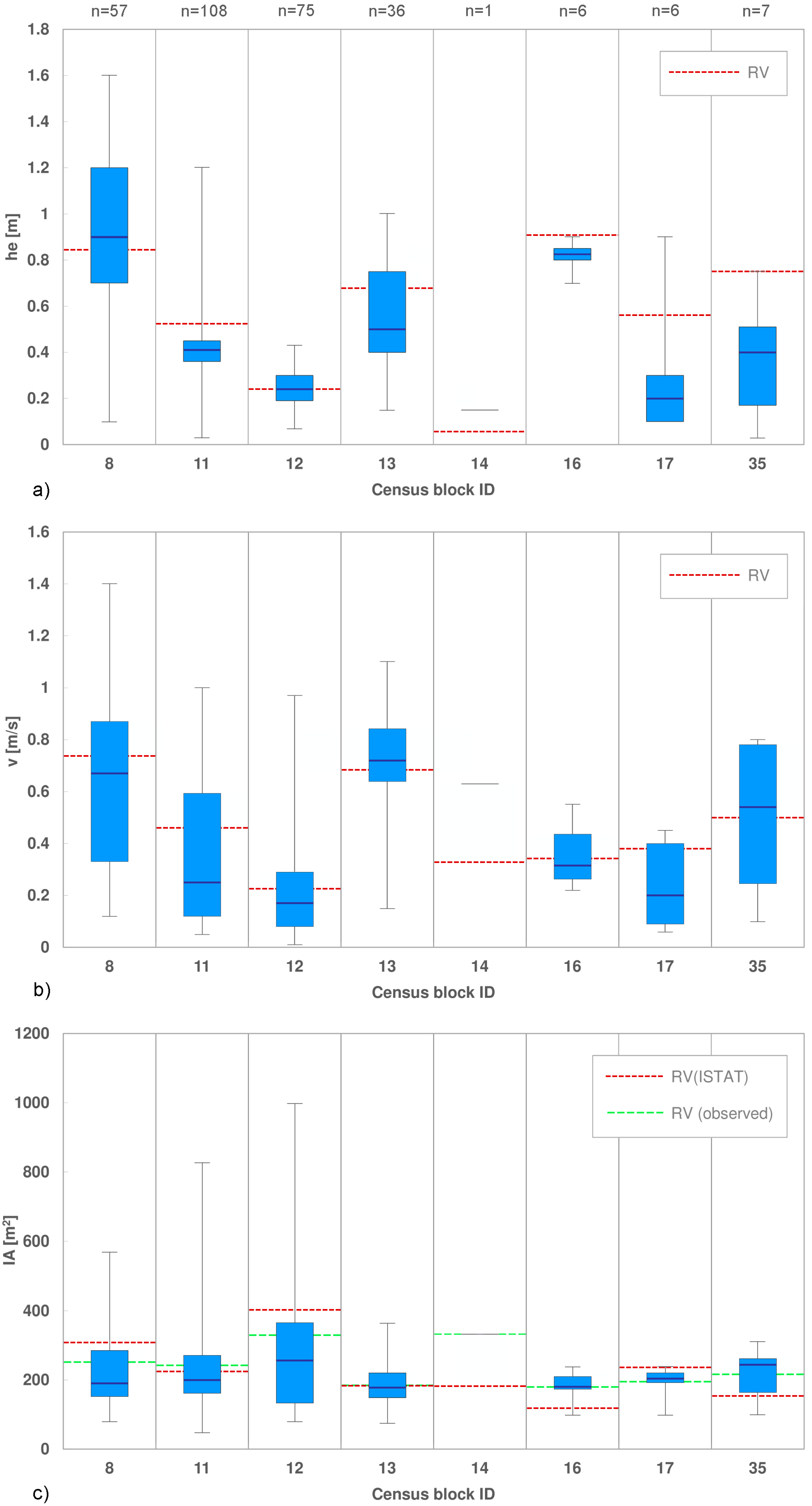
Moreover, it is interesting to compare Scenarios 1 and 2 to their homologous 3 and 5, which differ for the scale of representation of the event characteristic (micro- and census block scale), in order to analyse the influence of using RVs for the hazard variables. The boxplots in Figure 4 compare, for each census block, the variability of water depths and flow velocities registered at the building scale to the corresponding RVs calculated over each census block area. Excluding the census blocks with low representativeness, Figure 4 shows a good agreement between point and average flood characteristics, with maximum differences of about 10–20 cm (0.05–0.15 m/s) between the median of observed water depths (velocities) and the corresponding values averaged over the census block areas.
Therefore, given the uniform flood characteristics over the census blocks, the use of RVs for the event parameters in this case study induces a small error, ranging from 2% to 8%.
Furthermore, the comparison of the results of Scenarios 3 and 5 to the corresponding 4 and 6, with the last ones characterised by a lack of local knowledge of all parameters, including the footprint area, demonstrates the crucial role of information related to IA for flood damage assessments. Indeed, a significant increase in damage estimates is observed in all census blocks when using less detailed data (Figure 3, Scenarios 4 and 6), even in those blocks, as 11 and 13, which present the smallest differences between IA calculated based on ISTAT data and the median of observed micro-scale IA (Figure 4). For these two cases, when comparing Scenarios 3 to 4 and 5 to 6, an increment in the expected losses of about 40% and 60% is registered, respectively, for blocks 13 and 11. The maximum increment (up to 80%) is observed in block 8, characterised by a difference between the mean ISTAT IA and median observed IA of about 115 m2 (Figure 4).
Overall, the results of the analysis indicate that the error due to a partial knowledge of the input variables in INSYDE (i.e., implementation of a representative value for each parameter based on ISTAT data versus detailed micro-scale knowledge of the input variables) can be limited if two conditions are met: the representativeness of RVs with respect to local values and the accurate knowledge of the footprint area of the buildings. The first result is expected, while the second is justified by the fact that IA is the main “extensive” damage influencing variable in INSYDE [9].
Furthermore, the analysis reveals that the average and frequency criteria are almost equivalent for the definition of RVs for building variables, as demonstrated by the limited differences of performance indexes related to coupled scenarios (e.g., 1 and 2).
It is worth noting that the adoption of RVs for input variables coincides with a shift of the damage assessment from the micro- to the meso-scale. Indeed, with this study we have then investigated the usability of the INSYDE model at the meso-scale and, in particular, the consistency among the damage estimates supplied by the model at the two different scales. It is important to stress that, at present, most of existing models in the literature do not guarantee the coherence of results when applied at different spatial scales, mainly because they have been designed to work at a specific scale, without considering their up or down-scaling (few exceptions exist, e.g., FLEMO-ps [12] and the Multicoloured models [13]). From this perspective, INSYDE represents an advance to the state of the art, as it has been designed thinking about its possible implementation at upper scales rather than the local one [9].
Transferability of Results
As we do not expect many differences in the representativeness of ISTAT data at the national level, results can be extended to other Italian contexts, at least in regards to urban contexts and flood characteristics similar to the one analysed in this study. Nonetheless, other case studies are currently under investigation to corroborate the present main findings. On the contrary, the possibility of implementing INSYDE at the meso-scale in other countries must still be verified, as the typology and availability of aggregated data may change from country to country, as shown in Table 3.
With respect to this, the methodology described in this paper can be replicated in other physical and institutional contexts, in order to verify the representativeness of available aggregated data with respect to local data.
4. Conclusions
This short communication includes the preliminary results of a wider research aiming at exploring, by means of several case studies, the possibility of application of the micro-scale INSYDE model for flood damage assessment to residential buildings also at the meso-scale.
The analysis reveals that two conditions are required for limiting the errors in damage estimation when using coarse information available at an aggregated level instead of very detailed micro-scale input data: the representativeness of representatives values identified at the meso-scale, and the accurate knowledge of the footprint area of the buildings, being this parameter the main extensive damage influencing variable. This demonstrates the applicability of the INSYDE model not only at the micro- but also at the meso-scale, at least for the context investigated in the study (i.e., a flat medium-low density urban context with low velocity floods). However, other validation exercises in case studies characterised by different spatial and flood features are needed to generalise the results to other Italian and international contexts.
Acknowledgments
Authors acknowledge with gratitude all the other developers of INSYDE for their useful suggestions on this research.
Author Contributions
Authors are listed in alphabetical order. Authors contributed equally to this work.
Conflicts of Interest
The authors declare no conflict of interest.
References
- Merz, B.; Kreibich, H.; Schwarze, R.; Thieken, A. Assessment of economic flood damage. Nat. Hazards Earth Syst. Sci. 2010, 10, 1697–1724. [Google Scholar] [CrossRef]
- Apel, H.; Aronica, G.T.; Kreibich, H.; Thieken, A. Flood risk analyses—How detailed do we need to be? Nat. Hazards 2009, 49, 79–98. [Google Scholar] [CrossRef]
- De Moel, H.; Aerts, J.C.J.H. Effect of uncertainty in land use, damage models and inundation depth on flood damage estimates. Nat. Hazards 2011, 58, 407–425. [Google Scholar] [CrossRef]
- Freni, G.; La Loggia, G.; Notaro, V. Uncertainty in urban flood damage assessment due to urban drainage modelling and depth-damage curve estimation. Water Sci. Technol. 2010, 61, 2979–2993. [Google Scholar] [CrossRef] [PubMed]
- Jongman, B.; Kreibich, H.; Apel, H.; Barredo, J.I.; Bates, P.D.; Feyen, L.; Gericke, A.; Neal, J.; Aerts, J.C.J.H.; Ward, P.J. Comparative flood damage model assessment: Towards a European approach. Nat. Hazards Earth Syst. Sci. 2012, 12, 3733–3752. [Google Scholar] [CrossRef] [Green Version]
- Scorzini, A.R.; Leopardi, M. River basin planning: From qualitative to quantitative flood risk assessment: The case of Abruzzo Region (central Italy). Nat. Hazards 2017, 88, 71–93. [Google Scholar] [CrossRef]
- Molinari, D.; Menoni, S.; Aronica, G.T.; Ballio, F.; Berni, N.; Pandolfo, C.; Stelluti, M.; Minucci, G. Ex post damage assessment: An Italian experience. Nat. Hazards Earth Syst. Sci. 2014, 14, 901–916. [Google Scholar] [CrossRef]
- Cammerer, H.; Thieken, A.H.; Lammel, J. Adaptability and transferability of flood loss functions in residential areas. Nat. Hazard. Earth Syst. Sci. 2013, 13, 3063–3081. [Google Scholar] [CrossRef]
- Dottori, F.; Figueiredo, R.; Martina, M.L.V.; Molinari, D.; Scorzini, A.R. INSYDE: A synthetic, probabilistic flood damage model based on explicit cost analysis. Nat. Hazards Earth Syst. Sci. 2016, 16, 2577–2591. [Google Scholar] [CrossRef]
- Scorzini, A.R.; Frank, E. Flood damage curves: New insights from the 2010 flood in Veneto, Italy. J. Flood Risk Manag. 2015. [Google Scholar] [CrossRef]
- Chen, K.; McAneney, J.; Blong, R.; Leigh, R.; Hunter, L.; Magill, C. Defining area at risk and its effect in catastrophe loss estimation: A dasymetric mapping approach. Appl. Geogr. 2004, 24, 97–117. [Google Scholar] [CrossRef]
- Thieken, A.H.; Olschewski, A.; Kreibich, H.; Kobsch, S.; Merz, B. Development and evaluation of FLEMOps—A new Flood Loss Estimation Model for the private sector. In Flood Recovery, Innovation and Response; Proverbs, D., Brebbia, C.A., Penning-Rowsell, E., Eds.; WIT Press: Southampton, UK, 2008; ISBN 978-1-84564-132-0. [Google Scholar]
- Penning-Rowsell, E.C.; Johnson, C.; Tunstall, S.; Tapsell, S.; Morris, J.; Chatterton, J.; Coker, A.; Green, C. The Benefits of Flood and Coastal Risk Management: A Manual of Assessment Techniques; Middlesex University Press: London, UK, 2005; ISBN 1-904750-51-6. [Google Scholar]
Figure 1.
Schematisation of the processes for the definition of event and building parameters at the micro- and meso-scale (census block) level. (a) Upscaling of observed micro-scale inundation depths and flow velocities; (b) downscaling of building information from National Institute of Statistics (ISTAT) data to the micro-scale; and, (c) upscaling of observed micro-scale building information.
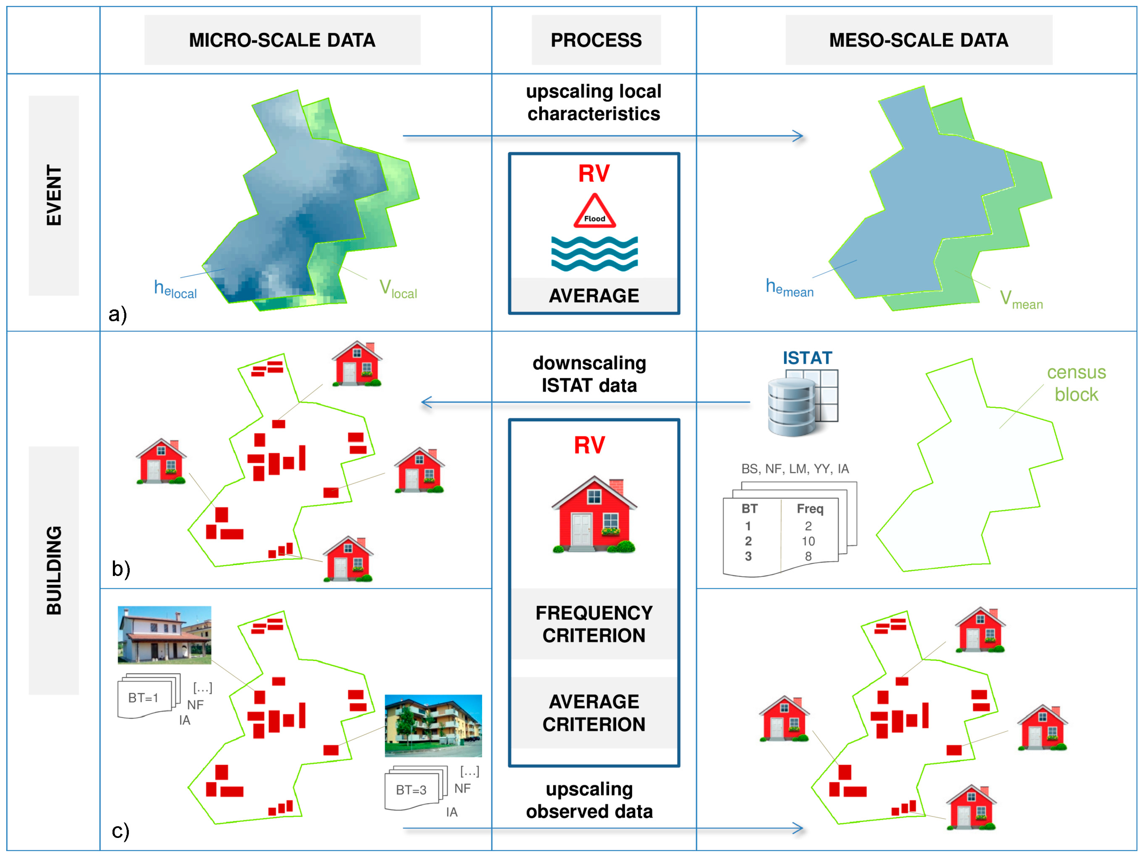
Figure 2.
Absolute frequencies of observed micro-scale data and identified representative value (RVs) with (i) frequency and average criterion and (ii) based on downscaling ISTAT data or on upscaling observed data.
Figure 2.
Absolute frequencies of observed micro-scale data and identified representative value (RVs) with (i) frequency and average criterion and (ii) based on downscaling ISTAT data or on upscaling observed data.
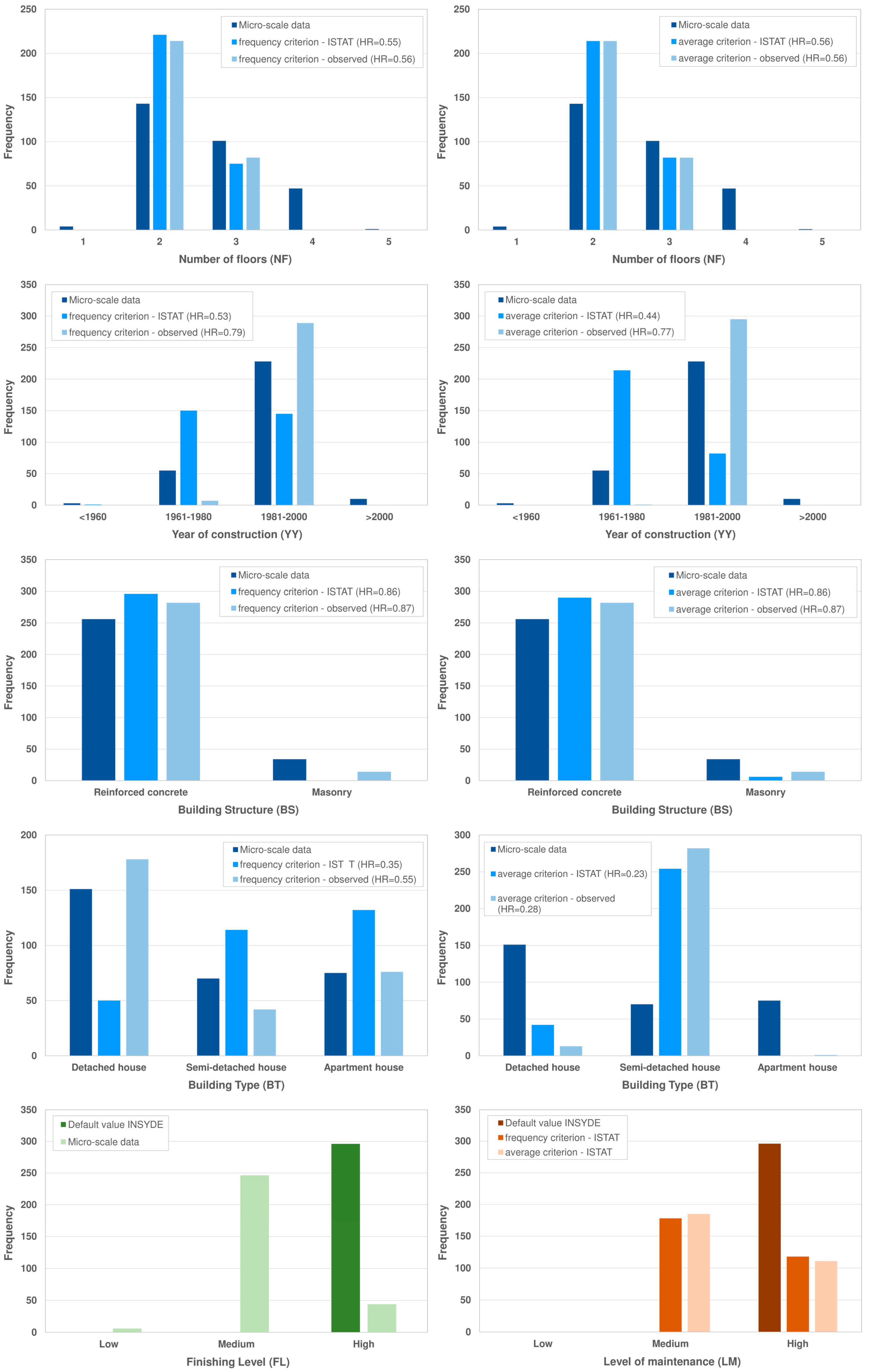
Figure 3.
Observed and estimated damages in each census block of the study area for the different scenarios (n indicates the number of affected buildings in each census block).
Figure 3.
Observed and estimated damages in each census block of the study area for the different scenarios (n indicates the number of affected buildings in each census block).
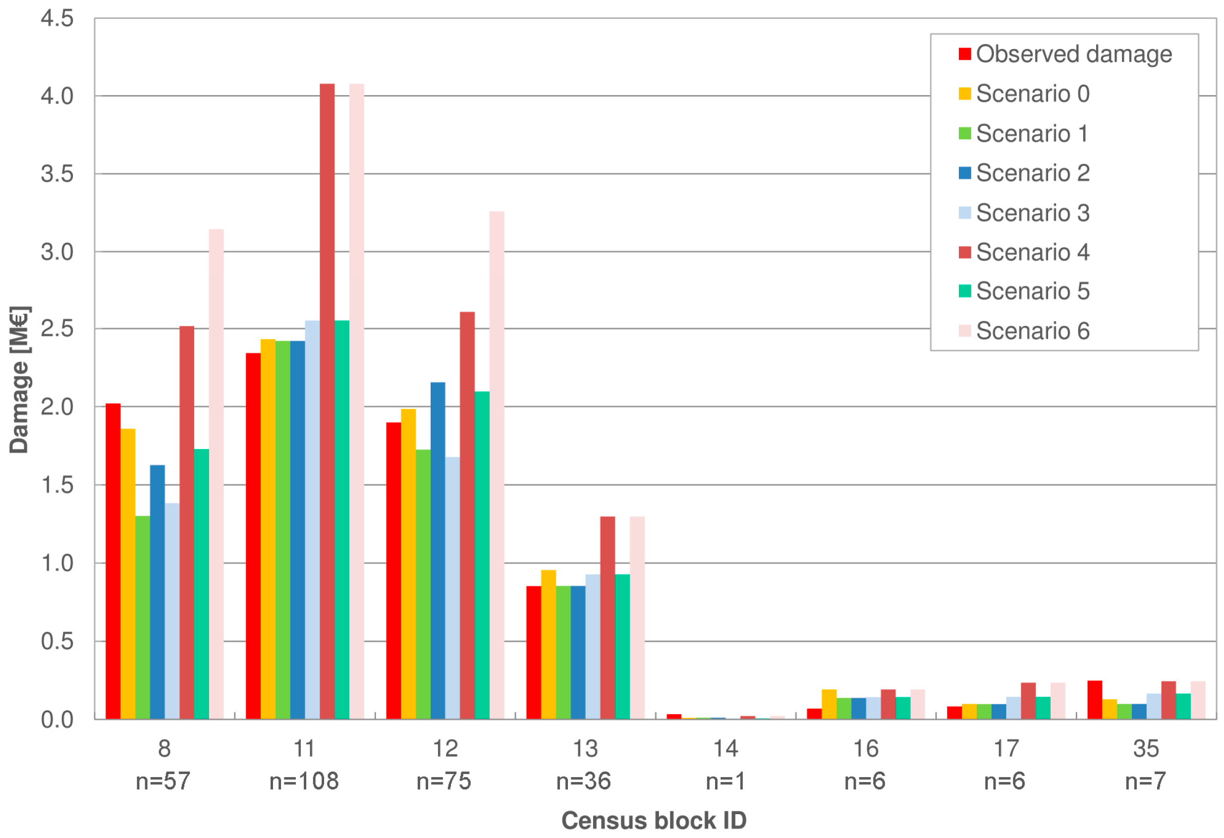
Figure 4.
Variability of micro-scale data compared to calculated RVs in each census block. Boxplots for (a) water depth; (b) flow velocity; (c) Internal area (n indicates the number of affected buildings in each census block).
Figure 4.
Variability of micro-scale data compared to calculated RVs in each census block. Boxplots for (a) water depth; (b) flow velocity; (c) Internal area (n indicates the number of affected buildings in each census block).

Table 1.
Input variables used in INSYDE and data type for the different scenarios (x = micro-scale information available; o = microscale information available (as a function of other variables, based on model’s assumptions); M = meso-scale information available; m = mesoscale information available (as a function of other variables).
| Event Features | Building Characteristics | ||||||||||||||||||||||
|---|---|---|---|---|---|---|---|---|---|---|---|---|---|---|---|---|---|---|---|---|---|---|---|
| External water depth (he) | Internal water depth (h) | Flow velocity (v) | Sediment load (s) | Duration (d) | Water quality (q) | Footprint area (IA) | Basement area (BA) | External perimeter (EP) | Internal perimeter (IP) | Basement perimeter (BP) | Number of floors (NF) | Interfloor height (IH) | Basement height (BH) | Ground floor level (GL) | Basement level (BL) | Building type (BT) | Building structure (BS) | Finishing level (FL) | Level of maintenance (LM) | Year of construction (YY) | Heat. syst. distrib. (PD) | Heat. syst. type (PT) | |
| Scenario 0 | x | o | x | M | x | x | o | o | o | x | x | x | x | x | o | o | |||||||
| Scenario 1 and 1a | x | o | x | M | x | o | o | M | M | M | M | M | m | m | |||||||||
| Scenario 2 and 2a | x | o | x | M | x | o | o | M | M | M | M | M | m | m | |||||||||
| Scenario 3 and 3a | M | m | M | M | x | o | o | M | M | M | M | M | m | m | |||||||||
| Scenario 4 and 4a | M | m | M | M | M | m | m | M | M | M | M | M | m | m | |||||||||
| Scenario 5 and 5a | M | m | M | M | M | m | m | M | M | M | M | M | m | m | |||||||||
| Scenario 6 and 6a | M | m | M | M | x | o | o | M | M | M | M | M | m | m | |||||||||
Table 2.
Estimated damages and performance indexes for the different scenarios (total reported damage for 2010 flood: 7.5 M€ in 296 buildings). Best and worst index values are highlighted in bold and italics, respectively.
Table 2.
Estimated damages and performance indexes for the different scenarios (total reported damage for 2010 flood: 7.5 M€ in 296 buildings). Best and worst index values are highlighted in bold and italics, respectively.
| Scenario | Dest [M€] | Bias | ME [€] | AME [€] | RMSE [€] | ||||
|---|---|---|---|---|---|---|---|---|---|
| ID | Water Depth (he) | Flow Velocity (v) | Internal Area (IA) | Other building Variables | |||||
| 0 | observed | observed | observed | observed | 7.66 | 1.01 | 370.3 | 17,483.8 | 28,907.9 |
| 1 | observed | observed | observed | RV-freq. (ISTAT) | 6.65 | 0.88 | −3044.7 | 16,310.0 | 27,658.6 |
| 2 | observed | observed | observed | RV-aver. (ISTAT) | 7.40 | 0.98 | −488.8 | 16,673.4 | 27,623.0 |
| 3 | RV | RV | observed | RV-freq. (ISTAT) | 7.00 | 0.93 | −1864.1 | 17,663.8 | 28,606.9 |
| 4 | RV | RV | RV | RV-freq. (ISTAT) | 11.19 | 1.48 | 12,309.9 | 24,064.7 | 31,420.1 |
| 5 | RV | RV | observed | RV-aver. (ISTAT) | 7.76 | 1.03 | 720.8 | 18,246.8 | 28,692.7 |
| 6 | RV | RV | RV | RV-aver. (ISTAT) | 12.47 | 1.65 | 16,636.1 | 26,640.8 | 33,290.2 |
| 1a | observed | observed | observed | RV-freq. (observed) | 6.97 | 0.92 | −1953.1 | 16,267.0 | 27,426.8 |
| 2a | observed | observed | observed | RV-aver. (observed) | 7.40 | 0.98 | −496.5 | 16,681.0 | 27,629.3 |
| 3a | RV | RV | observed | RV-freq. (observed) | 7.34 | 0.97 | −700.3 | 17,832.9 | 28,487.3 |
| 4a | RV | RV | RV | RV-freq. (observed) | 11.01 | 1.46 | 11,701.2 | 24,061.2 | 31,539.5 |
| 5a | RV | RV | observed | RV-aver. (observed) | 7.76 | 1.03 | 716.7 | 18,251.0 | 28,696.7 |
| 6a | RV | RV | RV | RV-aver. (observed) | 11.54 | 1.53 | 13,478.3 | 24,768.7 | 31,888.9 |
Table 3.
Availability of aggregated building data in some European countries at census block or municipality level (information obtained from the databases of the National Institutes of Statistics of the different Countries).
Table 3.
Availability of aggregated building data in some European countries at census block or municipality level (information obtained from the databases of the National Institutes of Statistics of the different Countries).
| Country | Level of Detail | Available Variables |
|---|---|---|
| Italy | Census block | NF, BT, BS, YY, LM |
| UK | Census block | BT, PD |
| France | Census block | IA, YY, PD |
| Spain | Census block | IA, NF, YY, LM |
| Belgium | Municipality | YY, LM |
| Germany | Municipality | YY, IA, BT, PD |
| Portugal | Municipality | NF, IA |
© 2017 by the authors. Licensee MDPI, Basel, Switzerland. This article is an open access article distributed under the terms and conditions of the Creative Commons Attribution (CC BY) license (http://creativecommons.org/licenses/by/4.0/).
Share and Cite
MDPI and ACS Style
Molinari, D.; Scorzini, A.R. On the Influence of Input Data Quality to Flood Damage Estimation: The Performance of the INSYDE Model. Water 2017, 9, 688. https://doi.org/10.3390/w9090688
AMA Style
Molinari D, Scorzini AR. On the Influence of Input Data Quality to Flood Damage Estimation: The Performance of the INSYDE Model. Water. 2017; 9(9):688. https://doi.org/10.3390/w9090688
Chicago/Turabian StyleMolinari, Daniela, and Anna Rita Scorzini. 2017. "On the Influence of Input Data Quality to Flood Damage Estimation: The Performance of the INSYDE Model" Water 9, no. 9: 688. https://doi.org/10.3390/w9090688
Note that from the first issue of 2016, this journal uses article numbers instead of page numbers. See further details here.