Adapting the Relaxed Tanks-in-Series Model for Stormwater Wetland Water Quality Performance

1
Biological & Agricultural Engineering, North Carolina State University, Campus Box 7625, Raleigh, NC 27695, USA
2
Civil and Environmental Engineering, University of Tennessee, 415 John D. Tickle Building, Knoxville, TN 37996-2010, USA
*
Author to whom correspondence should be addressed.
Water 2017, 9(9), 691; https://doi.org/10.3390/w9090691
Submission received: 15 July 2017
/
Revised: 18 August 2017
/
Accepted: 4 September 2017
/
Published: 9 September 2017
(This article belongs to the Special Issue Treatment Wetlands for Nutrient Removal)
Abstract
:Across the globe, water quality standards have been implemented to protect receiving waters from stormwater pollution, motivating regulators (and consequently designers) to develop tools to predict the performance of stormwater control measures such as constructed stormwater wetlands (CSWs). The goal of this study was to determine how well the relaxed tanks-in-series (P-k-C*) model described the performance of CSWs in North Carolina. Storm events monitored at 10 CSWs in North Carolina were used for calibrating the model, and statistical evaluations concluded the model could adequately predict the performance for all pollutants except organic nitrogen. Nash–Sutcliff calibration/validation values were determined to be 0.72/0.78, 0.78/0.74, 0.91/0.87, 0.72/0.62, 0.88/0.73, and 0.91/0.63 for total nitrogen, total ammoniacal nitrogen, oxidized nitrogen, organic nitrogen, total phosphorus, and total suspended solids, respectively. Sensitivity analysis revealed only one calibration parameter with strong sensitivity, the Arrhenius coefficient (temperature dependent model coefficient). With this model, CSWs can be optimized to treat watershed-specific influent concentrations to meet effluent targets. In general, the current design technique used in North Carolina and many other locations (a first flush volume detention method) oversizes CSWs for water quality vis-à-vis the method herein, suggesting improved designs for water quality may be possible through scientifically-informed methods.
Keywords:
stormwater; wetlands; kinetics; water quality; hydrodynamics; modeling; design; rate constant1. Introduction
Constructed stormwater wetlands (CSWs) have become one of the more commonly utilized stormwater control measures (SCMs) [1,2,3,4]. A well-functioning CSW has an ecosystem with diverse plant and animal species that also removes water-borne pollutants (source). Most regulatory entities set design standards to capture and detain the water quality volume of runoff, which is released over two to five days and subjected to treatment during the inter-event period [5,6]. If these design requirements are met, pollutant removal credits for total nitrogen (TN), total phosphorus (TP), and total suspended solids (TSS) of 40%, 40%, and 85%, respectively, are granted in North Carolina (NC), with similar removal credit systems being in place in other municipalities in the United States [7]. This sizing methodology implies a degree of treatment that may not be accurate, necessitating more mechanistic approaches to accurately size and credit CSWs when water quality reduction is the primary goal.
Research performed on CSWs suggests that substantial water quality improvement may be possible in smaller systems. Hathaway and Hunt (2010) [2] studied the water quality treatment of three CSW cells in series near Charlotte, NC, USA. The authors observed at least 80% of the total concentration reduction occurred within the first wetland cell for all pollutants examined, concluding that successive CSWs did not provide substantially more concentration reduction. Likewise, Merriman et al. (2016) [8] examined the treatment performance of a 17-ha CSW located in the Coastal Plain of North Carolina for two pumped flow regimes: event and base flow. The multiple cell design produced a treatment train where, similar to Hathaway and Hunt (2010) [2], at least 80% of treatment for storm events occurred in the first cell with little additional treatment in subsequent cells. These research findings suggest that current design methodologies might be oversizing CSWs with respect to discharge concentrations, and that further optimization is possible with more sophisticated design tools (such as a predictive model).
Further, CSW performance has been shown to be highly variable in North Carolina applications (Table 1). Thus, there are additional parameters critical to performance that are not given consideration in simple water quantity based designs. Factors such as influent pollutant concentration have been shown to affect CSW performance, and could be utilized in a modeling framework to allow realistic predictions of performance [9].
A strong body of knowledge is available for analogous installations of free surface water constructed wetlands for wastewater treatment, hereafter referred to as “treatment wetlands”. Such installations have proven to be successful since their introduction as a water treatment technology in the 1970s [3,13]. For 40 years, water quality data have been collected from treatment wetlands, with the finding that the rate of concentration reduction for pollutants is well represented by first order (the k-C* model) decay kinetics [13,14,15]. Subsequently, these first order decay functions have been adapted to event-driven, CSW, systems [14,16,17]. Although Kadlec and Knight (1996) [16] reasoned the plug flow assumption associated with the k-C* model might not be representative of the actual hydrodynamics in CSWs, using the model did provide a conservative estimate of treatment performance provided background concentrations were considered. The k-C* model is often used as an interpolator on data sets, but difficulties arise when the model extrapolates outside of the calibrated concentration ranges, or for comparing design configurations [18]. Thus, although the k-C* model is simple and widely used, it fails to adequately characterize the complex processes that occur in treatment wetlands or CSWs [19].
More recently, the P-k-C* reaction rate model (relaxed tanks-in-series, PTIS, reaction rate model) was adapted to stormwater applications by Wong et al. (2006) [20]. This model has been endorsed because it accounts for velocity (i.e., short-circuiting and stagnant zones) and reaction rate heterogeneity (i.e., concentration weathering) in wetlands, while using a minimal number of parameters [3,21]. However, there has not been an effort to investigate the applicability of this model on CSWs utilizing field-based data, a critical need before this more scientifically informed method of CSW design for water quality can be widely utilized. Thus, the goal of this study was to determine the ability of the P-k-C* model to describe the treatment response of CSWs in North Carolina and demonstrate its application as a design optimization tool.
2. Materials and Methods
2.1. Model Description
During unsteady flows (descriptive of stormwater systems), water quality varies as “parcels” of variably treated water passes through a CSW [3]. To more thoroughly describe CSW treatment, it is necessary to simultaneously consider both pollutant depletion and flow hydrodynamics [3]. The Tanks in Series (TIS) model (Equation (1)) applies a combination of the k-C* model and the continuously stirred tank reactor (CSTR) model to adequately describe both pollutant depletion and flow hydrodynamics [3,20,22]. This model assumes steady state conditions: no infiltration, no evapotranspiration, and constant flow while this parcel of water is in the wetland. Despite this assumption not truly reflecting field conditions, the TIS and k-C* models have been widely and successfully used to predict discharge concentrations in treatment wetlands [21,23,24].
where Cout = effluent concentration (mg/L), Cin = influent concentration (mg/L), C* = background concentration in the wetland (mg/L), kT = reaction rate constant (m/year) at ambient Temperature, T (°C), = detention time (d), N = tracer test determined number of tanks in series (TIS), and h = wetland free water depth (m).
Per previous studies [1,3,19,21,22,25,26,27], N, kT, and C* model inputs can be relaxed to model fitting parameters: P, kT,app (apparent reaction rate constant), and C*. This forms the relaxed TIS model (PTIS or P-k-C* model). Because the P-k-C* method encompasses the final concentration profiles from a variety of causative distributions, it better represents multiple situations [3,21]. Nitrogen and phosphorus biogeochemical removal mechanisms and their rate constants are temperature sensitive [3,21,28,29]. The modified Arrhenius equation (Equation (2)) describes temperature dependence and is often combined with reaction models for model calibrations [3,21,28]. A θ value = 1.000 indicates temperature does not affect treatment, while values below or above 1.000 signify a negative or positive effect on treatment, respectively, at higher temperatures [3].
where kT = removal rate constant (m/year) at water temperature, T (°C), k20 = removal rate constant at 20 °C (m/year), and θ = dimensionless temperature coefficient.
The result of combining Equations (1) and (2) utilizing model filling parameters is presented in Equation (3). This model combines the first order decay function with a reaction model and coefficient adjustment to account for varying hydrodynamics (decay function) and temperature (coefficient adjustment) (Equation (3)).
2.2. Determination of Input Parameters
2.2.1. Site Description
2.2.2. Monitored Influent (Cin) and Effluent (Cout) Concentrations
The methods used to collect and analyze water samples were similar among studies: flow-paced water quality samples were collected from the inlets and outlets of all CSWs using ISCO automatic samplers such that nutrient and sediment event mean concentrations (EMC) could be determined (Table 3). Analytes from each site included total ammoniacal nitrogen (TAN), nitrite-nitrate nitrogen (NO2,3-N), TP, and TSS. Organic nitrogen (ON) concentrations were calculated by subtracting TAN from total Kjeldahl nitrogen (TKN) measurements for individual storm events. Total nitrogen concentrations were also calculated by adding TKN and NO2,3-N values for each storm event.
2.2.3. Background Concentrations (C*)
Background concentrations (C*) were developed by combining data from CSW literature and previous studies that applied first order decay models on treatment wetlands. Treatment wetland modeling studies typically assumed that the background concentrations for TP, NO2,3-N, and TAN were zero [3,23]. Conversely, using effluents of CSWs and a reference natural wetland in North Carolina, Moore et al. (2011) [33] determined the background concentration for ON to range from 0.7 to 0.8 mg/L. The minimum observed effluent TSS concentration (2 mg/L) was used for the TSS background concentration. Seasonal variations (temperature) were not considered for the background concentration estimates in this analysis.
2.2.4. CSW Design Characteristics
The detention time, τ, and free water depth, h, are assumed to remain relatively constant for treatment wetlands, but for CSWs, these parameters depend on antecedent conditions and vary from event to event [20,27]. The average free water depth and detention time for the water quality storm event (25 or 38 mm) reported for each CSW (Table 4) were used for this analysis.
2.2.5. Water Temperature (T)
Since water temperature was not measured for any of the CSWs, data were compiled from U.S. Geological Survey (USGS) stream stations located closest to each CSW [34]. Although stream water temperatures are most likely to be less than those observed in CSWs, this was the best available estimate of this parameter. The historical mean monthly water temperatures (°C) of each station were calculated; CSW storm events were assigned a water temperature, on a monthly basis, from the nearest USGS station. Temperatures ranged from 3.3 °C in January at the Asheville, NC (Mountains) station to 31.3 °C in July at the Falls, NC (Piedmont) station.
2.3. Model Calibration, Validation, and Sensitivity Analysis
Data from the CSWs were parsed into individual storm events and divided into calibration and validation datasets by assigning odd numbered events (per chronological order) to the calibration dataset and even numbered events to the validation dataset. This method provided a seasonal representation for the calibration and validation datasets for each CSW. For situations when there were not an adequate number of events for both model calibration and validation (i.e., n < 8), all events were used for calibration.
Calibration parameters; k20, P, and θ, were found by fitting the modeled data to the observed and minimizing the root mean squared error (RMSE in mg/L) between observed effluent concentrations (Oi) and modeled effluent concentrations (Pi) by simultaneous adjustment of k20, P, and θ for all events, n [19,28]. In addition to the RMSE, the coefficient of determination, R2, and Nash–Sutcliffe efficiency, NSE [35] were used as statistical performance measures for the model. The NSE was selected as a dimensionless goodness-of-fit indicator.
Sensitivity of fitting parameters (P, k20, and θ) was explored using a Monte-Carlo approach, with parameter ranges being developed from literature and the calibration outcomes in this study. For each pollutant, 250,000 simulations were conducted using the Nash–Sutcliffe coefficient as the objective function. Parameter distribution plots were generated for each CSW individually and all CSW data collectively based on the acceptable parameter sets identified in the analysis, allowing an understanding of the sensitivity of the model to each parameter.
3. Results
3.1. Individual CSW Calibration and Validation: Resultant Reaction Rate Parameters
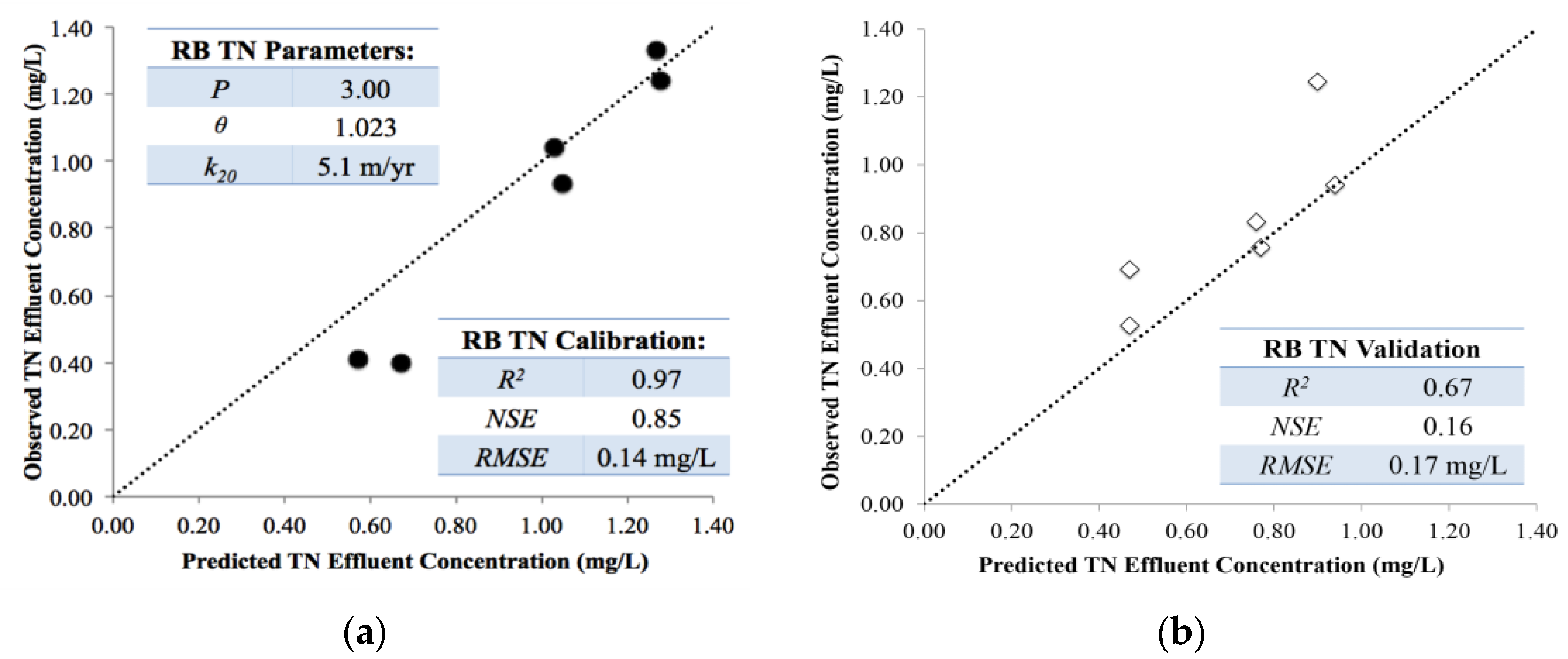
Modeling fitting (reaction rate) parameters and statistical evaluations were generated for both calibration and validation datasets for each pollutant and CSW (Figure 2). The reaction rates for each evaluation are summarized in Table 5.
The apparent number of TIS (P) ranged from 1.4 to 7.6 for each pollutant and CSW (Table 6). This range fell well within the scope of tanks in series values (1–10) derived from conservative tracer experiments compiled by Kadlec and Wallace (2008) [3] and simulations conducted by Persson et al. (1999) [36] for treatment wetlands. The mean and median P values ranged from 3.0 to 4.0 (Table 5), similar to the value (3.0) recommended for initial modeling estimates and for use in treatment wetland design [3,36,37]. Overall, the CSW sites with lower P values (EB, DB, and JSC1), indicative of well-mixed hydrodynamics, had longer detention times relative to the other sites (Table 4). Higher P values suggested more short-circuiting and, typically, corresponded with deeper storage depths (CMS and Bass, Table 4), where interactions with soil and vegetation are minimized and limit flow retardation and treatment potential [4,27,36,38].
The temperature coefficients (θ) for pollutants derived from the field investigations varied for each CSW. The mean values for TN, TAN, TP, and TSS demonstrated temperature effects to be negligible with values of 1.007, 1.002, 1.002, and 0.993, respectively (Table 5). In relatively warm climates, such as North Carolina, no temperature effect on TP performance has typically been observed [3,28,39], and variability in TSS treatment is not usually attributed to temperature [3]. The lack of effect of temperature on TN and TAN treatment was surprising since it has been well-documented that nitrogen processes are influenced seasonally [21,28,29,39]. However, when the TN and TAN loading to a wetland is substantially less than the growth requirements of the plants and algae (<120 and 108 g/m2/year, [3]), the removal of TN and TAN is mediated by the growth and decay of biomass [29,40]. Plant uptake rates peak in the spring and do not correspond to the annual cycle of water temperatures [3,29]. Therefore, in lightly loaded CSWs, water temperature and modified Arrhenius θ values have no effect on TN and TAN removal. The mean θ for NO2,3-N and ON (1.024 and 1.034, respectively) reflected greater treatment at higher temperatures (Table 6). Kadlec (2010) [37] observed θ values ranging from 1.035 to 1.113 for NO2,3-N treatment in Ohio similar to that (1.043) observed in New Hanover County, NC [3]. Stanford et al. (1973) [41] found θ values for ON ranged from 1.07 to 1.08, while Marion and Black (1987) [42] observed θ = 1.08–1.16. The NO2,3-N and ON temperature effects herein were not as prominent as these studies. This was attributed to the smaller range of annual water temperatures observed at the USGS stream station.
The rate constants (k20) derived from the calibration exercises resulted in a large range for each pollutant (Table 5). The upper range primarily consisted of rate constants found for the NCSU, JSCA, UNCA sites. These sites had higher influent concentrations compared to the sites with lower k20 values (RB and BES). Because these rate constants describe the rate a wetland can treat influent concentrations to selected background concentrations, higher values are expected for higher influent concentration. This trend does not hold when comparing rate constants for CSWs to those of treatment wetlands. The mean rate constants found in this study were higher than those found for treatment wetlands (Table 6). For example, nitrogen values equated to the 91st (phosphorus, the 84th) percentile in the distribution of treatment wetland rate constants compiled by Kadlec and Wallace (2008) [3]. Although treatment wetlands have higher influent concentrations compared to CSWs, treatment wetlands tend to have longer detention times and steady flow conditions compared to the flashy, episodic nature of stormwater systems [27,36]. Constructed stormwater wetlands yield a higher “rate of treatment” given the flashiness of their hydrology, demonstrating that rate constants are also a function of detention time and hydrodynamics (rather than solely on influent concentrations). This supports Kadlec (2010) [37] where NO2,3-N dynamics in pumped riverine wetlands for pulsed vs. steady flow conditions were evaluated. Rate constants observed were much higher for pulsed flow than for steady state conditions (k20 = 107 vs. 37 m/year). The same was observed for TP in Kadlec (2001) [43] with k20 = 212 vs. 88 m/year for pulsed flow and steady state conditions, respectively. Few studies have been conducted to find rate constants for CSWs. Carleton et al. (2001) [17] summarized rate constants for TP, TAN, and NO2,3-N in 18 studied constructed wetlands receiving urban runoff. Rate constants for TP ranged from 4.9 to 46.7 m/year aligning with that observed herein (38.0 m/year), but the ranges for NO2,3-N and TAN (3.6–57.1 and 1.0–24.6 m/year, respectively) were less than that found here (65.5 and 37.5, respectively: Table 6). For wetlands with varying ponded surface areas and volumes, such as CSWs, Carleton et al. (2001) [17] based their calculations on maximum values of these parameters to generate maximally conservative (that is, minimal) estimates of rate constants. This methodology could explain why their reported k20 values were, overall, less than those derived in this study.
3.2. Calibration and Validation Results
Statistical evaluations were compiled for calibration and validation datasets for each pollutant and CSW (Table 7 and Table 8, respectively). Wong et al. (2006) [20] reported the ability of a unified model (P-k-C*) to predict stormwater treatment of various SCMs, and although no rate constants were provided, TN, TP, and TSS model fits (RMSE = 0.08, 0.03, and 6.9 mg/L, respectively) supported this conclusion. Similar findings were observed in this study with RMSE averages of 0.21, 0.02, and 6.85 mg/L for TN, TP, and TSS, respectively (Table 7). The RMSE for TN was higher than that found by Wong et al. (2006) [20], but given the range of influent concentrations and CSW designs, the RMSE was still relatively low. Total nitrogen and TP validation RMSE values were similarly low: 0.20 and 0.04 mg/L, respectively; however, the RMSE for TSS increased to 21.19 mg/L. This increase was attributed to the poor fit of one CSW, NCSU (RMSE = 124.4 mg/L). The median was similar to results found during calibration (6.59 mg/L).
The average R2 statistics indicated that the model explained 65–77% of the total variance in observed effluent concentrations for all pollutants (Table 8). This range widened for the validation datasets where 24–77% of observed concentration variability was explained by the model (Table 8). Nash-Sutcliffe model efficiency values across all pollutants ranged from 0.46 to 0.73 and −4.32 to 0.31 for calibration (Table 7) and validation (Table 8), respectively, where a negative NSE signified the observed mean effluent concentration was a better predictor of effluent concentrations than the model. Both of these statistical parameters are sensitive to extreme events [44], commonly found in the relatively small sample size of events (i.e., n < 8) for each individual CSW’s calibration and validation datasets.
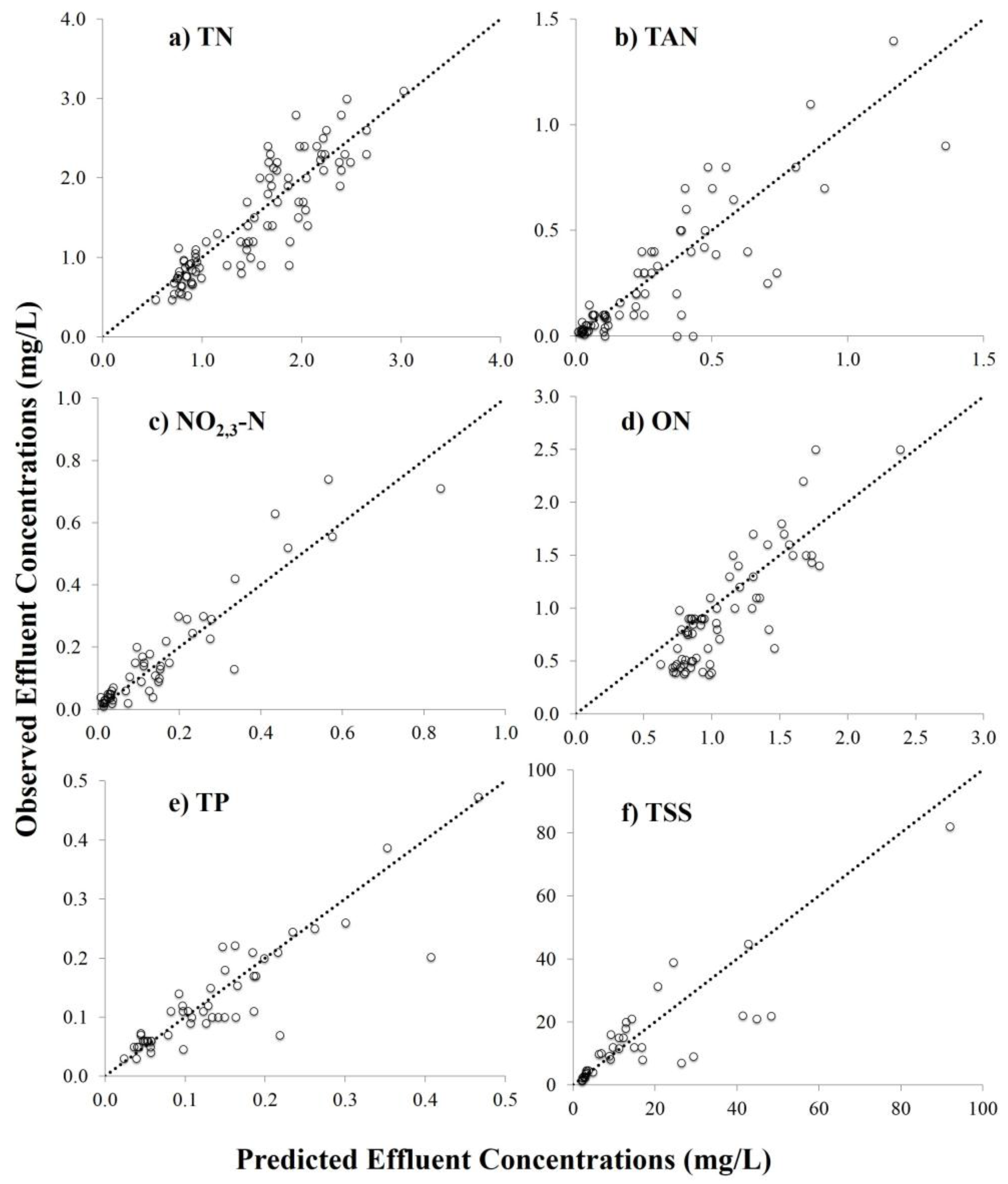
Plots demonstrating observed vs. predicted relationships for pollutant effluent concentrations from model calibration and validation events across all CSWs are compiled in Figure 3a–f and Figure 4a–f, respectively. Essentially, the CSWs were modeled, calibrated, and validated individually before the observed/predicted values were recompiled for an overall calculation of RMSE and NSE. The statistical metrics of all compiled CSW results for each pollutant are summarized in Table 9.
Model prediction strength varied between calibration and validation. While events were randomly assigned to the calibration and validation data sets, those data sets were in some cases surprisingly dissimilar. For example, the TSS calibration (Figure 3f) and validation (Figure 4f) dataset distributions were different, even though these datasets were chosen at random. Regardless, the P-k-C* model was typically able to describe the observed behavior well. These results: (1) suggest there is an underlying unity of a number of complex processes; and (2) support the model’s intended use for conceptual analysis and as a design tool. As an early attempt to calibrate the P-k-C* model for use in many varying CSWs, these initial results are promising.
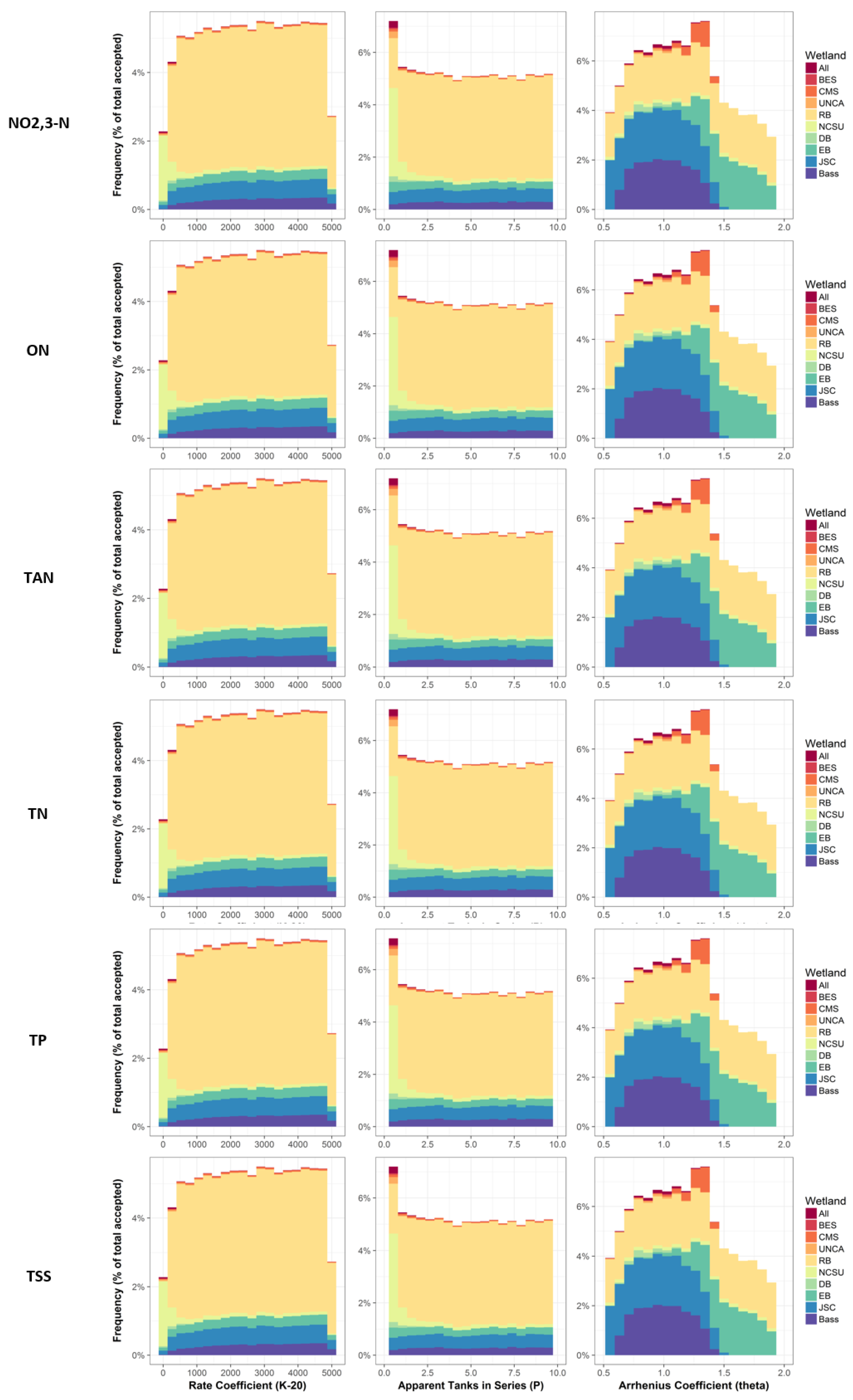
3.3. Sensitivity Analysis Results
The results of the sensitivity analysis are presented in Figure 5. The distributions found for the Arrhenius coefficient, θ, indicate that the model outputs were sensitive to the change in this parameter, where a θ value of approximately 1.0 was the optimized value, although some wetlands’ optimized values were closer to approximately 1.5. The mean calibrated θ values determined for CSWs in NC (Table 5) fall within the optimized range determined by the sensitivity analysis (Figure 5) and values determined by previous studies. Kadlec and Wallace (2008) [3] cataloged θ values of 1.002, 1.078, 1.082, and 1.043 for TP, ON, TN, and NO2,3-N, respectively, for a wetland system studied in New Hanover County, NC. For TAN, a coefficient of 1.040 was used by Stone et al. (2002) [28] for a livestock treatment wetland located in Duplin County, NC. Finally, total suspended solids concentration time series often display some degree of sinusoidal behavior, similar to nitrogen and phosphorus, through the course of a calendar year; however, variability in performance has not been attributed to temperature [3]. Therefore, a temperature coefficient for TSS of 1.000 is appropriate.
The lack of a defined peak in the distribution for both P and k20 suggests that model outputs were not sensitive to these parameters. Kadlec and Wallace (2008) [3] compiled tracer response curves for several surface flow treatment wetlands and found them all to be reasonably represented by P = 3, in spite of their different geometries. Likewise, a wetland with a meandering low flow channel with full vegetation was best described as P = 3.1 TIS in Melbourne, Australia [36]; as was NO2,3-N treatment in event-driven wetlands [37]. Wong and Geiger (1997) [14] suggested rate constants for TN and TSS of 22 and 1000 m/year, respectively, based on 59 treatment wetland systems. Carleton et al. (2001) [17] narrowed this range in a study of removal rate constants (k20) for 19 constructed wetland systems receiving urban runoff. Lack of sensitivity in k20 was a surprising result. The consistent concentrations and detention times, which were relatively less than typical values for treatment wetlands, could explain why k20 was not found to be sensitive in the model, which was a surprising result. The mean, calibrated values for P and k20 determined in this study (Table 5) were similar those observed in these previous studies, supporting the wide use of these mean values due to their lack of sensitivity on model outputs. That is, these parameters can possibly be set by literature values and no longer require calibration.
4. Discussion
The practice of stormwater wetland design for water quality improvement is in need of more scientifically-informed methods. Fortunately, there is a strong base of literature to rely on from analogous treatment wetland studies which have primarily targeted wastewater. However, most literature and design methods continue to use the plug flow based k-C* model and univariate analysis, where a single number is used to describe a parameter such as a detention time or rate constant. However, treatment and stormwater wetland variables and parameters do not possess single unique values, but rather a distribution of these values with respect to a wetland attribute [1,3,21]. Wetland detention time distributions alone are often responsible for departures from plug flow behavior [18,19,21], thus affecting the transferability of these models outside their treatment wetland calibration envelops or even to the stochastic nature of CSWs. Kadlec (2003) [21] demonstrated the combination (P-k-C* model) of first-order decay kinetics with a CSTR batch model could adequately embody wetland parameter distributions. This was imperative for the transferability of the model among CSWs with variable design characteristics, detention times, and influent concentrations.
For most pollutants investigated, the P-k-C* kinetic model was able to describe the observed behavior quite well, with the exception of ON, which was not necessarily unexpected given internal residuals and wetland return fluxes [29,33]. These results suggested there is an underlying unity of a number of complex processes and supported the model’s intended use for conceptual analysis and as a design tool. Wong et al. (2006) [14] drew the same conclusions when utilizing the model across various SCMs with differing pollutant removal mechanisms.
After model calibration to achieve CSW-centric reaction rate parameters (namely k20 and P), rearrangement of the P-k-C* model lends designers the ability to solve for the detention time or area required to achieve a target effluent concentration. Designer inputs include watershed-specific influent concentrations for pollutants of concern, effluent targets, design storm event size, and the CSW’s design free water depth.
Considering this is one of the first attempts to calibrate the P-k-C* model to numerous individual field-scale runoff events across many CSWs, the results were deemed successful, but also provide a focus for future research to enhance the model. The first priority for such research would be to incorporate storm events from CSWs monitored long term. The age range (1–5 years) for calibrated CSWs in this study was relatively small and primarily consisted of “young” systems. It is imperative to test the applicability of the model for not only different catchments and design characteristics but also different ages. Stochastic effects on treatment, especially in CSWs, could mask the seasonal behavior of a wetland system [39]; therefore, analyzing several years of data to develop seasonal trends in performance is important in accurately establishing temperature coefficients. Further research into the hydrodynamics of CSWs by conducting conservative tracer tests would provide insights into detention time distributions. These tests could also establish field-based short-circuiting/mixing parameters (N) instead of finding these values empirically (P).
The complexity of modeling wetland processes has created two distinctly different reactions among practitioners [21]. Wetland scientists argue for greater quantification and utilization of data and details [45,46], but offer no mechanisms for incorporating that detail or data into practical wetland design [21]. Practitioners and regulators condemn the “black box” approach, but reject detailed modeling methods in favor of practicality [21,47]. The tradeoff between model accuracy and calibration data requirements is difficult. The most reliable prediction of pollutant removal for given event in a specific CSW will be provided by a more detailed model, but often at the expense of extensive calibration requirements. Use of the P-k-C* model minimizes the parameters to be calibrated (k20, θ, and P), as demonstrated in this study for CSWs in North Carolina, while also offering the ability to embody the weathering behavior of concentrations and deviation from plug flow observed in real wetland systems. Further, the analysis herein suggests that two of these calibration parameters may be reduced to literature values based on their relative lack of sensitivity. This is important if designers are to use this as a design tool across a range of catchments.
Greenway (2004) [4] argued the area of a CSW should be a function of catchment size, the volume of runoff, pollutant characteristics of the runoff, the desired level of water treatment, and the extent to which the CSW was also expected to function as a retention basin. Currently, the design method in North Carolina only considers catchment size, volume of runoff, and peak flow mitigation, but the application of the P-k-C* model can assist practitioners in including runoff pollutant characteristics and the desired level of water treatment. Many studies recommend performance metrics other than percent removal should be employed for SCMs [48,49,50]. Strecker et al. (2001) [48] stated that biological and downstream habitat assessment should be explored as an assessment technique, and McNett et al. (2010) [51] reasoned that evaluating SCMs in context with the environment in which they are located may be as valid a way of measuring how well they are functioning as the currently used concentration and load based metrics. Design of CSWs could also follow this same reasoning by optimizing designs to treat watershed-specific influent concentrations to target effluent thresholds based on receiving waterbodies.
Steady state conditions, no gains or losses, is one main underlying assumption of the P-k-C* model. Volume reductions in CSWs are typically negligible [8,12,52]; however, some systems have experienced significant reductions (24–55%) due to seepage and evapotranspiration [8,50,53,54]. Consequently, CSW designs based on this model would provide conservative area recommendations, and further refinements to the model could include water balance calculations to evaluate CSW performance and sizing on a mass loading basis.
5. Conclusions
The goal of this study was to determine the ability of the P-k-C* model to describe the treatment response of CSWs in North Carolina, and demonstrate its application as an optimization tool for designing CSWs. Such methods will aid in advancing the science of stormwater management beyond a “black box” understanding of internal SCM processes, allowing more scientifically-informed design. Storm events monitored at 10 CSWs in North Carolina were used to determine reaction rate parameters through model calibration exercises. Statistical evaluations concluded that the P-k-C* model could accurately describe the water quality treatment response for all pollutants except organic nitrogen, due to complex internal wetland fluxes of this parameter, with NSE values ranging from 0.63 for TSS to 0.87 for NO2,3-N under the validation exercise. Sensitivity analysis showed that the only sensitive calibration parameter was θ, while k20 and P were mostly insensitive and could potentially be set to literature values in subsequent studies.
Practitioners have the ability to optimize designs with this model to treat watershed-specific influent concentrations and target effluent thresholds based on receiving waterbodies. Overall, the current design technique (CN Method) is oversizing CSWs with respect to meeting target water quality goals, and reduced CSW areas derived utilizing this new methodology could lead to lower cost of property acquisition and construction. Incorporation of long-term event monitoring datasets are needed to expand the applicability of the model, and further refinements could include water balance calculations to evaluate CSW performance and sizing on a mass loading basis. Further, studies in other geographic locations would corroborate the results of the sensitivity analysis. Overall, the model does provide an efficient approach to describing water quality response, and allows a better understanding of what future research is needed to refine and quantify factors influencing CSW performance.
Acknowledgments
The authors would like to thank the North Carolina Department of Environmental Quality and the National Science Foundation Graduate Research Fellowship for funding this work, and Kris Bass, Hayes Lenhart and Dan Line for providing the published datasets used for model calibration.
Author Contributions
Laura S. Merriman, William F. Hunt, and Michael R. Burchell conceived and designed the study; Laura S. Merriman performed the modeling calibration tasks; Laura S. Merriman and Jon M. Hathaway analyzed the data and conducted the sensitivity analyses; Laura S. Merriman drafted the manuscript; Jon M. Hathaway, Michael R. Burchell, and William F. Hunt contributed analysis tools and provided significant contributions to the interpretation of the results and various editions of the manuscript.
Conflicts of Interest
The authors declare no conflict of interest. The founding sponsors had no role in the design of the study; in the collection, analyses, or interpretation of data; in the writing of the manuscript, or in the decision to publish the results.
References
- Carleton, J.N.; Montas, H.J. An analysis of performance models for free water surface wetlands. Water Res. 2010, 44, 3595–3606. [Google Scholar] [CrossRef] [PubMed]
- Hathaway, J.M.; Hunt, W.F. An evaluation of stormwater wetlands in series in Piedmont, North Carolina. J. Environ. Eng. 2010, 136, 140–146. [Google Scholar] [CrossRef]
- Kadlec, R.H.; Wallace, S. Treatment Wetlands, 2nd ed.; CRC Press: Boca Raton, FL, USA, 2008. [Google Scholar]
- Greenway, M. Constructed wetland for water pollutant control—Processes, parameters, and performance. Dev. Chem. Eng. Miner. Process 2004, 12, 491–504. [Google Scholar] [CrossRef]
- Maryland Department of Environment (MDE). Maryland’s Stormwater Management Program. 2015. Available online: http://www.mde.state.md.us/programs/Water/StormwaterManagementProgram/SedimentandStormwaterHome/Pages/Programs/WaterPrograms/sedimentandstormwater/home/index.aspx (accessed on 1 October 2015).
- North Carolina Administrative Code: Jordan Lake and Falls Lake Nutrient Strategy. 15 NCAC 02B, Session Law 2009-216, and Session Law 2009-484, 2008. Available online: http://portal.ncdenr.org/web/jordanlake/read-the-rules (accessed on 1 October 2015).
- North Carolina Department of Environmental and Natural Resources (NCDEQ). Stormwater Best Management Practices Manual; North Carolina Division of Water Quality: Raleigh, NC, USA, 2009.
- Merriman, L.S.; Hunt, W.F.; Bass, K.L. Development/ripening of ecosystem services in the first two growing seasons of a regional-scale constructed stormwater wetland on the coast of North Carolina. Ecol. Eng. 2016, 94, 393–405. [Google Scholar] [CrossRef]
- Merriman, L.S.; Hunt, W.F. Maintenance versus maturation: Constructed stormwater wetland’s fifth year water quality and hydrologic assessment. J. Environ. Eng. 2014, 140. [Google Scholar] [CrossRef]
- Bass, K.L. Evaluation of a Small in-Stream Constructed Wetland in North Carolina’s Coastal Plain. Master’s Thesis, North Carolina State University, Raleigh, NC, USA, 2000. [Google Scholar]
- Johnson, J.L. Evaluation of Stormwater Wetland and Forebay Design and Stormwater Wetland Pollutant Removal Efficiency. Master’s Thesis, North Carolina State University, Raleigh, NC, USA, 2006. [Google Scholar]
- Line, D.E.; Jennings, G.D.; Shaffer, M.B.; Calabria, J.; Hunt, W.F. Evaluating the effectiveness of two stormwater wetlands in North Carolina. Trans. ASABE 2008, 51, 521–528. [Google Scholar] [CrossRef]
- Knight, R.L.; Kadlec, R.H.; Reed, S.C. Wetlands for wastewater treatment database. In Proceedings of the 3rd International Conference on Wetland Systems for Water Pollution Control, Sydney, Australia, 30 November–3 December 1992. [Google Scholar]
- Wong, T.H.F.; Geiger, W.F. Adaption of wastewater surface flow wetland formulae for application in constructed stormwater wetlands. Ecol. Eng. 1997, 9, 187–202. [Google Scholar] [CrossRef]
- Rousseau, D.; Vanrolleghem, P.; DePauw, N. Model-based design of horizontal subsurface flow constructed treatment wetlands: A review. Water Res. 2004, 398, 1484–1493. [Google Scholar] [CrossRef] [PubMed]
- Kadlec, R.H.; Knight, R.L. Treatment Wetlands; CRC Press: Boca Raton, FL, USA, 1996. [Google Scholar]
- Carleton, J.N.; Grizzard, T.J.; Godrej, A.N.; Post, H.E. Factors affecting the performance of stormwater treatment wetlands. Water Res. 2001, 35, 1552–1562. [Google Scholar] [CrossRef]
- Kadlec, R.H. Chemical, physical, and biological cycles in treatment wetlands. Water Sci. Technol. 1999, 40, 37–44. [Google Scholar]
- Kadlec, R.H. The inadequacy of first-order treatment wetland models. Ecol. Eng. 2000, 15, 105–119. [Google Scholar] [CrossRef]
- Wong, T.H.F.; Fletcher, T.D.; Duncan, H.P.; Jenkins, G.A. Modelling urban stormwater treatment—A unified approach. Ecol. Eng. 2006, 27, 58–70. [Google Scholar] [CrossRef]
- Kadlec, R.H. Effects of pollutant speciation in treatment wetlands design. Ecol. Eng. 2003, 20, 1–16. [Google Scholar] [CrossRef]
- Crites, R.; Tchobanoglous, G. Small and Decentralized Wastewater Management Systems; McGraw-Hill: New York, NY, USA, 1998. [Google Scholar]
- Kadlec, R.H. Constructed marshes for nitrate removal. Crit. Rev. Environ. Sci. Technol. 2012, 42, 934–1005. [Google Scholar] [CrossRef]
- Krone-Davis, P.; Watson, F.; Huertos, M.L.; Stamer, K. Assessing pesticide reduction in constructed wetlands using a tanks-in-series model with a bayesian framework. Ecol. Eng. 2013, 57, 342–352. [Google Scholar] [CrossRef]
- Tchobanoglous, G.; Crites, R.; Gearheart, R.A.; Reed, S.C. A review of treatment kinetics for constructed wetlands. In Proceedings of the Disinfection of Wastes in the New Millennium, New Orleans, LA, USA, 15–18 March 2000. [Google Scholar]
- Shepard, H.L.; Tchobanoglous, G.; Grismer, M.E. Time-dependent retardation model for chemical oxygen demand removal in a subsurface-flow constructed wetland for winery wastewater treatment. Water Environ. Res. 2001, 73, 597–606. [Google Scholar] [CrossRef]
- Bodin, H.; Mietto, A.; Ehde, P.M.; Persson, J.; Weisner, S.E.B. Tracer behavior and analysis of hydraulics in experimental free water surface wetlands. Ecol. Eng. 2012, 49, 201–211. [Google Scholar] [CrossRef]
- Stone, K.; Hunt, P.; Szogi, A.; Humenik, F.; Rice, J. Constructed wetland design and performance for swine lagoon wastewater treatment. Trans. ASABE 2002, 45, 723–730. [Google Scholar] [CrossRef]
- Reddy, K.R.; DeLaune, R.D. Biogeochemistry of Wetlands: Science and Application; CRC Press: Boca Raton, FL, USA, 2008. [Google Scholar]
- Hathaway, J.M.; Hunt, W.F.; Johnson, A. City of Charlotte Pilot BMP Monitoring Program; Edwards Branch Wetland Final Monitoring Report; North Carolina State University: Raleigh, NC, USA, 2007. [Google Scholar]
- Tucker, R.S. Urban Stormwater: First Flush Analysis and Treatment by an Undersized Constructed Wetland. Master’s Thesis, North Carolina State University, Raleigh, NC, USA, 2007. [Google Scholar]
- American Public Health Association (APHA), American Water Works Association (AWWA), Water Environmental Federation (WEF). Standard Methods for the Examination of Water and Wastewater, 22nd ed.; American Public Health Association: Washington, DC, USA, 2012. [Google Scholar]
- Moore, T.L.C.; Hunt, W.F.; Burchell, M.R.; Hathaway, J.M. Organic nitrogen exports from urban stormwater wetlands in North Carolina. Ecol. Eng. 2011, 37, 589–594. [Google Scholar] [CrossRef]
- United States Geological Survey (USGS). Water Resources of the United States: USGS Water Data Discovery; United States Geological Survey (USGS): Reston, VA, USA, 2015. Available online: https://water.usgs.gov/data/ (accessed on 1 October 2015).
- Nash, J.E.; Sutcliffe, J.V. River flow forecasting through conceptual models: Part I—A discussion of principles. J. Hydrol. 1970, 10, 282–290. [Google Scholar] [CrossRef]
- Persson, J.; Somes, M.L.G.; Wong, T.H.F. Hydraulic efficiency of constructed wetlands and ponds. Water Sci. Technol. 1999, 40, 291–300. [Google Scholar]
- Kadlec, R.H. Nitrate in event-driven wetlands. Ecol. Eng. 2010, 36, 503–516. [Google Scholar] [CrossRef]
- Bodin, H.; Persson, J.; Englund, J.E.; Milberg, P. Influence of residence time analyses on estimates of wetland hydraulics and pollutant removal. J. Hydrol. 2013, 501, 1–12. [Google Scholar] [CrossRef]
- Kadlec, R.H.; Reddy, K.R. Temperature effects in treatment wetlands. Water Environ. Res. 2001, 73, 543–557. [Google Scholar] [CrossRef] [PubMed]
- Kadlec, R.H. Vegetation effects on ammonia reduction in treatment wetlands. In Natural and Constructed Wetlands: Nutrients, Metals, and Management; Vymazal, J., Ed.; Backhuys Publishers: Leiden, The Netherlands, 2005; pp. 233–260. [Google Scholar]
- Stanford, G.; Frere, M.H.; Schwaninger, D.H. Temperature coefficients of soil nitrogen mineralization. Soil Sci. 1973, 115, 321–323. [Google Scholar] [CrossRef]
- Marion, G.M.; Black, C.H. The effect of time and temperature on nitrogen mineralization in arctic tundra soils. Soil Sci. Soc. Am. J. 1987, 51, 1501–1508. [Google Scholar] [CrossRef]
- Kadlec, R.H. Phosphorus dynamics in event driven wetlands. In Transformation of Nutrients in Natural and Constructed Wetlands; Vymazal, J., Ed.; Backhuys Publisher: Leiden, The Netherlands, 2001; pp. 365–392. [Google Scholar]
- Legates, D.R.; McCage, G.J. Evaluating the use of “goodness-of-fit” measures in hydrologic and hydroclimatic model validation. Water Resour. Res. 1999, 35, 233–241. [Google Scholar] [CrossRef]
- Reddy, K.R.; D’Angelo, E.M. Biogeochemical indicators to evaluate pollutant removal efficiency in constructed wetlands. Water Sci. Technol. 1997, 35, 1–10. [Google Scholar]
- Wetzel, R.G. Fundamental processes within natural and constructed wetland ecosystems: Short-term vs. long-term objectives. Water Sci. Technol. 2001, 44, 1–8. [Google Scholar] [PubMed]
- United States Environmental Protection Agency (USEPA). Constructed Wetlands Treatment of Municipal Wastewaters; EPA/625/R-99/010; United States Environmental Protection Agency (USEPA): Washington, DC, USA, 2000.
- Strecker, E.W.; Quigley, M.M.; Urbonas, B.R.; Jones, J.E.; Clary, J.K. Determining urban storm water BMP effectiveness. J. Water Resour. Plan. 2001, 5, 144–149. [Google Scholar] [CrossRef]
- Clary, J.K.; Urbonas, B.; Jones, J.; Strecker, E.; Quigley, M.; O’Brien, J. Developing, evaluating, and maintaining a standardized stormwater BMP effectiveness database. Water Sci. Technol. 2002, 45, 65–73. [Google Scholar] [PubMed]
- Lenhart, H.A.; Hunt, W.F. Evaluating four stormwater performance metrics with a North Carolina coastal plain stormwater wetland. J. Environ. Eng. 2011, 137, 155–162. [Google Scholar] [CrossRef]
- McNett, J.K.; Hunt, W.F.; Osborne, J.A. Establishing stormwater BMP evaluation metrics based upon ambient water quality associated with benthic macroinvertebrate populations. J. Environ. Eng. 2010, 136, 535–541. [Google Scholar] [CrossRef]
- Wadzuk, B.M.; Rea, M.; Woodruff, G.; Flynn, K.; Traver, R.G. Water quality performance of a constructed stormwater wetland for all flow conditions. J. Am. Water Resour. Assoc. 2010, 46, 385–394. [Google Scholar] [CrossRef]
- Caldwell, P.V.; Vepraskas, M.J.; Skaggs, R.W.; Gregory, J.D. Simulating the water budgets of natural Carolina bay wetlands. Wetlands 2007, 27, 1112–1123. [Google Scholar] [CrossRef]
- Kaplan, D.; Bachelin, M.; Muñoz-Carpena, R.; Chacón, W.R. Hydrological importance and water quality treatment potential of a small freshwater wetland in the humid tropics of Costa Rica. Wetlands 2011, 31, 1117–1130. [Google Scholar] [CrossRef]
Figure 1.
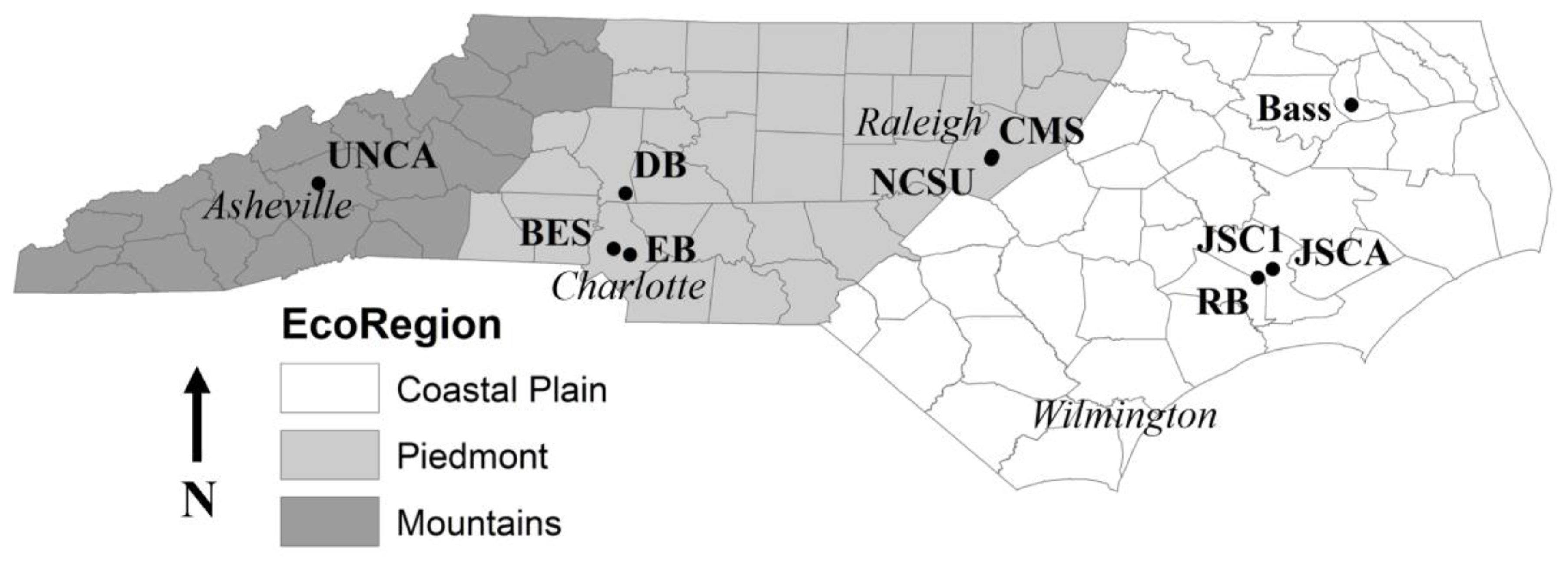
Locations of CSWs studied within the state of North Carolina.

Figure 2.
Example model calibration (a) and validation (b) results: observed vs. predicted TN effluent concentrations from the RB CSW with resultant statistical indices: R2, NSE, and RMSE.
Figure 2.
Example model calibration (a) and validation (b) results: observed vs. predicted TN effluent concentrations from the RB CSW with resultant statistical indices: R2, NSE, and RMSE.

Figure 3.
Observed vs. model predicted plots from calibration exercises for: (a) TN; (b) TAN; (c) NO2,3-N; (d) ON; (e) TP; and (f) TSS.
Figure 3.
Observed vs. model predicted plots from calibration exercises for: (a) TN; (b) TAN; (c) NO2,3-N; (d) ON; (e) TP; and (f) TSS.
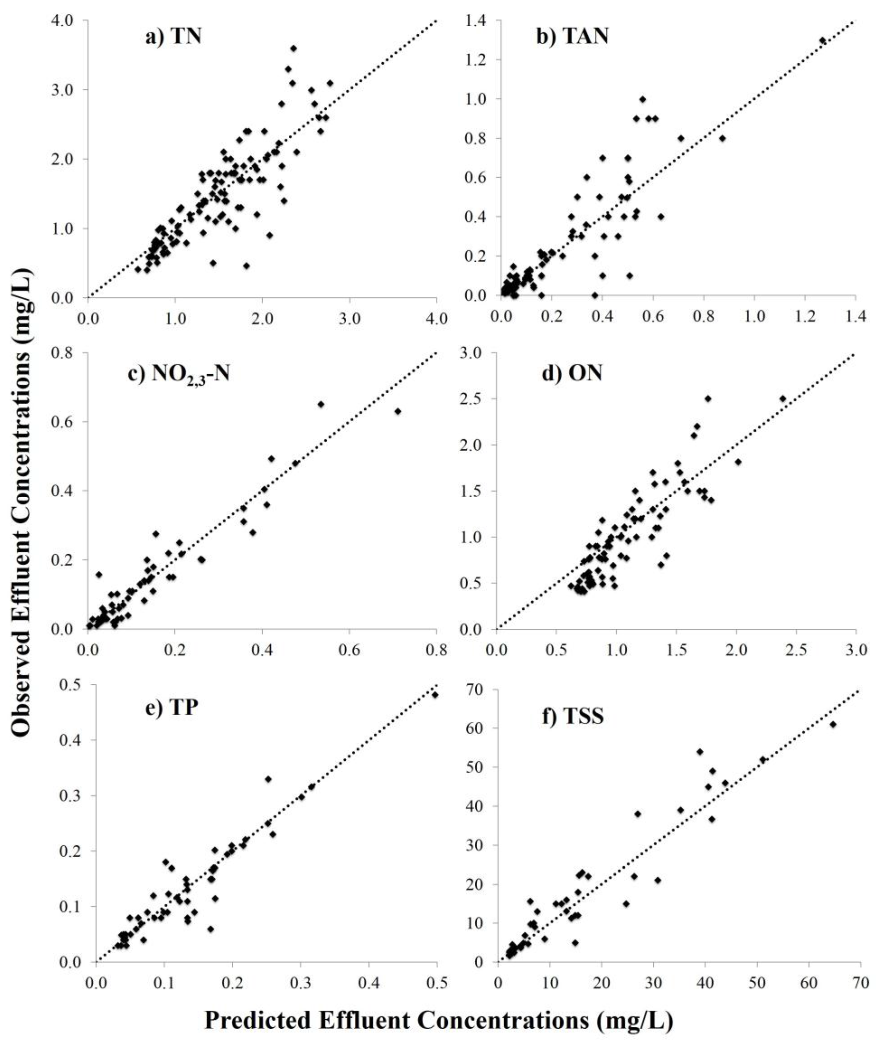
Figure 4.
Observed vs. model predicted plots from validation for: (a) TN; (b) TAN; (c) NO2,3-N; (d) ON; (e) TP; and (f) TSS.
Figure 4.
Observed vs. model predicted plots from validation for: (a) TN; (b) TAN; (c) NO2,3-N; (d) ON; (e) TP; and (f) TSS.

Figure 5.
Distributions for each of the three model parameters (P, θ, and k20) for all CSW sites and all pollutants according to the sensitivity analysis. The scale of the y-axis is presented as a percentage of the total number of accepted (NSE > 0) parameter sets.
Figure 5.
Distributions for each of the three model parameters (P, θ, and k20) for all CSW sites and all pollutants according to the sensitivity analysis. The scale of the y-axis is presented as a percentage of the total number of accepted (NSE > 0) parameter sets.


Table 1.
Percent Concentration Reduction and Mean Effluent Concentrations (mg/L) for Six CSWs Studied in North Carolina.
Table 1.
Percent Concentration Reduction and Mean Effluent Concentrations (mg/L) for Six CSWs Studied in North Carolina.
| Study | Location | Contributing Watershed 1 | TN | TP | TSS |
|---|---|---|---|---|---|
| Bass, 2000 [10] | Edenton | U, A | 20% (2.10) | −55% (0.57) | - |
| Johnson, 2006 [11] | Charlotte | U | 40% (1.40) | 55% (0.20) | 66% (24) |
| Line et al., 2008 [12] | Asheville | U | 42% (0.94) | 52% (0.12) | 83% (31) |
| Line et al., 2008 [12] | Raleigh | U, GC | 21% (1.00) | 43% (0.99) | 64% (28) |
| Hathaway and Hunt, 2010 [2] 2 | Mooresville | U | 52% (0.84) | 61% (0.12) | 84% (12) |
| Merriman and Hunt, 2014 [9] | River Bend | U, GC | 1% (0.86) | 8% (0.19) | 15% (8.4) |
| CSW Assigned Removal Credits 3: | 40% | 40% | 85% | ||
| CSW Target Effluent Concentrations (mg/L) 4: | 1.08 | 0.12 | 25 | ||
Table 2.
Physical characteristics of CSWs and their watersheds.
| Wetland Name | Reference | Wetland and Watershed Characteristics | |||||
|---|---|---|---|---|---|---|---|
| Age when Studied (years) | Wetland Area (ha) | Watershed Curve Number | Watershed Area (ha) | Monitoring Period | Events | ||
| Bass | [10] | 1–2 | 1 | 75 | 240 | January 1996–December 1999 | 116 |
| Bruns Elementary (BES) | [11] | 2 | 0.13 | 85 | 6.4 | March–September 2006 | 15 |
| Edward’s Branch (EB) | [30] | 4 | 0.2 | 83 | 36.4 | April 2004–December 2005 | 16 |
| North Carolina State University (NCSU) | [31] | 1 | 0.03 | 77 | 4.2 | March–June 2007 | 12 |
| Centennial Middle School (CMS) | [12] | 4 | 0.2 | 73 | 9.6 | April–August 2006 | 5 |
| University of North Carolina—Asheville (UNCA) | [12] | 4 | 0.07 | 76 | 4.1 | April–August 2006 | 11 |
| Dye Branch: Cell 1 (DB) | [2] | 2 | 0.33 | 88 | 12.5 | February–October 2008 | 16 |
| River Bend (RB) | [9] | 5 | 0.14 | 54 | 46.5 | March 2012–May 2013 | 16 |
| Jack Smith Creek: Cell 1 (JSC1) | [8] | 1 | 1.67 | 82 | 620 | June 2013–October 2014 | 27 |
| Jack Smith Creek: Cell A (JSCA) | [8] | 1 | 1.45 | 82 | 620 | June 2013–October 2014 | 23 |
Table 3.
Observed inlet and outlet EMC medians and standard deviations, in parenthesis, (mg/L) for each CSW and number of events for each pollutant.
Table 3.
Observed inlet and outlet EMC medians and standard deviations, in parenthesis, (mg/L) for each CSW and number of events for each pollutant.
| CSW | Inlet vs. Outlet | NO2,3-N a | TAN b | ON c | TN d | TP e | TSS f |
|---|---|---|---|---|---|---|---|
| Bass | Inlet | 0.50 (0.40) | 0.50 (0.49) | 1.46 (0.60) | 2.69 (0.80) | 0.31 (0.20) | 19.9 (23.3) |
| Outlet | 0.10 (0.36) | 0.40 (0.38) | 1.40 (0.60) | 2.00 (0.80) | 0.48 (0.34) | 14.0 (17.4) | |
| BES | Inlet | 0.69 (0.27) | 0.24 (0.32) | 1.25 (0.46) | 2.02 (0.96) | 0.32 (0.40) | 67.9 (40.5) |
| Outlet | 0.50 (0.16) | 0.10 (0.06) | 0.76 (0.21) | 1.37 (0.37) | 0.17 (0.12) | 21.0 (13.8) | |
| EB | Inlet | 0.47 (0.20) | 0.15 (0.41) | 0.90 (0.80) | 1.76 (1.30) | 0.19 (0.12) | 24.0 (17.0) |
| Outlet | 0.14 (0.11) | 0.10 (0.11) | 0.81 (0.28) | 1.05 (0.40) | 0.09 (0.09) | 21.5 (17.8) | |
| NCSU | Inlet | 0.51 (0.30) | 0.56 (0.34) | 1.65 (1.21) | 2.45 (1.70) | 0.30 (0.16) | 155 (167) |
| Outlet | 0.31 (0.13) | 0.33 (0.16) | 1.30 (0.70) | 2.06 (0.86) | 0.20 (0.11) | 82.0 (128) | |
| CMS | Inlet | 0.22 (0.10) | 0.12 (0.27) | 0.58 (0.35) | 0.90 (0.60) | 0.17 (0.22) | 20.0 (63.0) |
| Outlet | 0.15 (0.18) | 0.18 (0.18) | 0.80 (0.33) | 1.22 (0.59) | 0.18 (0.06) | 38.0 (21.7) | |
| UNCA | Inlet | 0.34 (0.28) | 0.22 (0.32) | 1.74 (0.56) | 2.47 (0.91) | 0.38 (0.25) | 352 (110) |
| Outlet | 0.15 (0.15) | 0.08 (0.15) | 0.74 (1.00) | 0.94 (1.10) | 0.12 (0.21) | 31.3 (54.3) | |
| DB | Inlet | 0.40 (0.16) | 0.21 (0.25) | 0.96 (0.31) | 1.65 (0.55) | 0.26 (0.25) | 79.0 (40.4) |
| Outlet | 0.14 (0.12) | 0.02 (0.03) | 0.70 (0.18) | 0.86 (0.19) | 0.11 (0.05) | 12.0 (4.46) | |
| RB | Inlet | 0.10 (0.09) | 0.06 (0.07 | 0.63 (0.26) | 0.74 (0.32) | 0.17 (0.11) | 7.61 (7.61) |
| Outlet | 0.03 (0.07) | 0.04 (0.06) | 0.70 (0.25) | 0.83 (0.29 | 0.20 (0.06) | 7.95 (3.43) | |
| JSC1 | Inlet | 0.16 (0.22) | 0.07 (0.14) | 0.94 (0.46) | 1.38 (0.59) | 0.21 (0.11) | 30.5 (32.1) |
| Outlet | 0.05 (0.06) | 0.06 (0.11) | 0.52 (0.21) | 0.68 (0.28) | 0.05 (0.03) | 3.35 (5.03) | |
| JSCA | Inlet | 0.14 (0.08) | 0.09 (0.06) | 1.02 (0.69) | 1.25 (0.70) | 0.28 (0.19) | 49.9 (51.8) |
| Outlet | 0.04 (0.03) | 0.03 (0.02) | 0.49 (0.14) | 0.56 (0.14) | 0.06 (0.02) | 3.64 (2.56) | |
| Total Number of Events: | 108 | 160 | 148 | 205 | 100 | 82 | |
Table 4.
CSW design characteristics.
| CSW | Free Water Depth, h (cm) | Detention Time, τ (days) |
|---|---|---|
| Bass | 30 | 1.5 |
| BES | 20 | 2 |
| EB | 30 | 2 |
| NCSU | 23 | 0.5 |
| CMS | 30 | 2 |
| UNCA | 10 | 0.1 |
| DB | 30 | 3 |
| RB | 25 | 2 |
| JSC1 | 20 | 2 |
| JSCA | 30 | 1 |
Table 5.
Model fit parameters P, θ, and k20 (m/year) for each pollutant observed in individual CSWs.
Table 5.
Model fit parameters P, θ, and k20 (m/year) for each pollutant observed in individual CSWs.
| CSW | TN | TAN | NO2,3-N | ON | TP | TSS | ||||||||||||
|---|---|---|---|---|---|---|---|---|---|---|---|---|---|---|---|---|---|---|
| P | θ | k20 | P | θ | k20 | P | θ | k20 | P | θ | k20 | P | θ | k20 | P | θ | k20 | |
| BES | 5.4 | 1.029 | 38.7 | 3.9 | 0.979 | 12.7 | 3.0 | 1.008 | 10.9 | 3.0 | 1.104 | 57.8 | 2.7 | 1.007 | 14.0 | 3.6 | 1.005 | 24.8 |
| RB | 3.0 | 1.023 | 5.1 | 3.0 | 0.981 | 13.5 | 7.3 | 0.954 | 22.2 | - | - | - | 4.8 | 0.918 | 4.4 | 3.0 | 0.951 | 10.4 |
| CMS | 2.7 | 1.020 | 61.6 | 3.0 | 1.016 | 40.3 | 4.0 | 0.991 | 24.9 | - | - | - | 6.4 | 0.882 | 58.3 | 7.6 | 0.974 | 84.0 |
| UNCA | 1.7 | 0.968 | 46.1 | 3.0 | 1.018 | 75.6 | 6.1 | 1.106 | 85.5 | 4.0 | 1.019 | 67.0 | 3.0 | 1.191 | 37.0 | 5.0 | 1.077 | 170.8 |
| NCSU | 3.0 | 1.108 | 52.6 | 2.9 | 0.965 | 39.2 | 4.0 | 0.982 | 73.8 | 3.2 | 0.934 | 140.8 | 3.8 | 1.043 | 53.5 | 1.6 | 1.034 | 183.3 |
| EB | 1.7 | 0.948 | 44.3 | 4.0 | 0.953 | 33.1 | 3.0 | 0.975 | 39.1 | 1.4 | 0.929 | 76.4 | 1.8 | 0.973 | 37.1 | 4.0 | 1.009 | 15.3 |
| DB | 2.1 | 0.965 | 63.1 | 3.2 | 1.047 | 65.4 | 3.0 | 1.073 | 50.4 | 5.0 | 1.286 | 40.5 | 4.5 | 1.027 | 18.0 | 2.4 | 0.985 | 84.0 |
| JSC1 | 3.3 | 0.994 | 57.3 | 3.0 | 1.041 | 23.6 | 1.5 | 1.107 | 31.9 | 3.0 | 1.050 | 30.2 | 3.9 | 1.028 | 35.7 | 1.8 | 0.990 | 164.0 |
| JSCA | - | - | - | - | - | - | 4.5 | 1.019 | 250.9 | 3.6 | 0.960 | 161.0 | 2.9 | 0.954 | 84.2 | 2.9 | 0.914 | 421.1 |
| Bass | 4.1 | 1.006 | 28.7 | 3.0 | 1.017 | 34.2 | - | - | - | 4.9 | 0.986 | 28.2 | - | - | - | - | - | - |
| Mean | 3.0 | 1.007 | 44.2 | 3.2 | 1.002 | 37.5 | 4.0 | 1.024 | 65.5 | 3.5 | 1.034 | 75.2 | 3.7 | 1.002 | 38.0 | 3.6 | 0.993 | 128.6 |
| Median | 3.0 | 1.006 | 46.1 | 3.0 | 1.016 | 34.2 | 4.0 | 1.008 | 39.1 | 3.4 | 1.003 | 62.4 | 3.8 | 1.007 | 37.0 | 3.0 | 0.990 | 84.0 |
Table 6.
Mean CSW removal rate constants for each pollutant and respected percentile in the distribution of rate constants compiled by Kadlec and Wallace (2008) [3].
Table 6.
Mean CSW removal rate constants for each pollutant and respected percentile in the distribution of rate constants compiled by Kadlec and Wallace (2008) [3].
| Pollutant | Mean (m/year) | Treatment Wetlands Percentile |
|---|---|---|
| TN | 44.2 | 91% |
| TAN | 37.5 | 66% |
| NO2,3-N | 65.5 | 91% |
| ON | 75.2 | 91% |
| TP | 38.0 | 84% |
| TSS | 128.6 | - |
Table 7.
Calibration Statistical Evaluations: RMSE (mg/L), R2, and NSE.
| TN | TAN | NO2,3-N | ON | TP | TSS | |||||||||||||
|---|---|---|---|---|---|---|---|---|---|---|---|---|---|---|---|---|---|---|
| CSW | RMSE | R2 | NSE | RMSE | R2 | NSE | RMSE | R2 | NSE | RMSE | R2 | NSE | RMSE | R2 | NSE | RMSE | R2 | NSE |
| BES | 0.16 | 0.55 | 0.54 | 0.04 | 0.61 | 0.60 | 0.07 | 0.75 | 0.73 | 0.10 | 0.64 | 0.63 | 0.05 | 0.67 | 0.54 | 6.33 | 0.84 | 0.84 |
| RB | 0.14 | 0.97 | 0.85 | 0.00 | 0.97 | 0.95 | 0.03 | 0.71 | 0.69 | - | - | - | 0.01 | 0.92 | 0.92 | 1.16 | 0.90 | 0.89 |
| CMS | 0.02 | 1.00 | 1.00 | 0.03 | 0.98 | 0.98 | 0.03 | 0.71 | 0.68 | - | - | - | 0.00 | 1.00 | 1.00 | 6.82 | 0.94 | 0.90 |
| UNCA | 0.29 | 0.57 | 0.51 | 0.05 | 0.42 | 0.28 | 0.09 | 0.41 | 0.19 | 0.21 | 0.50 | 0.42 | 0.05 | 0.66 | 0.63 | 6.37 | 0.82 | 0.56 |
| NCSU | 0.42 | 0.65 | −0.73 | 0.06 | 0.83 | 0.79 | 0.05 | 0.93 | 0.76 | 0.16 | 0.83 | 0.79 | 0.02 | 1.00 | 0.98 | 31.48 | 0.74 | 0.72 |
| EB | 0.11 | 0.91 | 0.93 | 0.05 | 0.79 | 0.77 | 0.03 | 0.65 | 0.60 | 0.18 | 0.95 | 0.62 | 0.01 | 0.88 | 0.84 | 4.93 | 0.84 | 0.84 |
| DB | 0.16 | 0.45 | 0.39 | 0.02 | 0.79 | 0.78 | 0.04 | 0.63 | 0.61 | 0.17 | 0.53 | 0.30 | 0.04 | 0.52 | 0.48 | 3.29 | 0.26 | −1.47 |
| JSC1 | 0.15 | 0.68 | 0.31 | 0.01 | 0.95 | 0.83 | 0.02 | 0.94 | 0.93 | 0.00 | 0.45 | 0.43 | 0.00 | 0.78 | 0.74 | 0.48 | 0.71 | 0.45 |
| JSCA | - | - | - | - | - | - | 0.01 | 0.63 | 0.63 | 0.08 | 0.70 | 0.49 | 0.02 | 0.28 | 0.23 | 0.80 | 0.48 | 0.40 |
| Bass | 0.48 | 0.43 | 0.43 | 0.20 | 0.62 | 0.62 | - | - | - | 0.31 | 0.58 | 0.58 | - | - | - | - | - | - |
| Mean | 0.21 | 0.69 | 0.47 | 0.05 | 0.77 | 0.73 | 0.04 | 0.71 | 0.65 | 0.15 | 0.65 | 0.53 | 0.02 | 0.75 | 0.71 | 6.85 | 0.72 | 0.46 |
| Median | 0.16 | 0.65 | 0.51 | 0.04 | 0.79 | 0.78 | 0.03 | 0.71 | 0.68 | 0.16 | 0.61 | 0.53 | 0.02 | 0.78 | 0.74 | 4.93 | 0.82 | 0.72 |
Table 8.
Validation Statistical Evaluations: RMSE (mg/L), R2, and NSE.
| TN | TAN | NO2,3-N | ON | TP | TSS | |||||||||||||
|---|---|---|---|---|---|---|---|---|---|---|---|---|---|---|---|---|---|---|
| CSW | RMSE | R2 | NSE | RMSE | R2 | NSE | RMSE | R2 | NSE | RMSE | R2 | NSE | RMSE | R2 | NSE | RMSE | R2 | NSE |
| BES | 0.17 | 0.00 | −0.15 | 0.21 | 0.88 | −8.33 | 0.16 | 0.70 | 0.63 | 0.28 | 0.17 | −0.33 | 0.04 | 0.41 | 0.38 | 9.03 | 0.49 | 0.22 |
| RB | 0.17 | 0.67 | 0.16 | 0.05 | 0.70 | −0.71 | 0.04 | 0.85 | 0.83 | - | - | - | 0.02 | 0.96 | 0.92 | 0.74 | 0.94 | 0.89 |
| CMS | - | - | - | - | - | - | - | - | - | - | - | - | - | - | - | - | - | - |
| UNCA | - | - | - | 0.05 | 0.42 | −0.31 | 0.03 | 0.98 | 0.72 | - | - | - | 0.08 | 0.85 | 0.80 | 14.28 | 0.26 | −0.36 |
| NCSU | - | - | - | 0.07 | 0.86 | 0.84 | 0.05 | 0.91 | 0.91 | - | - | - | 0.09 | 0.26 | −0.35 | 124.36 | 0.98 | 0.52 |
| EB | 0.16 | 0.81 | 0.53 | - | - | - | 0.05 | 0.86 | 0.42 | 0.22 | 0.31 | 0.06 | 0.03 | 0.56 | 0.30 | 15.47 | 0.26 | −7.99 |
| DB | 0.10 | 0.07 | −2.41 | 0.02 | 0.59 | 0.54 | 0.10 | 0.02 | −1.12 | 0.46 | 0.90 | −21.77 | 0.05 | 0.15 | −1.03 | 4.16 | 0.37 | −0.39 |
| JSC1 | 0.20 | 0.00 | −0.51 | 0.01 | 0.92 | 0.45 | 0.03 | 0.84 | 0.59 | 0.15 | 0.01 | −0.08 | 0.01 | 0.52 | 0.24 | 0.85 | 0.88 | 0.14 |
| JSCA | - | - | - | - | - | - | 0.02 | 0.97 | −0.47 | 0.14 | 0.03 | −4.42 | 0.02 | 0.72 | 0.52 | 0.61 | 0.90 | 0.59 |
| Bass | 0.40 | 0.52 | 0.51 | 0.22 | 0.67 | 0.67 | - | - | - | 0.28 | 0.65 | 0.65 | - | - | - | - | - | - |
| Mean | 0.20 | 0.34 | −0.31 | 0.09 | 0.72 | −0.98 | 0.06 | 0.77 | 0.31 | 0.25 | 0.34 | −4.32 | 0.04 | 0.56 | 0.22 | 21.19 | 0.64 | −0.80 |
| Median | 0.17 | 0.29 | 0.00 | 0.05 | 0.70 | 0.45 | 0.04 | 0.86 | 0.61 | 0.25 | 0.24 | −0.21 | 0.03 | 0.54 | 0.34 | 6.59 | 0.68 | 0.18 |
Table 9.
Statistical metrics for pollutants observed in NC CSW studies.
| Pollutant | Calibration | Validation | ||||
|---|---|---|---|---|---|---|
| n | RMSE (mg/L) | NSE | n | RMSE (mg/L) | NSE | |
| TN | 115 | 0.37 | 0.72 | 90 | 0.33 | 0.78 |
| TAN | 86 | 0.13 | 0.78 | 74 | 0.17 | 0.74 |
| NO2,3-N | 57 | 0.05 | 0.91 | 51 | 0.07 | 0.87 |
| ON | 82 | 0.26 | 0.72 | 66 | 0.31 | 0.62 |
| TP | 51 | 0.03 | 0.88 | 49 | 0.05 | 0.73 |
| TSS | 45 | 5.01 | 0.91 | 37 | 9.30 | 0.63 |
© 2017 by the authors. Licensee MDPI, Basel, Switzerland. This article is an open access article distributed under the terms and conditions of the Creative Commons Attribution (CC BY) license (http://creativecommons.org/licenses/by/4.0/).
Share and Cite
MDPI and ACS Style
Merriman, L.S.; Hathaway, J.M.; Burchell, M.R.; Hunt, W.F. Adapting the Relaxed Tanks-in-Series Model for Stormwater Wetland Water Quality Performance. Water 2017, 9, 691. https://doi.org/10.3390/w9090691
AMA Style
Merriman LS, Hathaway JM, Burchell MR, Hunt WF. Adapting the Relaxed Tanks-in-Series Model for Stormwater Wetland Water Quality Performance. Water. 2017; 9(9):691. https://doi.org/10.3390/w9090691
Chicago/Turabian StyleMerriman, Laura S., Jon M. Hathaway, Michael R. Burchell, and William F. Hunt. 2017. "Adapting the Relaxed Tanks-in-Series Model for Stormwater Wetland Water Quality Performance" Water 9, no. 9: 691. https://doi.org/10.3390/w9090691
Note that from the first issue of 2016, this journal uses article numbers instead of page numbers. See further details here.