Optimization of a Water Quality Monitoring Network Using a Spatially Referenced Water Quality Model and a Genetic Algorithm


Biological and Agricultural Engineering Department, Texas A & M University, 2117 TAMU, College Station, TX 77843, USA
*
Author to whom correspondence should be addressed.
Water 2017, 9(9), 704; https://doi.org/10.3390/w9090704
Submission received: 14 June 2017
/
Revised: 25 August 2017
/
Accepted: 12 September 2017
/
Published: 15 September 2017
Abstract
:The monitoring network for a river system is designed to provide information about water quantity and quality. The development of Watershed Protection Plans and Total Maximum Daily Loads require systematic monitoring of waterbodies. In this study, optimum water quality monitoring networks were selected to assess E. coli loads in the Guadalupe River and San Antonio River basins. A Genetic Algorithm (GA) was applied to select monitoring stations using the mean annual E. coli flux from the Spatially Referenced Regression Model on Watershed Attributes (SPARROW). The objectives of the GA were to minimize the number of monitoring stations, include large values of the mean annual E. coli flux, and minimize uncertainty of the flux estimations. Constraints related to the monitoring of critical locations were included in a multi-objective optimization problem. The SPARROW model was applied to the optimized GA solution sets, which were compared using the objective values and statistical indices. The best GA-generated alternative set adequately represented the San Antonio River basin, in good agreement with a previous study conducted using only SPARROW. The application of the GA ensured the inclusion of the monitoring stations with large values of E. coli flux, which reflected high-risk areas within the watershed.
1. Introduction
The monitoring network for a river system is designed to provide information about water quantity and quality. The water-quality monitoring stations are located at critical locations for the surveillance of waterbodies from pollution sources. Water resources utility and management programs such as Total Maximum Daily Loads (TMDL) development and Watershed Protection Plans (WPP) also require the systematic monitoring of waterbodies [1]. To design a water quality monitoring network, the contaminant sources and the respective loads must be considered. To reduce the contaminant load from point and nonpoint sources being delivered to streams, the development of TMDLs requires a reasonable assessment of those sources. The monitoring network may be subjected to objectives and constraints related to the cost of monitoring and trends of regional water quality [2]. Identifying the optimal locations could not only reduce costs, but also provide a better representation of a watershed. Optimization of the monitoring network can enable watershed managers to prioritize specific objectives to design a more effective monitoring network.
Genetic Algorithm (GA) is an optimization approach based on Darwin’s evolution concept of natural selection [3]. GA is a robust technique to obtain near-optimal solutions in the decision space by a randomly-chosen initial solution set. The solution space is explored and exploited by applying genetic operators such as crossover, mutation, and selection methods. For water quality research, GAs have been used to calibrate and perform sensitivity analysis on models and to allocate the contaminant load with uncertainty [4,5,6]. Icaga [7] compared the results of a GA to a previous application of dynamic programming for reducing the number of monitoring stations in a basin. It was observed that the performance of a GA, which varies greatly, depends on the initial population size, crossover and mutation rates. Park et al. [1] applied a single objective GA by aggregating multiple objectives with normalized weights based on the River Basin representation, water-quality standard compliances, and pollution sources supervision. They found that the existing monitoring-network design required significant improvements for converting it into an optimum network. Reed et al. [8] discussed practical methodologies to implement an efficient single objective GA to design a groundwater quality monitoring network. They further explored the application of multi-objective algorithm to minimize the cost and error in estimation of concentration of contaminants by reducing the number of groundwater monitoring stations [9].
The previously mentioned studies were implemented to design monitoring networks or allocate loads for non-pathogenic contaminants. Bacteria contamination has become a dominant water quality issue in the U.S. in recent years, largely because of increasing population, failing septic systems, and non-point pollution (from forests, pasture land uses and urban land uses) [10]. There are only limited water-quality records available for bacteria compared to traditionally observed water quality parameters such as nutrients. Modeling approaches to develop TMDLs, using the monitored water-quality data as input, are widely used to assess the bacteria load from non-point and point sources. Because monitoring data are scarce, uncertainty increases for the bacterial load assessment [11]. Therefore, to optimize performance of a water-quality model, uncertainty in the monitored records should be minimized.
The Spatially Referenced Regression Model on Watershed Attributes (SPARROW) is a water quality model that predicts fluxes and concentrations and tracks the sources of the contaminants [12,13,14]. Using simple empirical relationships, SPARROW can be applied in lieu of complex mechanistic models, especially when water quality data are limited. The SPARROW model relates the monitored water quality records to spatially-referenced contaminant sources and land–water delivery factors within the stream or watershed. These factors can affect the increase, decay, and delivery of a bacteria load in a stream network. E. coli concentrations are often monitored monthly or randomly, such as during or after storm events. To estimate the mean annual E. coli flux, the concentrations are analyzed with daily streamflow records by applying a load-estimator model (FLUXMASTER). The mean annual fluxes of the water-quality monitoring stations serve as the response variables for SPARROW. A simplified flowchart description of the SPARROW model, integrated with FLUXMASTER, is detailed elsewhere [13].
Smith et al. [14] recommended using SPARROW to design a monitoring network by considering the prediction improvement when simulating for different sampling locations. However, monitoring limitations create uncertainty in the mean annual flux estimations, which can produce large errors in SPARROW predictions. These limitations include scarcity of monitored data, location of monitoring stations, and irregular monitoring intervals. An optimum set of monitoring stations can be selected from the existing monitoring network based on a simple application of SPARROW, as previously studied [13].
In this study, the optimum water quality monitoring networks were selected to assess E. coli loads with minimal uncertainty for two major river basins (Guadalupe River and San Antonio River) of Texas. A GA was applied to select the monitoring networks with adequate spatial variation from the FLUXMASTER assessment of mean annual flux. The objectives of the GA application were: (1) to minimize the number of monitoring stations; (2) to include large values of mean annual flux; and (3) to minimize the uncertainty with regard to flux estimations. Constraints related to the monitoring of critical locations were included in a multi-objective optimization problem. The SPARROW model was then applied to the GA solution sets. From the optimum sets of monitoring stations, the best monitoring network was selected based on the objective values and statistical indices. Performance of the “optimized” network was then compared to a previous model that was selected only using SPARROW.
2. Methodology
2.1. Study Area and Data Sources
The SPARROW model was applied to assess E. coli flux, an indicator of fecal contamination, in the Guadalupe and San Antonio River Basins of Texas. The spatial extent of the study area (area 29,380 km2) is from longitude 30°18′44″ N to 28°22′2″ S and from latitude 99°42′31″ W to 96°47′10″ E. The study area includes a metropolitan area (San Antonio), an unconfined aquifer (Edwards Aquifer), and forest and pasture as major land uses (55.4% and 28.0%, respectively). Attributes such as land use, average temperature and precipitation, reach slope and velocity, and reservoir area were obtained from the National Hydrography Dataset (NHD) Plus [15]. Monitored records of E. coli concentrations were obtained from the Guadalupe Blanco River Authority (GBRA) and San Antonio River Authority (SARA) [16,17]. The daily stream-flow data at stream gauges were available from United State Geological Survey (USGS) [18]. The effluent discharge [19] from wastewater treatment plants (WWTPs) were included as probable E. coli sources. Because the concentration data of contaminants in the effluent was not available, the permitted flows from WWTPs were used in the model. There were many point sources throughout the study area that discharged relatively low flows; therefore, only the WWTPs with discharge greater than two million gallons per day were included. Low discharging WWTPs were not used in the model to ensure that large mean annual E. coli fluxes were included Soil permeability values were derived from the State Soil Geographic Database (STATSGO) [20]. In SPARROW, the reach length and depth reflect temporal changes and sunlight penetration, which affect the decay of bacteria. Further, the streams were divided into three categories (small, medium and large) on a quantile basis for the reach decay factors. Figure 1 shows the location of the monitoring stations in the Guadalupe and San Antonio sub-basins. Reaches with flow greater than 0.13 m3 s−1 are defined as major streams.
To reduce the effect of irregular monitoring and the short time period of records on the water quality assessment, an initial set of monitoring stations was selected on the basis of standard error to mean annual flux ratio in FLUXMASTER. Only 56 out of 72 monitoring stations were selected as inputs for the GA, mainly because of the availability of E. coli data; stations without regular monitoring were excluded. Additionally, to minimize uncertainty, only stations with at least a two-year duration and 10 observations were considered. Schwarz et al. [21] recommended at least 20 monitoring stations for the application of SPARROW to include the spatial variability. The model error in the SPARROW predictions is related to the quality and scale of explanatory variables. Applying combinatorial mathematics, there are 7.86 × 10¹⁴ possibilities to select 20 stations from the 56 monitoring stations with equal probability.
2.2. Genetic Algorithm Overview
To initialize the GA, a random set (called the population) of solutions were coded into various formats, such as binary, real, integers, etc. These solutions are called chromosomes. Every chromosome consists of genes that provide information on the solution attributes. The population of solutions was evaluated for fitness. The fitness value indicated how well a solution met the problem’s objective functions and constraints. The variation operators, mutation and recombination, were applied to create a diverse set of new solutions (called children) from the existing solutions (called parents). Recombination or crossover includes the interaction between two or more parents, whereas mutation is the outcome of a random change in the chromosome of a parent. The children were tested for their fitness, and then selected as parents in a new generation. The mutation operator explored new solutions from unexplored regions in the solution space. The selection operation ensured overall improvement in the mean quality of solutions in the next generation. The newly created generation was treated as parents until either the solution set converged to the best possible solution or a predefined termination condition was met [22].
To efficiently obtain the optimal solution, the application of a GA also includes decision making to select the parameters for the genetic operations [23]. To solve a multi-objective problem, two different strategies can be applied either by aggregating the weighted objectives to form a single objective problem or by finding the multiple solutions on a Pareto front to generate the best alternatives. The first method provides the leverage to solve the problem as a single objective, but assigning weights can be challenging for most problems. The second method requires solving the problem for all the objectives to obtain the non-dominated or Pareto set of solutions. Non-dominated sets of solutions consist of feasible optimal solutions. Non-dominated solutions sacrifice in one objective(s) to achieve gain in the other objective(s) of a problem. This provides the flexibility of different possible options to make a final decision. The dimension of Pareto front is equal to the number of objectives in the problem. It is desired that the Pareto front should provide the uniformly distributed and complete spectrum of the problem including the extreme ends of the objective functions. Based on the second method, various multi-objective algorithms such as Vector Evaluated Genetic Algorithm (VEGA), Strength Pareto Evolutionary Algorithm (SPEA), Non-dominated Sorted Genetic Algorithm (NSGA) and their modifications are available [24,25]. These algorithms are designed on the basis of dominance rank, count, distance, or their combination to distinguish between the dominated and non-dominated solutions. A member’s dominance rank and count are defined on the basis of the number of members dominating the member and the number of members being dominated by the member. The distance is a measure of the well distributed Pareto front. In this study, a GA based on the Multi-Objective Evolutionary Algorithm (MOEA) [26] was used to obtain the Pareto sets for the optimized monitoring network.
2.3. Objectives and Constraints
Uncertainty in prediction of mean annual flux by regressions tools, such as FLUXMASTER, can occur due to poor data quality and quantity. To minimize the effect of the uncertainty in FLUXMASTER on SPARROW predictions, uncertainty was considered a selection objective. A solution was represented by a binary string of 56 genes: 0 for “not selected” and 1 for “selected”. The objectives were defined mathematically for the GA application:
1. To minimize cost, the number of monitoring stations was kept as small as possible without compromising the water quality standard. As such, maintaining longer duration records for a smaller, but sufficient number of monitoring stations is preferable to collecting many redundant monitoring records of shorter duration,
where is the decision to include a monitoring station at location i.
2. The average of the logarithm of the mean annual fluxes for all the monitoring stations was maximized to ensure that stations selected for model calibration included high risk areas,
where mi is the predicted mean annual flux from the FLUXMASTER output.
3. The standard error to flux ratio for the monitoring stations was minimized to mitigate bias associated with large standard errors of the mean annual flux [27],
where SFi is the standard error to mean annual flux ratio.
The constraints were defined to find the optimal solutions with the GA:
1. To represent sufficient spatial variability of the water quality in the region, the total number of monitoring stations was greater than 20.
2. Monitoring station locations with ecological or hydrological importance, which require continuous monitoring, must remain in the network. In this study, the Edwards Aquifer contributing zone, with four monitoring stations, has an impact on the recharge of the aquifer. Likewise, the City of San Antonio has six monitoring stations. To account for the importance of these two areas, at least two stations in the Edwards Aquifer region and three stations in San Antonio were retained in the final solution. If a set of monitoring stations violated this constraint, a penalty was imposed by making the value of the third objective impossibly large.
2.4. GA Application
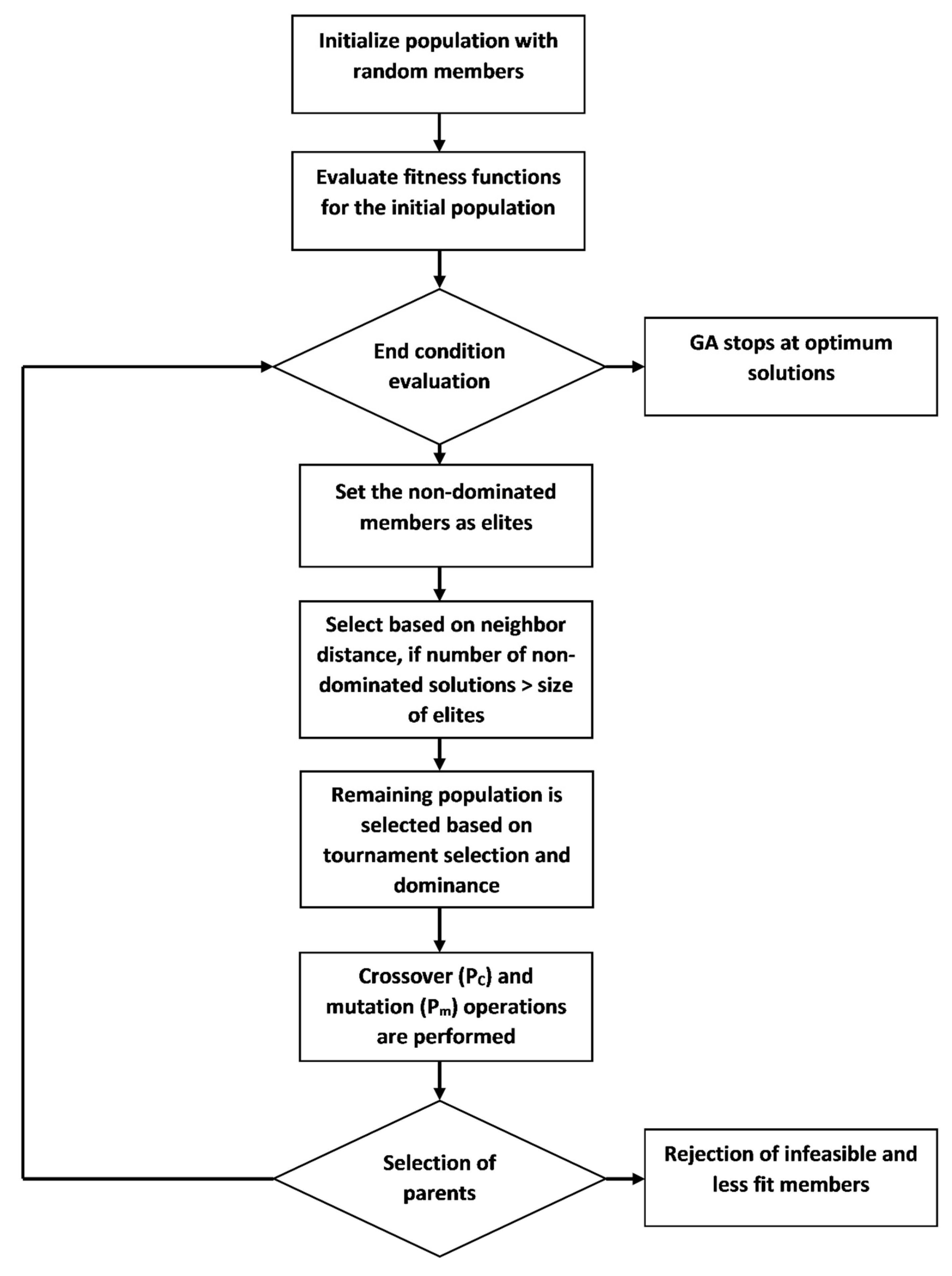
The population size of 100 was selected for this application of a GA. After trying different numbers of generations for the convergence of the population, the number of generations was kept as 30. The size of the elite set, members of a population which go directly to the next generation, was 20. Two-point binary crossover with a probability (PC) of 0.6 was used, whereas mutation (Pm) was uniformly distributed with the probability of 0.05. In the two-point crossover operator, two positions in the parents’ strings were chosen at random; new offspring were formed by swapping the element values between parents. When applied, the uniformly distributed operator chose an element in the original member and that element was changed to a random value between the defined upper and lower bounds. Using the modified MOEA (Figure 2), the non-dominated solutions from every generation entered as elites. The remaining population was chosen from among the dominated solutions, using tournament selection, by comparing all the objectives for optimal values (higher value of Objective 2 and lower values of Objective 1 and Objective 3). Elites went directly to the next generation, while the other solutions went through crossover and mutation operators. If there were more non-dominated solutions than elites, then the elites were selected based on the neighborhood distance:
where D(x), the neighborhood distance for a member x, is the sum of the distances from m nearest solutions on the same Pareto front; and nd is the number of non-dominated members.
In this problem, m was equal to three. The process continued until the last generation. The GA was repeated ten times to compare the results. Finally, the SPARROW model was applied on the Pareto solutions.
2.5. Statistical Indices
After applying SPARROW to the optimum sets of monitoring stations, several indices were used to evaluate the respective models. Because SPARROW is a regression model, the coefficient of determination (R2) and the root mean of the square of the errors (RMSE) were used to assess the goodness of fit for each model. Ideally, the RMSE of the annual mean E. coli fluxes for a set of monitoring stations would be minimized and the R2 would approach 1. However, each model incorporated different parameters and number of observations. Therefore, additional criteria were used to compare the model performance.
To gauge complexity and accuracy, the Akaike Information Criterion (AIC) was calculated. A lower AIC, which would indicate a less complex model with minimal error, was desired. The Nash–Sutcliffe Efficiency (NSE) reflects agreement between observed and predicted values; NSE values range from −∞ to 1 [28]. Negative NSE values indicate a biased model, whereas unbiased agreement increases as the values approach unity. The tendency of the model to over- or underestimate was measured by positive or negative percent bias (PBIAS), respectively.
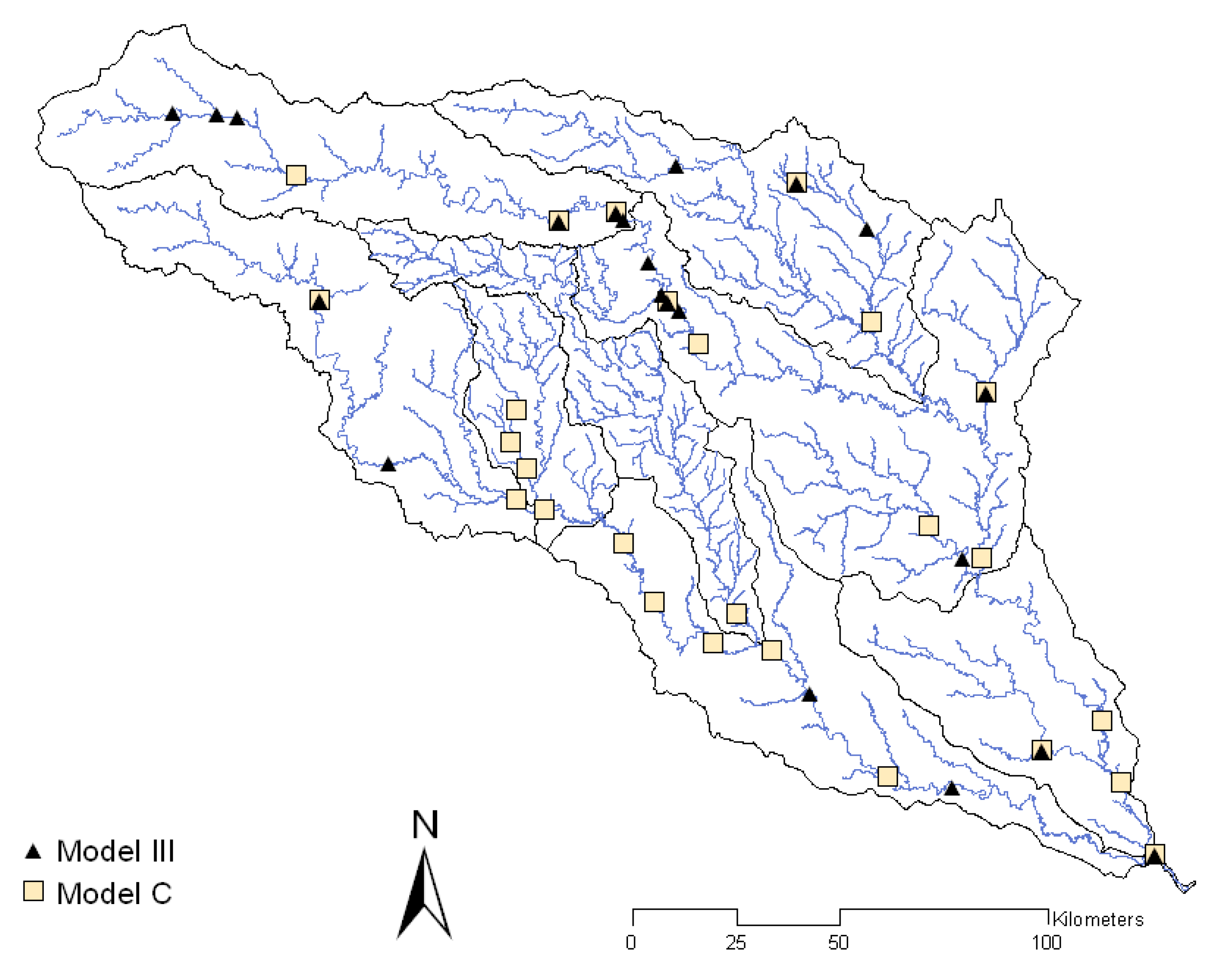
The previous study [13] applied FLUXMASTER to estimate the standard error to mean annual flux ratios for the monitoring stations; sets of monitoring stations were chosen based on those ratios. The optimal model from that study (Model III) was used for comparison with those chosen by the GA. Model III included only monitoring stations with a standard error to mean annual flux ratio that was less than or equal to 0.6, resulting in 21 monitoring stations.
3. Results and Discussion
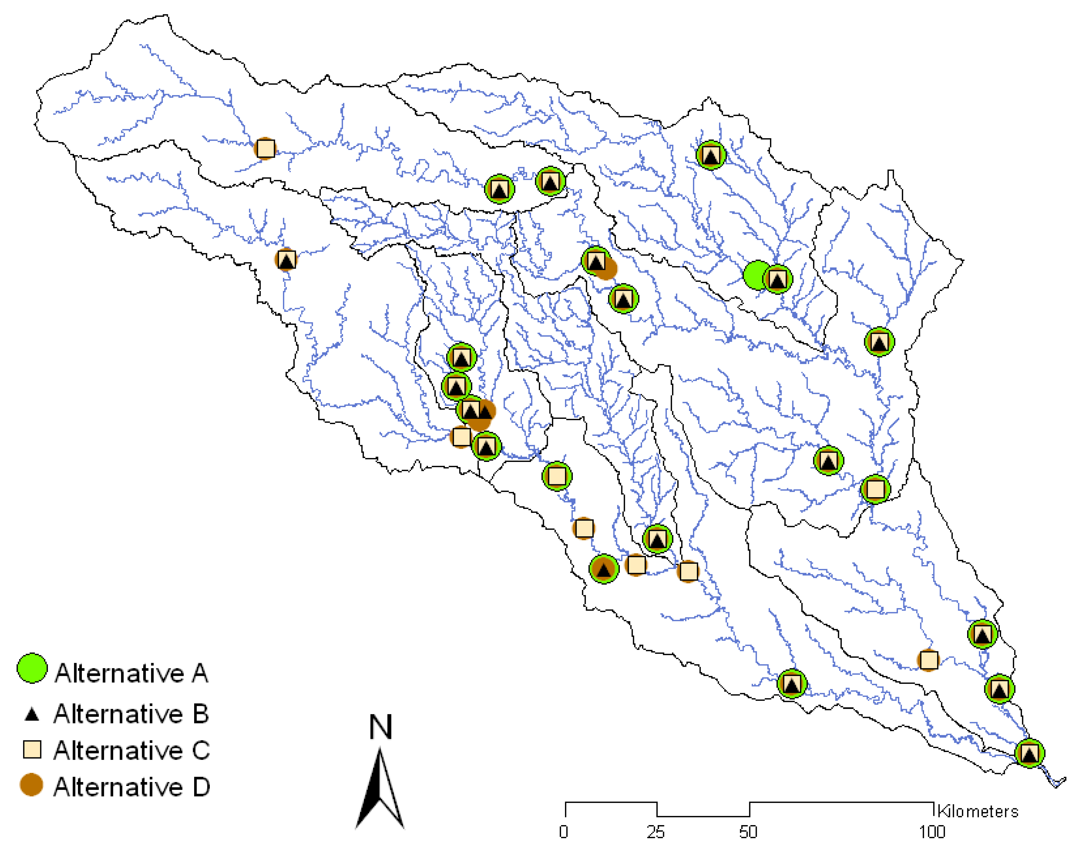
As alternatives to the selected model from the previous study [13], four optimized sets of monitoring stations were identified by applying the modified MOEA. The corresponding objective values and statistical indices of the alternative models (A–D) were compared to Model III (Table 1). The number of selected monitoring stations in the optimized sets varied from 20 to 30. The optimized sets contained fewer monitoring stations than those available in the basin. A reduction of monitoring stations could result in a decrease of monitoring costs. Additionally, the maintenance of fewer monitoring stations could enable longer durations of recorded monitoring for the same cost as maintaining more stations with shorter durations. Longer monitoring records may also allow better E. coli flux predictions using SPARROW.
The majority of the selected monitoring stations were common among the alternatives (Figure 3). Model B had the lowest number of monitoring stations (Objective 1), lowest average flux (Objective 2), and the least uncertainty in the predicted flux (Objective 3) among all alternatives (Table 1). If cost reduction were the priority, Model B would be the best option. However, this model has poor agreement with observed values. Because Model D had the highest number of monitoring stations, highest average flux, and the greatest uncertainty in the predicted flux (Table 1), that set of monitoring stations would not be ideal.
The average of log mean annual flux (Objective 2) for Model III was lower than the alternatives identified using the modified MOEA. This implies that Model III did not include many monitoring stations with high mean annual flux values. However, the statistical indices of the alternatives did not indicate good agreement with observed values. For instance, the AIC values were large for the alternatives, suggesting that the complex processes affecting E. coli flux were not accurately represented. Only Model C and Model III had NSE values that showed good agreement between the predicted and observed values.
Because SPARROW is a regression model, the results are affected by exceptionally high or low values of the mean annual flux. The PBIAS was lowest for Model C (3.20%), indicating only minimal overestimation of the mean annual flux. However, the inclusion of extremely high values of flux may have introduced non-negligible bias in the other models. Therefore, the inclusion of outliers may result in an inaccurate understanding of the watershed processes and can ignore actual sources of contaminants in the model results.
The SPARROW model was applied to each of the alternative sets of monitoring stations. The coefficients for the sources, land-water delivery, and stream/reservoir attenuation factors were determined, and then analyzed for significance (Table 2). Based on the selected monitoring locations and differences in the E. coli flux, some non-point sources were excluded during the calibration of SPARROW for specific models; for example, forest land use did not contribute E. coli in Models A, B, or C. Urban land was identified as an E. coli source for all of the models. Pasture land was considered an E. coli source for all alternative models, but not for Model III. Forest land use was considered a significant source (p < 0.25) of E. coli for Model III, but not for alternative C. Model C land-water delivery factor of temperature differed considerably from the other models (Table 2). Reach slope was only included in Model C, but not in the other models. Rainfall was only included in Model B, with a negative coefficient; this suggested that a dilution effect may lower the E. coli flux estimation.
Model C includes point sources as a significant contributor of E. coli. However, Model D did not include any significant point sources of E. coli. For Models A, B and III, the selected monitoring stations were not located downstream from point sources with high permitted flows and thus excluded from the models. Model C had the lowest RMSE and the most degrees of freedom (9). In contrast Model A had the least degrees of freedom (5), suggesting it was the least complex model. Model C can be considered a good alternative based on the objective values and statistical indices (Table 1 and Table 2).
Because Model C was suggested as the more accurate model among those identified by the application of the GA, it was chosen for further comparison with Model III (Figure 4). From the previous study, Model III had the lowest sum of square error and RMSE and also the highest R2. Unlike Model III, Model C selected a majority of monitoring stations in the highly contaminated Edwards Aquifer contributing zone and the City of San Antonio; these are critical areas that require rigorous monitoring.
For Model III, forest and urban lands were significant sources of E. coli, whereas, for Model C, only point sources were significant sources. Based on the statistical indices, Model III appears to be a better model than Model C based on lower AIC and higher NSE values. However, if considering regression error statistics (RMSE and R2), Model C is a better representation than Model III. Based on percent bias, neither Model III nor Model C showed a systematic tendency to under or overestimate the mean annual E. coli flux (Table 1).
In the earlier application of SPARROW by Smith, monitoring stations were selected based on the standard error [14]. The previous study by Puri used only the standard error to flux ratio to determine monitoring station sets, which resulted in an insufficient number of monitoring stations in the San Antonio River basin [13]. However, the GA generated alternative sets that adequately represented the San Antonio River basin. This shows agreement with the previous application of SPARROW which concluded that the San Antonio River basin required more rigorous monitoring [13]. The application of the GA ensured the inclusion of the monitoring stations with large values of E. coli flux for the application of SPARROW.
4. Conclusions
In this study, a GA was applied to select monitoring stations based on specified objectives and constraints. The SPARROW model was then applied to the optimum solution sets. From the previous study, stations selected solely based on the standard error to mean annual flux ratio (Model III) did not adequately represent highly contaminated areas. However, the best monitoring set (Model C) from the GA-optimized solutions included adequate coverage for those areas that require rigorous monitoring, such as the Edwards Aquifer contributing zone and the City of San Antonio. The locations of monitoring stations play a crucial role in accurately representing the water quality in a basin. A GA algorithm was successfully used to optimize the selection of monitoring stations in a water quality network.
Acknowledgments
We acknowledge the technical critique provided by Meghna Babbar-Sebens and Emily Zeckman when they were associated with Texas A & M University.
Author Contributions
Deepti Puri and Raghupathy Karthikeyan conceptualized the model. Deepti Puri conducted the analyses. Deepti Puri, Kyna Borel, Cherish Vance, and Raghupathy Karthikeyan wrote and edited the manuscript.
Conflicts of Interest
The authors declare no conflict of interest.
References
- Park, S.; Choi, J.H.; Wang, S.; Park, S.S. Design of a water quality monitoring network in a large river system using the genetic algorithm. Ecol. Model. 2006, 199, 289–297. [Google Scholar] [CrossRef]
- USEPA Consolidated Assessment and Listing Methodology: Toward a Compendium of Best Practices; EPA: Zurich, Switzerland, 2002.
- Holland, J.H. Genetic algorithms. Sci. Am. 1992, 267, 66–73. [Google Scholar] [CrossRef]
- Savic, D.; Khu, S. Evolutionary computing in hydrological sciences. In Encyclopedia of Hydrological Sciences; John Wiley & Sons, Inc.: Hoboken, NJ, USA, 2005. [Google Scholar]
- Srivastava, P.; Hamlett, J.M.; Robillard, P.D.; Day, R.L. Watershed optimization of best management practices using AnnAGNPS and a genetic algorithm. Water Resour. Res. 2002, 38. [Google Scholar] [CrossRef]
- Yandamuri, S.R.; Srinivasan, K.; Murty Bhallamudi, S. Multiobjective optimal waste load allocation models for rivers using nondominated sorting genetic algorithm-II. J. Water Resour. Plan. Manag. 2006, 132, 133–143. [Google Scholar] [CrossRef]
- Icaga, Y. Genetic algorithm usage in water quality monitoring networks optimization in Gediz (Turkey) river basin. Environ. Monit. Assess. 2005, 108, 261–277. [Google Scholar] [CrossRef] [PubMed]
- Reed, P.; Minsker, B.; Goldberg, D.E. Designing a competent simple genetic algorithm for search and optimization. Water Resour. Res. 2000, 36, 3757–3761. [Google Scholar] [CrossRef]
- Reed, P.; Minsker, B.S.; Goldberg, D.E. A multiobjective approach to cost effective long-term groundwater monitoring using an elitist nondominated sorted genetic algorithm with historical data. J. Hydroinf. 2001, 3, 71–89. [Google Scholar]
- Riebschleager, K.J.; Karthikeyan, R.; Srinivasan, R.; McKee, K. Estimating Potential E. coli Sources in a Watershed Using Spatially Explicit Modeling Techniques. J. Am. Water Resour. Assoc. 2012, 48, 745–761. [Google Scholar]
- Shirmohammadi, A.; Chaubey, I.; Harmel, R.D.; Bosch, D.D.; Muoz-Carpena, R.; Dharmasri, C.; Sexton, A.; Arabi, M.; Wolfe, M.L.; Frankenberger, J. Uncertainty in TMDL models. Trans. ASABE 2006, 49, 1033–1049. [Google Scholar] [CrossRef]
- McMahon, G.; Alexander, R.B.; Qian, S. Support of total maximum daily load programs using spatially referenced regression models. J. Water Resour. Plan. Manag. 2003, 129, 315–329. [Google Scholar] [CrossRef]
- Puri, D.; Karthikeyan, R.; Babbar-Sebens, M. Predicting the fate and transport of E. coli in two Texas river basins using a spatially referenced regression model. JAWRA J. Am. Water Resour. Assoc. 2009, 45, 928–944. [Google Scholar] [CrossRef]
- Smith, R.A.; Schwarz, G.E.; Alexander, R.B. Regional interpretation of water-quality monitoring data. Water Resour. Res. 1997, 33, 2781–2798. [Google Scholar] [CrossRef]
- NHDPlus Texas Data (Vector Processing Unit 12). Available online: https://www.epa.gov/waterdata/nhdplus-texas-data-vector-processing-unit-12 (accessed on 12 September 2017).
- Clean Rivers Program. Available online: http://gbra.org/crp/default.aspx (accessed on 12 September 2017).
- Clean Rivers Program. Available online: https://www.sara-tx.org/environmental-science/clean-rivers-program/ (accessed on 12 September 2017).
- USGS Surface-Water Data for USA. Available online: https://waterdata.usgs.gov/nwis/sw (accessed on 8 July 2007).
- USEPA, Envirofacts. Available online: https://www3.epa.gov/enviro/ (accessed on 12 September 2017).
- Center for Environmental Informatics. Available online: http://www.cei.psu.edu/ (accessed on 12 September 2017).
- The SPARROW Surface Water-Quality Model: Theory, Application and User Documentation. Available online: https://pubs.usgs.gov/tm/2006/tm6b3/ (accessed on 12 September 2017).
- Eiben, A.E.; Smith, J.E. Natural Computing Series. In Introduction to Evolutionary Computing; Springer: New York, NY, USA, 2003; Volume 53, pp. 36–51. [Google Scholar]
- Grefenstette, J.J. Optimization of control parameters for genetic algorithms. IEEE Trans. Syst. Man Cybern. 1986, 16, 122–128. [Google Scholar] [CrossRef]
- Konak, A.; Coit, D.W.; Smith, A.E. Multi-objective optimization using genetic algorithms: A tutorial. Reliab. Eng. Syst. Saf. 2006, 91, 992–1007. [Google Scholar] [CrossRef]
- Zitzler, E.; Deb, K.; Thiele, L. Comparison of multiobjective evolutionary algorithms: Empirical results. Evol. Comput. 2000, 8, 173–195. [Google Scholar] [CrossRef] [PubMed]
- Sarker, R.; Liang, K.; Newton, C. A new multiobjective evolutionary algorithm. Eur. J. Oper. Res. 2002, 140, 12–23. [Google Scholar] [CrossRef]
- Schwarz, G.E.; Hoos, A.B.; Alexander, R.B.; Smith, R.A. The SPARROW surface water-quality model: Theory, application and user documentation. In US Geological Survey Techniques and Methods Report; USGS: Reston, VA, USA, 2006. [Google Scholar]
- Moriasi, D.N.; Arnold, J.G.; Van Liew, M.W.; Bingner, R.L.; Harmel, R.D.; Veith, T.L. Model evaluation guidelines for systematic quantification of accuracy in watershed simulations. Trans. ASABE 2007, 50, 885–900. [Google Scholar] [CrossRef]
Figure 1.
Monitoring stations and major streams in the Guadalupe and San Antonio River Basins.
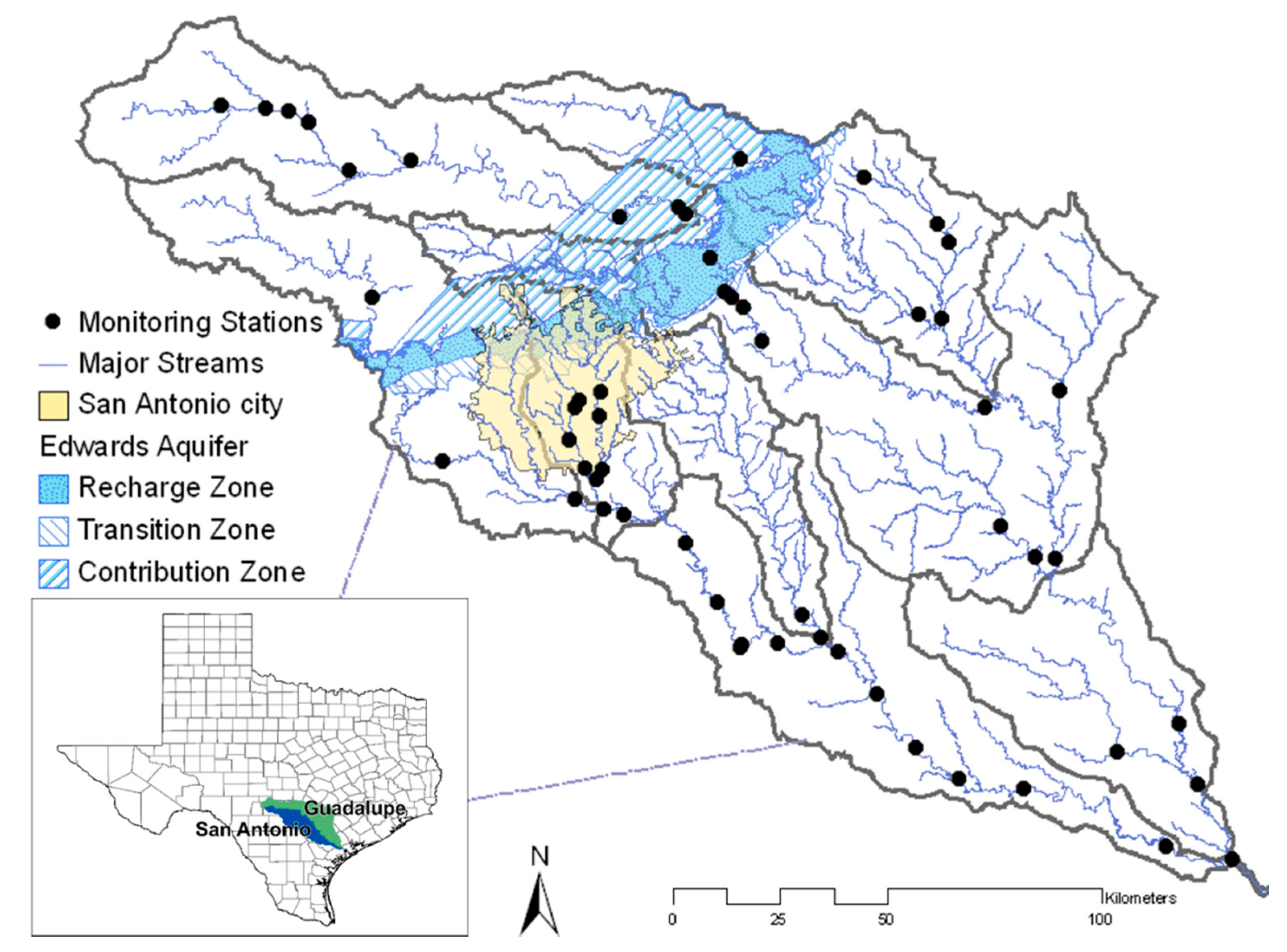
Figure 2.
Modified multi-objective evolutionary algorithm (MOEA).

Figure 3.
Four alternative sets of monitoring stations obtained after the application of the modified MOEA.
Figure 3.
Four alternative sets of monitoring stations obtained after the application of the modified MOEA.

Figure 4.
Monitoring stations selected in Model C and Model III.

Table 1.
Objectives and statistical indices for the alternative models (A–D) and Model III.
| Objectives and Statistical Indices | A | B | C | D | III |
|---|---|---|---|---|---|
| Number of selected monitoring stations | 21 | 20 | 26 | 30 | 21 |
| Average of log mean annual flux | 18.13 | 17.13 | 21.37 | 25.82 | 5.50 |
| Sum of standard error to mean annual flux ratio | 16.14 | 14.89 | 19.01 | 22.61 | 7.7 |
| Akaike Information Criteria (AIC) | 874.20 | 840.40 | 824.41 | 1249.20 | 101.50 |
| Nash– Sutcliffe Efficiency (NSE) | −0.05 | 0.00 | 0.57 | −0.03 | 0.88 |
| Percent Bias (PBIAS) | 52.70 | 67.00 | 3.20 | 79.13 | 28.00 |
Table 2.
Model coefficients and p-values (in) for the source, land–water delivery, and stream/reservoir attenuation factors.
Table 2.
Model coefficients and p-values (in) for the source, land–water delivery, and stream/reservoir attenuation factors.
| Model | A | B | C | D | III |
|---|---|---|---|---|---|
| Selected Monitoring Stations | 21 | 20 | 26 | 30 | 21 |
| Sources | |||||
| Point sources discharge (m3 year−1) | -- | -- | 0.49 (0.22) | 0.48 (0.42) | -- |
| Pasture land (m2) | 13.98 (0.13) | 7.29 (0.19) | 0.19 (0.32) | 36.74 (0.13) | -- |
| Forest land (m2) | -- | -- | 1.41 × 10⁻⁵ (0.50) | -- | 0.73 (0.06) |
| Urban land (m2) | 3.52 (0.22) | 3.23 (0.25) | 4.2 × 10⁻³ (0.32) | 9.48 (0.26) | 0.94 (0.12) |
| Delivery Factors | |||||
| Rainfall (m) | -- | −5.03 (0.20) | -- | -- | 4.59 (0.24) |
| Temperature (°C) | 1.75 (<0.01) | 1.74 (<0.01) | −0.26 (0.23) | 1.09 (0.02) | 2.41 (<0.01) |
| Drainage density (km−1) | 2.19 (0.01) | 1.60 (0.13) | 3.03 (<0.01) | 2.71 (<0.01) | -- |
| Permeability (cm h−1) | -- | 0.14 (0.30) | -- | −0.01 (0.89) | −0.08 (0.36) |
| Reach slope (%) | -- | -- | −12.20 (<0.01) | -- | -- |
| Reservoir/Stream Decay Factors | |||||
| Areal hydraulic load (m·year−1) | -- | -- | 30.18 (0.39) | 218.85 (0.47) | -- |
| Medium-sized stream (0.02 < flow ≤ 0.13 m3 s−1) | 13.38 (0.02) | 14.99 (0.02) | 13.52 (1.1 × 10⁻³) | 17.12 (0.02) | 13.38 (0.02) |
| Sum of Square Error | 30.45 | 26.03 | 14.67 | 49.87 | 18.27 |
| Root Mean Square Error (RMSE) | 1.34 | 1.41 | 0.93 | 1.50 | 1.14 |
| Coefficient of Determination (R2) | 0.62 | 0.72 | 0.86 | 0.67 | 0.85 |
| Degrees of Freedom | 5 | 7 | 9 | 8 | 6 |
Note: -- Source or factor excluded during the calibration of SPARROW because of the locations of the monitoring stations.
© 2017 by the authors. Licensee MDPI, Basel, Switzerland. This article is an open access article distributed under the terms and conditions of the Creative Commons Attribution (CC BY) license (http://creativecommons.org/licenses/by/4.0/).
Share and Cite
MDPI and ACS Style
Puri, D.; Borel, K.; Vance, C.; Karthikeyan, R. Optimization of a Water Quality Monitoring Network Using a Spatially Referenced Water Quality Model and a Genetic Algorithm. Water 2017, 9, 704. https://doi.org/10.3390/w9090704
AMA Style
Puri D, Borel K, Vance C, Karthikeyan R. Optimization of a Water Quality Monitoring Network Using a Spatially Referenced Water Quality Model and a Genetic Algorithm. Water. 2017; 9(9):704. https://doi.org/10.3390/w9090704
Chicago/Turabian StylePuri, Deepti, Kyna Borel, Cherish Vance, and Raghupathy Karthikeyan. 2017. "Optimization of a Water Quality Monitoring Network Using a Spatially Referenced Water Quality Model and a Genetic Algorithm" Water 9, no. 9: 704. https://doi.org/10.3390/w9090704
Note that from the first issue of 2016, this journal uses article numbers instead of page numbers. See further details here.