Threshold of Slope Instability Induced by Rainfall and Lateral Flow


1
IHE Delft Institute for Water Education (UNESCO-IHE), 2611 AX Delft, The Netherlands
2
Department of Civil and Water Resources Engineering, National Chiayi University, Chiayi 60004, Taiwan
3
Department of Civil Engineering, National Chiao Tung University, Hsinchu 30010, Taiwan
*
Author to whom correspondence should be addressed.
Water 2017, 9(9), 722; https://doi.org/10.3390/w9090722
Submission received: 25 July 2017
/
Revised: 14 September 2017
/
Accepted: 18 September 2017
/
Published: 20 September 2017
Abstract
:In this study, a two-dimensional numerical landslide model was developed to investigate the effects of the amount of rainfall and lateral flow on induced slope failures. The Richard’s equation was used to evaluate pore water pressure distribution in response to moisture content variations induced by rainfall and infiltration in soil mass. The slope stability was then assessed using the limit equilibrium method of slices, and the moment equilibrium was considered. Several hypothetical cases involving various rainfall amounts and durations were simulated using the proposed model to investigate the possible tendency toward slope instability caused by rainfall time-series processes. After the rainfall conditions were analyzed, rainfall patterns were categorized as uniform, intermediate, advanced, and delayed types. Furthermore, the lateral flows running through the upstream and downstream boundaries of a slope were analyzed to investigate the lateral effects on the hillslope. The results indicated that the lateral flow may increase or reduce the groundwater table and, thus, accelerate or reduce the occurrence of slope failure. In addition, several rainfall threshold curves that accounted for the rainfall amounts, durations, and patterns were developed and appeared more realistic and to approximate real conditions more accurately than those created using one-dimensional landslide modeling do.
1. Introduction
Rainfall-induced landslides have posed a serious threat to human lives and property at many locations worldwide. The rainfall threshold concept is commonly applied to landslide forecasting and early warning systems to prevent the disastrous consequences of landslides that occur during unusual precipitation events. Thresholds of slope instability can generally be obtained by using physical or empirical approaches. The empirical threshold for landslide occurrence can be simply derived from either the critical cumulative rainfall amount [1] or the rainfall intensity [2]. Caine [3] studied the effects of rainfall intensity and duration. Several studies [4,5,6] have investigated the climatic effect on slope stability by normalizing rainfall intensity to the mean annual rainfall amount. Govi et al. [7] developed another frequently used rainfall threshold method that involves correlating the amount of accumulated rainfall until a landslide is initiated with the maximum rainfall intensity. In addition, Glade [8] considered the influence of antecedent rainfall on the rainfall threshold in landslide occurrences.
As mentioned previously, the empirical rainfall threshold for landslide occurrences has been comprehensively studied to examine all of the possible effects of hydrological factors, including the rainfall amount, the rainfall duration, the mean rainfall intensity, the maximum hourly rainfall intensity, and the antecedent rainfall. However, physical processes, such as the hydrodynamic and geotechnical mechanisms, are not considered in empirical approaches to analyzing hillside failure, and empirical approaches can be influenced strongly by site-specific conditions, especially the physical and mechanical properties of hillslope materials. Therefore, several studies [9,10,11,12] have proposed physical-process-based numerical approaches. Many researchers, such as Tarantino and Bosco [13], Collins and Znidarcic [14], and Tsai et al. [15] have investigated shallow landslide models by using the Richards’ equation and have extended the Mohr–Coulomb failure criterion [16] to describe the shear strength of unsaturated soil. Furthermore, physical-process-based models that involve the hydrological modeling of nearly saturated soil [17,18,19] have commonly been used for assessing rainfall-triggered shallow landslides [20,21,22,23,24,25,26,27,28,29].
Tsai [11] applied the modified Iverson’s model [19] to investigate the influences of rainfall patterns on shallow landslides in saturated soils caused by increases in the groundwater table. Tsai and Wang [12] examined the effects of rainfall patterns on shallow landslides in unsaturated soils caused by the dissipation of matric suction. Based on the one-dimensional landslide model, Tsai [11] presented the rainfall threshold for representative rainfall patterns. However, one-dimensional modeling cannot be used to investigate the influence of boundary conditions with lateral inflow and outflow. Two-dimensional infiltration modeling has been combined with the limit equilibrium slope stability method [9,14,30] to assess landslides, and the lateral flow and boundary effects were considered.
In this study, to reliably evaluate landslides, a physical–process-based model was developed using the two-dimensional Richards’ equation and the limit equilibrium slope stability method to simulate local hillslope instability phenomena. The mathematical basis and computational procedure for the two-dimensional landslide model is introduced in the following sections. Using the established landslide model, this study investigated the effects of rainfall amount and patterns on landslides. The results revealed that rainfall threshold curves with various durations and amounts clarified the effects of lateral flows on slopes and illustrated the advantages of using two-dimensional landslide modeling instead of one-dimensional modeling.
2. Mathematical Basis
Infiltration flow is an essential triggering mechanism that must be addressed when studying slope failure after a period of heavy rainfall. In this study, both saturated and unsaturated infiltration flows were considered in evaluating pore water pressures by solving the two-dimensional Richards’ equation. The pore water pressures were then used to evaluate the factor of safety (FS) of a hillslope by applying the Bishop slope stability analysis method. This study only focuses on analyzing a particular site or a slope. The theory of infiltration equation and slope stability analysis are briefly described in this section.
2.1. Infiltration Equation
The governing Equation [31] for calculating the groundwater flow in response to rainfall infiltration on a hillslope can be obtained using the Richards’ equation with a local rectangular Cartesian coordinate system as follows:
where t is time; is the moisture content; is the pore water pressure head; and and are hydraulic conductivities in the x and z directions, respectively, in a function of soil properties.
A solution of Equation (1) was obtained using the appropriate initial and boundary conditions. Regarding an initial steady state with a water table of dZ in a vertical direction, the initial condition in terms of the pressure head are expressed as
where is the elevation. The boundary condition subjected to rainfall intensity at ground surface of hillslope can be expressed as:
where is the slope angle. When the ground surface is saturated, the pressure head of the ground surface is equal to zero; thus, the boundary condition can be expressed as
Solving Equations (1)–(4) requires a relationship among pressure, moisture content, and hydraulic conductivity. For isotropic soils with respect to hydraulic conductivity K = Kx = Kz, the function of the water retention curve proposed by van Genuchten [32] was employed in this study:
where S is the degree of saturation; is saturated hydraulic conductivity; denotes the saturated moisture content; represents the residual moisture content; and , N, and M are the fitting parameters ().
2.2. Slope Stability Analysis
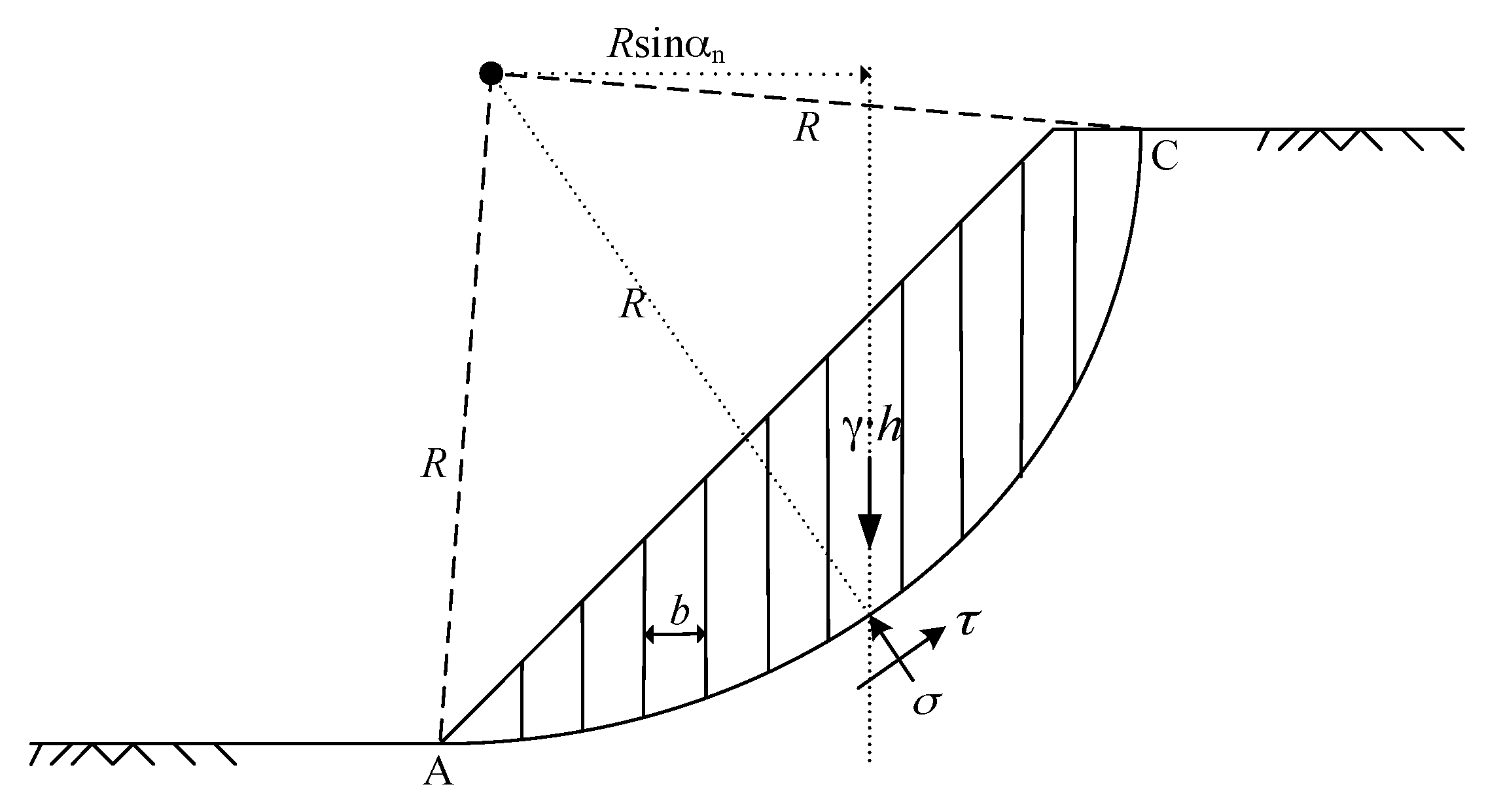
The stability of slopes is commonly analyzed using the limit equilibrium method of slices [33] and based on a consideration of the moment equilibrium of soil mass. The soil mass is subdivided into a number of vertical slices that exhibit a width bn above an assumed circular slip surface (Figure 1). The maximum shear stress of unsaturated soil acting at the lower boundary of a slice is related to the total normal stress according to the Mohr–Coulomb failure criterion [16] and is expressed as follows:
where c′ is the effective cohesion; and are, respectively, the angle of shearing resistance and friction angle with respect to the matric suction; and ua and uw denote the pore air pressure and pore water pressure, respectively. Evidently, when the soil is saturated, ua and uw become equal, and Equation (7) reverts to the classical shear strength of saturated soil as follows:
Equations (7) and (8) are used to evaluate the shear strength of soil in physical models based on hydrological modeling in nearly saturated soil [17,18,19].
The shear stress acting on the lower boundary of a slice is assumed to be . Hence,
The equilibrium of moments relative to the center of the slip circle can be expressed by equating the sum of the moments of the weight of each slice relative to the center of the circle to the sum of the moments of the shearing forces at the bottom of the slices. The depth-averaged unit weight in a slice can be expressed as
where Gs is the specific gravity of a soil solid, such that the weight of each slice is . Therefore, the equilibrium of the moments can be expressed as
where is the width of each slice, is the height of each slice. If all slices exhibit the same width, then the FS can be derived from Equations (9) and (11) as follows:
In Bishop’s method [33], the force transmitted between adjacent slices is assumed to be strictly horizontal. According to the vertical equilibrium of a slice,
When using Equation (9) to calculate the shear stress, the following expression is obtained:
This expression can be substituted into Equation (12), yielding the following FS:
When using Equation (12) together with the shear strength of unsaturated soil given by Equation (7), and assuming that the pore air pressure is atmospheric, the FS in Equation (15) can be expressed as
where represents the unit weight of water. In Equation (16), when the groundwater pressure head becomes negative, the soil is unsaturated, and is equal to , which can be obtained from Equation (1), whereas is zero. Conversely, when the groundwater pressure head becomes positive, is identical to , is zero, and the soil is saturated. Equation (16) reveals that slope failure occurs not only in saturated soil because of an increase in the positive groundwater pressure head but also in unsaturated soil because of a decrease in the negative groundwater pressure head, indicating that a dissipation of matric suction has occurred.
The physical-based method of landslide simulation has high accuracy in the condition of adopting the field-measured data and laboratory test data. However, it ignores the other factors such as vegetation or drainage.
3. Computational Procedure
To solve the Richards’ equation in Equation (1), the implicit finite-difference scheme [34] was applied. When using a backward finite-difference approximation of the time derivative and assuming two-dimensional propagation occurs along the x-z direction, Equation (1) becomes
where is the approximated value of at time step n and iteration m; and and ; is expanded in a Taylor series as follows:
where represents all higher-order terms. When substituting Equation (18) into Equation (17) and neglecting higher-order terms, this equation yields
When using central-difference approximation to calculate the partial derivative of with respect to the x and z directions, Equation (19) can be expanded into the following form:
where i and j represent the discrete points; and and represent the nodal space in the x and z directions, respectively.
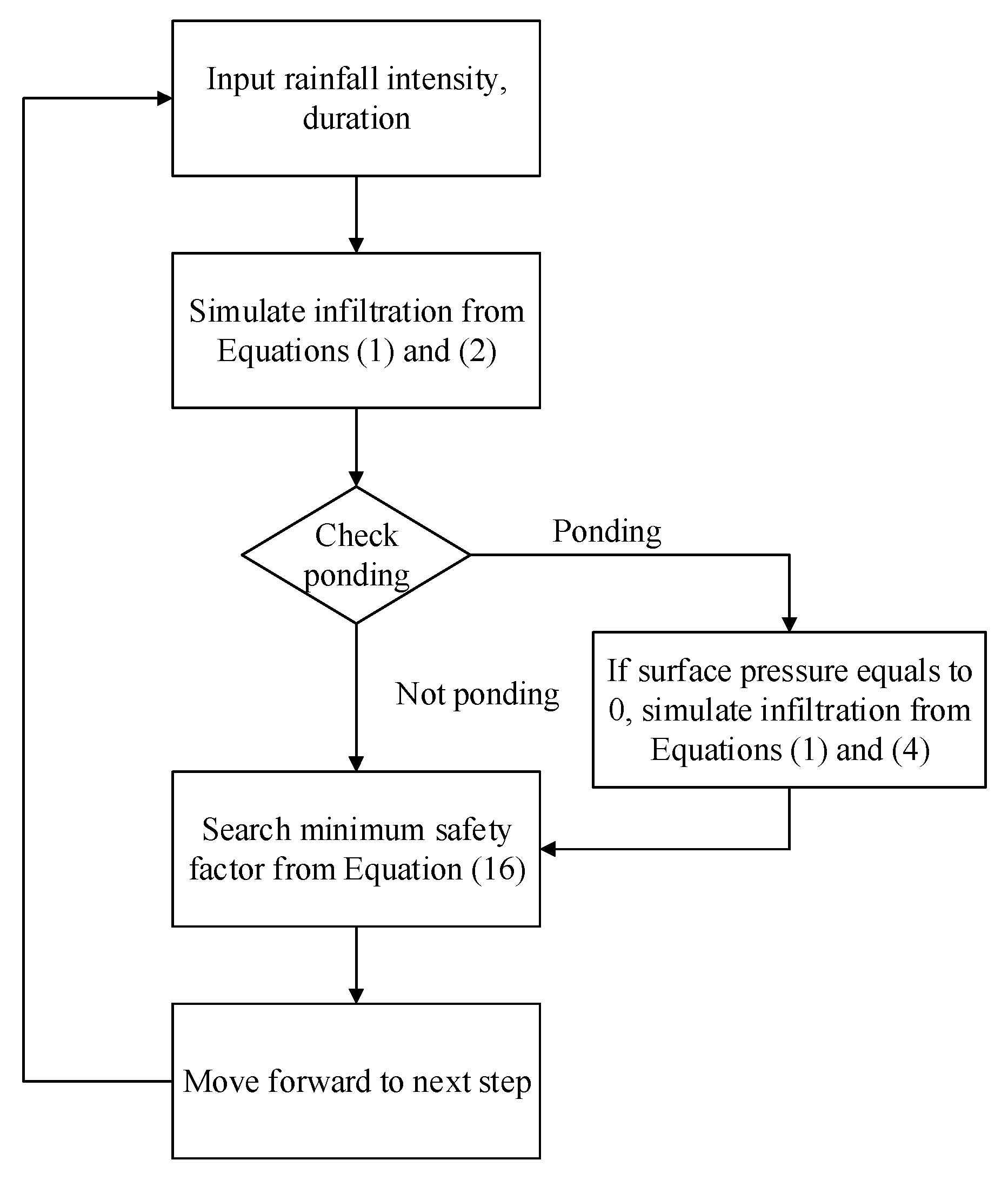
Equations (17)–(20) require an iterative procedure (Figure 2) to be solved numerically because of their nonlinearity. The groundwater pressure head at the ground surface of a hillslope is first obtained by assuming that the infiltration rate equals the rainfall intensity shown in Equation (3). If the pressure head on the slope surface is less than or equal to zero, then ponding does not occur and the calculated results are acceptable. The computation moves forward to the next time step. If the calculated pressure head on the slope surface is greater than zero, then ponding occurs, when the water depth of overland flow is neglected, and the zero pressure head can be used as a boundary condition to recalculate once in the same time step. The computed pore water pressures in the slopes are substituted into Equation (16) to evaluate the FS of a circular slip surface. The same procedure is performed to determine the minimum FS at various slip surfaces.
4. Effect of Rainfall Amount
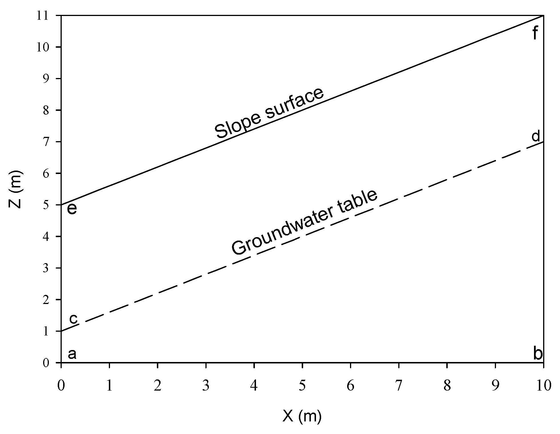
To clearly observe the rainfall and lateral flow effects, a specific geometrical and physical case were adopted. Figure 3 shows that the case slope geometry exhibited an angle of 31° and height of 6 m. This slope was like a slope from the hilltop to the mid or the bottom. Thus, this case can ignore surface flow or infiltration from the upper side of the slope. The boundary conditions are listed as follows: ab represented impervious boundaries (rock masses); ae and bd represented the Dirichlet boundaries with a prescribed total water head; df represented no flux boundary; and ef was the ground surface subjected to rainfalls. The initial groundwater table was 4 m below the ground surface of the hillslope. The soil parameters in the case study are listed as follows: = 0.47; = 0.17; = 0.031 m/h; N = 2; M = 0.5; = 0.01; c′ = 500 N/m2; = 26°; = 13°; and = 2.65. The soil was classified as sandy loam [32].
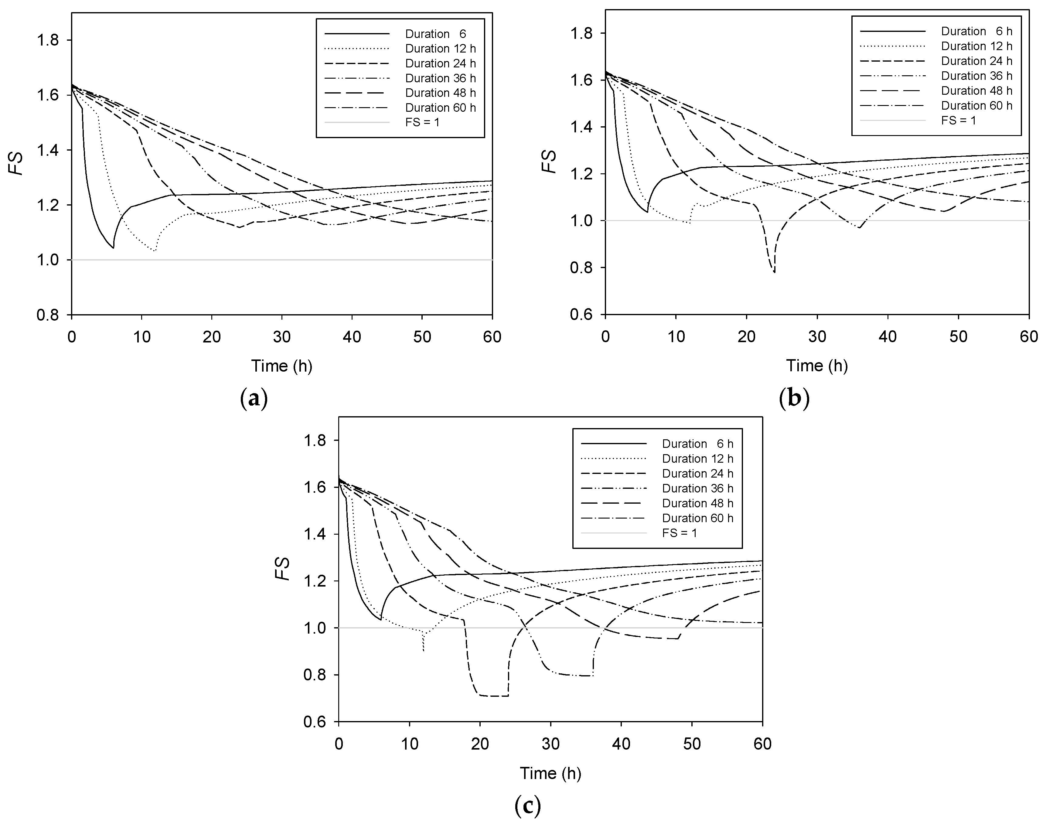
Figure 4 shows the simulated results of the FS with respect to time for various rainfall durations in which the uniform rainfall amounts were 300, 400, and 500 mm, indicating that the FS decreased over time during rainfall. After the rainfall, the FS increased over time and the minimum FS appeared at the end of the rainfall period. For the 300-mm rainfall events (Figure 4a), all the FS were greater than 1.0 that the slope were stable during the various duration. Figure 4b shows that the 400-mm rainfall events that occurred over durations of 12-h, 24-h, and 36-h triggered slope failure, during which the FS below 1.0 for 10.5 h, 22 h, and 34 h, respectively. Conversely, the 400-mm rainfall events that occurred during the 6-h, 48-h, and 60-h durations did not trigger slope failures. Furthermore, the decreasing rate of FS was faster in a shorter duration (higher intensity) when the amount of rainfall was the same. The results indicated that a higher rainfall intensity was more likely to trigger a slope failure when the rainfall duration was the same. However, when the amount of rainfall was the same, no consistent trend was observed. That is, there was no obvious positive or negative correlation between the length of duration and FS.
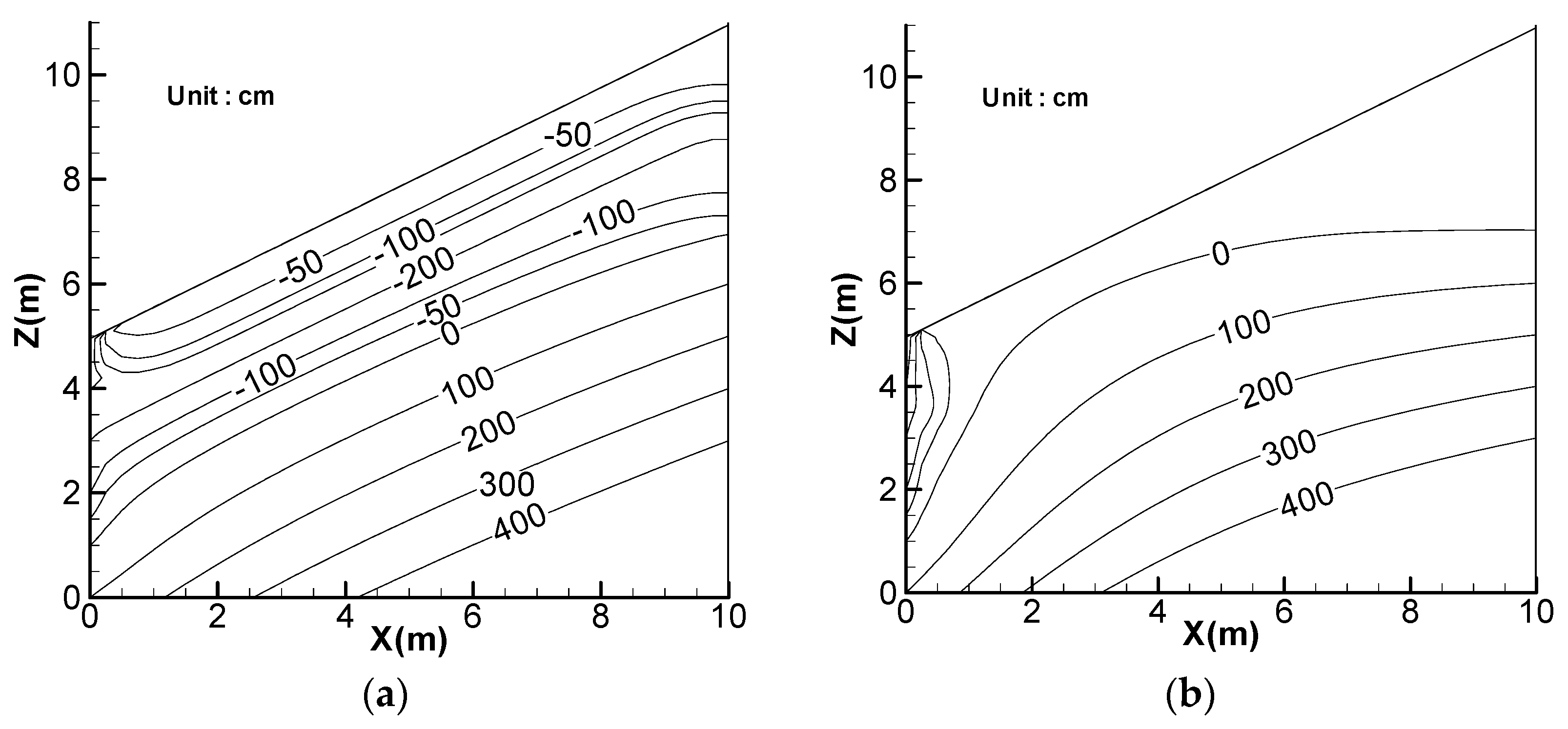
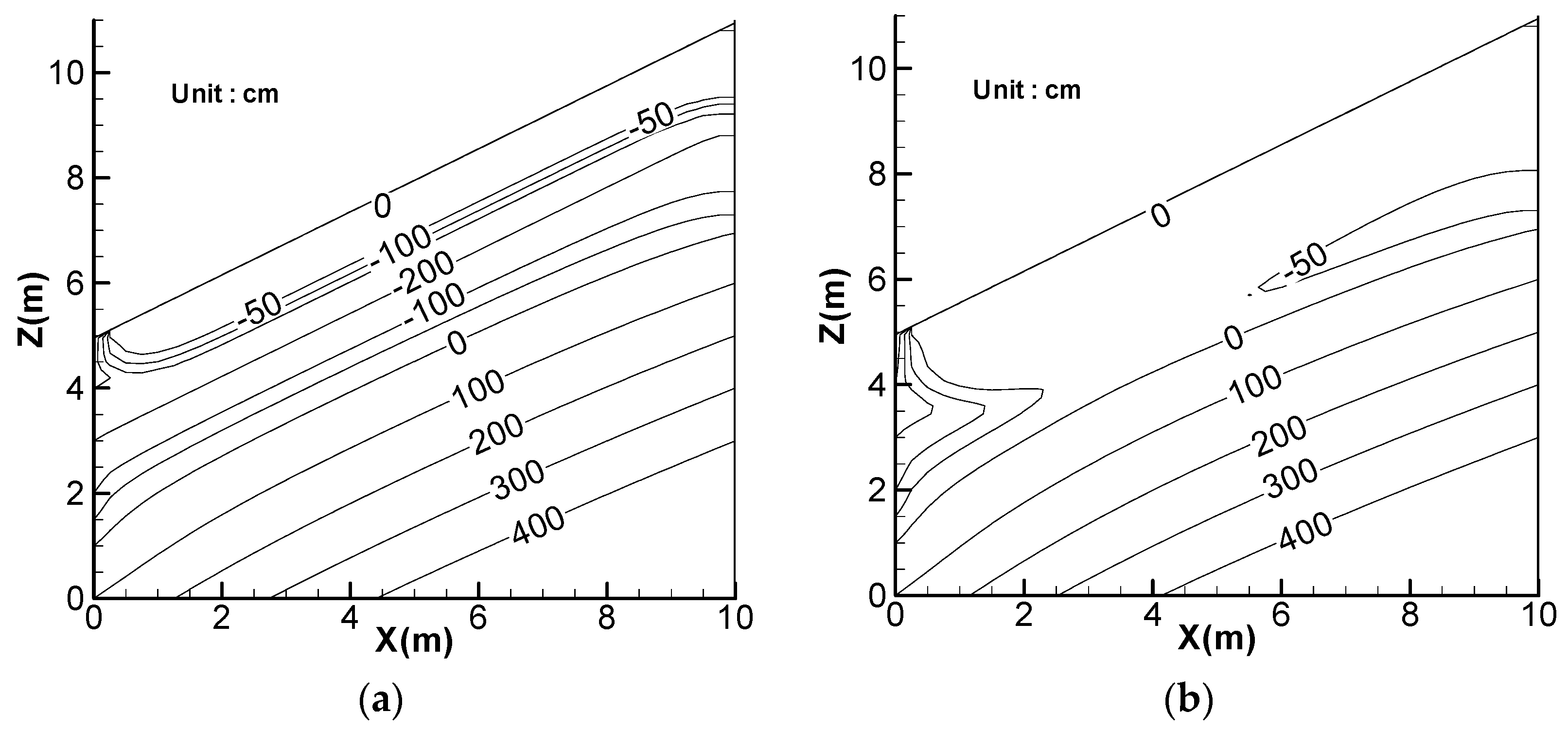
Figure 5 and Figure 6 show the simulated groundwater pressure heads relative to time for a 400-mm, 24-h rainfall event and a 500-mm, 36-h rainfall event. During the rainfall period, the wetting front propagated downward, as shown in Figure 5a,b, or Figure 6a,b. The matric suction decreased and the groundwater pressure heads increased relative to time. When no more water flowed into the slope, the pore water pressure remained similar over time, as shown in Figure 6c,d. This is the reason that in Figure 4c the values of FS versus time were approximated to a constant. After rainfall, the groundwater pressure heads decreased and the matric suction increased relative to time, as shown in Figure 6e.
5. Effect of Lateral Flow
In previous section, there was no obvious positive or negative correlation between the length of duration and FS. Thus, this section analyzed the correlation between the FS and rainfall infiltration or groundwater outflowed from the slope boundary. Figure 7a shows the accumulated rainfall infiltration during a 400-mm uniform rainfall event on the slope surface (boundary ef in Figure 3), indicating that, when the rainfall duration was longer than 24 h, all the water infiltrated into the slope, and the amount of infiltration during the 6-h duration was smaller than the 12-h duration. It indicated that a higher rainfall intensity is more likely to cause ponding that substantially influences the rainfall infiltration rate; thus, slope failure was less likely to occur in cases (Figure 4b) which the rainfall intensity was higher and the rainfall amount remained the same. As the ponding effect occurred, the true added water mass (inflow from boundaries bd and ef; outflow of boundary ae, in Figure 3) during longer rainfall durations was greater than that during the 6-h duration at the end of the rainfall period, as shown in Figure 7b. At the end of the rainfall period, the water mass added during the 24-h duration was greater than that added during the 48-h duration, indicating that groundwater outflows from the slope boundary were greater during the long rainfall time period and, therefore, a slope failure was not triggered (Figure 4b).
Figure 8 and Figure 9 show the pressure head contours for the 400-mm rainfall events during 6-h and 12-h durations, in which some of the rainfall ran off the slope surface because of the ponding effect. The water wetting front did not reach the groundwater table during a short rainfall period. The matric suction was unlikely to decrease in instances of increased rainfall intensity when the rainfall amount was the same. During the long rainfall period, the groundwater table increased because of an increase in positive pore water pressure (Figure 10 and Figure 11). The pressure head contours of the 400-mm rainfall events during the 36-h and 48-h durations indicated that the increased groundwater table decreased in cases in which the durations are long as a result of the lateral flow effect. Therefore, the lateral flow should be introduced to study the relationship between the rainfall duration and the FS. As the lateral flow affected the different results of slope failure, the anisotropy can also strongly influence the results.
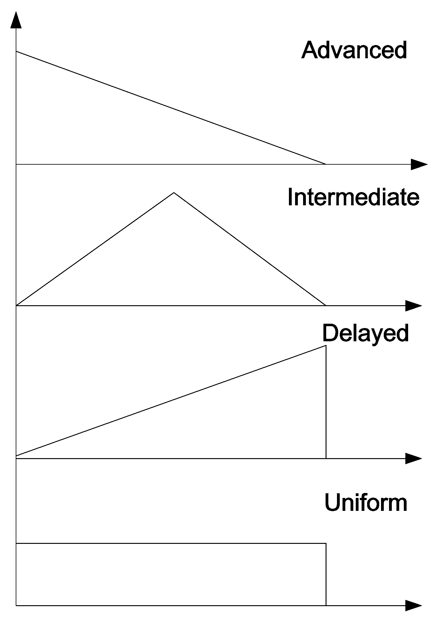
6. Effect of Rainfall Pattern
The various rainfall patterns in Figure 12 and hillslope conditions identical to those described in the previous section were considered in plotting the FS with respect to time for the 400-mm rainfall event during various rainfall durations and rainfall patterns (Figure 13). In each rainfall pattern, it is clear that the decreasing rate of FS was faster in a higher intensity when the amount of rainfall was the same, but the FS varied according to the rainfall pattern. Regarding the rainfall duration of 24 h, the intermediate rainfall pattern (Figure 13b) induced slope failures at 20 h and the delayed rainfall pattern (Figure 13c) induced slope failures at 21.5 h. The slope was stable when the advanced rainfall pattern (Figure 13b) was applied. In addition, the slope was stable during the rainfall event 48 h in duration when the advanced and intermediate rainfall patterns were applied. The delayed rainfall pattern induced slope failures at 44 h. Slope failure may or may not have occurred during various durations. As mentioned in Section 4 and Section 5, the rainfall duration causes significant effect on slope failure, and groundwater outflows from the sloped boundary may also affect slope stability; moreover, the results in this section revealed that the rainfall patterns play a role that also affects slope stability.
7. Discussion of Landslide Threshold
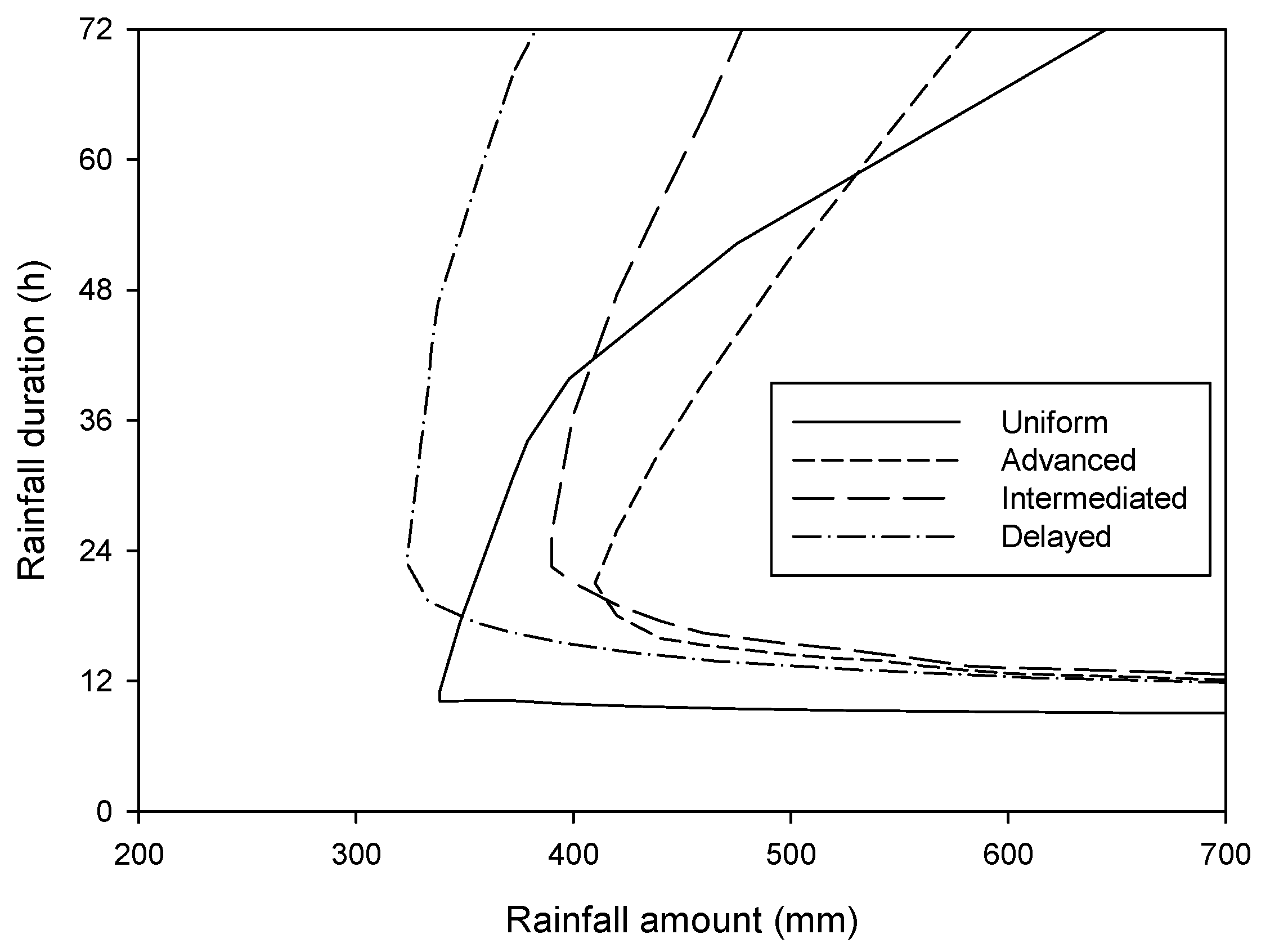
According to the results in Section 4, Section 5 and Section 6, the rainfall amount, the length of rainfall duration and the rainfall patterns may jointly affect the FS. Thus, in this section, we considered all these factors above and developed several threshold curves of slope instability induced by rainfall and lateral flow. The rainfall threshold curves were developed (Figure 14) based on the four representative rainfall patterns with various durations and amounts of rainfall. Figure 14 shows that the rainfall threshold curve for each rainfall pattern divides the computed domain into safe and unsafe regions. If the rainfall amount and duration correspond with the right-hand side (unsafe region) of the threshold curve, then slope failure can be triggered. Conversely, the slope is stable if the rainfall is plotted on the left-hand side (safe region) of the threshold curve. For example, 400-mm, 48-h rainfall induced a landslide when the delayed rainfall pattern was applied, whereas the uniform rainfall pattern applied to the same rainfall amount and duration did not cause slope failure.
As shown in Figure 14, the threshold curve for each rainfall pattern indicates the lower and upper bounds of the rainfall duration threshold. For example, slope failure did not occur during 400-mm uniform rainfall when the duration of the lower bound was 10 h and that of the upper bound was 48 h. Regarding the duration below the lower bound, a higher rainfall intensity of the same amount of rainfall was more likely to cause ponding. The matric suction was likely to increase and the slope remained stable. The region above the upper bound in Figure 14 reveals that the slope remained stable because the outflow from the boundary and the pressure head decreased. Each rainfall threshold curve indicates a minimum rainfall duration and rainfall amount, different from the one-dimensional modeling results provided by [12]. Moreover, the results of [12] indicated the same minimum rainfall amount regardless of the rainfall duration or pattern, whereas the threshold curve in the one-dimensional model provides no upper bound. Slopes in which the duration is greater than the lower bound always slid, because FS < 1; in other words, one-dimensional modeling does not account for the dissipation of pore water pressure caused by the effect of outflow on the boundary.
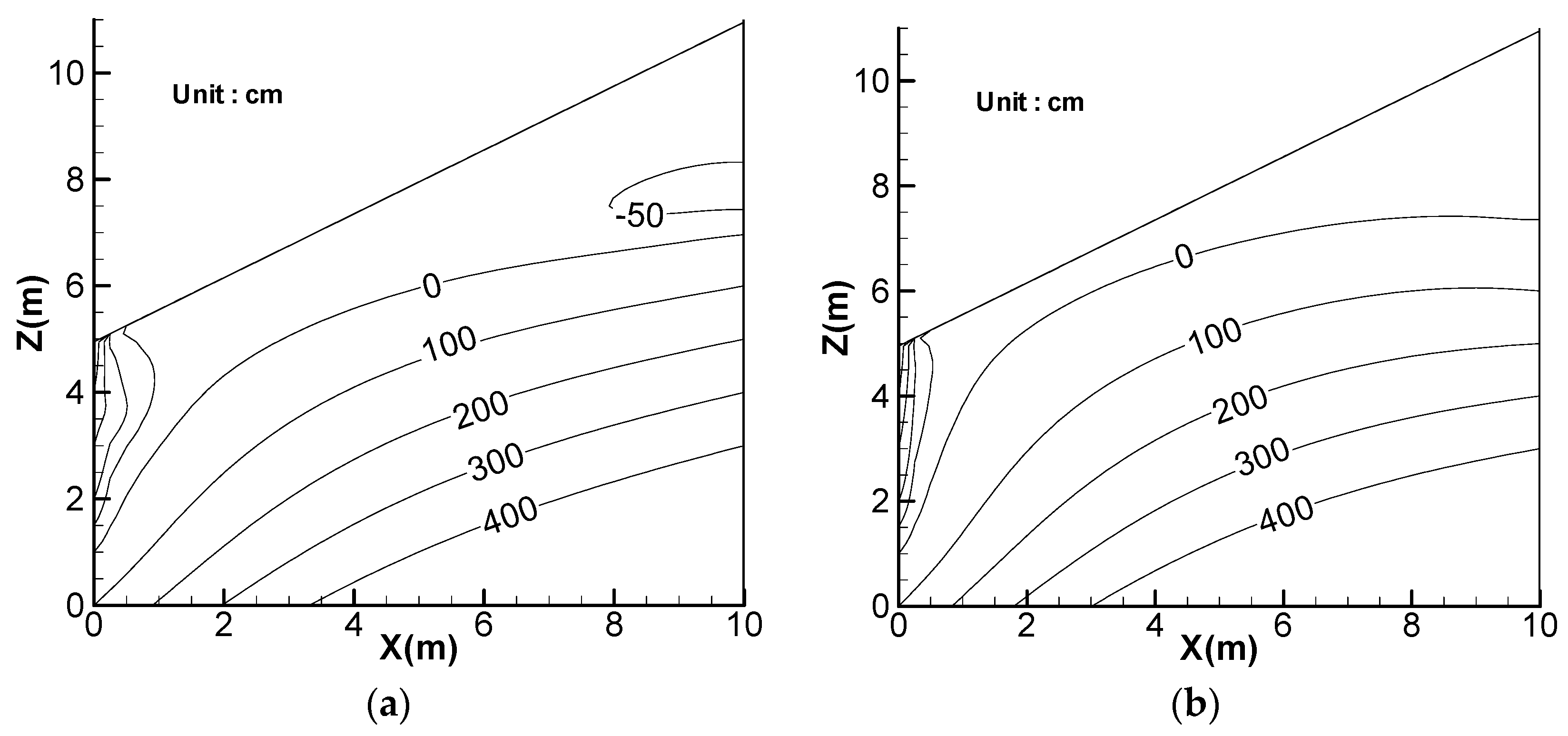
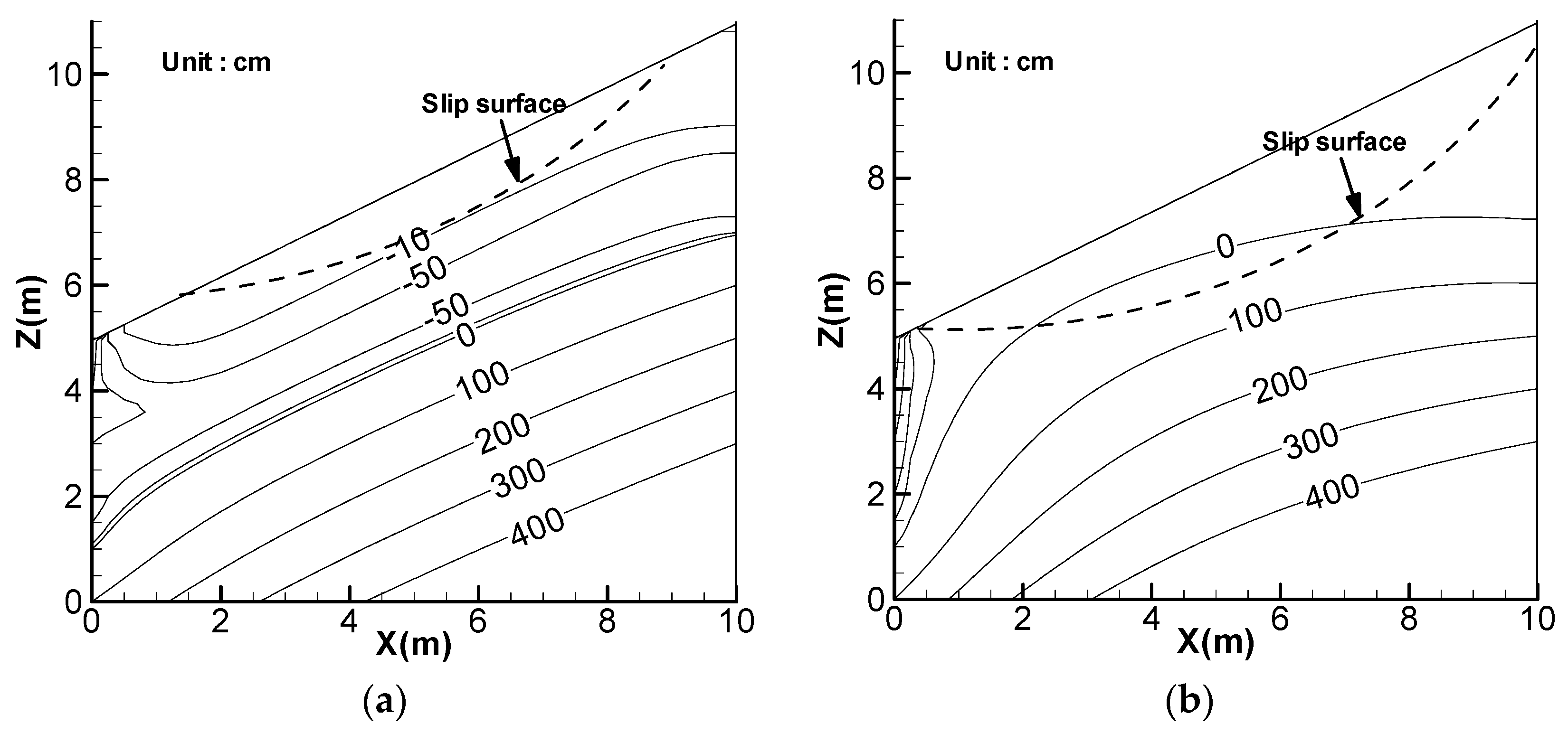
Section 4, Section 5 and Section 6 did not systematically consider the location of the sliding surface, but two-dimensional modeling was necessary to assess the location of a slope surface and the occurrence time of slope failure. As shown in Figure 15, one can find that the location and occurrence time of slope failure were different for different durations under the same rainfall amount with a uniform rainfall pattern. The slip surface partly under the ground water table in saturated soil (Figure 15b) was deeper than the slip surface above the groundwater table in unsaturated soil (Figure 15a). Therefore, the depth of the slip surface is also influenced by the intensity and duration of the rainfall, and the amount of sliding material is not always the same for all the considered scenarios.
8. Conclusions
In this study, a physical-process-based numerical model was developed to reliably assess landslides by using the two-dimensional Richards’ equation and the limit equilibrium slope stability method to simulate local slope instability phenomena. The effects of rainfall and lateral flows on hillslopes were thoroughly analyzed using the proposed approach. The results revealed that slope stability is strongly related to rainfall intensity and duration. The depth of the slip surface is also influenced by the intensity and duration of the rainfall. Under the same duration, higher rainfall intensity was more likely to trigger a slope failure. However, when the amount of rainfall was the same, slope failure may or may not have occurred during various durations. During a specific duration and rainfall amount, the slope instability is influenced by lateral flow caused by the variation in mass flux through the hillslope. The groundwater outflow from the slope boundary may cause great effect during a long rainfall duration. As the lateral flow effects, the anisotropy can also strongly relate to the slope failure. Besides, the effects of rainfall patterns on the slope stability during a specific rainfall duration and at various rainfall amounts were analyzed, but no consistent tendency was observed. However, rainfall patterns play an important role that affects slope stability. Therefore, the threshold curve for each rainfall pattern, developed using the proposed two-dimensional landslide model, revealed the lower and upper bounds of rainfall durations. The results were dissimilar to those obtained using one-dimensional modeling, in which the influence of lateral flow is not considered. Thus, Two-dimensional landslide modeling is necessary because it enables the effect of lateral flow on slope stability to be considered and, thus, provides reliable results.
Author Contributions
H.-E. Chen and T.-L. Tsai built the model; H.-E. Chen, T.-L. Tsai and J.-C. Yang designed the experiments; H.-E. Chen analyzed the data; and H.-E. Chen, T.-L. Tsai and J.-C. Yang wrote the paper.
Conflicts of Interest
The authors declare no conflicts of interest.
References
- Campbell, R. Debris flows originating from soil slips during rainstorms in Southern California. Q. J. Eng. Geol. Hydrogeol. 1974, 7, 339–349. [Google Scholar] [CrossRef]
- Brand, E.W.; Premchitt, J.; Phillipson, H.B. Relationship between rainfall and landslides in Hong Kong. In Proceedings of the Fourth International Symposium on Landslides, Toronto, ON, Canada, 16–21 September 1984; Canadian Geotechnical Society: Richmond, BC, Canada, 1984; pp. 377–384. [Google Scholar]
- Caine, N. The rainfall intensity: Duration control of shallow landslides and debris flows. Geogr. Ann. A 1980, 62, 23–27. [Google Scholar] [CrossRef]
- Cannon, S.H. Rainfall conditions for abundant debris avalanches, San Francisco Bay region, California. Calif. Geol. 1985, 38, 267–272. [Google Scholar]
- Jibson, R.W. Debris flows in Southern Puerto Rico. Geol. Soc. Am. Spec. Pap. 1989, 236, 29–56. [Google Scholar]
- Wieczorek, G.F.; Morgan, B.A.; Campbell, R.H. Debris-flow hazards in the blue ridge of central Virginia. Environ. Eng. Geosci. 2000, 6, 3–23. [Google Scholar] [CrossRef]
- Govi, M.; Mortara, G.; Sorzana, P.F. Eventi idrologici e frane. Geol. Appl. Idrogeol. 1985, 2, 395–401. (In Italian) [Google Scholar]
- Glade, T. Modelling landslide-triggering rainfalls in different regions of New Zealand-The soil water status mode. Z. Geomorphol. Suppl. 2000, 122, 63–84. (In German) [Google Scholar]
- Cai, F.; Ugai, K. Numerical analysis of rainfall effects on slope stability. Int. J. Geomech. 2004, 4, 69–78. [Google Scholar] [CrossRef]
- Gabet, E.J.; Burbank, D.W.; Putkonen, J.K.; Pratt-Sitaula, B.A.; Ojha, T. Rainfall thresholds for landsliding in the Himalayas of Nepal. Geomorphology 2004, 63, 131–143. [Google Scholar] [CrossRef]
- Tsai, T.-L. The influence of rainstorm pattern on shallow landslide. Environ. Geol. 2008, 53, 1563–1569. [Google Scholar] [CrossRef]
- Tsai, T.-L.; Wang, J.-K. Examination of influences of rainfall patterns on shallow landslides due to dissipation of matric suction. Environ. Earth Sci. 2011, 63, 65–75. [Google Scholar] [CrossRef]
- Tarantino, A.; Bosco, G. Role of soil suction in understanding the triggering mechanisms of flow slides associated with rainfall. In Debris-Flow Hazards Mitigation: Mechanics, Prediction, And Assessment, Proceedings of Second International Conference on Debris-Flow Hazards Mitigation, Taipei, Taiwan, 16–18 August 2000; A.A. Balkema: Rotterdam, The Netherlands, 2000; pp. 81–88. [Google Scholar]
- Collins, B.D.; Znidarcic, D. Stability analyses of rainfall induced landslides. J. Geotech. Geoenviron. Eng. 2004, 130, 362–372. [Google Scholar] [CrossRef]
- Tsai, T.-L.; Chen, H.-E.; Yang, J.-C. Numerical modeling of rainstorm-induced shallow landslides in saturated and unsaturated soils. Environ. Geol. 2008, 55, 1269–1277. [Google Scholar] [CrossRef]
- Fredlund, D.G.; Morgenstern, N.R.; Widger, R.A. The shear strength of unsaturated soils. Can. Geotech. J. 1978, 15, 313–321. [Google Scholar] [CrossRef]
- Iverson, R.M. Landslide triggering by rain infiltration. Water Resour. Res. 2000, 36, 1897–1910. [Google Scholar] [CrossRef]
- Baum, R.L.; Savage, W.Z.; Godt, J.W. Trigrs—A Fortran Program for Transient Rainfall Infiltration and Grid-Based Regional Slope-Stability Analysis; version 2.0; U.S. Geological Survey: Reston, VA, USA, 2008.
- Tsai, T.-L.; Yang, J.-C. Modeling of rainfall-triggered shallow landslide. Environ. Geol. 2006, 50, 525–534. [Google Scholar] [CrossRef]
- Van Asch, T.W.J.; Hendriks, M.R.; Hessel, R.; Rappange, F.E. Hydrological triggering conditions of landslides in varved clays in the French Alps. Eng. Geol. 1996, 42, 239–251. [Google Scholar] [CrossRef]
- Crosta, G.; Frattini, P. Distributed modelling of shallow landslides triggered by intense rainfall. Nat. Hazard. Earth Syst. Sci. 2003, 3, 81–93. [Google Scholar] [CrossRef]
- Keim, R.F.; Skaugset, A.E. Modelling effects of forest canopies on slope stability. Hydrol. Process. 2003, 17, 1457–1467. [Google Scholar] [CrossRef]
- Frattini, P.; Crosta, G.B.; Fusi, N.; Dal Negro, P. Shallow landslides in pyroclastic soils: A distributed modelling approach for hazard assessment. Eng. Geol. 2004, 73, 277–295. [Google Scholar] [CrossRef]
- Lan, H.; Lee, C.; Zhou, C.; Martin, C. Dynamic characteristics analysis of shallow landslides in response to rainfall event using GIS. Environ. Geol. 2005, 47, 254–267. [Google Scholar] [CrossRef]
- D’Odorico, P.; Fagherazzi, S.; Rigon, R. Potential for landsliding: Dependence on hyetograph characteristics. J. Geophys. Res. Earth Surf. 2005, 110. [Google Scholar] [CrossRef]
- Conte, E.; Troncone, A. A method for the analysis of soil slips triggered by rainfall. Géotechnique 2012, 62, 187–192. [Google Scholar] [CrossRef]
- Floris, M.; D’Alpaos, A.; Agostini, A.D.; Stevan, G.; Tessari, G.; Genevois, R. A process-based model for the definition of hydrological alert systems in landslide risk mitigation. Nat. Hazard. Earth Syst. Sci. 2012, 12, 3343–3357. [Google Scholar] [CrossRef]
- Conte, E.; Donato, A.; Troncone, A. A simplified method for predicting rainfall-induced mobility of active landslides. Landslides 2017, 14, 35–45. [Google Scholar] [CrossRef]
- Sun, G.; Yang, Y.; Cheng, S.; Zheng, H. Phreatic line calculation and stability analysis of slopes under the combined effect of reservoir water level fluctuations and rainfall. Can. Geotech. J. 2016, 54, 631–645. [Google Scholar] [CrossRef]
- Rahimi, A.; Rahardjo, H.; Leong, E.-C. Effect of antecedent rainfall patterns on rainfall-induced slope failure. J. Geotech. Geoenviron. Eng. 2010, 137, 483–491. [Google Scholar] [CrossRef]
- Richards, L.A. Capillary conduction of liquids through porous mediums. Physics 1931, 1, 318–333. [Google Scholar] [CrossRef]
- Van Genuchten, M.T. A closed-form equation for predicting the hydraulic conductivity of unsaturated soils. Soil Sci. Soc. Am. J. 1980, 44, 892–898. [Google Scholar] [CrossRef]
- Bishop, A.W. The use of pore-pressure coefficients in practice. Geotechnique 1954, 4, 148–152. [Google Scholar] [CrossRef]
- Celia, M.A.; Bouloutas, E.T.; Zarba, R.L. A general mass-conservative numerical solution for the unsaturated flow equation. Water Resour. Res. 1990, 26, 1483–1496. [Google Scholar] [CrossRef]
Figure 1.
Slope of Bishop slip circle.

Figure 2.
Flow chart for computational procedure.

Figure 3.
Geometry of modeling slope.

Figure 4.
Factor of safety for various duration with uniform rainfall of: (a) 300 mm; (b) 400 mm; and (c) 500 mm.
Figure 4.
Factor of safety for various duration with uniform rainfall of: (a) 300 mm; (b) 400 mm; and (c) 500 mm.

Figure 5.
Pressure head contours for duration of 24 h with uniform rainfall of 400 mm at time: (a) 12 h; (b) 24 h; and (c) 36 h.
Figure 5.
Pressure head contours for duration of 24 h with uniform rainfall of 400 mm at time: (a) 12 h; (b) 24 h; and (c) 36 h.
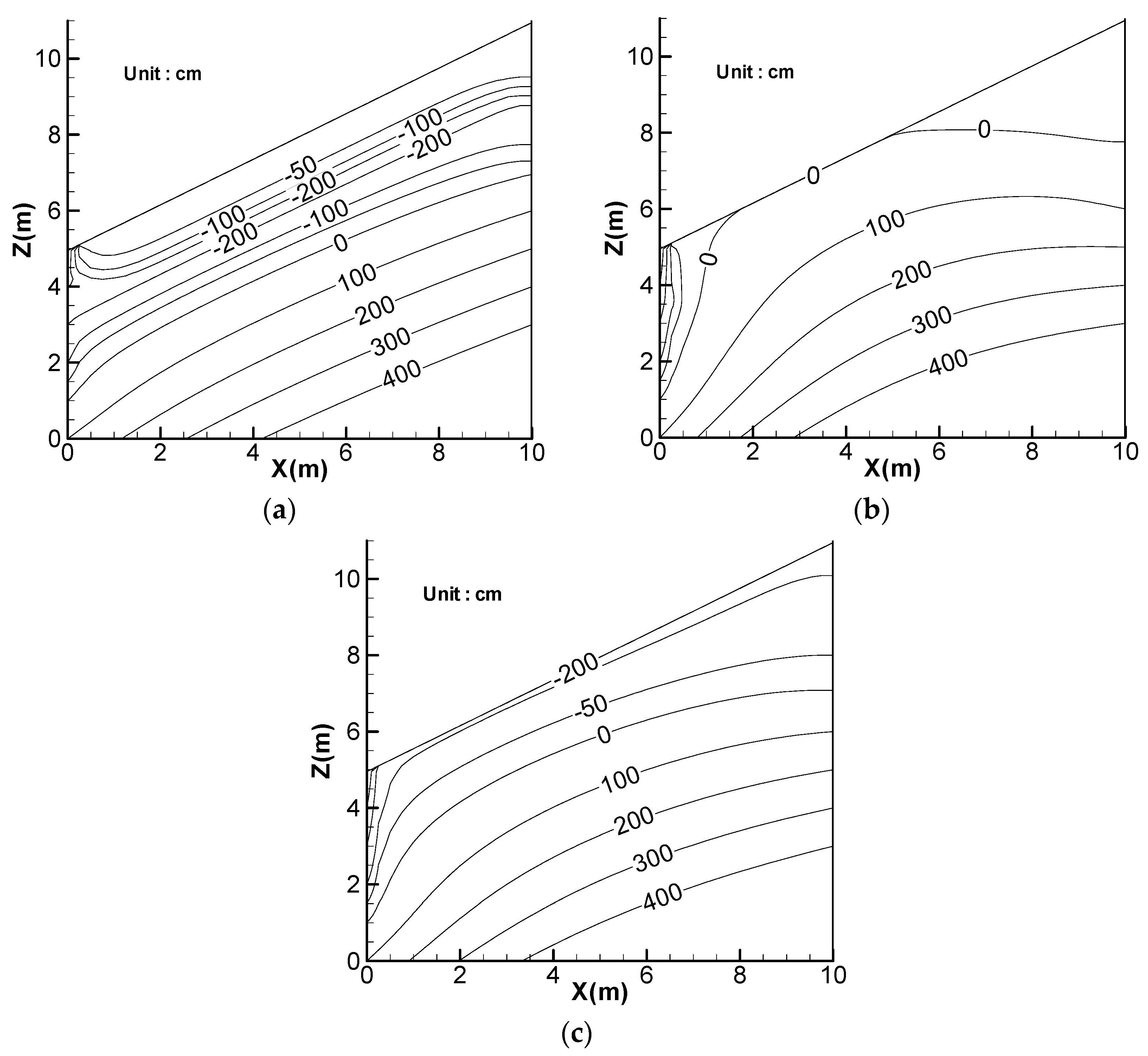
Figure 6.
Pressure head contours for duration of 36 h with uniform rainfall of 500 mm at time: (a) 12 h; (b) 26.5 h; (c) 34 h; (d) 36 h; and (e) 48 h.
Figure 6.
Pressure head contours for duration of 36 h with uniform rainfall of 500 mm at time: (a) 12 h; (b) 26.5 h; (c) 34 h; (d) 36 h; and (e) 48 h.

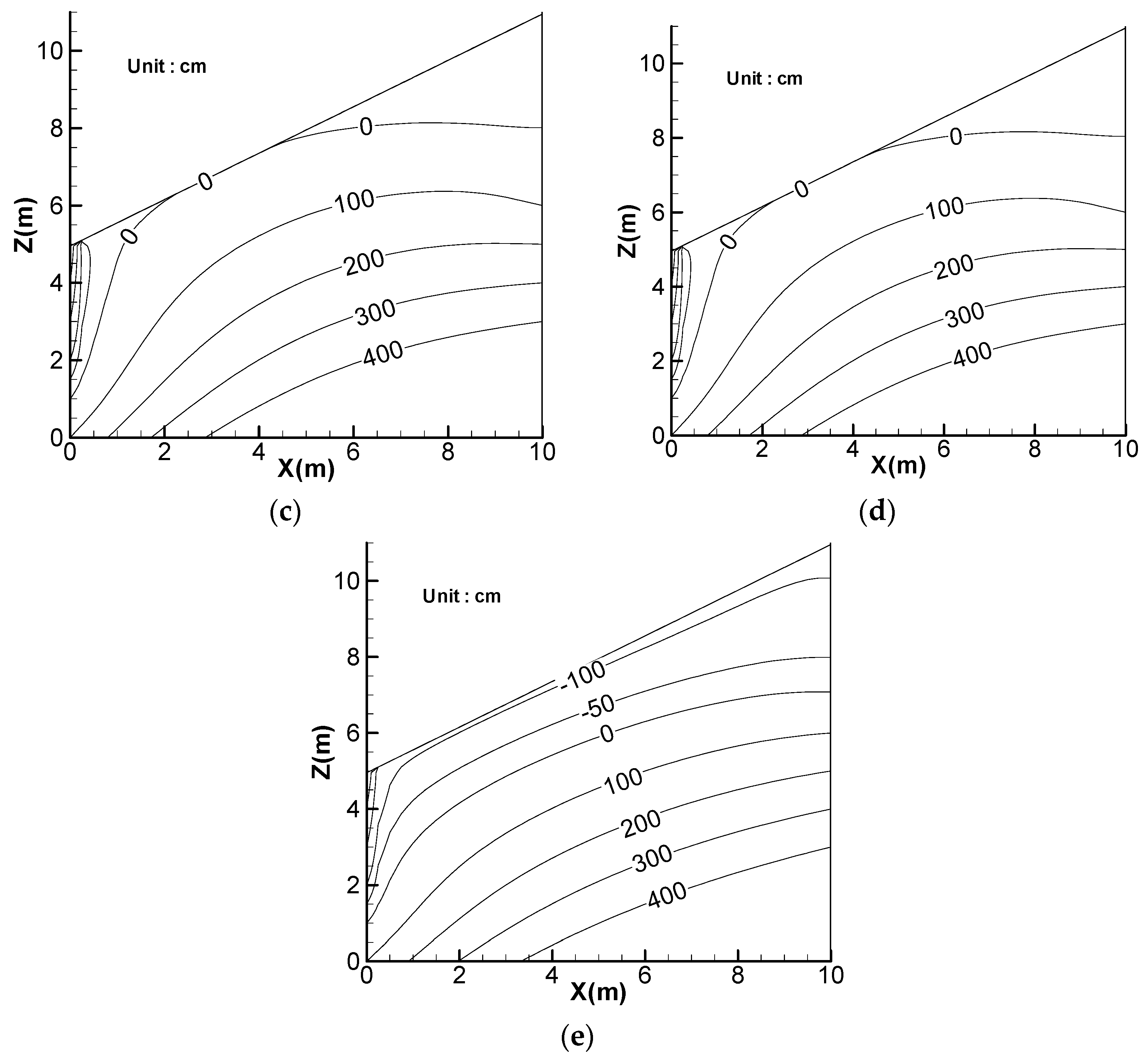
Figure 7.
Slope surface inflow (a); and mass added (b) for different duration with uniform rainfall of 400 mm.
Figure 7.
Slope surface inflow (a); and mass added (b) for different duration with uniform rainfall of 400 mm.
Figure 8.
Pressure head contours for duration of 6 h with uniform rainfall of 400 mm at time: (a) 3 h; and (b) 6 h.
Figure 8.
Pressure head contours for duration of 6 h with uniform rainfall of 400 mm at time: (a) 3 h; and (b) 6 h.
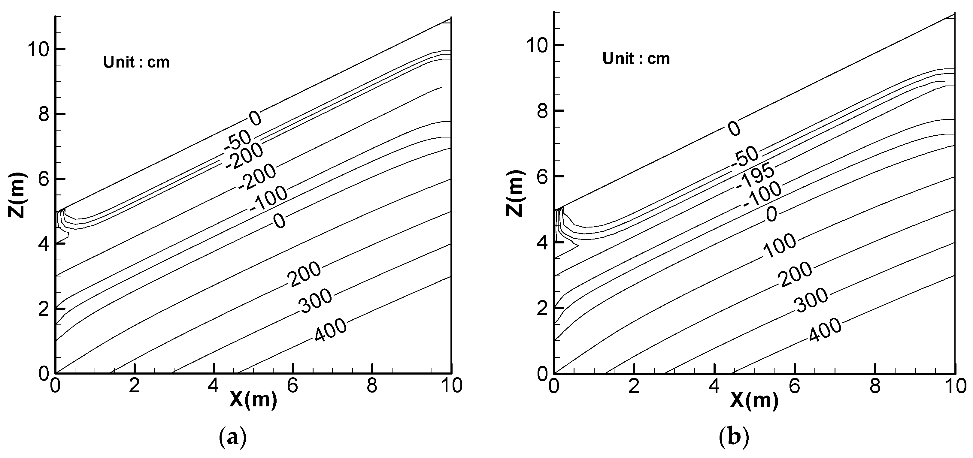
Figure 9.
Pressure head contours for duration of 12 h with uniform rainfall of 400 mm at time: (a) 6 h; and (b) 12 h.
Figure 9.
Pressure head contours for duration of 12 h with uniform rainfall of 400 mm at time: (a) 6 h; and (b) 12 h.

Figure 10.
Pressure head contours for duration of 36 h with uniform rainfall of 400 mm at time: (a) 30 h; and (b) 36 h.
Figure 10.
Pressure head contours for duration of 36 h with uniform rainfall of 400 mm at time: (a) 30 h; and (b) 36 h.

Figure 11.
Pressure head contours for duration of 48 h with uniform rainfall of 400 mm at time: (a) 40 h; and (b) 48 h.
Figure 11.
Pressure head contours for duration of 48 h with uniform rainfall of 400 mm at time: (a) 40 h; and (b) 48 h.
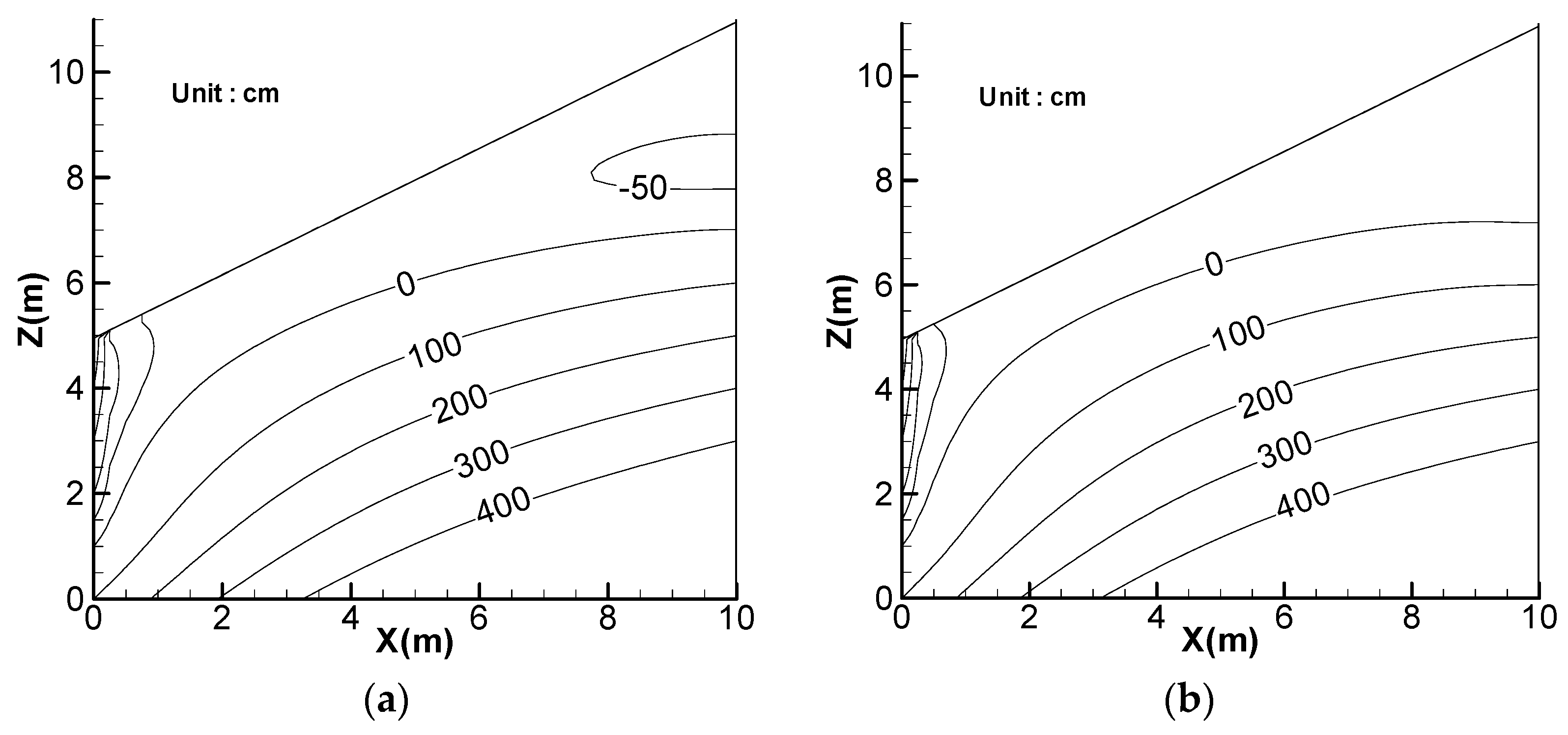
Figure 12.
The four representative rainfall patterns [11].
Figure 12.
The four representative rainfall patterns [11].

Figure 13.
Factor of safety for various durations of 400 mm rainfall with rainfall patterns of: (a) advanced rainfall; (b) intermediate rainfall; and (c) delayed rainfall.
Figure 13.
Factor of safety for various durations of 400 mm rainfall with rainfall patterns of: (a) advanced rainfall; (b) intermediate rainfall; and (c) delayed rainfall.
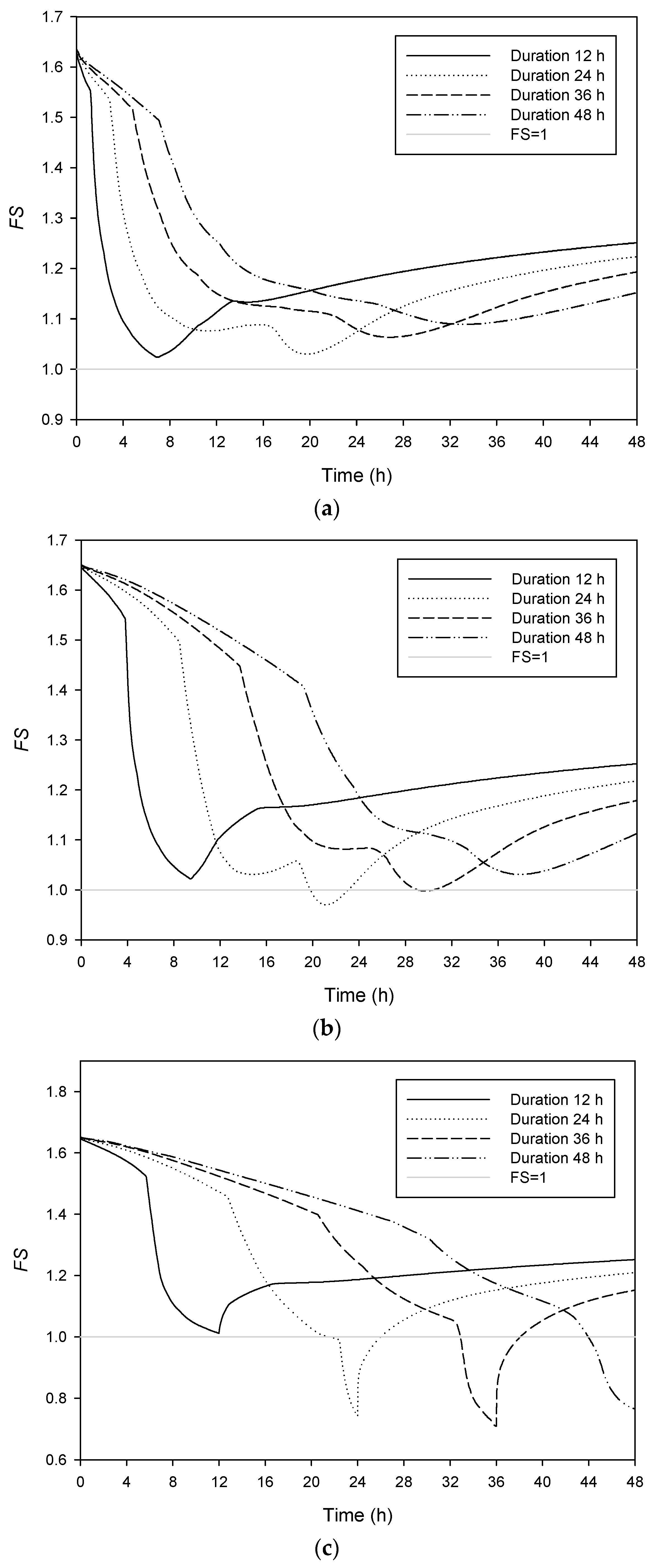
Figure 14.
Threshold of slope instability induced by rainfall and lateral flow.

Figure 15.
Pressure head contours and slip surface with uniform rainfall of 400 mm for duration of: (a) 12 h; and (b) 36 h.
Figure 15.
Pressure head contours and slip surface with uniform rainfall of 400 mm for duration of: (a) 12 h; and (b) 36 h.
© 2017 by the authors. Licensee MDPI, Basel, Switzerland. This article is an open access article distributed under the terms and conditions of the Creative Commons Attribution (CC BY) license (http://creativecommons.org/licenses/by/4.0/).
Share and Cite
MDPI and ACS Style
Chen, H.-E.; Tsai, T.-L.; Yang, J.-C. Threshold of Slope Instability Induced by Rainfall and Lateral Flow. Water 2017, 9, 722. https://doi.org/10.3390/w9090722
AMA Style
Chen H-E, Tsai T-L, Yang J-C. Threshold of Slope Instability Induced by Rainfall and Lateral Flow. Water. 2017; 9(9):722. https://doi.org/10.3390/w9090722
Chicago/Turabian StyleChen, Hung-En, Tung-Lin Tsai, and Jinn-Chuang Yang. 2017. "Threshold of Slope Instability Induced by Rainfall and Lateral Flow" Water 9, no. 9: 722. https://doi.org/10.3390/w9090722
Note that from the first issue of 2016, this journal uses article numbers instead of page numbers. See further details here.