Multivariate Analysis of Rangeland Vegetation and Soil Organic Carbon Describes Degradation, Informs Restoration and Conservation

Abstract

Agricultural expansion has eliminated a high proportion of native land cover and severely degraded remaining native vegetation. Managers must determine where degradation is severe enough to merit restoration action, and what action, if any, is necessary. We report on grassland degraded by multiple factors, including grazing, soil disturbance, and exotic plant species introduced in response to agriculture management. We use a multivariate method to categorize plant communities by degradation state based on floristic and biophysical degradation associated with historical land use. The variables we associate with degradation include abundance of the invasive cool-season grass, tall fescue (Schedonorus phoenix (Scop.) Holub); soil organic carbon (SOC); and heavy livestock grazing. Using a series of multivariate analyses (ordination, hierarchical clustering, and multiple regression), we identify patterns in plant community composition and describe floristic degradation states. We found vegetation states to be described largely by vegetation composition associated primarily with tall fescue and secondarily by severe grazing, but not soil organic carbon. Categorizing grasslands by vegetation states helps managers efficiently apply restoration inputs that optimize ecosystem response, so we discuss potential restoration pathways in a state-and-transition model. Reducing stocking rate on grassland where grazing is actively practiced is an important first step that might be sufficient for restoring grassland with high native species richness and minimal degradation from invasive plants. More severe degradation likely requires multiple approaches to reverse degradation. Of these, we recommend restoration of ecological processes and disturbance regimes such as fire and grazing. We suggest old-field grasslands in North America, which are similar to European semi-natural grassland in composition and function, deserve more attention by conservation biologists.

1. Introduction

Anthropogenic impacts have been documented across more than three-quarters of the Earth’s ice-free terrestrial surface [1,2], and the global intensification of land use threatens biodiversity in human-impacted areas [3,4]. Multifunctional landscapes comprised of natural and semi-natural ecosystems set in the context of intensive land use can address multiple goals of production and conservation [5,6,7], but severe degradation can overcome ecosystem resilience and reduce ecosystem stability and function through catastrophic state shifts [8].

In degraded environments, conservation of native biodiversity and restoration of ecosystem function often requires some degree of ecosystem restoration to a less-degraded state. As such, managers must often determine the causes of ecological degradation before proceeding with restoration. When degradation factors are clear and controllable, restoration can be managed agronomically and proceeds linearly towards a restoration objective, such as pre-settlement conditions [9]. For example, restoring native grassland from cropland agriculture typically involves managing for maximal native species diversity and minimal non-native species by planting a diverse mix of native species and removing exotic species [10,11].

Restoration of intensively cultivated areas is fairly straightforward, but the best course of restoration action for sites degraded by multiple factors can be elusive. Specific sources of degradation might not be readily identifiable because they result from multiple causative factors that vary spatially and temporally, and the response to restoration might be non-linear and unpredictable [12,13,14]. Land-use history, recent disturbance, and invasive species create legacies with long-term impacts on plant community composition that strongly resist change toward the desired restoration outcome [12,15,16]. Restoration and conservation under such conditions require an ecological approach using the initial extent of floristic degradation to identify appropriate restoration action and outcomes [9,17].

We construct vegetation states to describe floristic degradation in nine old-field grassland tracts in south-central Iowa and north-central Missouri, USA. This study was prompted by a clear need to identify patterns of floristic degradation that influence other taxa in these grasslands [18,19,20]. We use multivariate analyses to categorize floristic degradation into vegetation states with plant species data, a common approach in rangelands worldwide [21,22,23]. We also use soil organic carbon (SOC) as an indicator of biophysical degradation because both cultivation and severe grazing have been shown to reduce SOC content [24].

We report the relationship between native and exotic plant species abundance, grazing history, and a regionally-ubiquitous invasive plant species, the Eurasian, cool-season grass, tall fescue (Schedonorus phoenix (Scop.) Holub). Tall fescue is one of the most economically-important grasses in eastern North America since its introduction in the 1940’s [25], but tall fescue has since been shown to reduce native plant species richness, fire spread, and habitat quality in grassland [26,27,28,29,30].

We predicted that patterns of plant community composition (i.e., vegetation states) correspond to patterns in three factors of degradation: tall fescue abundance, grazing history and soil organic carbon. To inform restoration action, we use a state-and-transition framework [31,32] to discuss potential degradation and restoration pathways with respect to conservation in working grassland landscapes.

2. Experimental Section

2.1. Study Area

2.1.1. Environment and Soils

Our study was located in a 30,000 ha tallgrass prairie ecosystem spanning Ringgold County, Iowa, and Harrison County, Missouri, USA known as the Grand River Grasslands. Long-term mean annual rainfall is 91 cm; mean January and July temperatures are −6 °C and 24 °C, respectively [33]. Soils of the study area belong to the Gara-Armstrong-Pershing association, which the Soil Survey of Ringgold County, IA ([34]; p. 10) describes as “gently sloping to steep, well drained to somewhat poorly drained, loamy and silty soils formed in glacial till, a paleosol derived from glacial till, and loess; on uplands and stream benches.” Tracts were dominated by two soil types, Gara loam (Fine-loamy, mixed, superactive, mesic Mollic Hapludalfs) and Armstrong loam (fine, smectitic, mesic Aquertic Hapludalfs), with slopes ranging from 9 to 25 percent and 5 to 14 percent, respectively [35].

2.1.2. Current and Historical Land Use

The Grand River Grasslands have been identified as the best known opportunity to restore a functional tallgrass prairie system in the Central Tallgrass Prairie ecoregion of North America, but only 11% of the GRG is in some form of conservation reserve (The Nature Conservancy, unpublished data). The Grand River Grasslands are a working landscape in which researchers work to reconcile multiple functions including agricultural production, ecosystem function, and biodiversity conservation [36].

We selected nine grassland tracts (15–31 ha) identified by The Nature Conservancy as moderate to high in conservation value, based on the presence of clusters of native prairie species (The Nature Conservancy, unpublished data). Although the conservation value was assigned at the tract level, evidence suggested that land-use history—and thus floristic and biophysical condition—might vary within each tract as well as between tracts. For example, each tract was clearly in a perennial grassland state, but composition appeared to vary in the relative dominance of native and exotic species [37]. Furthermore, the sources of exotic plants are unknown, e.g., whether species were intentionally sown, either at the tract or landscape scales, and if not, at what spatial and temporal scales encroachment occurred. As such, we expected to observe a range of degradation within tracts and among tracts.

Grazing history was determined by interviewing current and previous landowners and managers who reported that four tracts were grazed by cattle during the growing season (May through October) at stocking rates up to 15 animal unit months/ha within five years prior to our study. We applied the category “historically severely grazed” to these four sites, and the category “historically ungrazed” to the remaining five sites [38]. We also queried previous landowners and managers about cultivation history and reviewed available aerial imagery of the tracts beginning in the 1930s and extending through the study period. Although no evidence of cultivation was reported or observed, we cannot rule out that some areas of some tracts were farmed for brief periods following European settlement.

2.2. Sampling

We established six permanent modified Whittaker plots [39] per tract to sample presence and abundance of vascular plant species. Plot locations were selected at random within each of the two most dominant soil types (three plots on each soil type) via GIS to control for catena and distance from edges to ensure similar landscape position and minimal edge effects among plots across all tracts. All tracts were relatively high on the landscape.

Within modified Whittaker plots, sampling occurred at four different scales: 0.5 m², 2.5 m², 250 m², and 500 m². Abundance (canopy cover of individual species) was sampled within 10 0.5-m² quadrats, indexed by the Daubenmire [40] canopy cover index. Sedges (Cyperaceae) were identified to family. In plots larger than 0.5 m², only species presence was recorded. For purposes of analyses, species found outside of the 10 quadrats but within the 500 m² plot were assigned a cover value of 0.01. Sampling occurred twice during the growing season—once in late May-early June and again in August 2006—to account for plant growth and senescence and therefore community change through the growing season. The maximum canopy cover value of each species across both sampling periods was used in analyses.

To measure soil degradation within the modified Whittaker plots, we use soil organic carbon (SOC) depletion because SOC declines with cultivation and similarly-intense disturbances (e.g., severe grazing) that substantially disturb the vegetation matrix and soil [24,41,42,43]. Each modified Whittaker plot was represented by a composite soil sample created by combining four 15-cm cores taken from each corner of the 500-m² plot. Samples were analyzed for pH (soil slurry method) and total carbon by volume (loss on ignition method). Correction for inorganic carbon content was unnecessary because pH of all samples was ≤7.0. To contextualize our soil organic carbon data, we compared our SOC values to regional data taken from cultivated fields of the same soil types available online from the National Cooperative Soil Survey [44].

2.3. Data Analysis

2.3.1. Patterns of Degradation

We associated plant community composition with potential sources of degradation—SOC, grazing history, and invasive species—using the ordination technique Non-metric Multidimensional Scaling (NMDS) [45]. We chose the Canberra distance measure for our NMDS distance matrix, which ranges from zero (identical community composition) to one (complete dissimilarity) for its sensitivity to rare species [46]. We also used the Canberra distance matrix to calculate community dissimilarity among individual plots, tracts, and tracts grouped by historical grazing severity. These analyses were performed with the metaMDS and vegdist functions, respectively, in the VEGAN package for program R [47,48,49]. To minimize stress, the NMDS was projected in k = 4 dimensions.

Because it is a degradation factor in this study, tall fescue was excluded from the plant community data used in the NMDS. We plotted a smooth surface over the first two dimensions of the NMDS projection [47] to evaluate the association between tall fescue canopy cover and variation in plant community composition. We also calculated the correlation between the ordination and measures of plant community composition (total species richness, exotic and native species abundance, and proportion of native species richness) and compared these richness and abundance data across the historically severely grazed and ungrazed subgroups via Student’s t-tests assuming unequal variance.

2.3.2. Sources of Degradation

We tested the effect of degradation factors on plant community composition with a full-interaction, Multivariate Analysis of Variance (MANOVA) model with the manova function in R, after determining no collinearity existed among the predictor variables. Tall fescue canopy cover, SOC, and grazing history were predictor variables, and scores for all four NMDS axes were used as co-dependent response variables (e.g., [50]). The model ranked independent variables in terms of their relative importance to the model with F statistics approximated by Wilks’ lambda.

2.3.3. Vegetation States

To group plant composition data from modified Whittaker plots, we used hierarchical clustering of the full plant community dataset, including tall fescue. Hierarchical clustering (R function hclust) calculated dissimilarity in plant community composition based on the Canberra distance matrix, from which four groups were discernibly distinct using the R function cutree. Post-hoc analysis indicated that plant communities of two of the four groups identified by the cutree function were similar in abundance of tall fescue, native species richness, total species richness, or proportion native species cover in pair-wise student’s t-tests (p > 0.10). Therefore, we consolidated these two groups into a single vegetation state for subsequent analyses (Appendix Figure A1).

To determine distinctiveness of the three vegetation states in terms of plant community composition, we tested for dissimilarity in plant community composition among vegetation states with the adonis function in the VEGAN package [48]. We also identified the degradation factors and plant community variables that were associated with differences among vegetation states. We began by fitting a linear mixed-effect regression model (LME) in which vegetation state was tested as a response variable against the following predictor variables: tall fescue abundance, grazing history, proportion native species abundance, and Simpson’s diversity (1/D). We accomplished this with the lme function in the nlme package for program R [51]. We then used the stepwise model selection function stepAIC in R to identify variables associated with vegetation state. The stepAIC function removes and re-combines predictor variables from the initial LME model and returns the model with the lowest Akaike’s An Information Criterion (AIC); the minimal AIC value indicates the most parsimonious model likely to best explain variation in the response variable [52]. Finally, to confirm the unique identity of the three plant communities from each other (i.e., the states), we compared the three states for tall fescue abundance, native species richness, total species richness, proportion native species cover and Simpson’s diversity index (1/D) with pair-wise student’s t-tests.

3. Results

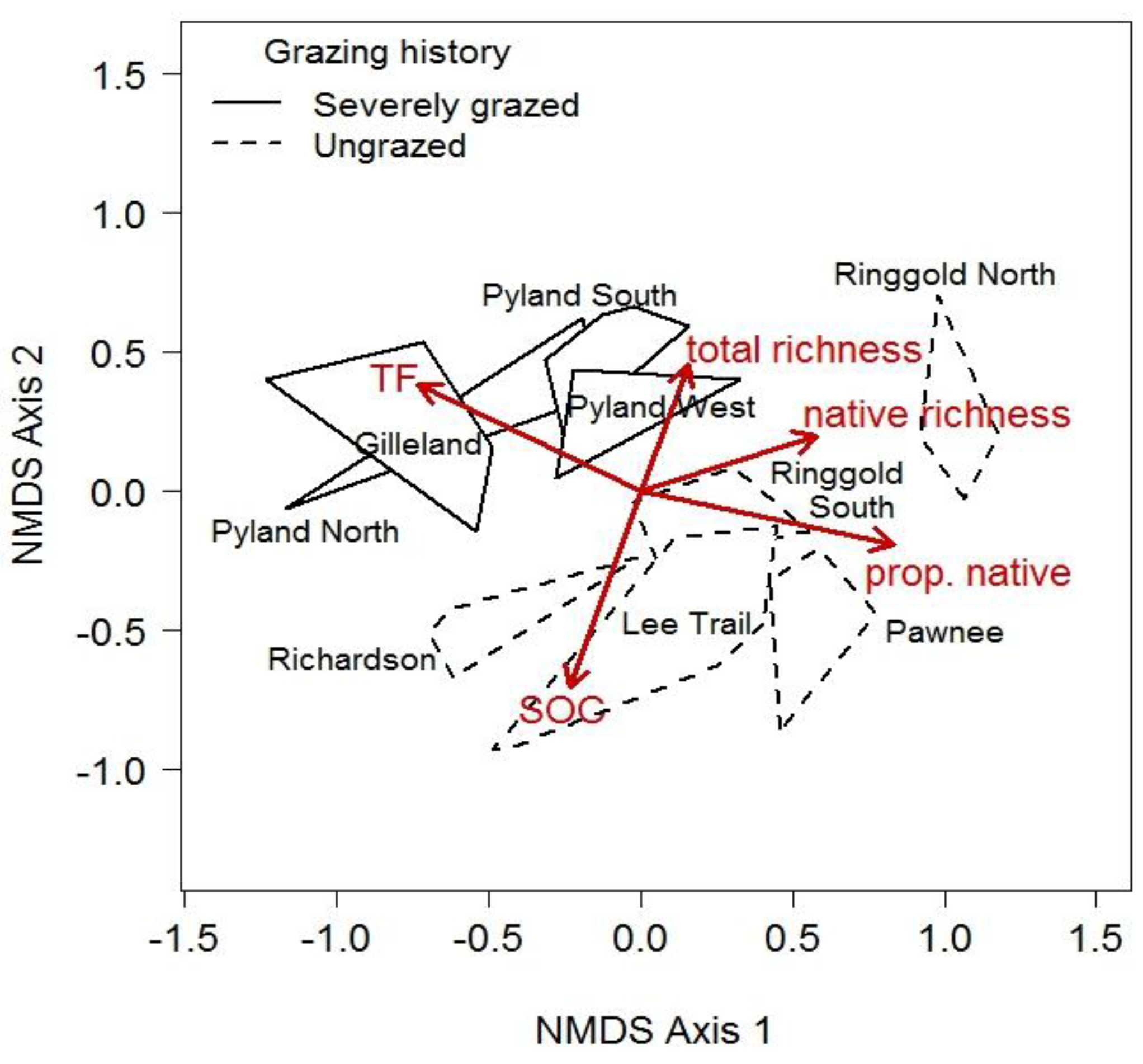
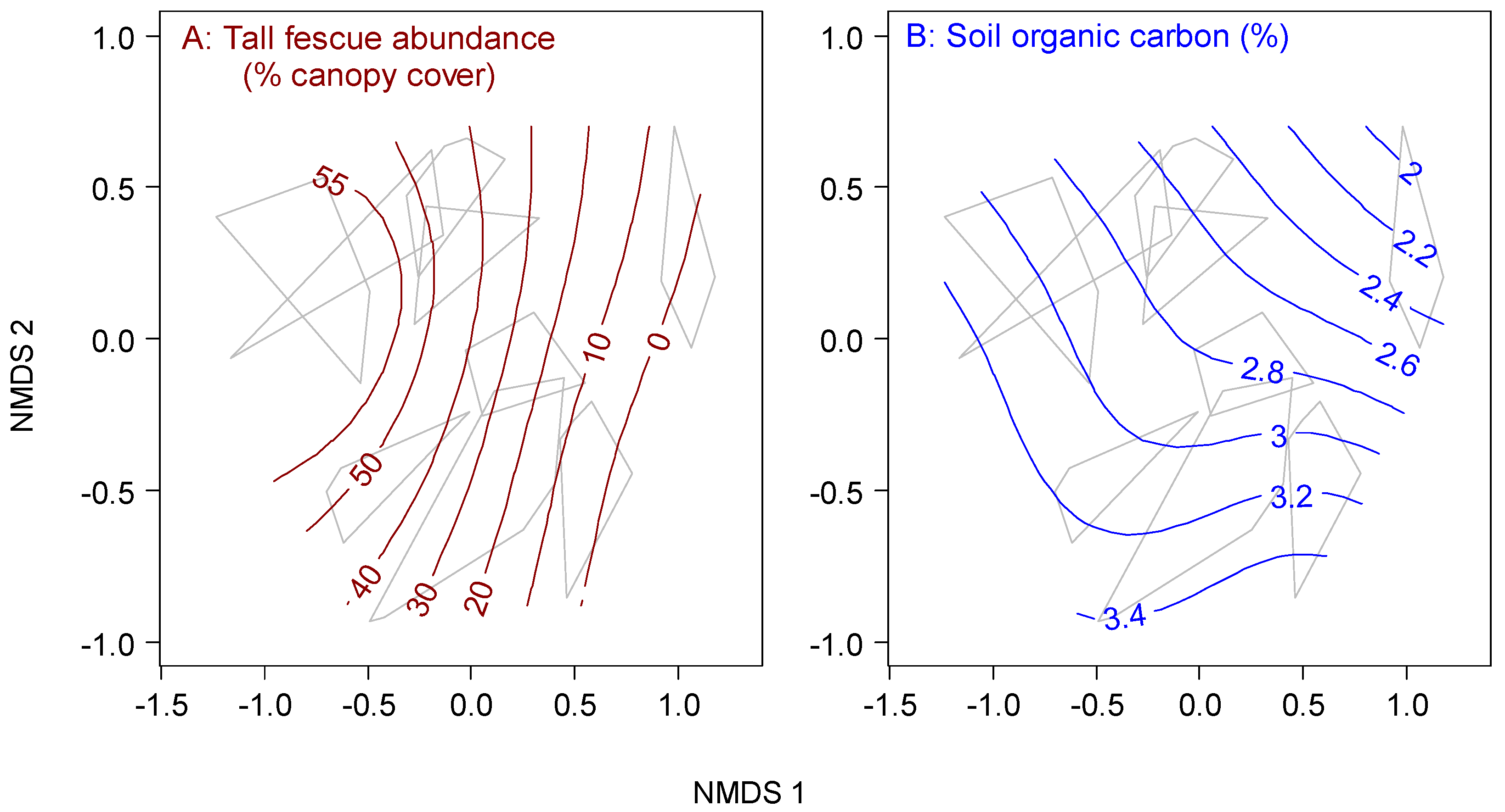
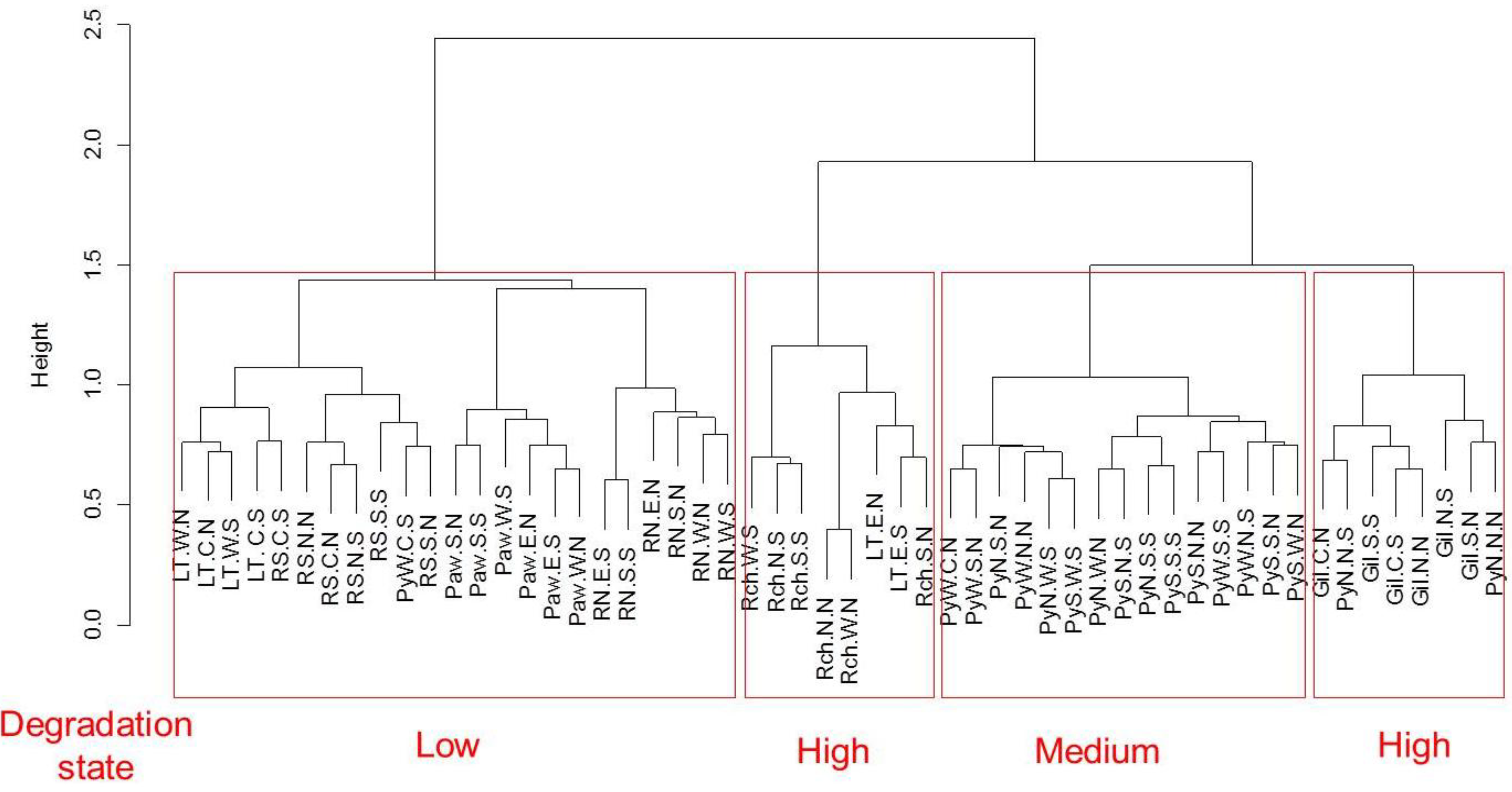
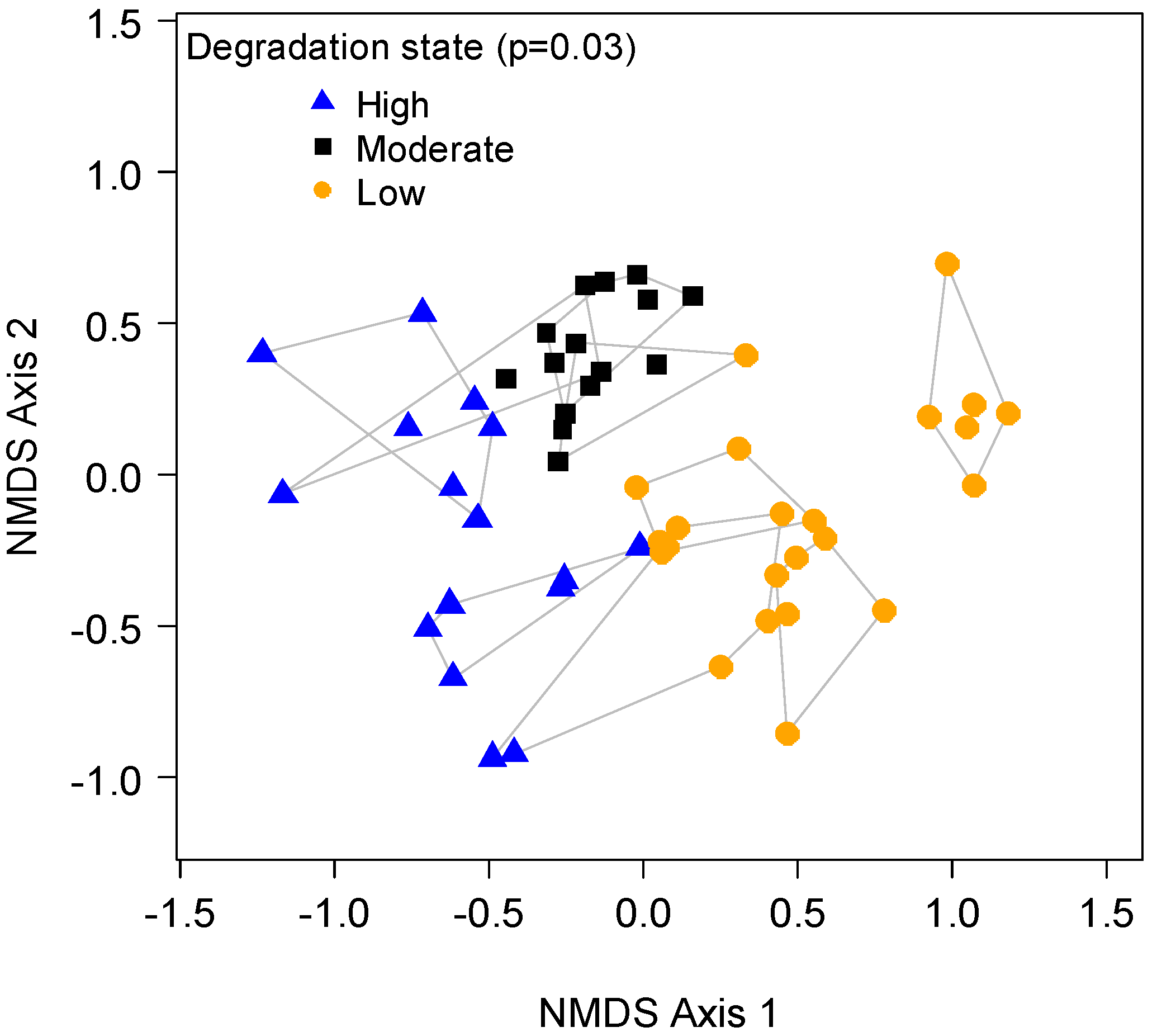
3.1. Pattern of Vegetation Degradation

The nine study tracts contained diverse assemblages of both native and exotic species, but tall fescue was the most frequently-occurring and most abundant plant on most tracts. Only Kentucky bluegrass (Poa pratensis L.) was observed more frequently (49 vs. 43 out of 54 Whittaker plots, respectively), but mean canopy cover of Kentucky bluegrass was less than that of tall fescue (12% ± 2% s.e. vs. 38% ± 3% s.e., respectively). All Whittaker plots contained exotic species, although several were dominated by native species (Table 1). We observed 196 species across 51 dicot families and 3 grass subfamilies, in addition to sedges. We observed 129 flowering herbaceous (forb) species, 14 legumes, 18 warm-season grasses, 18 woody species, and 14 cool-season grasses. Seventy-one percent of the species were native.

Table 1. Ten most abundant species (percent of total canopy cover) within each of three vegetation degradation states identified by hierarchical clustering of 196 plant species abundance sampled from nine tracts in the Grand River Grasslands of south-central Iowa and north-central Missouri, USA.

Vegetation Degradation State	Scientific Name	Common Name	Status	Mean Relative Abundance (%) ±95% CI
High	Schedonorus phoenix	Tall fescue	Exotic	41 ± 5
	Poa pratensis	Kentucky bluegrass	Exotic	20 ± 5
	Bromus inermis	Smooth brome	Exotic	11 ± 6
	Veronia baldwinii	Baldwin’s ironweed	Native	6 ± 4
	Setaria pumila	Yellow foxtail	Exotic	3 ± 4
	Solanum carolinense	Horse nettle	Native	2 ± 2
	Daucus carota	Wild carrot	Exotic	2± 1
	Dactylis glomerata	Orchardgrass	Exotic	2± 1
	Medicago lupulina	Black medic	Exotic	1± 1
	Solidago canadensis	Tall goldenrod	Native	1± 1
			N = 3, E = 7	Sum = 89
Moderate	Schedonorus phoenix	Tall fescue	Exotic	30 ± 4
	Medicago lupulina	Black medic	Exotic	14 ± 4
	Sporobolus clandestinus	Rough dropseed	Native	12 ± 3
	Kummerowia striata	Japanese clover	Exotic	7 ± 4
	Poa pratensis	Kentucky bluegrass	Exotic	6 ± 2
	Aristida oligantha	Prairie threeawn	Native	5 ± 3
	Lotus corniculatus	Birdsfoot trefoil	Exotic	4 ± 4
	Daucus carota	Wild carrot	Exotic	3 ± 1
	Dichanthelium oligosanthes	Scribner’s rosette grass	Native	2 ± 1
	Phleum pratense	Timothy	Exotic	2 ± 1
			N = 3, E = 7	Sum = 83
Low	Sorghastrum nutans	Indiangrass	Native	11 ± 6
	Schedonorus phoenix	Tall fescue	Exotic	9 ± 5
	Cyperaceae	Sedges	Native	9 ± 2
	Andropogon gerardii	Big bluestem	Native	9 ± 5
	Sporobolus clandestinus	Rough dropseed	Native	7 ± 2
	Lotus corniculatus	Birdsfoot trefoil	Exotic	6 ± 4
	Poa pratensis	Kentucky bluegrass	Exotic	6 ± 2
	Solidago canadensis	Tall goldenrod	Native	6 ± 4
	Symphoricarpos orbiculatus	Coralberry	Native	4 ± 3
	Schizachyrium scoparium	Little bluestem	Native	4 ± 3
			N = 7, E = 3	Sum = 71

Table 1. Ten most abundant species (percent of total canopy cover) within each of three vegetation degradation states identified by hierarchical clustering of 196 plant species abundance sampled from nine tracts in the Grand River Grasslands of south-central Iowa and north-central Missouri, USA.

Vegetation Degradation State	Scientific Name	Common Name	Status	Mean Relative Abundance (%) ±95% CI
High	Schedonorus phoenix	Tall fescue	Exotic	41 ± 5
	Poa pratensis	Kentucky bluegrass	Exotic	20 ± 5
	Bromus inermis	Smooth brome	Exotic	11 ± 6
	Veronia baldwinii	Baldwin’s ironweed	Native	6 ± 4
	Setaria pumila	Yellow foxtail	Exotic	3 ± 4
	Solanum carolinense	Horse nettle	Native	2 ± 2
	Daucus carota	Wild carrot	Exotic	2± 1
	Dactylis glomerata	Orchardgrass	Exotic	2± 1
	Medicago lupulina	Black medic	Exotic	1± 1
	Solidago canadensis	Tall goldenrod	Native	1± 1
			N = 3, E = 7	Sum = 89
Moderate	Schedonorus phoenix	Tall fescue	Exotic	30 ± 4
	Medicago lupulina	Black medic	Exotic	14 ± 4
	Sporobolus clandestinus	Rough dropseed	Native	12 ± 3
	Kummerowia striata	Japanese clover	Exotic	7 ± 4
	Poa pratensis	Kentucky bluegrass	Exotic	6 ± 2
	Aristida oligantha	Prairie threeawn	Native	5 ± 3
	Lotus corniculatus	Birdsfoot trefoil	Exotic	4 ± 4
	Daucus carota	Wild carrot	Exotic	3 ± 1
	Dichanthelium oligosanthes	Scribner’s rosette grass	Native	2 ± 1
	Phleum pratense	Timothy	Exotic	2 ± 1
			N = 3, E = 7	Sum = 83
Low	Sorghastrum nutans	Indiangrass	Native	11 ± 6
	Schedonorus phoenix	Tall fescue	Exotic	9 ± 5
	Cyperaceae	Sedges	Native	9 ± 2
	Andropogon gerardii	Big bluestem	Native	9 ± 5
	Sporobolus clandestinus	Rough dropseed	Native	7 ± 2
	Lotus corniculatus	Birdsfoot trefoil	Exotic	6 ± 4
	Poa pratensis	Kentucky bluegrass	Exotic	6 ± 2
	Solidago canadensis	Tall goldenrod	Native	6 ± 4
	Symphoricarpos orbiculatus	Coralberry	Native	4 ± 3
	Schizachyrium scoparium	Little bluestem	Native	4 ± 3
			N = 7, E = 3	Sum = 71

Figure 1. Ordination of plant species composition from 54 modified Whittaker plots (plots) by Nonmetric Multi-Dimensional Scaling (NMDS) of Canberra distances (k = 4, stress ≈ 12%). The ordination is based on 196 plant species abundance sampled from nine tracts in the Grand River Grasslands of south-central Iowa and north-central Missouri, USA. Plant communities are plotted by tract and grazing history. The six Whittaker plots of each tract are connected by minimum convex hulls in which unbroken lines denote tracts with a recent history of severe grazing, and broken lines denote tracts with no recent history of grazing. Arrows indicate vectors of increase along a gradient of variation within ordination space for each factor. Arrow length is proportional to the correlation between a variable and the NMDS axis closest to parallel with the vector. Vector abbreviations: TF = tall fescue abundance, prop. native = proportion of native species abundance, native rich = native species richness, total rich = total species richness, SOC = soil organic carbon.

Figure 1. Ordination of plant species composition from 54 modified Whittaker plots (plots) by Nonmetric Multi-Dimensional Scaling (NMDS) of Canberra distances (k = 4, stress ≈ 12%). The ordination is based on 196 plant species abundance sampled from nine tracts in the Grand River Grasslands of south-central Iowa and north-central Missouri, USA. Plant communities are plotted by tract and grazing history. The six Whittaker plots of each tract are connected by minimum convex hulls in which unbroken lines denote tracts with a recent history of severe grazing, and broken lines denote tracts with no recent history of grazing. Arrows indicate vectors of increase along a gradient of variation within ordination space for each factor. Arrow length is proportional to the correlation between a variable and the NMDS axis closest to parallel with the vector. Vector abbreviations: TF = tall fescue abundance, prop. native = proportion of native species abundance, native rich = native species richness, total rich = total species richness, SOC = soil organic carbon.

Floristic composition oriented along a gradient of tall fescue abundance, and severely grazed tracts separated from ungrazed tracts in the ordination (Figure 1). Mean plot-level Canberra distance of 0.83 (±0.01) in the NMDS indicates that species composition varied greatly among Whittaker plots, but Whittaker plots generally clustered by tract (F = 7.07, p < 0.01, R2 = 0.56) and grazing history (F = 11.35, p < 0.01, R² = 0.18) (Figure 1). Tracts and Whittaker plots scoring to the right of the ordination plot (Figure 1) had both greater native species richness (R² = 0.52, p < 0.001) and a larger proportion of native species canopy cover (R² = 0.78, p < 0.001) relative to plots scoring to the left. The pattern of plant community composition in the ordination had no association with differences in soil type or slope classification (data not shown).

Table 2. Results of a Multivariate Analysis of Variance (MANOVA) model comparing tall fescue canopy cover, soil organic carbon, and grazing history effects on the position of modified Whittaker plot communities in ordination space (NMDS Axis 1 and Axis 2 site scores; see Figure 1) for nine grassland tracts in the Grand River Grasslands of southern Iowa and northern Missouri, USA. F statistics, approximated from Wilks’ lamba, rank the importance of model terms in explaining site scores. Boldface indicates significant terms in the MANOVA model.

MANOVA Model Terms	Wilks’ Approx. F	P
Tall fescue canopy cover (TF)	50.16	<0.001
Severe grazing history (Gr)	31.56	<0.001
Soil Organic carbon (SOC)	12.90	<0.001
TF × SOC	2.24	0.08
SOC × Gr	2.08	0.25
TF × SOC × Gr	1.43	0.24
TF × Gr	1.41	0.25

Table 2. Results of a Multivariate Analysis of Variance (MANOVA) model comparing tall fescue canopy cover, soil organic carbon, and grazing history effects on the position of modified Whittaker plot communities in ordination space (NMDS Axis 1 and Axis 2 site scores; see Figure 1) for nine grassland tracts in the Grand River Grasslands of southern Iowa and northern Missouri, USA. F statistics, approximated from Wilks’ lamba, rank the importance of model terms in explaining site scores. Boldface indicates significant terms in the MANOVA model.

MANOVA Model Terms	Wilks’ Approx. F	P
Tall fescue canopy cover (TF)	50.16	<0.001
Severe grazing history (Gr)	31.56	<0.001
Soil Organic carbon (SOC)	12.90	<0.001
TF × SOC	2.24	0.08
SOC × Gr	2.08	0.25
TF × SOC × Gr	1.43	0.24
TF × Gr	1.41	0.25

Figure 2. Fitted surfaces present gradients in tall fescue canopy cover (A) and soil organic carbon (B) across the ordination of vegetation data presented in Figure 1. Grey polygons connect six modified Whittaker sampling plots for each of nine sampled tracts.

Figure 2. Fitted surfaces present gradients in tall fescue canopy cover (A) and soil organic carbon (B) across the ordination of vegetation data presented in Figure 1. Grey polygons connect six modified Whittaker sampling plots for each of nine sampled tracts.

3.2. Sources of Degradation

Tall fescue canopy cover was the most important variable in the MANOVA model of plant community degradation, followed by severe grazing history and SOC (Table 2). The composite variables generated by NMDS describe variation in plant community composition (Figure 1) along a gradient of tall fescue abundance (Figure 2A), grazing history and, to a lesser extent, a gradient of SOC (Figure 2B).

Portions of some tracts might have been cultivated at some time in the past based on SOC (i.e., SOC of about 2.5% or less) (Figure 2B), but SOC in these tracts was generally greater than SOC in cultivated fields of the same soil types (Figure 3). SOC ranged from a low of 1.8%, equivalent to the mean SOC of cultivated soil in similar soils in this region [44], in a Whittaker plot at Ringgold North to a high of 3.9%, indicating no cultivation, in a Whittaker plot at Gilleland (Figure 3). Mean SOC at the tract level ranged from 2.2% (±0.1) in Ringgold North to 3.3% (±0.2) in Pawnee.

Figure 3. Box-and-whisker plot comparing soil organic carbon (SOC) in this study (Grand River Grasslands, GRG) to eight samples of cultivated soils (six Armstrong soil samples and two Gara soil samples) reported online by the National Cooperative Soil Survey [33]. Tick-marks just inside the left and right axes denote the distribution of individual samples for the GRG and NCSS, respectively. Open triangles denote means. All samples were 0 to 15-cm sampling depth.

Figure 3. Box-and-whisker plot comparing soil organic carbon (SOC) in this study (Grand River Grasslands, GRG) to eight samples of cultivated soils (six Armstrong soil samples and two Gara soil samples) reported online by the National Cooperative Soil Survey [33]. Tick-marks just inside the left and right axes denote the distribution of individual samples for the GRG and NCSS, respectively. Open triangles denote means. All samples were 0 to 15-cm sampling depth.

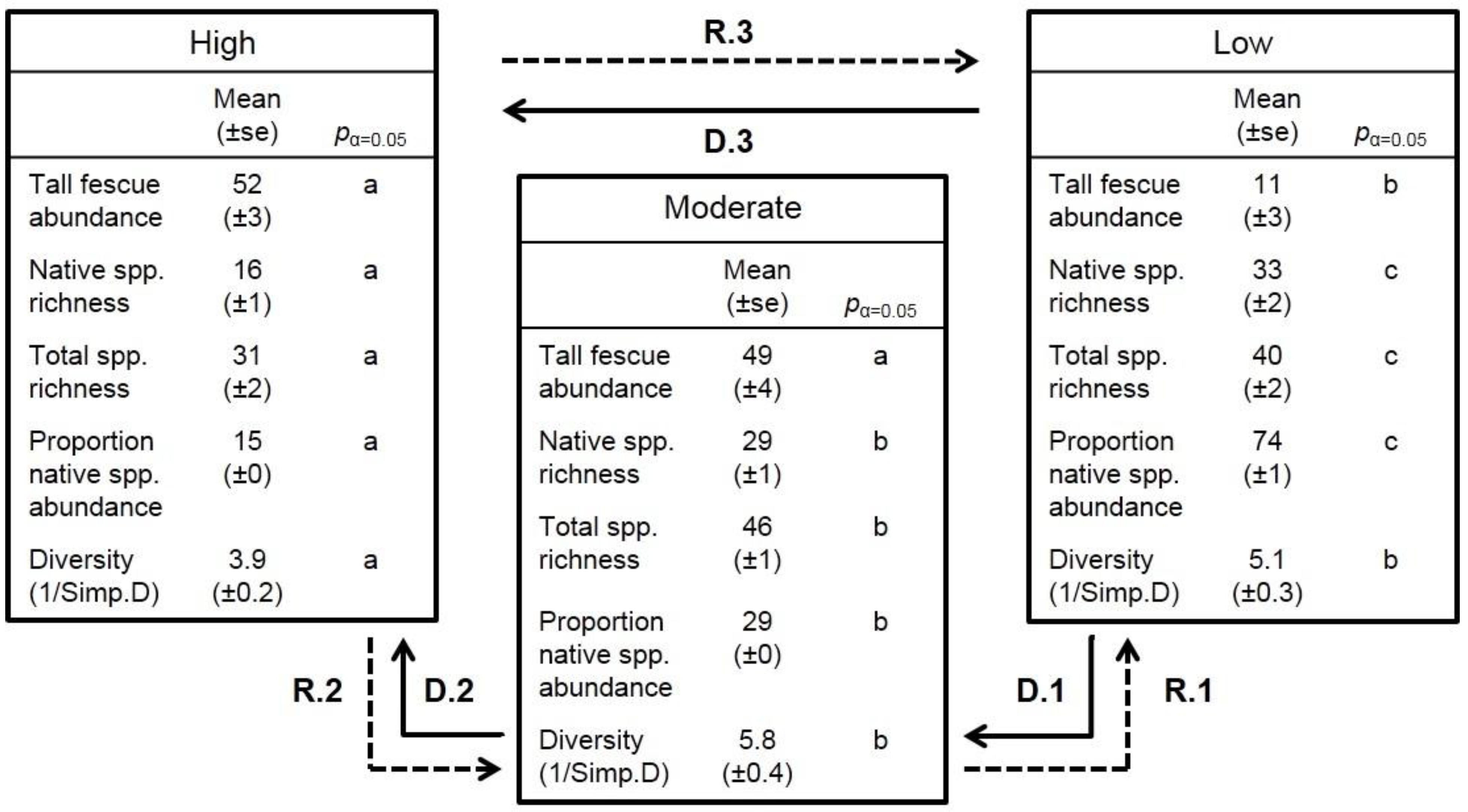
3.3. Degradation States

Three states of vegetation degradation differed in plant community composition in the analysis of dissimilarity (p = 0.03), and showed no overlap when superimposed over the original NMDS ordination (Figure 4). Because of the strong relationships between native species richness and tall fescue abundance in the pattern of degradation, we categorize the three states (hereafter, degradation states) as low, moderate, and high degradation (Table 1). Although each biotic factor varied significantly across the degradation states, soil organic carbon did not vary with degradation (Figure 5). There were also several instances of outliers (Figure 5).

The linear mixed-effect model returned by stepwise AIC model selection included the following variables: tall fescue abundance (t = 2.01, p = 0.05), native species richness (t = 2.06, p < 0.05), and Simpson’s diversity (t = 2.87, p < 0.01). Neither proportion native species abundance, total species richness, nor soil organic carbon was included in the most parsimonious model. However, each varied significantly across the three vegetation states, along with native species richness (Figure 5). Tall fescue abundance did not differ between the high and moderate states, but tall fescue abundance in the low degradation state was significantly lower than the other two states (Figure 5). Conversely, diversity (1/Simpson’s D) was similar between the moderate and low states of degradation, but was significantly lower in the high degradation state (Figure 5).

Figure 4. Ordination of plant species composition from 54 modified Whittaker plots (plots) by Nonmetric Multi-Dimensional Scaling (NMDS) of Canberra distances (k = 4, stress ≈ 12%). Plant communities plotted by floristic degradation state. Grey convex hulls connect tracts and correspond to same labels as in Figure 1. Groups significantly different in adonis test for dissimilarity (p = 0.03).

Figure 4. Ordination of plant species composition from 54 modified Whittaker plots (plots) by Nonmetric Multi-Dimensional Scaling (NMDS) of Canberra distances (k = 4, stress ≈ 12%). Plant communities plotted by floristic degradation state. Grey convex hulls connect tracts and correspond to same labels as in Figure 1. Groups significantly different in adonis test for dissimilarity (p = 0.03).

Figure 5. Box plots of six factors associated with degradation plotted by vegetation degradation states. Overlap among states and outliers suggest individual modified Whittaker plots in transition between states. Boxes include the first and third quartiles; horizontal lines denote data median and open triangles denote data mean. Whiskers extend to one interquartile and outliers are denoted as open circles. Letters indicate statistical difference (p ≤ 0.05) between means in pairwise t-tests.

Figure 5. Box plots of six factors associated with degradation plotted by vegetation degradation states. Overlap among states and outliers suggest individual modified Whittaker plots in transition between states. Boxes include the first and third quartiles; horizontal lines denote data median and open triangles denote data mean. Whiskers extend to one interquartile and outliers are denoted as open circles. Letters indicate statistical difference (p ≤ 0.05) between means in pairwise t-tests.

4. Discussion

As predicted, patterns of plant species richness and abundance clearly segment into three degradation states (Figure 4), which correspond with patterns of two primary degradation factors in these grasslands—tall fescue abundance and a history of severe grazing (Figure 1). While SOC varied substantially across sampled plots (Figure 2B) (Table 2), there was no association between SOC and floristic degradation states (Figure 5). Tall fescue abundance, total and native species richness, proportion native species abundance, and plant species diversity all varied across degradation states (Figure 5).

We use a state-and-transition model (Figure 6) to describe hypothetical degradation and restoration pathways among three states of vegetation degradation in the Grand River Grasslands. Potential pathways, when validated by research or practice, target restoration action and inform restoration goals for management of degraded grassland based on the baseline floristic conditions our results describe.

4.1. Degradation Pattern and Pathways

Our multivariate approach effectively described patterns of vegetation degradation and categorized abundance data from 196 plant species into three distinct vegetation states. As with other applications in which multivariate analyses were used to assess rangeland condition (e.g., [22]), we identified a single species—tall fescue—that described a gradient of vegetation degradation. However, tall fescue abundance alone was not the sole factor that distinguishes degradation states: vegetation degradation was characterized by inverse relationships between richness and abundance of native and exotic species along the gradient of tall fescue invasion (Figure 6). The importance of multiple variables in describing degradation state likely explains variation around the mean values of degradation factors when plotted individually (see whiskers and outliers in Figure 5). These plant communities might also be in transition between states, and further research will determine whether they are following degradation or restoration pathways (Figure 6).

Figure 6. Summary of plant community data for three vegetation degradation states identified by hierarchical cluster analysis of 196 plant species abundance sampled from nine tracts in the Grand River Grasslands of south-central Iowa and north-central Missouri, USA. States (boxes) describe distinct plant communities with similar compositional attributes, and letters give results of pair-wise t-tests (p_{α = 0.05}) comparing each attribute across degradation states; different letters indicate significance at p < 0.05. Characteristic species for each state are given in Table 1. States are linked by hypothetical degradation (D) and restoration (R) pathways to create a simple state-and-transition model [32]. See Discussion for full description of transition pathways.

Figure 6. Summary of plant community data for three vegetation degradation states identified by hierarchical cluster analysis of 196 plant species abundance sampled from nine tracts in the Grand River Grasslands of south-central Iowa and north-central Missouri, USA. States (boxes) describe distinct plant communities with similar compositional attributes, and letters give results of pair-wise t-tests (p_{α = 0.05}) comparing each attribute across degradation states; different letters indicate significance at p < 0.05. Characteristic species for each state are given in Table 1. States are linked by hypothetical degradation (D) and restoration (R) pathways to create a simple state-and-transition model [32]. See Discussion for full description of transition pathways.

These results support a pattern in which native species richness has a stronger negative association with tall fescue abundance than with grazing history, and other exotic species increase with tall fescue abundance [38]. In fact, species abundance data emphasize the pattern shown by species richness: Tall fescue abundance had a stronger negative correlation with proportional abundance of native plants than with native species richness (Figure 1).

A history of severe grazing was associated with the pattern of plant community composition (Figure 1). Generally, light to moderate herbivory maintains native plant species richness in grassland [53,54]. While severe grazing can degrade plant communities [55], native species richness in the Grand River Grasslands did not decline under severe grazing [38]. It appears that grazing history has a greater effect on species abundance than species presence, and grazing might be associated with variation in community composition within vegetation states (Figure 4).

It is clear that grazing affects the pattern of plant community composition but might not have the long-lasting legacy as tall fescue invasion. Severe grazing might be a potential contributor to degradation between the low and moderate degradation states (D.1), but likely has less of a direct influence on other degradation pathways (D.2 and D.3) (Figure 6). Of unknown relevance is the fact that grazing history is documented here at the tract level, and plant community composition at the modified Whittaker plot level (within tracts).

4.2. Managing Pathways between States for Restoration

The literature lacks clear insight into restoration pathways for grassland impacted by both severe grazing and tall fescue invasion, so we offer several hypotheses for restoration to states less degraded by tall fescue. Where heavy grazing is the primary degradation factor, restoration might consist initially of allowing severely grazed tracts to recover from the biotic legacy of overgrazing [9], although highly-degraded vegetation might not respond to grazing cessation alone [56]. Response time of native vegetation to reduced grazing can vary between several years to several decades depending on level of degradation and ecosystem productivity [57,58,59]. In the Grand River Grasslands, native species abundance might increase following grazing cessation [37], but we hypothesize that relative response to grazing cessation decreases as the severity of degradation increases (pathways R.1, R.2, and R.3, respectively) (Figure 6). Invasive plant species—tall fescue, specifically—are the primary factor of degradation in the Grand River Grasslands. Prescribed fire is often used to control invasive plant species [60], but fire alone might be limited to R.1 and maintaining the low degradation state (Figure 6) if native plant abundance is too low to outcompete exotics following fire. For example, prescribed fire alone is ineffective against tall fescue when it occurs in high abundance [27].

Combining ecological disturbances might be more effective than singular management practices. Patch burn-grazing (heterogeneity-based management), in which grazing activity is concentrated within spatially-discrete burned patches, is an effective combination of disturbances with other difficult-to-control invasive plants [61], and with time, might contribute to restoration pathways R.2 and R.3. However, directly restoring highly-degraded grassland to prairie (R.3) within a narrow time frame likely depends upon herbicide treatment [62] and/or reseeding native plants and then managing with fire and grazing [63].

Ultimately, grazing management probably mediates the success of restoring ecosystem processes to restore plant communities (e.g., restoration pathways R.1 and R.2). Heterogeneity-based rangeland management can be stymied by low fuel load and patchy fuel distributions that often occur in overgrazed grassland [64,65]. Tall fescue, specifically, can further complicate patch burn-grazing management by disrupting fire spread, an effect that is exacerbated by fuelbed conditions that follow severe grazing [29,30].

A final consideration is the pattern of soil degradation, and the effect of soil on vegetation restoration response. Many state-and-transition models also consider the soil base [32] because plant-soil interactions can be important in describing degradation [66]. For example, tillage of prairie reduces soil organic carbon and recovery can take several years or decades [67]; thus historical cultivation of these grasslands likely affects degradation and restoration. However, cultivation history remains unknown (Figure 3), and our soil organic carbon data is inconclusive with respect to the pattern of floristic degradation. We suggest further research into soil condition and plant-soil interactions in these and similar grasslands, both to infer cultivation history and inform management.

4.3. Biodiversity Conservation in Working Grassland Landscapes

In North America, the conservation value of human-impacted ecosystems might be under-rated by the assumption that long-term conservation value is contingent on the reversal of temporary degradation factors [68], such as the extirpation of exotic species from grassland. However, undisturbed vegetation states within high quality natural grasslands are not the only plant communities that contribute to grassland conservation. In Europe, scientists and managers distinguish semi-natural grassland as a unique land-use and highlight its role in biodiversity conservation, particularly in agricultural areas [69,70,71]. Semi-natural grasslands reflect the adaptation of wild flora and fauna to centuries of relatively low-intensity land use that created ecosystems distinct from natural communities [69,72,73]. Even when semi-natural areas provide only sub-optimal habitat, they connect otherwise isolated patches of high-quality habitat across the landscape matrix [74].

The old-field plant communities described here resemble European semi-natural grassland in composition, function, and possibly conservation value. For example, the suite of exotic plants in the Grand River Grasslands includes several species and many functionally-similar congenerics found in European semi-natural grasslands [75,76,77]. In the Grand River Grasslands, avian and invertebrate communities within and among tracts overlap considerably [18,20,78] and some species respond to ecological management despite degradation by invasive plants and severe grazing [65]. These patterns suggest that each grassland state contributes to biodiversity conservation at the landscape level, which is consistent with countryside biogeography theory [74]. We encourage further research to develop the concept of semi-natural grassland as a functional term in the mosaic of North American working landscapes.

Whether in Europe or North America, semi-natural grasslands merit attention to their potential conservation value before—and perhaps even without—costly restoration inputs. Plant communities comprised of exotic and native species might constitute novel ecosystems without natural analogy that none-the-less can contribute to the conservation of biodiversity and the restoration of ecosystem services [79]. In degraded North American rangeland, managers should focus on restoration of pattern and process, such as a mosaic of spatially-variable and temporally-variable disturbance regimes and essential habitat structure [80,81].

5. Conclusions

Restoring degraded rangeland is not always straightforward. Multivariate analysis is effective in reducing multi-dimensional data—such as species-level plant community datasets—into categorical groups useful to determine the extent of floristic degradation and inform management decisions when degradation results from multiple causative factors. We show how free-to-download, open-source software can help managers make sense of multi-species data to identify patterns of floristic degradation and predict restoration action. Step-by-step guides to these methods, written by plant ecologists, are available [47,82].

Managers of human-impacted rangeland should recognize its potential conservation value before—and perhaps even without—costly restoration inputs. Plant communities comprised of exotic and native species might constitute novel ecosystems without natural analogy that none-the-less contribute to biodiversity conservation and provision of ecosystem services [79]. In degraded North American rangeland, managers should focus on the restoration of pattern and process, such as a mosaic of spatially-variable and temporally-variable disturbance regimes and essential habitat structure [80,81].

References

1. Ellis, E.C.; Ramankutty, N. Putting people in the map: Anthropogenic biomes of the world. Front. Ecol. Environ. 2008, 6, 439–447. [Google Scholar] [CrossRef]
2. Foley, J.A.; Defries, R.; Asner, G.P.; Barford, C.; Bonan, G.; Carpenter, S.R.; Chapin, F.S.; Coe, M.T.; Daily, G.C.; Gibbs, H.K.; et al. Global consequences of land use. Science 2005, 309, 570–574. [Google Scholar] [CrossRef]
3. Reidsma, P.; Tekelenburg, T.; Vandenberg, M.; Alkemade, R. Impacts of land-use change on biodiversity: An assessment of agricultural biodiversity in the European Union. Agr. Ecosyst. Environ. 2006, 114, 86–102. [Google Scholar] [CrossRef]
4. Flynn, D.F.B.; Gogol-Prokurat, M.; Nogeire, T.; Molinari, N.; Richers, B.T.; Lin, B.B.; Simpson, N.; Mayfield, M.M.; DeClerck, F. Loss of functional diversity under land use intensification across multiple taxa. Ecol. Lett. 2009, 12, 22–33. [Google Scholar] [CrossRef]
5. Fischer, J.; Lindenmayer, D.B.; Manning, A.D. Biodiversity, ecosystem function, and resilience: Ten guiding principles for commodity production landscapes. Front. Ecol. Environ. 2006, 4, 80–86. [Google Scholar] [CrossRef]
6. Scherr, S.J.; McNeely, J.A. Biodiversity conservation and agricultural sustainability: Towards a new paradigm of “ecoagriculture” landscapes. Philos. Trans. R. Soc. Lond. B. Biol. Sci. 2008, 363, 477–494. [Google Scholar] [CrossRef]
7. Jordan, N.; Warner, K.D. Enhancing the multifunctionality of US agriculture. BioScience 2010, 60, 60–66. [Google Scholar] [CrossRef]
8. Scheffer, M.; Carpenter, S.; Foley, J.; Folke, C.; Walker, B. Catastrophic shifts in ecosystems. Nature 2001, 413, 591–596. [Google Scholar] [CrossRef]
9. Whisenant, S.G. Repairing Damaged Wildlands: A Process-Oriented, Landscape-Scale Approach; Cambridge University Press: Cambridge, UK, 1999. [Google Scholar]
10. Sluis, W.J. Patterns of species richness and composition in re-created grassland. Restor. Ecol. 2002, 10, 677–684. [Google Scholar] [CrossRef]
11. Polley, H.W.; Derner, J.D.; Wilsey, B.J. Patterns of plant species diversity in remnant and restored tallgrass prairies. Restor. Ecol. 2005, 13, 480–487. [Google Scholar] [CrossRef]
12. Suding, K.N.; Gross, K.L.; Houseman, G.R. Alternative states and positive feedbacks in restoration ecology. Trends Ecol. Evol. 2004, 19, 46–53. [Google Scholar] [CrossRef]
13. Bestelmeyer, B.T.; Tugel, A.J.; Peacock, G.L.; Robinett, D.G.; Shaver, P.L.; Brown, J.R.; Herrick, J.E.; Sanchez, H.; Havstad, K.M. State-and-transition models for heterogeneous landscapes: A strategy for development and application. Rangel. Ecol. Manag. 2009, 62, 1–15. [Google Scholar] [CrossRef]
14. Boyd, C.S.; Svejcar, T.J. Managing complex problems in rangeland ecosystems. Rangel. Ecol. Manag. 2009, 62, 491–499. [Google Scholar] [CrossRef]
15. Cramer, V.A.; Hobbs, R.J.; Standish, R.J. What’s new about old fields? Land abandonment and ecosystem assembly. Trends Ecol. Evol. 2008, 23, 104–112. [Google Scholar] [CrossRef]
16. Cousins, S.A.O. Landscape history and soil properties affect grassland decline and plant species richness in rural landscapes. Biol. Conserv. 2009, 142, 2752–2758. [Google Scholar] [CrossRef]
17. Briske, D.D.; Fuhlendorf, S.D.; Smeins, F.E. State-and-transition models, thresholds, and rangeland health: A synthesis of ecological concepts and perspectives. Rangel. Ecol. Manag. 2005, 58, 1–10. [Google Scholar] [CrossRef]
18. Debinski, D.M.; Moranz, R.A.; Delaney, J.T.; Miller, J.R.; Engle, D.M.; Winkler, L.B.; McGranahan, D.A.; Barney, R.J.; Trager, J.C.; Stephenson, A.L.; et al. A cross-taxonomic comparison of insect responses to grassland management and land-use legacies. Ecosphere 2011, 2, art131. [Google Scholar] [CrossRef]
19. Hovick, T.J.; Miller, J.R.; Dinsmore, S.J.; Engle, D.M.; Debinski, D.M.; Fuhlendorf, S.D. Effects of fire and grazing on grasshopper sparrow nest survival. J. Wildl. Manag. 2012, 76, 19–27. [Google Scholar] [CrossRef]
20. Moranz, R.A.; Debinski, D.M.; McGranahan, D.A.; Engle, D.M.; Miller, J.R. Untangling the effects of fire, grazing, and land-use legacies on grassland butterfly communities. Biodivers. Conserv. 2012, 21, 2719–2746. [Google Scholar] [CrossRef]
21. Friedel, M.H. Range condition assessment and the concept of thresholds: A viewpoint. J. Range Manag. 1991, 44, 422–426. [Google Scholar] [CrossRef]
22. Van der Westhuizen, H.; Snyman, H.; Fouché, H. A degradation gradient for the assessment of rangeland condition of a semi-arid sourveld in southern Africa. Afr. J. Range Forage Sci. 2005, 22, 47–58. [Google Scholar] [CrossRef]
23. Sadler, R.J.; Hazelton, M.; Boer, M.M.; Grierson, P.F. Deriving state-and-transition models from an image series of grassland pattern dynamics. Ecol. Model. 2010, 221, 433–444. [Google Scholar] [CrossRef]
24. Papini, R.; Valboa, G.; Favilli, F.; L’Abate, G. Influence of land use on organic carbon pool and chemical properties of Vertic Cambisols in central and southern Italy. Agr. Ecosyst. Environ. 2011, 140, 68–79. [Google Scholar] [CrossRef]
25. Bacon, C.W. Toxic endophyte-infected tall fescue and range grasses: Historic perspectives. J. Anim. Sci. 1995, 73, 861–870. [Google Scholar]
26. Clay, K.; Holah, J. Fungal endophyte symbiosis and plant diversity in successional fields. Science 1999, 285, 1742–1744. [Google Scholar] [CrossRef]
27. Madison, L.A.; Barnes, T.G.; Sole, J.D. Effectiveness of fire, disking, and herbicide to renovate tall fescue fields to Northern Bobwhite habitat. Wildl. Soc. Bull. 2001, 29, 706–712. [Google Scholar]
28. Rudgers, J.A.; Koslow, J.M.; Clay, K. Endophytic fungi alter relationships between diversity and ecosystem properties. Ecol. Lett. 2004, 7, 42–51. [Google Scholar] [CrossRef]
29. McGranahan, D.A.; Engle, D.M.; Fuhlendorf, S.D.; Miller, J.R.; Debinski, D.M. An invasive cool-season grass complicates prescribed fire management in a native warm-season grassland. Nat. Areas J. 2012, 32, 208–214. [Google Scholar] [CrossRef]
30. McGranahan, D.A.; Engle, D.M.; Miller, J.R.; Debinski, D.M. An invasive grass increases live fuel proportion and reduces fire spread in a simulated grassland. Ecosystems 2013, 16, 158–169. [Google Scholar] [CrossRef]
31. Westoby, M.; Walker, B.; Noy-Meir, I. Opportunistic management for rangelands not at equilibrium. J. Range Manag. 1989, 42, 266–274. [Google Scholar] [CrossRef]
32. Stringham, T.K.; Krueger, W.C.; Shaver, P.L. State and transition approach modeling: An ecological process. J. Range Manag. 2003, 56, 106–113. [Google Scholar] [CrossRef]
33. IEM “Climodat” Reports; IEM Iowa Environmental Mesonet, Iowa State University Department of Agronomy: Lamoni, IA, USA. Available online: http://mesonet.agron.iastate.edu/climodat/index.phtml?station=IA4585&report=17 (accessed on 31 May 2011).
34. USDA-SCS, Soil Survey of Ringgold County, Iowa; United States Department of Agriculture: Washington, DC, USA, 1992.
35. USDA-NRCS. Web Soil Survey Data for Ringgold County, Iowa; Natural Resource Conservation Service, United States Department of Agriculture. Available online: http://websoilsurvey.nrcs.usda.gov (accessed on 25 February 2011).
36. Miller, J.R.; Morton, L.W.; Engle, D.M.; Debinski, D.M.; Harr, R.N. Nature reserves as catalysts for landscape change. Front. Ecol. Environ. 2012, 10, 144–152. [Google Scholar] [CrossRef]
37. Rosburg, T.R.; Glenn-Lewin, D.C. Effects of Fire and Atrazine on Pasture and Remnant Prairie Plant Species in Southern Iowa. In Proceedings of the Twelfth North American Prairie Conference, Cedar Falls, IA, USA, 5–9 August 1990; pp. 107–112.
38. McGranahan, D.A.; Engle, D.M.; Wilsey, B.J.; Fuhlendorf, S.D.; Miller, J.R.; Debinski, D.M. Grazing and an invasive grass confound spatial pattern of exotic and native grassland plant species richness. Basic Appl. Ecol. 2012, 13, 654–662. [Google Scholar] [CrossRef]
39. Stohlgren, T.J.; Bull, A.; Otsuki, Y. Comparison of rangeland vegetation sampling techniques in the Central Grasslands. J. Range Manag. 1998, 51, 164–172. [Google Scholar] [CrossRef]
40. Daubenmire, R. A canopy-coverage method of vegetational analysis. Northwest Sci. 1959, 33, 43–64. [Google Scholar]
41. Mann, L.K. Changes in soil carbon storage after cultivation. Soil Sci. 1986, 142, 279–288. [Google Scholar] [CrossRef]
42. Fuhlendorf, S.D.; Zhang, H.; Tunnell, T.R.; Engle, D.M.; Cross, A.F. Effects of grazing on restoration of southern mixed prairie soils. Restor. Ecol. 2002, 10, 401–407. [Google Scholar] [CrossRef]
43. He, N.P.; Zhang, Y.H.; Yu, Q.; Chen, Q.S.; Pan, Q.M.; Zhang, G.M.; Han, X.G. Grazing intensity impacts soil carbon and nitrogen storage of continental steppe. Ecosphere 2011, 2, art8. [Google Scholar] [CrossRef]
44. United States Department of Agriculture-National Cooperative Soil Survey (USDA-NCSS). National Cooperative Soil Characterization Data. Available online: http://ssldata.nrcs.usda.gov/default.htm (accessed on 25 February 2011).
45. Altesor, A.; Pineiro, G.; Lezama, F.; Jackson, R.B.; Sarasola, M.; Paruelo, J.M. Ecosystem changes associated with grazing in subhumid South American grasslands. J. Veg. Sci. 2006, 17, 323–332. [Google Scholar] [CrossRef]
46. Legendre, P.; Legendre, L. Numerical Ecology; Elsevier: Amsterdam, The Netherlands, 1998. [Google Scholar]
47. Dixon, P. VEGAN, a package of R functions for community ecology. J. Veg. Sci. 2003, 14, 927–930. [Google Scholar] [CrossRef]
48. Oksanen, J.; Blanchet, F.G.; Kindt, R.; Legendre, P.; O’Hara, R.G.; Simpson, G.L.; Solymos, P.; Stevens, M.H.H.; Wagner, H. Vegan: Community Ecology Package. Available online: http://cran.r-project.org/package=vegan (accessed on 25 January 2011).
49. R Development Core Team, R: A Language and Environment for Statistical Computing. R Foundation for Statistical Computing: Vienna, Austria, 2011.
50. Beals, M.L. Understanding community structure: A data-driven multivariate approach. Oecologia 2006, 150, 484–495. [Google Scholar] [CrossRef]
51. Pinheiro, J.; Bates, D.; DebRoy, S.; Sarkar, D.; R Core Team. nlme: Linear and Nonlinear Mixed Effects Models. Available online: http://cran.r-project.org/web/packages/nlme/index.html (accessed on 22 May 2011).
52. Burnham, K.P.; Anderson, D.R. Model Selection and Multimodel Inference: A Practical Information-Theoretic Approach; Springer: New York, NY, USA, 2002. [Google Scholar]
53. Milchunas, D.G.; Sala, O.E.; Lauenroth, W.K. A generalized model of the effects of grazing by large herbivores on grassland community structure. Am. Nat. 1988, 132, 87–106. [Google Scholar]
54. Burns, C.E.; Collins, S.L.; Smith, M.D. Plant community response to loss of large herbivores: Comparing consequences in a South African and a North American grassland. Biodivers. Conserv. 2009, 18, 2327–2342. [Google Scholar] [CrossRef]
55. Pieper, R.D. Ecological Implications of Livestock Grazing. In Ecological Implications of Livestock Herbivory in the West; Vavra, M., Laycock, W.A., Pieper, R.D., Eds.; USA Society for Range Management: Denver, CO, USA, 1994; pp. 177–211. [Google Scholar]
56. Laycock, W.A. Stable states and thresholds of range condition on North American rangelands: A viewpoint. J. Range Manag. 1991, 44, 427–433. [Google Scholar] [CrossRef]
57. Gardner, J.L. Effects of thirty years of protection from grazing in desert grassland. Ecology 1950, 31, 44–50. [Google Scholar] [CrossRef]
58. Fleischner, T.L. Ecological costs of livestock grazing in western North America. Conserv. Biol. 1994, 8, 629–644. [Google Scholar]
59. Harrison, Y.; Shackleton, C. Resilience of South African communal grazing lands after the removal of high grazing pressure. Land Degrad. Dev. 1999, 10, 225–239. [Google Scholar] [CrossRef]
60. DiTomaso, J.M.; Brooks, M.L.; Allen, E.B.; Minnich, R.; Rice, P.M.; Kyser, G.B. Control of invasive weeds with prescribed burning. Weed Technol. 2006, 20, 535–548. [Google Scholar] [CrossRef]
61. Cummings, D.C.; Fuhlendorf, S.D.; Engle, D.M. Is altering grazing selectivity of invasive forage species with patch burning more effective than herbicide treatments? Rangel. Ecol. Manag. 2007, 60, 253–260. [Google Scholar] [CrossRef]
62. Barnes, T.G. Using herbicides to rehabilitate native grasslands. Nat. Areas J. 2007, 27, 56–65. [Google Scholar] [CrossRef]
63. Bouressa, E.L.; Tugel, A.J.; Peacock, G.L.; Jackson, R.D. Burning and grazing to promote persistence of warm-season grasses sown into a cool-season pasture. Ecol. Restor. 2010, 28, 40–45. [Google Scholar] [CrossRef]
64. McGranahan, D.A.; Engle, D.M.; Fuhlendorf, S.D.; Winter, S.J.; Miller, J.R.; Debinski, D.M. Spatial heterogeneity across five rangelands managed with pyric-herbivory. J. Appl. Ecol. 2012, 49, 903–910. [Google Scholar] [CrossRef]
65. McGranahan, D.A.; Engle, D.M.; Fuhlendorf, S.D.; Winter, S.L.; Miller, J.R.; Debinski, D.M. Inconsistent outcomes of heterogeneity-based management underscore importance of matching evaluation to conservation objectives. Environ. Sci. Policy 2013, 31, 53–60. [Google Scholar] [CrossRef]
66. Rietkerk, M.; Van de Koppel, J. Alternate stable states and threshold effects in semi-arid grazing systems. Oikos 1997, 79, 69–76. [Google Scholar] [CrossRef]
67. Baer, S.G.; Kitchen, D.J.; Blair, J.M.; Rice, C.W. Changes in ecosystem structure and function along a chronosequence of restored grasslands. Ecol. Appl. 2002, 12, 1688–1701. [Google Scholar] [CrossRef]
68. Young, T.P. Restoration ecology and conservation biology. Biol. Conserv. 2000, 92, 73–83. [Google Scholar] [CrossRef]
69. Poschlod, P.; Bakker, J.P.; Kahmen, S. Changing land use and its impact on biodiversity. Basic Appl. Ecol. 2005, 6, 93–98. [Google Scholar] [CrossRef]
70. Öckinger, E.; Smith, H.G. Landscape composition and habitat area affects butterfly species richness in semi-natural grasslands. Oecologia 2006, 149, 526–534. [Google Scholar] [CrossRef]
71. Lindborg, R.; Bengtsson, J.; Berg, Å.; Cousins, S.A.O.; Eriksson, O.; Gustafsson, T.; Hasund, K.P.; Lenoir, L.; Pihlgren, A.; Sjödin, E.; et al. A landscape perspective on conservation of semi-natural grasslands. Agr. Ecosyst. Environ. 2008, 125, 213–222. [Google Scholar] [CrossRef]
72. Efetha, Å.A.; Eriksson, O.; Berglund, H. Species abundance patterns of plants in Swedish semi-natural pastures. Ecography 2006, 18, 310–317. [Google Scholar]
73. Kleijn, D.; Baquero, R.A.; Clough, Y.; Díaz, M.; Esteban, J.; Fernández, F.; Gabriel, D.; Herzog, F.; Holzschuh, A.; Jöhl, R.; et al. Mixed biodiversity benefits of agri-environment schemes in five European countries. Ecol. Lett. 2006, 9, 243–254. [Google Scholar] [CrossRef]
74. Ricketts, T.H.; Daily, G.C.; Ehrlich, P.R.; Fay, J.P. Countryside biogeography of moths in a fragmented landscape: Biodiversity in native and agricultural habitat. Conserv. Biol. 2001, 15, 378–388. [Google Scholar] [CrossRef]
75. Lindborg, R.; Eriksson, O. Effects of restoration on plant species richness and composition in scandinavian semi-natural grasslands. Restor. Ecol. 2004, 12, 318–326. [Google Scholar] [CrossRef]
76. Pykälä, J. Plant species responses to cattle grazing in mesic semi-natural grassland. Agr. Ecosyst. Environ. 2005, 108, 109–117. [Google Scholar] [CrossRef]
77. Pykälä, J. Effects of restoration with cattle grazing on plant species composition and richness of semi-natural grasslands. Biodivers. Conserv. 2003, 12, 2211–2226. [Google Scholar] [CrossRef]
78. Pillsbury, F.C.; Miller, J.R.; Debinski, D.M.; Engle, D.M. Another tool in the toolbox? Using fire and grazing to promote bird diversity in highly fragmented landscapes. Ecosphere 2011, 2, art28. [Google Scholar] [CrossRef]
79. Seastedt, T.R.; Hobbs, R.J.; Suding, K.N. Management of novel ecosystems: Are novel approaches required? Front. Ecol. Environ. 2008, 6, 547–553. [Google Scholar] [CrossRef]
80. Tews, J.; Brose, U.; Grimm, V.; Tielbörger, K.; Wichmann, M.C.; Schwager, M.; Jeltsch, F. Animal species diversity driven by habitat heterogeneity/diversity: The importance of keystone structures. J. Biogeogr. 2004, 31, 79–92. [Google Scholar] [CrossRef]
81. Fuhlendorf, S.D.; Engle, D.M.; Elmore, R.D.; Limb, R.F.; Bidwell, T.G. Conservation of pattern and process: Developing an alternative paradigm of rangeland management. Rangel. Ecol. Manag. 2012, 65, 579–589. [Google Scholar] [CrossRef]
82. Oksanen, J. Multivariate Analysis of Ecological Communities in R: Vegan Tutorial. Available online: http://cc.oulu.fi/~jarioksa/opetus/metodi/vegantutor.pdf (accessed on 12 March 2013).
Appendix
Table A1. Attributes for 54 modified Whittaker plot plant communities used in hierarchical clustering (Figure A1) based on 196 plant species abundance sampled from nine tracts in the Grand River Grasslands of south-central Iowa and north-central Missouri, USA. Plot code represents nomenclature used in Figure A1: “Pasture.Patch.Plot” uses an abbreviation of the pasture name and the first letter of cardinal directions to locate each plot nested within patches [20]. Pasture names correspond with NMDS ordination in Figure 1A of the main text. Native species richness, total species richness, Proportion native abundance, and Simpson’s diversity (1/D) are summarized in Figure 5 in the main text.
Plot CodeTractGrazing HistoryFloristic Degradation StateNative Species RichnessTotal Species RichnessProportion Native AbundanceSimpson’s Diversity (1/D)
Gil.C.NGillelandSeverely grazedHigh14310.33.04
Gil.C.SGillelandSeverely grazedHigh18390.143.88
Gil.N.NGillelandSeverely grazedHigh18380.062.4
Gil.N.SGillelandSeverely grazedHigh15310.035.92
Gil.S.NGillelandSeverely grazedHigh8280.013.23
Gil.S.SGillelandSeverely grazedHigh28510.384.06
LT. C.SLee TrailUngrazedMedium28340.806.02
LT.C.NLee TrailUngrazedMedium35460.477.67
LT.E.NLee TrailUngrazedHigh13200.282.81
LT.E.SLee TrailUngrazedHigh16260.052.77
LT.W.NLee TrailUngrazedMedium26320.853.58
LT.W.SLee TrailUngrazedMedium26320.453.23
Paw.E.NPawneeUngrazedMedium41520.975.5
Paw.E.SPawneeUngrazedMedium39450.945.28
Paw.S.NPawneeUngrazedMedium49530.994.22
Paw.S.SPawneeUngrazedMedium46530.835.74
Paw.W.NPawneeUngrazedMedium31390.904.98
Paw.W.SPawneeUngrazedMedium40510.982.93
PyN.N.NPyland NorthSeverely grazedHigh12290.023.44
PyN.N.SPyland NorthSeverely grazedHigh26430.314.8
PyN.S.NPyland NorthSeverely grazedLow21390.229.69
PyN.S.SPyland NorthSeverely grazedLow36540.284.52
PyN.W.NPyland NorthSeverely grazedLow28470.127.18
PyN.W.SPyland NorthSeverely grazedLow26460.376.35
PyS.N.NPyland SouthSeverely grazedLow35490.414.98
PyS.N.SPyland SouthSeverely grazedLow33530.457.99
PyS.S.NPyland SouthSeverely grazedLow33500.315.88
PyS.S.SPyland SouthSeverely grazedLow29480.134.62
PyS.W.NPyland SouthSeverely grazedLow32480.527.06
PyS.W.SPyland SouthSeverely grazedLow25420.223.71
PyW.C.NPyland WestSeverely grazedLow23370.144.48
PyW.C.SPyland WestSeverely grazedMedium30470.293.42
PyW.N.NPyland WestSeverely grazedMedium27470.25.61
PyW.N.SPyland WestSeverely grazedMedium31480.163.92
PyW.S.NPyland WestSeverely grazedMedium24390.336.8
PyW.S.SPyland WestSeverely grazedMedium30470.524.96
Rch.N.NRichardsonUngrazedHigh9180.072.81
Rch.N.SRichardsonUngrazedHigh21320.072.02
Rch.S.NRichardsonUngrazedHigh13270.12.81
Rch.S.SRichardsonUngrazedHigh21330.153.35
Rch.W.NRichardsonUngrazedHigh13200.113.21
Rch.W.SRichardsonUngrazedHigh17300.33.7
RN.E.NRinggold NorthUngrazedLow33360.996.31
RN.E.SRinggold NorthUngrazedLow222314.71
RN.S.NRinggold NorthUngrazedLow29300.983.94
RN.S.SRinggold NorthUngrazedLow27280.993.81
RN.W.NRinggold NorthUngrazedLow35390.999.42
RN.W.SRinggold NorthUngrazedLow394317.27
RS.C.NRinggold SouthUngrazedLow31430.557.24
RS.C.SRinggold SouthUngrazedLow45520.678.85
RS.N.NRinggold SouthUngrazedLow21310.394.16
RS.N.SRinggold SouthUngrazedLow30420.354.87
RS.S.NRinggold SouthUngrazedLow30360.384.94
RS.S.SRinggold SouthUngrazedLow33420.285.27
Figure A1. Results of hierarchical clustering using the Canberra distance matrix to identify three vegetation states based on plant community composition (see Experimental section in main text). Codes represent each of 54 modified Whittaker plots used for vegetation sampling (see Table A1 for explanation of nomenclature and description of plant community attributes). The two High degradation groups are combined into a single vegetation state based on similarity of plant community attributes listed in Table A1 (see Experimental section in main text).
Land 02 00328 g007