Design and Interpretation of Intensity Analysis Illustrated by Land Change in Central Kalimantan, Indonesia

Abstract

Intensity Analysis has become popular as a top-down hierarchical accounting framework to analyze differences among categories, such as changes in land categories over time. Some aspects of interpretation are straightforward, while other aspects require deeper thought. This article explains how to interpret Intensity Analysis with respect to four concepts. First, we illustrate how to analyze whether error could account for non-uniform changes. Second, we explore two types of the large dormant category phenomenon. Third, we show how results can be sensitive to the selection of the domain. Fourth, we explain how Intensity Analysis’ symmetric top-down hierarchy influences interpretation with respect to temporal processes, for which changes during a time interval influence the sizes of the categories at the final time, but not at the initial time. We illustrate these concepts by applying Intensity Analysis to changes during one time interval (2000–2004) in a part of Central Kalimantan for the land categories Forest, Bare and Grass.

1. Introduction

Intensity Analysis is a quantitative framework to account for differences among categories as summarized by a square transition matrix for which the rows’ categories are identical to the columns’ categories [1]. Analysis of land change through time is the most common application of the framework. Intensity Analysis’ seminal article [2] has more than 200 citations, including one in the first issue of the journal Land [3]. Applications of Intensity Analysis to land change span six continents, including: Africa [4], Asia [5], Australia [6], Europe [7], North America [1], and South America [8]. Through many case studies, we have identified four recurring important concepts that users must understand in order to apply and to interpret Intensity Analysis properly. The purpose of this article is to describe those concepts and to offer guidance concerning how to address the concepts in a manner that applies generally to other case studies.

Our article examines concepts that apply to a single time interval, while the concepts apply also to case studies that analyze each of several consecutive time intervals. The first concept addresses how to interpret results when researchers suspect that the data have error but do not know exactly how much error. The second concept concerns the large dormant category phenomenon, where the inclusion of a single large category influences the results for all other categories. The third concept relates to the fact that it is frequently not obvious how to select the domain for a case study, so we illustrate conceptually how Intensity Analysis can be sensitive to the selection of the domain, with particular attention to inclusion of various amounts of persistence. The fourth concept relates to the fact that Intensity Analysis uses a top-down hierarchy in which the sizes of the categories at the initial and final times help to set uniform baselines for comparison to the observed transitions. However, the amounts of change and persistence during a time interval influence the sizes of the categories at the final time, but do not influence the sizes of the categories at the initial time. Thus, it can be more intuitive to interpret change intensities that are conditional on the sizes of the categories at the initial time, rather than the final time, depending on whether one views the change processes as top-down or bottom-up.

This article illustrates the concepts with a case study that has three land categories, because three categories show the concepts as clearly as possible. Our case study is on the island of Borneo in Central Kalimantan, Indonesia. Figure 1 shows the location of the study area and its land changes between 2000 and 2004 among the categories: Forest, Bare and Grass. The domain covers 1,896 square kilometers between the Sebangau and Katingan Rivers in the Sebangau National Park. The natural vegetation is mainly tropical peatland swamp forest, which has experienced extensive deforestation and forest degradation [9]. Commercial logging started during the 1960s in the Central Kalimantan province of Indonesian Borneo, and one-fifth of Kalimantan’s forests had been logged by 1980 [10]. Land management practices have impaired the natural functioning of the peatland ecosystem and have increased the ecosystem’s susceptibility to fire [11]. Forest losses occurred during the drought of the 1982–1983 El Niño when 2.7 million ha of tropical rainforest burned, and again during the 1997–1998 El Niño when almost five million hectares of forests were damaged [12]. Peatland fires occurred again in Central Kalimantan during the 2002 El Niño [13,14]. Deforestation in this region can lead to serious global consequences because tropical peat swamp forest ecosystems host exceptionally high biodiversity and immense amounts of carbon [14,15]. Therefore, it is important to study land change in Central Kalimantan.

Figure 1. Map in the upper left shows the location of the study site in the southern part of the island of Borneo, which is shared by Indonesia, Malaysia and Burnei. Kalimantan is the Indonesian portion of Borneo. The study site is in Central Kalimantan Province. The middle and lower maps on the left show land-cover categories at 2000 and 2004. Maps on the right show changes during 2000–2004.

Figure 1. Map in the upper left shows the location of the study site in the southern part of the island of Borneo, which is shared by Indonesia, Malaysia and Burnei. Kalimantan is the Indonesian portion of Borneo. The study site is in Central Kalimantan Province. The middle and lower maps on the left show land-cover categories at 2000 and 2004. Maps on the right show changes during 2000–2004.

2. Methods

2.1. Data

The underlying data are two Landsat scenes from path 118 and row 62: one ETM+ scene from 16 July 2000 and one TM scene from 17 June 2004. The satellite images were geometrically corrected with ground control points that were evenly distributed in space, and the root mean square error was within one pixel. Atmospheric correction was performed using the FLAASH module, available in the ENVI 4.0 software. The atmospheric correction removed the influence of aerosols that affect reflectance values primarily in the short wavelength regions of the electromagnetic spectrum.

We applied unsupervised image classification using the ISODATA clustering algorithm with 100 initial spectral clusters. The spectral clusters were labeled using the information from color composites, NDVI images, land-cover spectral reflectance characteristics, and field knowledge. Three land-cover categories were assigned: Forest, Bare, and Grass. Forest is peat swamp forest. Bare is bare soil including burn scars that do not have vegetation. Grass is fern grass, sparse shrubs, and regenerating secondary forest. Then we applied a majority filter with a window size of 3 by 3 pixels to reduce isolated pixels in the land-cover maps. A mask eliminated pixels that are water or clouds at either time point. We do not have information concerning the accuracy of the maps because we do not have ground information for 2000 and 2004.

After we created the classified maps, we constructed a transition matrix by overlaying the two land-cover maps. Table 1 shows the matrix in terms of percent of the domain. The nine entries in the upper left show the transitions. The three diagonal entries indicate persistence of categories, and the six off-diagonal entries indicate change from one category to a different category. We appended a column on the right that shows the categorical totals at 2000 and a row at the bottom that shows the categorical totals at 2004. We also appended an additional column on the right that indicates loss by category, and an additional row at the bottom that indicates gain by category. The entry in the extreme lower right indicates total change as a percent of the domain.

Table 1. Transitions as a percent of the domain. Superscript α indicates a systematically avoiding transition. Superscript τ indicates a systematically targeting transition.

		2004			2000	Interval
		Forest	Bare	Grass	Total	Loss
2000	Forest	76.8	5.7α	4.0	86.5	9.7
	Bare	4.0α	5.5	1.8τ	11.2	5.7
	Grass	1.1	0.3τ	0.9	2.4	1.5
2004	Total	81.9	11.4	6.7	100.0
Interval	Gain	5.1	6.0	5.8		16.9

Table 1. Transitions as a percent of the domain. Superscript α indicates a systematically avoiding transition. Superscript τ indicates a systematically targeting transition.

		2004			2000	Interval
		Forest	Bare	Grass	Total	Loss
2000	Forest	76.8	5.7α	4.0	86.5	9.7
	Bare	4.0α	5.5	1.8τ	11.2	5.7
	Grass	1.1	0.3τ	0.9	2.4	1.5
2004	Total	81.9	11.4	6.7	100.0
Interval	Gain	5.1	6.0	5.8		16.9

2.2. Change Budget

Table 2 gives the mathematical notation that our article uses. Equation (1) gives the total change by summing all entries in the matrix then subtracting the diagonal entries, which show persistence. Equation (1) expresses the total change as a percent of the domain by multiplying by 100% and dividing by the number of pixels in the domain. Total change can be separated into two parts: quantity change and allocation change. Equation (2) gives the quantity change expressed as a percent of the domain. The inner summation over i in the numerator of Equation (2) computes the net change for category j by adding the transitions in which category j gains, i.e., C_ij, and then subtracting the transitions in which category j loses, i.e., C_ji. The MAXIMUM function selects the categories for which the net change is positive, and then the summation over j accumulates the positive net changes. When one category gains, another category loses, and so the total net gain of all the categories is equal to the total net loss of the categories. Equation (3) computes the allocation disagreement in a manner that shows how quantity change and allocation change sum to the total change.

Table 2. Mathematical notation for Intensity Analysis.

Symbol	Meaning
J	number of categories, which equals 3 in our case study
i	index for a category at the interval’s initial time point
j	index for a category at the interval’s final time point
m	index for the losing category for the selected transition
n	index for the gaining category for the selected transition
Cij	number of pixels that transition from category i to category j
S	total change as percent of domain, which equals the uniform intensity for the category level
Gj	intensity of gain of category j relative to size of category j at final time
Li	intensity of loss of category i relative to size of category i at initial time
Rin	intensity of transition from category i to category n relative to size of category i at initial time where i≠n
Wn	uniform intensity of transition from all non-n categories to category n relative to size of all non-n categories at initial time
Qmj	intensity of transition from category m to category j relative to size of category j at final time where j≠m
Vm	uniform intensity of transition from all non-m categories to category j relative to size of all non-m categories at final time
EGj	hypothesized commission of category j error at final time
OGj	hypothesized omission of category j error at final time
ELi	hypothesized commission of category i error at initial time
OLi	hypothesized omission of category i error at initial time

Table 2. Mathematical notation for Intensity Analysis.

Symbol	Meaning
J	number of categories, which equals 3 in our case study
i	index for a category at the interval’s initial time point
j	index for a category at the interval’s final time point
m	index for the losing category for the selected transition
n	index for the gaining category for the selected transition
Cij	number of pixels that transition from category i to category j
S	total change as percent of domain, which equals the uniform intensity for the category level
Gj	intensity of gain of category j relative to size of category j at final time
Li	intensity of loss of category i relative to size of category i at initial time
Rin	intensity of transition from category i to category n relative to size of category i at initial time where i≠n
Wn	uniform intensity of transition from all non-n categories to category n relative to size of all non-n categories at initial time
Qmj	intensity of transition from category m to category j relative to size of category j at final time where j≠m
Vm	uniform intensity of transition from all non-m categories to category j relative to size of all non-m categories at final time
EGj	hypothesized commission of category j error at final time
OGj	hypothesized omission of category j error at final time
ELi	hypothesized commission of category i error at initial time
OLi	hypothesized omission of category i error at initial time

(1)

(2)

(3)

2.3. Intensity Analysis

Intensity Analysis is a mathematical framework that compares a uniform intensity to observed intensities of temporal changes among categories. We use Intensity Analysis at two levels: category and transition.

At the category level, we compare S from Equation (1) to G_j and L_i from Equations (4) and (5). Equation (4) gives the observed intensity with which category j gains, relative to the size of category j at the final time point. If each category were to gain with the same intensity, then all the intensities would equal S from Equation (1). In other words, if the total change were to occur uniformly in the domain, then the intensity of each categorical gain would equal the global intensity S. If G_j > S, then we say category j is an active gainer. If G_j < S, then we say category j is a dormant gainer. This concept concerning gains applies also to losses. Equation 5 gives the observed intensity with which category i loses, relative to the size of category i at the initial time point. If each category were to lose with the same intensity, then all the intensities would equal S. If L_i > S, then we say category i is an active loser. If L_i < S, then we say category i is a dormant loser.

(4)

(5)

Equations (6) and (7) concern Intensity Analysis for the transition from an arbitrary category i to a particular gaining category n. Equation (6) gives the observed intensity with which category n gains from category i. If category n were to gain with the same intensity from all not i categories, then R_in would equal W_n from Equation (7). If R_in > W_n, then we say that the gain of n targets i. If R_in < W_n, then we say that the gain of n avoids i.

(6)

(7)

Equations (8) and (9) concern Intensity Analysis for the transition from a particular losing category m to a different category j. Equation (8) gives the observed intensity with which category m loses to another category j. If category m were to lose with the same intensity from all not j categories, then Q_mj would equal V_m from Equation (9). If Q_mj > V_m, then we say that j targets the loss of m. If Q_mj < V_m, then we say that j avoids the loss of m. If the denominators of the ratios in Equations (4–6, and 8) are zero, then the change in the numerators must be zero, and the ratio does not exist.

(8)

(9)

The transition from category m to category n is a systematically targeting transition when the gain of n targets m while n targets the loss of m, i.e., when R_mn > W_n while Q_mn > V_m. The transition from category m to category n is a systematically avoiding transition when the gain of n avoids m while n avoids the loss of m, i.e., when R_mn < W_n while Q_mn < V_m.

2.4. Error Analysis

We do not have reference information to measure errors in the maps from the two time points. Nevertheless, we suspect our maps have some errors and we wonder whether errors in the maps could account for the deviations from uniform intensities that Intensity Analysis reveals. Equations in this subsection allow us to compute the minimum hypothetical error in the data that could account for the deviation between the uniform change intensity S and the intensity of each categorical gain or loss [16]. We compute these hypothetical errors based on a null hypothesis that the intensity of change is uniform. A larger hypothetical error gives stronger evidence against this null hypothesis.

Equations (10–13) compute the hypothetical error in the map of the final time that could account for a deviation between G_j and S. Equations (10,11) apply to categories where G_j > S, which are Bare and Grass for the case study. Equation (10) computes the number of pixels of observed gain of category j that we hypothesize are errors of commission of category j at the final time. The Intensity Analysis web site [17] gives a mathematical derivation for Equation (10) and other equations that follow a similar logic, i.e., Equations (12,14,16). Equation (11) computes the commission error intensity of category j at the final time, where the numerator of Equation (11) is the hypothesized commission error of category j and the denominator is the size of observed gain of category j. Equations (12,13) apply to categories where G_j < S, which is Forest for the case study. Equation (12) computes the number of pixels of observed gain of a non-Forest category that we hypothesize are errors of omission of Forest at the final time. Equation (13) computes the omission error intensity, which is the result from Equation (11) divided by the size of the hypothesized gain of Forest. Commission error intensity is 100% minus User’s accuracy. Omission error intensity is 100% minus Producer’s accuracy.

(10)

(11)

(12)

(13)

Equations (14–17) compute the hypothetical error in the map of the initial time that could account for a deviation between L_i and S. Equations (14,15) apply to categories where L_i > S, which are Bare and Grass for the case study. Equation (14) computes the number of pixels of observed loss of category i that we hypothesize are errors of commission of category i at the initial time. Equation (15) computes the commission error intensity of category i at the initial time, where the numerator of Equation (15) is the hypothesized commission error of category i and the denominator is the size of observed loss of category i. Equations (16) and (17) apply to categories where L_i < S, which is Forest for the case study. Equation (16) computes the number of pixels of observed loss of a non-Forest category that we hypothesize are errors of omission of Forest at the initial time. Equation (17) computes the omission error intensity, which is the result from Equation (16) divided by the size of the hypothesized gain of Forest.

(14)

(15)

(16)

(17)

3. Results

3.1. Change Budget

Figure 2 shows the total change as the percent of the domain separated into components of quantity and allocation. Change occurs in 16.9 percent of the domain, and 12.3 of those percentage points derive from allocation change. Figure 3 shows the gain, persistence and loss of each category. The size of a category at 2000 is the union of its persistence and loss. The size of a category at 2004 is the union of its persistence and gain. Forest accounts for 86 percent of the domain at 2000 and 81 percent at 2004.

Figure 2. Total change separated into quantity and allocation.

Figure 2. Total change separated into quantity and allocation.

Figure 3. Gain, persistence and loss by category.

Figure 3. Gain, persistence and loss by category.

3.2. Intensity Analysis

Figure 4 shows the intensity of gains and losses by category. If a bar stops before the uniform line, then the category is dormant; thus, Forest is a dormant loser and a dormant gainer. If a bar extends beyond the uniform line, then the category is active; thus, both Grass and Bare are active losers and active gainers.

Figure 4. Intensity of gains and losses by category.

Figure 4. Intensity of gains and losses by category.

Figure 5, Figure 6, Figure 7 compare the observed transition intensities to the hypothesized uniform transition intensities. If a bar stops before the uniform line, then the transition avoids. If a bar extends beyond the uniform line, then the transition targets. The upper part of Figure 5 shows that the gain of Forest targets Grass and avoids Bare, while the lower part of Figure 5 shows that Grass targets and Bare avoids the loss of Forest. Figure 6 shows that the gain of Bare targets Grass and avoids Forest, while Grass targets and Forest avoids the loss of Bare. Figure 7 shows that the gain of Grass targets Bare and avoids Forest, while Bare targets and Forest avoids the loss of Grass. Thus, the systematically targeting transitions are from Grass to Bare and from Bare to Grass; while the systematically avoiding transitions are from Bare to Forest and from Forest to Bare.

Figure 5. Intensity of transitions given Forest’s gain on the positive axis and given Forest’s loss on the negative axis.

Figure 5. Intensity of transitions given Forest’s gain on the positive axis and given Forest’s loss on the negative axis.

Figure 6. Intensity of transitions given Bare’s gain on the positive axis and given Bare’s loss on the negative axis.

Figure 6. Intensity of transitions given Bare’s gain on the positive axis and given Bare’s loss on the negative axis.

Figure 7. Intensity of transitions given Grass’ gain on the positive axis and given Grass’ loss on the negative axis.

Figure 7. Intensity of transitions given Grass’ gain on the positive axis and given Grass’ loss on the negative axis.

3.3. Error Analysis

Figure 8 shows the intensities of the hypothetical errors that could account for the deviations between observed category level change intensities and the hypothesized uniform change intensity, i.e., the deviations in Figure 4. The three bars in Figure 8 concerning the map of 2004 indicate hypothetical errors that could account for deviations from a uniform gain. Specifically, if the actual omission error intensity for Forest at 2004 is less than 67 percent, then there is evidence that Forest is dormant in terms of gains. The three bars concerning the map of 2000 indicate hypothetical errors that could account for deviations from a uniform loss. Specifically, if the actual omission error intensity for Forest at 2000 is less than 38 percent, then there is evidence that Forest is dormant in terms of losses. By similar logic, if the commission error intensities are less than 81 percent for both Bare and Grass at both 2000 and 2004, then there is evidence that Bare and Grass are active in terms of both gains and losses, because 81 percent is the minimum among the bars for Bare and Grass in Figure 8.

Figure 8. Hypothetical error intensities within the change region that could account for deviations from uniform category level losses and gains. If the actual error intensities are less than the ones in the figure, then there is evidence that the category level gains and losses are non-uniform.

Figure 8. Hypothetical error intensities within the change region that could account for deviations from uniform category level losses and gains. If the actual error intensities are less than the ones in the figure, then there is evidence that the category level gains and losses are non-uniform.

4. Discussion

4.1. Error Analysis

It is common that researchers do not know the sizes and types of errors in the data, especially because satellite images are widely available for historic dates but it is impossible to go back in time to collect ground reference information that would be necessary to assess accuracy. If accuracy information were to exist, then it would be desirable to compare the hypothetical error intensities to the actual error intensities, but ignorance of actual errors is not a sufficient reason to ignore possible errors and is not a sufficient reason to disregard historic satellite images. Researchers can draw on their experience with similar types of classifications as researchers interpret the hypothetical errors. Figure 8 shows that the Forest omission hypothetical error is substantially smaller than the other hypothetical errors, thus the conclusion that Forest is dormant in terms of losses has weaker evidence than the other conclusions concerning categorical losses and gains shown in Figure 4.

4.2. Large Dormant Category Phenomenon

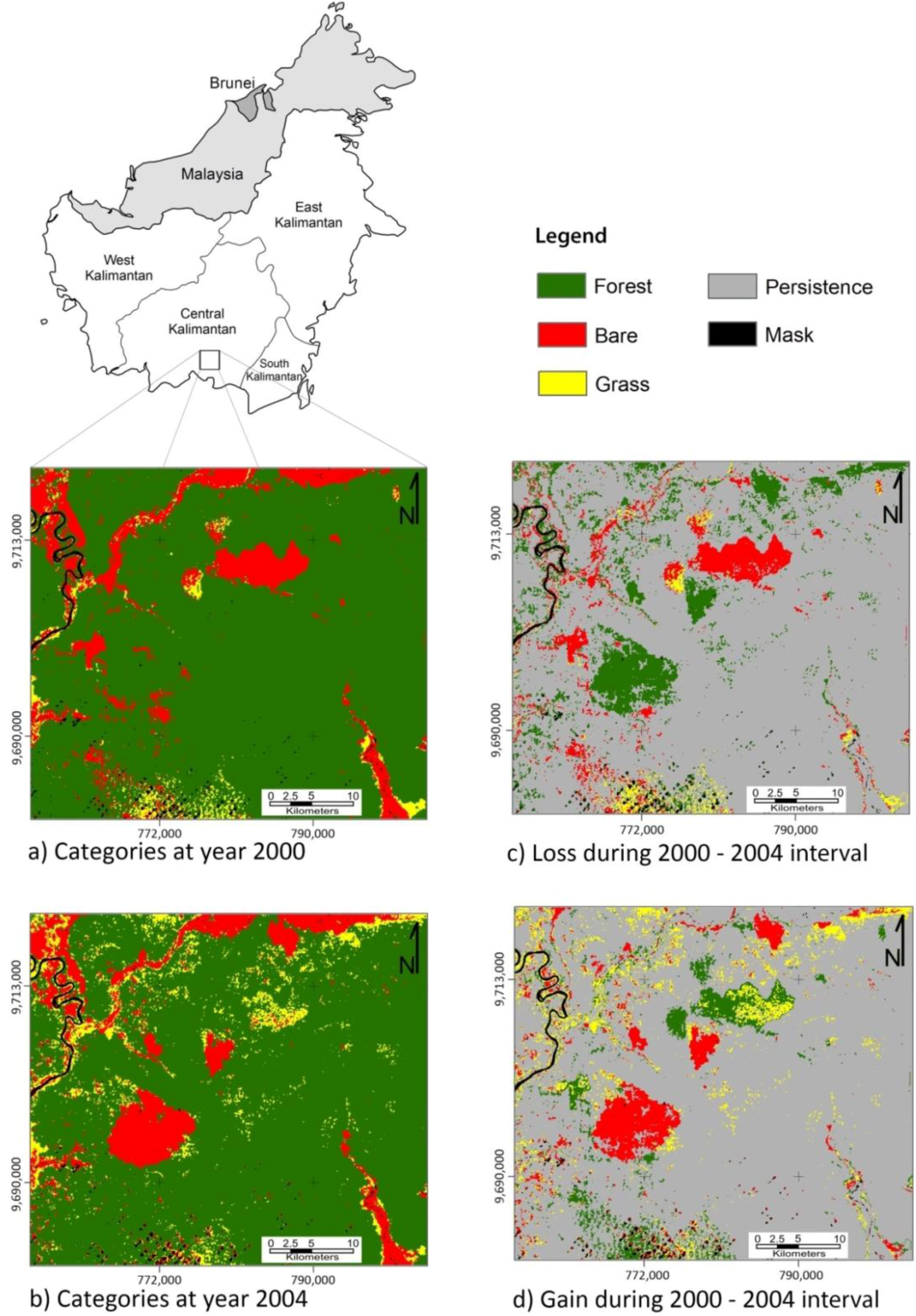
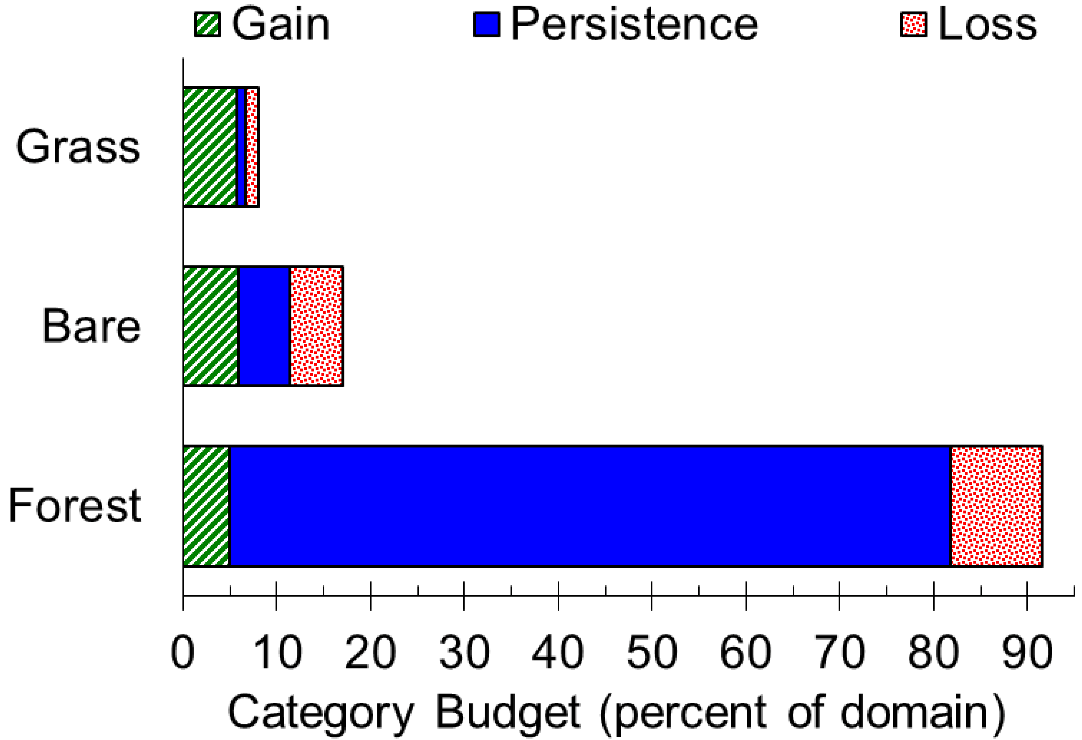
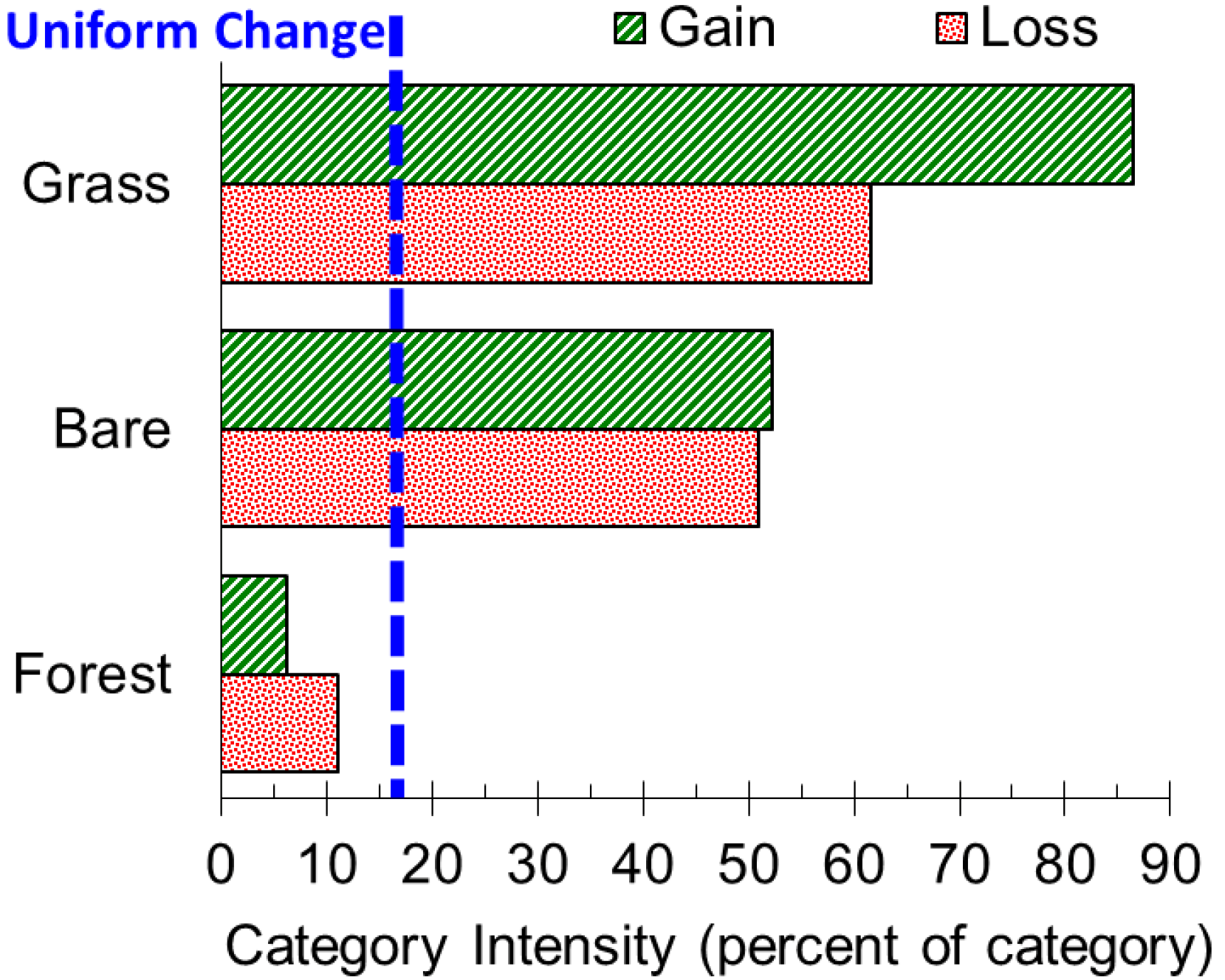
The Kalimantan case study illustrates one type of the large dormant category phenomenon, in which the presence of a large dormant category causes the intensities of other categories to be greater than they would be in the absence of the large dormant category [1]. Forest accounts for the majority of the domain at both time points (Table 1), and Forest is dormant in terms of both gains and losses (Figure 4), thus Forest is a large dormant category. 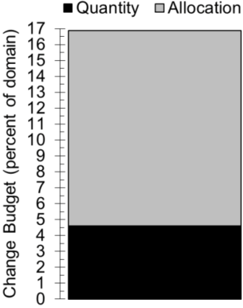Forest’s large size plays a role in the results that Forest is dormant in both gains and losses, and that gains of both Bare and Grass avoid Forest, while Forest avoids the losses of both Bare and Grass (Figure 6, Figure 7). Nevertheless, Forest plays a substantial role in the total change, because change occurs in approximately 17 percent of the Central Kalimantan domain, and 15 of those percentage points involve transitions with Forest (Table 1). Forest is dormant due mainly to its large persistence, which is included in the denominators of Equations (4,5). We performed sensitivity analysis to see how much Forest persistence must be eliminated from the domain in order for Forest to become active. We found that if 89 percent or more of the Forest persistence were eliminated from the domain, then Forest would become active in losses, and Forest would become a targeting category in the four transitions analyzed in Figure 6, Figure 7. If 97 percent or more of the Forest persistence were eliminated from the domain, then Forest would become active also in gains.

Our case study illustrates one type of the large dormant category phenomenon that is different than a second type in which the large dormant category plays a small role in total change. Water is a typical example of the second type of large dormant category. Water might be necessary to include in some land change studies where humans convert water to land via infill or convert land to water via dams. It is not clear how much of the persistent water should be included in a study of change, especially for coastal studies where most of the water category persists as ocean. The size of any category affects the intensities of other categories; thus, researchers can be tempted to exclude water to eliminate this effect. In fact, we masked water from the Kalimantan case study because water is small and not particularly relevant to our research question. If water were excluded from an analysis, then the analysis might miss some important transitions that involve water, depending on the research question. The large dormant category phenomenon requires more research to determine general principles concerning how to select a study’s domain.

4.3. Sensitivity to the Selection of the Domain

Selection of the domain is influential regardless of whether one uses Intensity Analysis or some other analytical technique. For example, Equation 1 computes the total change as a domain’s percent, which includes persistence in the denominator. Equation (1) is usually the first calculation in an investigation of land change. This subsection illustrates how Intensity Analysis is sensitive to the amount of persistence that the domain includes for each category, thus it is usually helpful to consider how the results of Intensity Analysis can be sensitive to the selection of the domain, especially concerning possible elimination of some persistence or entire categories, such as water.

Table 3, Table 4, Table 5, Table 6 give four examples to illustrate the major points. Each table has ten pixels, six of which show change, thus S = 6/10. All tables are identical in terms of the changes, meaning the off-diagonal transitions are identical across the four tables. Each table is symmetric, meaning each table is identical to its transpose. The only differences among the tables are the amounts of persistence for each category, which are on the matrices’ diagonal entries.

Table 3 shows that the size of Bare equals the size of Grass at both time points. Intensity Analysis computes transition intensities, given the sizes of the categories at the time points. The transition from Bare to Forest is larger than the transition from Grass to Forest, thus Intensity Analysis indicates that the gain of Forest targets Bare and avoids Grass. The transition from Forest to Bare is larger than the transition from Forest to Grass, thus Intensity Analysis indicates that Bare targets the loss of Forest and Grass avoids the loss of Forest. For Table 3, Table 4, Table 5, 3/4 of the final Forest derives from Forest’s gain and 3/4 of the initial Forest loses. Thus, Forest is active in both gains and losses for Table 3, Table 4, Table 5, because 3/4 is greater than 6/10.

Table 4 shows that the size of Bare is twice the size of Grass at both time points. The transition from Bare to Forest is twice the transition from Grass to Forest, and the transition from Forest to Bare is twice the transition from Forest to Grass. Thus, Intensity Analysis indicates the intensities are uniform for both transitions from Forest and for both transitions to Forest.

Table 5 shows that the size of Bare is five times the size of Grass at both time points. The transition from Bare to Forest is less than five times the transition from Grass to Forest, thus the gain of Forest avoids Bare and targets Grass. The transition from Forest to Bare is less than five times the transition from Forest to Grass, thus Bare avoids the loss of Forest and Grass targets the loss of Forest.

Table 6 shows that the size of Bare is twice the size of Grass at both time points. The transition from Bare to Forest is twice the transition from Grass to Forest, and the transition from Forest to Bare is twice the transition from Forest to Grass. Thus, Intensity Analysis indicates that the intensities are uniform for both transitions from Forest and for both transitions to Forest, as in Table 4. In contrast to Table 4, Table 6 indicates that 3/7 of the final Forest derives from gain and 3/7 of the initial Forest loses. Thus, Forest is dormant in both gains and losses, because 3/7 is less than 6/10.

Table 3. Matrix that shows Forest’s gain targets Bare and Bare targets Forest’s loss.

		Final Time			Initial	Interval
		Forest	Bare	Grass	Total	Loss
Initial Time	Forest	1	2	1	4	3
	Bare	2	1	0	3	2
	Grass	1	0	2	3	1
Final	Total	4	3	3	10
Interval	Gain	3	2	1		6

Table 3. Matrix that shows Forest’s gain targets Bare and Bare targets Forest’s loss.

		Final Time			Initial	Interval
		Forest	Bare	Grass	Total	Loss
Initial Time	Forest	1	2	1	4	3
	Bare	2	1	0	3	2
	Grass	1	0	2	3	1
Final	Total	4	3	3	10
Interval	Gain	3	2	1		6

Table 4. Matrix that shows uniform transition intensities to Forest and from Forest for active Forest.

		Final Time			Initial	Interval
		Forest	Bare	Grass	Total	Loss
Initial Time	Forest	1	2	1	4	3
	Bare	2	2	0	4	2
	Grass	1	0	1	2	1
Final	Total	4	4	2	10
Interval	Gain	3	2	1		6

Table 4. Matrix that shows uniform transition intensities to Forest and from Forest for active Forest.

		Final Time			Initial	Interval
		Forest	Bare	Grass	Total	Loss
Initial Time	Forest	1	2	1	4	3
	Bare	2	2	0	4	2
	Grass	1	0	1	2	1
Final	Total	4	4	2	10
Interval	Gain	3	2	1		6

Table 5. Matrix that shows Forest’s gain avoids Bare and Bare avoids Forest’s loss.

		Final Time			Initial	Interval
		Forest	Bare	Grass	Total	Loss
Initial Time	Forest	1	2	1	4	3
	Bare	2	3	0	5	2
	Grass	1	0	0	1	1
Final	Total	4	5	1	10
Interval	Gain	3	2	1		6

Table 5. Matrix that shows Forest’s gain avoids Bare and Bare avoids Forest’s loss.

		Final Time			Initial	Interval
		Forest	Bare	Grass	Total	Loss
Initial Time	Forest	1	2	1	4	3
	Bare	2	3	0	5	2
	Grass	1	0	0	1	1
Final	Total	4	5	1	10
Interval	Gain	3	2	1		6

Table 6. Matrix that shows uniform transition intensities to Forest and from Forest for dormant Forest.

		Final Time			Initial	Interval
		Forest	Bare	Grass	Total	Loss
Initial Time	Forest	4	2	1	7	3
	Bare	2	0	0	2	2
	Grass	1	0	0	1	1
Final	Total	7	2	1	10
Interval	Gain	3	2	1		6

Table 6. Matrix that shows uniform transition intensities to Forest and from Forest for dormant Forest.

		Final Time			Initial	Interval
		Forest	Bare	Grass	Total	Loss
Initial Time	Forest	4	2	1	7	3
	Bare	2	0	0	2	2
	Grass	1	0	0	1	1
Final	Total	7	2	1	10
Interval	Gain	3	2	1		6

We had considered excluding persistence from the equations as we developed Intensity Analysis. Specifically, we considered making the denominator of Equation (6) equal to the loss of category i rather than the size of i at the initial time, in which case we would have made the denominator of Equation (7) equal to the sum of losses of all not n categories rather than the size of all not n categories at the initial time. Also, we considered making the denominator of Equation (8) equal to the gain of category j rather than the size of j at the final time, in which case we would have made the denominator of Equation (9) equal to the sum of gains of all not m categories rather than the size of all not m categories at the final time. Alas, we realized that this would defeat the purpose of Intensity Analysis, because it would imply that all the Forest transitions in Table 3, Table 4, Table 5, Table 6 have uniform intensities equal to one, but Table 3, Table 4, Table 5, Table 6 have different patterns that we designed purposely to portray different processes. The next subsections describe how Intensity Analysis can offer insight to the relationship between pattern and process.

4.4. Top-Down Hierarchy and Temporal Processes

Intensity Analysis has a top-down hierarchy in which broader information determines the context for more detailed information. Specifically, Intensity Analysis interprets category level intensities L_i and G_j relative to the broader intensity of total change S (Table 2). Then, Intensity Analysis interprets transition level intensities R_in and Q_mj relative to category level intensities W_n and V_m. Categories’ sizes influence the calculation of the detailed transition level intensities, while the various transition intensities do not influence the category level calculations. For example, it is possible to compute Equations (1–5) using knowledge of only the matrix’s diagonal entries and category sizes at the initial and final times. Then, Intensity Analysis computes the transition intensities, conditional on the category sizes.

Furthermore, Intensity Analysis’ equations concerning the matrix’s rows are symmetric with its equations concerning the matrix’s columns. However, a temporal change process is not symmetric in time because the change during a time interval influences the sizes of the categories at the final time but not at the initial time. Therefore, it can be more intuitive to interpret intensities that are conditional on the initial time, than to interpret intensities that are conditional on the final time. Specifically, at the category level, it can be more intuitive to compare L_i to S, than to compare G_j to S, because L_i is conditional on the size of category i at the initial time but G_j is conditional on the size of category j at the final time. For the same reason, it can be more intuitive to compare transition intensities R_in to W_n than to compare Q_mj to V_m at the transition level. For intensities that are conditional on the final time, the degree of difficulty of interpretation depends on how one envisions the hierarchy of the change process. If a change process is top-down, i.e., where broader categorical changes dictate the detailed transitions, then interpretation is straight forward because the change process matches the structure of Intensity Analysis. If change processes are bottom-up, i.e., where various detailed transitions combine to form broader patterns at the category level, then it can be challenging to interpret results that are conditional on the final time. To illustrate, let us revisit Table 3, Table 4, Table 5, Table 6.

We designed symmetry into Table 3, Table 4, Table 5, Table 6 to illustrate the point that Intensity Analysis is symmetric with respect to the initial and final times. Table 3, Table 4, Table 5, Table 6 are symmetric with respect to the diagonal, thus the tables’ symmetry matches the symmetry of the equations in Intensity Analysis. In the hierarchy of Intensity Analysis, the calculation of transition intensities during the interval does not influence the sizes of the categories at the initial time, which makes temporal sense. Also, the calculation of transition intensities during the interval does not influence the sizes of the categories at the final time, which can be initially counter intuitive, but can still make sense when the process has a top-down hierarchy. For example, consider a case where the initial map is completely Forest, and the transition from Forest to Bare is twice the size of the transition from Forest to Grass, as in the Forest row of Table 6. Imagine that a process of growth of construction drives the conversion to Bare, while a process of growth of logging drives the conversion to Grass. Intensity Analysis models the change by accounting first for the fact that the size of Bare is twice the size of Grass at the final time. Therefore, Intensity Analysis would consider both transitions from Forest to be uniform. The explanation would be that the growth of construction is twice the growth of logging in the entire domain, and these two top-down processes explain why the size of the transition from Forest to Bare is twice the size of the transition from Forest to Grass. In this explanation, the two broader category level top-down processes can completely account for the transitions. This illustrates how one must interpret results by considering the change processes.

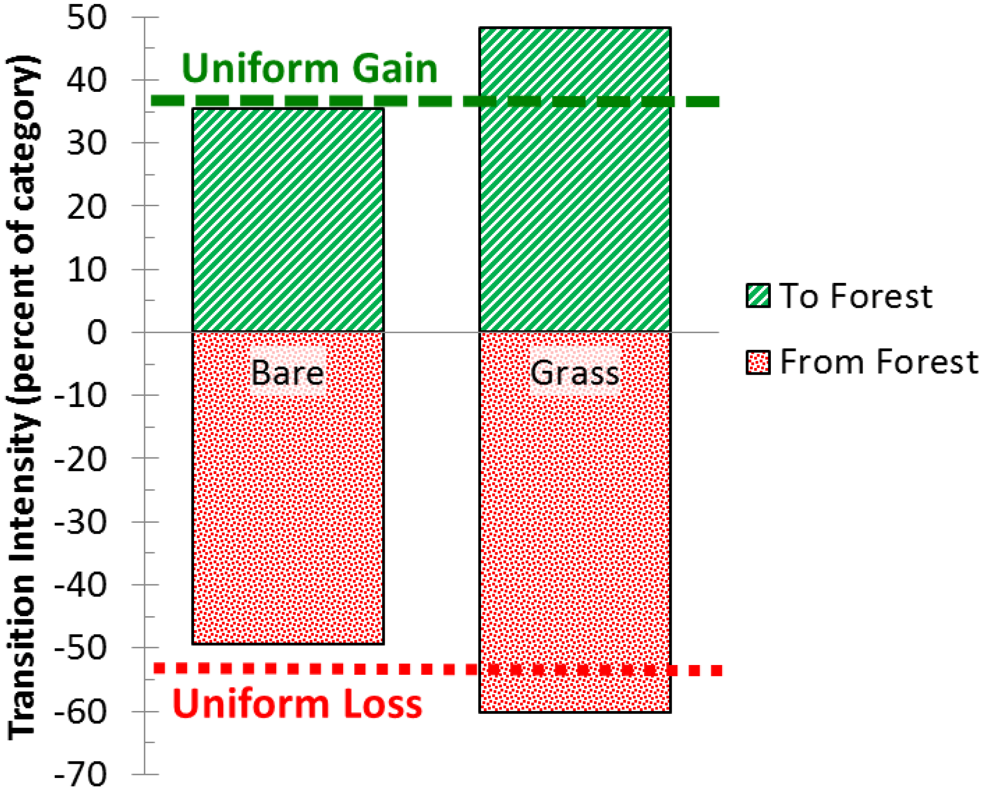
Let us illustrate further with our case study by considering transitions to Forest, while focusing on transition intensities that are conditional on the initial time. We hypothesize that Forest would grow more from Grass than from Bare, because we hypothesize a natural process of recovery from Bare to Grass to Forest. However, the size of the transition from Bare to Forest is larger than the size of the transition from Grass to Forest (Table 1). This seems at first to contradict our hypothesis, but Intensity Analysis resolves the contradiction by considering the sizes of Bare and Grass at the initial time. There is more Bare than Grass at the initial time; thus, if Forest were to gain with uniform intensity from both Bare and Grass at the initial time, then the size of the transition from Bare to Forest would be larger than the size of the transition from Grass to Forest. Intensity Analysis shows that the gain of Forest targets Grass and avoids Bare (Figure 5), which matches our hypothesized process of Forest gain.

Now let us consider the transitions from Forest, while focusing on transition intensities that are conditional on the final time. We hypothesize that the change processes of Forest loss in our study area are fire, agriculture, and logging [15]. Uncontrolled fires are likely to produce Bare, whereas agriculture and logging are likely to produce Grass. The size of the transition from Forest to Bare is larger than the size of the transition from Forest to Grass (Table 1), which seems initially to support a hypothesis that fire is more responsible than other drivers for Forest’s loss. However, transition intensities indicate that Bare avoids the loss of Forest while Grass targets the loss of Forest (Figure 5), which seems to support a hypothesis that fire is less responsible than other drivers for Forest’s loss. The transition intensity from Forest to Bare is less than the transition intensity from Forest to Grass due in part to the fact that Bare is more prevalent than Grass at the final time. However, the sizes at the final time are influenced by persistence and change during the time interval. This example demonstrates how results from Intensity Analysis can help to formulate hypotheses concerning process of change.

If Intensity Analysis were to give information identical to the information that we could see easily by a direct comparison of the sizes of the transitions, then there would be no need for Intensity Analysis. Intensity Analysis probes the transition matrix to reveal the matrix’s detailed patterns. The transition matrix describes patterns of change, which are caused by processes of change. Researchers must use qualitative knowledge concerning processes of change in order to interpret Intensity Analysis in a manner that can help to develop a cause and effect understanding. Intensity Analysis can help to assess the evidence for a particular hypothesized process of change, and can help to develop new hypotheses concerning processes of change. For proper interpretation, researchers must consider whether the hypothesized processes of change match the hierarchical structure of Intensity Analysis.

4.5. Next Steps in Research Agenda

We are beginning to develop a method to detect whether top-down processes can account for detailed transitions or whether various bottom-up transitions are required to account for a particular matrix, because usually there can be many possible combinations of transitions that are consistent with a set of marginal totals and persistence for each category. If the matrix’s marginal totals could explain all the transitions, then there would be evidence that top-down processes are operating. If the matrix’s marginal totals cannot explain the transitions, then there would be evidence that bottom-up processes are operating. Future research should examine this approach to link patterns with processes.

It is interesting to compare Intensity Analysis to the Markov approach, which is a popular method to analyze a transition matrix [1,18,19]. Markov’s architecture assumes bottom-up processes in which the transition intensities within each row of the matrix determine the changes over time. The Markov matrix computes the proportion of the initial category that transitions to categories at the subsequent time, conditional on the size of the selected initial category, and independent of the other initial categories. For the Kalimantan case study, the Markov transition from Forest to Bare is greater than the Markov transition from Forest to Grass, because the size of the transition from Forest to Bare is greater than the size of the transition from Forest to Grass. The Markov matrix ignores the size of the categories at the final time, which explains why Markov’s results are different than Intensity Analysis’ results concerning the transition intensities for a selected losing category. Markov is not designed to analyze a pattern of gains in the way Intensity Analysis does, because Markov does not compare the distribution of transitions within each column.

Some potential applications of Intensity Analysis are not temporal, and would therefore not have the above-mentioned complications concerning interpretation of temporal cause and effect relationships. For example, Intensity Analysis could compare two classifications of a single image, where the rows indicate the categories according to one method of classification and the columns indicate the categories according to an alternative method of classification. The research question would ask how the two classifications are associated. In this situation, there is not a cause and effect relationship among the rows and columns, because the process of one classification does not affect the process of the other classification. For such cases, the symmetrical architecture of Intensity Analysis matches the symmetry of the research question concerning the association between the two methods of classification.

5. Conclusions

This article examines the design of Intensity Analysis and offers guidance concerning its interpretation. We illustrate four important concepts using a matrix of transitions among the categories Forest, Bare, and Grass over one time interval in Central Kalimantan, Indonesia. These four concepts concern: error analysis, the large dormant category phenomenon, sensitivity to the selection of the domain, and the top-down hierarchical symmetric structure of Intensity Analysis. The results illustrate how Intensity Analysis gives information that is different than the information obtained from a direct comparison of the sizes of the entries in the transition matrix. In our case study, Forest is the only dormant category for both gains and losses, in spite of being involved in most of the changes. The transition from Forest to Bare is systematically avoiding, in spite of being the largest transition. These types of insights can help researchers test and develop hypotheses concerning processes of change. This article’s concepts are generally applicable, so we hope researchers of other case studies will benefit from these ideas during the application and interpretation of Intensity Analysis.

References

1. Aldwaik, S.Z.; Pontius, R.G., Jr. Intensity analysis to unify measurements of size and stationarity of land changes by interval, category, and transition. Landsc. Urban. Plan. 2012, 106, 103–114. [Google Scholar] [CrossRef]
2. Pontius, R.G., Jr.; Shusas, E.; McEachern, M. Detecting important categorical land changes while accounting for persistence. Agric. Ecosyst. Environ. 2004, 100, 251–268. [Google Scholar]
3. Gitau, M.; Bailey, N. Multi-Layer assessment of land use and related changes for decision support in a coastal zone watershed. Land 2012, 1, 5–31. [Google Scholar] [CrossRef]
4. Alo, C.A.; Pontius, R.G., Jr. Identifying systematic land-cover transitions using remote sensing and GIS: The fate of forests inside and outside protected areas of Southwestern Ghana. Environ. Plan. B 2008, 35, 280–295. [Google Scholar] [CrossRef]
5. Villamor, G.B.; Pontius, R.G., Jr.; Van Noordwijk, M. Agroforest’s growing role in carbon losses from Jambi (Sumatra), Indonesia. Reg. Environ. Change 2013. submitted. [Google Scholar]
6. Manandhar, R.; Odeh, I.O.A.; Pontius, R.G., Jr. Analysis of twenty years of categorical land transitions in the lower Hunter of New South Wales, Australia. Agric. Ecosyst. Environ. 2010, 135, 336–346. [Google Scholar] [CrossRef]
7. Plata Rocha, W.; Gómez Delgado, M.; Bosque Sendra, J. Cambios de Usos del Suelo y Expansión Urbana en la Comunidad de Madrid (1990–2000). In Scripta. Nova. Revista Electrónica de Geografía y Ciencias Sociales; Universidad de Barcelona: Barcelona, Spain, 2009; Volume XIII, p. 293. [Google Scholar]
8. Romero-Ruiz, M.H.; Flantua, S.G.A.; Tansey, K.; Berrio, J.C. Landscape transitions in savannas of northern South America: Land use/cover changes since 1987 in the Llanos Orientales of Colombia. Appl. Geogr. 2011, 32, 766–776. [Google Scholar]
9. Langner, A.; Miettinen, J.; Siegert, F. Land cover change 2002–2005 in Borneo and the role of fire derived from MODIS imagery. Glob. Change Biol. 2007, 13, 2329–2340. [Google Scholar] [CrossRef]
10. Ramankutty, N.; Graumlich, L.; Achard, F.; Alves, D.; Chhabra, A.; DeFries, R.S.; Foley, J.A.; Geist, H.; Houghton, R.A.; Goldewijk, K.K.; et al. Land-Use and Land-Cover Change: Local Process and Global Impacts; Lambin, E.F., Geist, H.J., Eds.; Springer: Berlin/Heidelberg, Germany, 2006; Chapter 2; pp. 9–39. [Google Scholar]
11. Page, S.E.; Siegert, F.; Rieley, J.O.; Boehm, H.D.V.; Jaya, A.; Limin, S. The amount of carbon released from peat and forest fires in Indonesia during 1997. Nature 2002, 420, 61–65. [Google Scholar] [CrossRef]
12. Barber, C.V.; Schweithelm, J. Trial by Fire-Forest Fire and Forestry Policy in Indonesia’s Era of Crisis and Reform; World Resources Institute: Washington, DC, USA, 2000; pp. 1–76. [Google Scholar]
13. Siegert, F.; Zhukov, B.; Oertel, D.; Limin, S.; Page, S.E.; Rieley, J.O. Peat fires detected by the BIRD satellite. Int. J. Remote Sens. 2004, 25, 3221–3230. [Google Scholar]
14. Hirano, T.; Segah, H.; Kusin, K.; Limin, S.; Takahashi, H.; Osaki, M. Effects of disturbances on the carbon balance of tropical peat swamp forests. Glob. Change Biol. 2012, 18, 3410–3422. [Google Scholar] [CrossRef]
15. Miettinen, J.; Shi, C.G.; Liew, S.C. Deforestation rates in insular Southeast Asia between 2000 and 2010. Glob. Change Biol. 2011, 17, 2261–2270. [Google Scholar] [CrossRef]
16. Aldwaik, S.Z.; Pontius, R.G., Jr. Map errors that could account for deviations from a uniform intensity of land change. Int. J. Geogr. Inf. Sci. 2013. [Google Scholar] [CrossRef]
17. Intensity Analysis. Available online: https://sites.google.com/site/intensityanalysis/ (accessed on 6 June 2013).
18. Takada, T.; Miyamoto, A.; Hasegawa, S. Derivation of a yearly transition probability matrix for land-use dynamics and its applications. Landsc. Ecol. 2010, 25, 561–572. [Google Scholar] [CrossRef]
19. Runfola, D.M.; Pontius, R.G., Jr. Measuring the temporal instability of land change using the Flow matrix. Int. J. Geogr. Inf. Sci. 2013. [Google Scholar] [CrossRef]