Article

Incorporating Topography into Landscape Continuity Analysis—Hong Kong Island as a Case Study

1
Department of Geography, Hebrew University of Jerusalem, Mount Scopus, Jerusalem 91905, Israel
2
Department of Geography, The University of Hong Kong, The Jockey Club Tower, Centennial Campus, Pokfulam Road, Hong Kong, China
*
Author to whom correspondence should be addressed.
Land 2013, 2(4), 550-572; https://doi.org/10.3390/land2040550
Submission received: 25 July 2013 / Revised: 22 September 2013 / Accepted: 9 October 2013 / Published: 16 October 2013
(This article belongs to the Special Issue Landscape Perspectives on Environmental Conservation)

Abstract

:
The increase in population and the expansion of built-up areas into natural and agricultural areas results in more than just loss of open spaces surrounding cities. Reduced accessibility to nature, visual intrusion of buildings into natural viewsheds, and changes in runoff requires us to assess these impacts on open spaces. Our aim in this paper was to examine and demonstrate how topography can be incorporated into modeling and analyzing environmental impacts of cities. Taking Hong Kong Island as a case study, we used historical topographic maps to map changes in the built-up areas between 1930 and 2006. We analyzed changes in three variables representing different kinds of human impacts: landscape continuity, visibility of built-up areas, and runoff from built-up areas. We show that consideration of topography (both natural and artificial) is critical to understand spatial patterns of land use and of human impacts on open spaces. The methods employed here can be applied to examine and visualize the potential effects of future and proposed development plans.

1. Introduction

Expansion of built-up areas due to ongoing growth in the world’s population leads to conflicts between urban development pressures and conservation planning, and presents challenges for planners, landscape ecologists and conservation biologists around the world [1]. We define open areas or open spaces as areas that are not comprised of permanent structures such as roads or buildings. Open areas provide ecosystems services and values [2], and human impacts in these spaces may be reversible and are usually less intensive than in built-up areas. Built-up areas (e.g., cities, roads, villages, or industrial parks) affect their surroundings in various ways, including: air and water pollution [3], noise nuisance [4], the fragmentation and contraction of natural habitats [5], the construction of obstacles for the migration of wildlife [6], climate modification (e.g., urban heat island effect, [7]), an increase in floods and runoff [8], night-time light pollution [9], and finally, visual effects on the way people perceive their surroundings and their chances of having a wilderness experience [10].
Landscape continuity may be envisioned as the degree to which open landscape features are connected between themselves (which is important for animal movement and accessibility), and the degree at which open spaces are free from the impacts of adjacent built-up areas (as in [6,11]). The impact of built-up areas and roads on landscape continuity depends on both structural and functional factors that relate to: (1) built-up area characteristics, e.g., urban, suburban, village or industrial; (2) the surrounding land cover type, e.g., planted or natural forests, orchards or agricultural fields; (3) the type of activity under consideration, e.g., vehicle traffic, light or heavy industry; (4) the environmental variable under consideration, e.g., air, water or soil pollution; and (5) the scale relevant to an organism, e.g., plant, insect, or large mammal [6]. Different variables may be used to classify the impact of built-up areas, such as: population density, building height and density, type of land use (e.g., residential, commercial, or industrial) [12]. Additional variables relevant to roads may be traffic magnitude and speed, the width of the road and the presence of a safety fence along the edges or median strip, as all these factors affect the ability of animals to cross roads, and the amount of pollution, which is generated from roads. All these parameters may affect not only environmental attributes, but also anthropogenic variables such as property prices in urban environments, as modeled by Lake, Lovett, Bateman, and Langford [13].
A number of methods have been developed to measure the impact of built-up areas on open spaces. To characterize landscape structure and to calculate landscape metrics, landscape ecology uses the patch-corridor-matrix model [14]. Landscape metrics may be derived from remote sensing, maps, or fieldwork, and may describe the landscape as composed of discrete elements (as in [15]), or using continuous and gradient variables (as reviewed by [16]). Extensive research in the field of conservation biology has aimed to develop indices that quantify the ecological effects of landscape fragmentation (or connectivity) [17,18,19,20]. However, these approaches focus on the identification of core areas with high ecological significance and the corridors connecting them, thus, neglecting other important characteristics of open landscapes, such as visual effects caused by urban spread and the formation of mega-cities. Corridors have variable conservation values for different animal species, according to their ability to move through corridors in real landscapes [21]. In addition, while many land uses of open landscapes (e.g., agriculture, forestation, or deforestation) may change over time and are reversible, once an area is built-up it will likely stay so for years to come [6].
Another approach for modeling human impact uses GIS tools and takes for its starting point of analysis the built-up areas rather than ecological core areas. Stein, Stein, and Nix, [22] applied this idea to analyze anthropogenic river disturbance, while Sanderson et al. [1] used this to study the human footprint on a global scale. Krisp [23] implemented this approach to visualize ecological barriers in three dimensions. While these studies present final maps, which show categories of disturbance, Levin et al. [6] developed an approach (used also by [24]) to evaluate open landscapes as a gradient, thus maintaining a continuum of the quantitative variable of landscape continuity, rather than reducing it to categories. Their landscape continuity value expresses the shortest distance from an area of interest to built-up areas in its vicinity, while taking into account that different categories of built-up areas exert different influences on their surroundings and on the environmental aspect under consideration. In addition, there are variations in the way in which urban influences may react with distance. Some impacts may decay at a uniform rate with distance from built-up areas [25], while the distance decay function of other impacts may change its rate as distance increases [26]. Finally, certain impacts are time and direction dependent. Consequently, the landscape continuity value can be described as a growth function, whose values rise with distance from built-up areas [6].
However, the decay rate of different impacts is not only a function of the category of the built-up area, the environmental aspect analyzed or the distance from the built-up area. The impact an urban area may have on its surroundings differs according to topography as well. It has been noted that elevation (the third spatial dimension) has been largely neglected and cannot be analyzed using standard landscape metrics [27]. However, topography is of great importance since it may have multiple effects on different environmental aspects. One major impact of topography is on pollution dispersal. For example, pollutants in runoff water tend to concentrate in rivers, while air and noise related pollutants disperse by wind in various directions [28]. Another aspect of topography relates to issues of visibility. This aspect includes what is seen from the built-up area, but more importantly it also includes the amount of built-up areas visible from an open area, which in turn affects the wilderness recreation experience (sensu [29,30], i.e., the degree that a person can experience being in nature away from built-up areas) at a specific location [31]. In addition, topographic relief, such as steep slopes, impedes accessibility to open areas and in this regard has been used for modeling human impact and as a predictor for landscape changes, e.g., [32].
Finally, the built environment is comprised of dynamic processes (e.g., changes in urban land uses, in densities, and in cultural preferences), which impact not only the urban fabric but also its surroundings. Thus, the impact an urban area has on its surroundings changes over time. Longitudinal studies are commonly used to study changes in land cover over time. Sanderson and Brown [33] used historical maps and descriptions in order to map Manhattan’s ecosystem as it was during the 17th century and give a retrospective land cover analysis of over 400 years, while Radeloff, Hammer, and Stewart, [34] quantified temporal and spatial patterns of urban growth in the US Midwest between 1940 and 2000, and Orenstein et al. [12] analyzed changes in built-up areas in Israel.

2. Aims

Our aim was, therefore, to expand the landscape continuity analysis [6] in two additional dimensions—the third dimension of topography, and the fourth dimension of time, for the reasons outlined below.

2.1. Incorporating Topography in Landscape Continuity Analysis (with/without Buildings)

Recent years have seen an increase in the use of computerized 3D modeling in conservation and environmental planning (e.g., environmental impact assessments). However, these studies use this technology mainly for visualization purposes, e.g., [35]. Topography is commonly used in ecological studies as a factor affecting animal mobility through the landscape, e.g., [36]. Hence, the first aim of this paper was to incorporate topography into the landscape continuity analysis.
Furthermore, as this paper deals with the impact built-up areas have on their surroundings, it was important to incorporate, not only the shape of the land surface (i.e., the topography), but also the height of the built-up area (i.e., buildings). This is relevant for assessing visibility as it is important to know what parts of the built-up area can be seen from which areas of the open landscape to show where the wilderness recreation experience will be least affected. In addition, building height may serve as a proxy for the number of people inhabiting different buildings, and may thus be used to quantify the amount of disturbance that different buildings exert on their surroundings. Within this paper we use two types of topographic information (a digital elevation model and building heights) to demonstrate three ways to model human impacts on open areas: (1) landscape continuity combined with the least-cost distance based on surface slope; (2) runoff analysis; and (3) visibility analysis.

2.2. Analyze Land Cover Changes in the 20th Century

The expansion of the built environment (i.e., urban sprawl) and the construction of new roads may all affect landscape continuity values. As these changes occur over time, the second aim of this paper was to incorporate a temporal aspect into the landscape continuity analysis. This analysis will enable us to follow the manner in which the landscape continuity value has changed over time with respect to changes in the built environment.

3. Methods

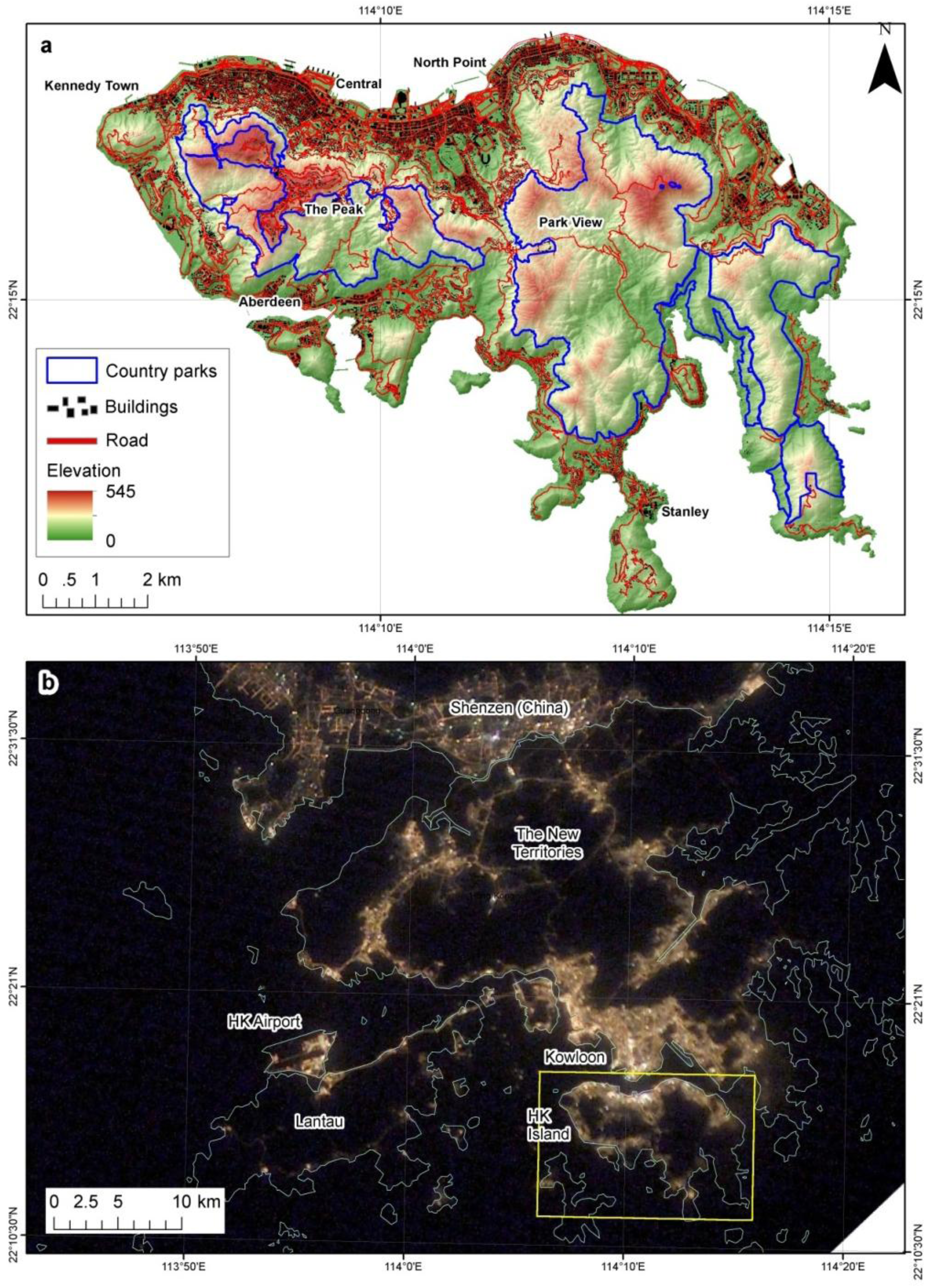
3.1. Study Area—Hong Kong Island

We demonstrate our approach using Hong Kong Island as an example. Hong Kong Island is one of the world’s economic centers, where high-density population is adjacent to non-built-up natural areas of rugged terrain. Although human settlements in Hong Kong can be dated back to the Neolithic Era [37], modern urban development on Hong Kong Island began in the late 1840s, following the first Opium War and the Treaty of Nanking in 1842. The Kowloon Peninsula and the New Territories were developed later, following the Convention of Peking in 1860 and the Second Convention of Peking in 1898, respectively [38]. Hong Kong’s population has grown steadily since the 1840s, reaching 1.6 million in 1939. The Second World War set back the population to 600,000 in the early 1940s. The population grew rapidly after the war and returned to the prewar population in just a couple of years [39]. Today, the Hong Kong Special Administrative Region is home to over seven million, making it one of the most densely populated places in the world (6,488 people/km2; [40]). The rapid growth of population and built-up areas during the 1960s raised the need for conservation of the countryside. In 1972, the Hong Kong Country Parks Program allocated nearly 40% of the Territory’s lands for conservation. These lands comprised mainly of mountainous landscape unsuited for urban development ([41]; Figure 1). A strong gradient in the intensity of human activity and of human impact on the environment takes place over very short distance in Hong Kong, due to its small land area, highly concentrated urban population, and rugged topography (as evident from the light pollution map; [42]; Figure 1).
Figure 1. Hong Kong Island study area (a). The bottom image (b) shows night-lights (an indicator for human activity) over the entire Special Administrative Region of Hong Kong as photographed from the International Space Station on 10 March 2003.
Land 02 00550 g001

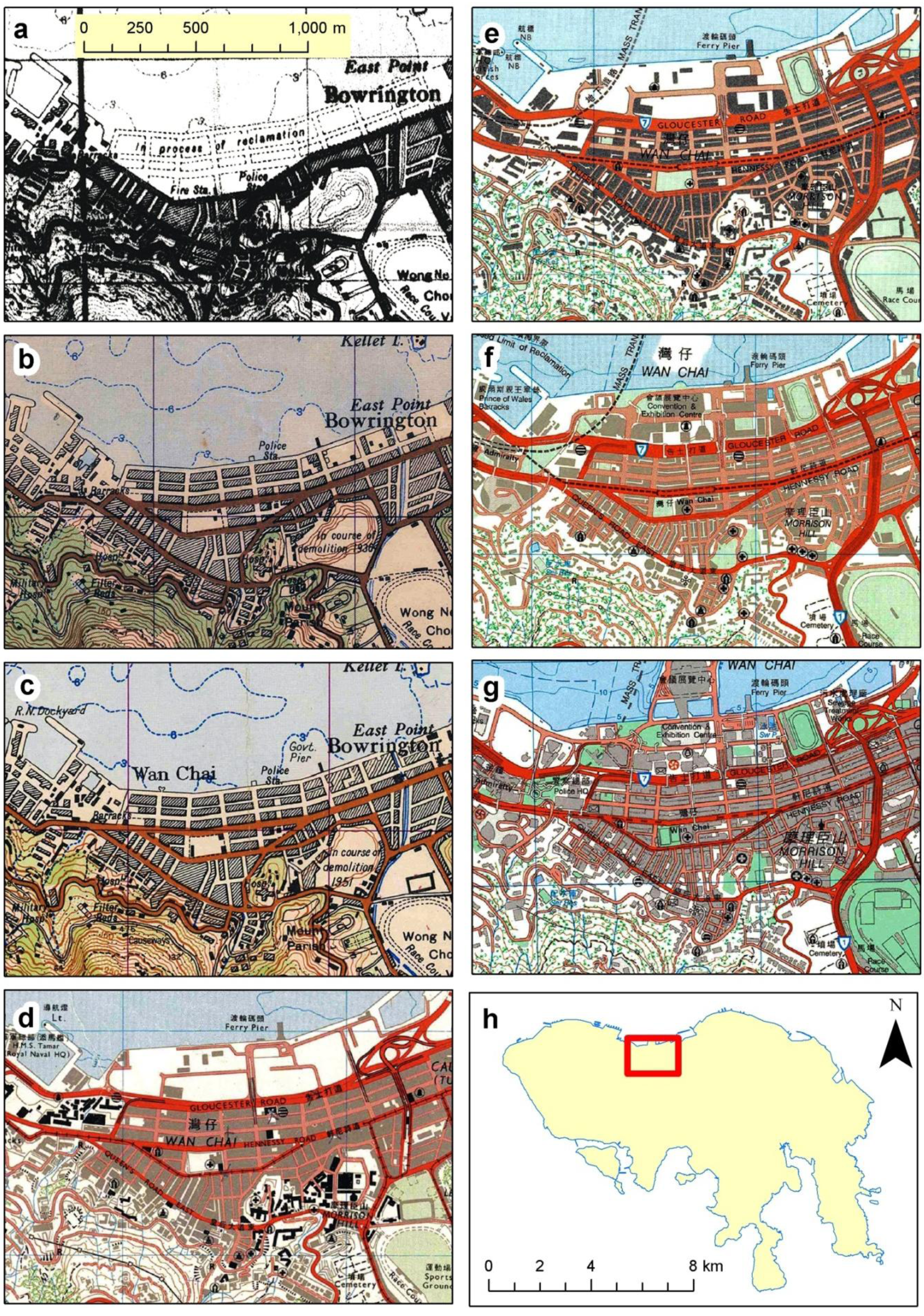
3.2. Historical Sources

To study changes in the built-up areas over time, we used historical topographic maps of Hong Kong Island, at the scale of 1:20,000, between 1930 and 2003/6 (Table 1; Figure 2). The maps were obtained from the Survey and Mapping Office of the Hong Kong Lands Department). They were first scanned and then georeferenced to the respective coordinate system used in each of the maps, as specified in Table 1. For the georeferencing process, several grid points were used, based on map graticules. The older maps (from 1930, 1945, and 1952) were georeferenced based on control points common to each of those dates and more recent maps. The root mean squared error in the georeferencing of the maps was below 0.5 mm (equivalent to less than 10 m on the ground) for most of the maps (Table 1). To correspond with the scale of the historical maps, all raster analyses reported below were performed at a spatial resolution of 10 m (i.e., 0.5 mm at a scale of 1:20,000).
Table 1. Historical maps (1:20,000) used in this study.
Historical MapSheetGeoreferencing Parameters
YearRMS Error (m)Projection NameDatum
1930Sheets 19 and 2313.05World Polyconic Grid HKD Clarke 1866
1945Northern Sheet-Sht. 197.46World Polyconic Grid HKD Clarke 1866
1945Southern Sheet-Sht. 236.36World Polyconic Grid HKD Clarke 1866
1952Northern Sheet-Sht. 199.90World Polyconic Grid HKD Clarke 1866
1952Southern Sheet-Sht. 234.35World Polyconic Grid HKD Clarke 1866
1975Northern Sheet-Sht. 113.81UTM50 InternationalD International 1967
1975Southern Sheet-Sht. 153.46UTM50 InternationalD International 1967
1984Northern Sheet-Sht. 112.98Hong Kong 1980 UTM Zone 50ND Hong Kong 1980
1984Southern Sheet-Sht. 153.07Hong Kong 1980 UTM Zone_50ND Hong Kong 1980
1995Northern Sheet-Sht. 113.29Hong Kong 1980 GridD Hong Kong 1980
1993Southern Sheet-Sht. 152.99Hong Kong 1980 GridD Hong Kong 1980
2003Northern Sheet-Sht. 112.84Hong Kong 1980 GridD Hong Kong 1980
2006Southern Sheet-Sht. 152.76Hong Kong 1980 GridD Hong Kong 1980

3.3. Reconstructing Historical GIS Layers of Built-Up Areas

We used 1:20,000 GIS vector layers (for the year 2006) of the roads, the buildings, the coastline and elevation contours, which were purchased from the Hong Kong Survey and Mapping Office as the base layers upon which we based our reconstruction of past GIS layers of built-up areas and roads. The process of editing the GIS layers was as follows. First, the GIS layers were fitted to the rectified maps of 2003/6, thus representing the state of the region for that period of time. Next, new layers were created by overlaying existing layers on maps from the previous period and modifying their attributes and geometry according to the details on those maps. For example, we laid the building layer of 2003/6 over the rectified maps of 1993/5 and created a new building layer for 1993/5 by changing the classification of each building according to the relevant maps (as in [12]). Thus, a building that existed in 2003/6 but did not exist in 1993/5 was marked as nonexistent in the 1993/5 layer, a building that appeared on the maps of 1993/5 but not on the 2003/6 layer was marked as destroyed and a building that exists both on the layer and on the map was marked in the 1993/5 as existent. This process was applied for each year on different layers of buildings, roads and the coastline. While individual buildings are not captured on the 1:20,000 Hong-Kong vector layers nor on the 1:20,000 topographic maps, these sources do show blocks of buildings, and that was the scale at which we mapped the built-up areas.
Figure 2. The historical 1:20,000 maps used for reconstructing the development stages of the Island of Hong Kong (showing the area of Wan Chai, in the north of Hong Kong Island): 1930 (a), 1945 (b), 1952 (c), 1975 (d), 1984 (e), 1993/5 (f), 2003/6 (g), location map (h). The maps reproduced with permission of the Director of Lands. © The Government of Hong Kong SAR. Licence No. 75/2013.
Land 02 00550 g002

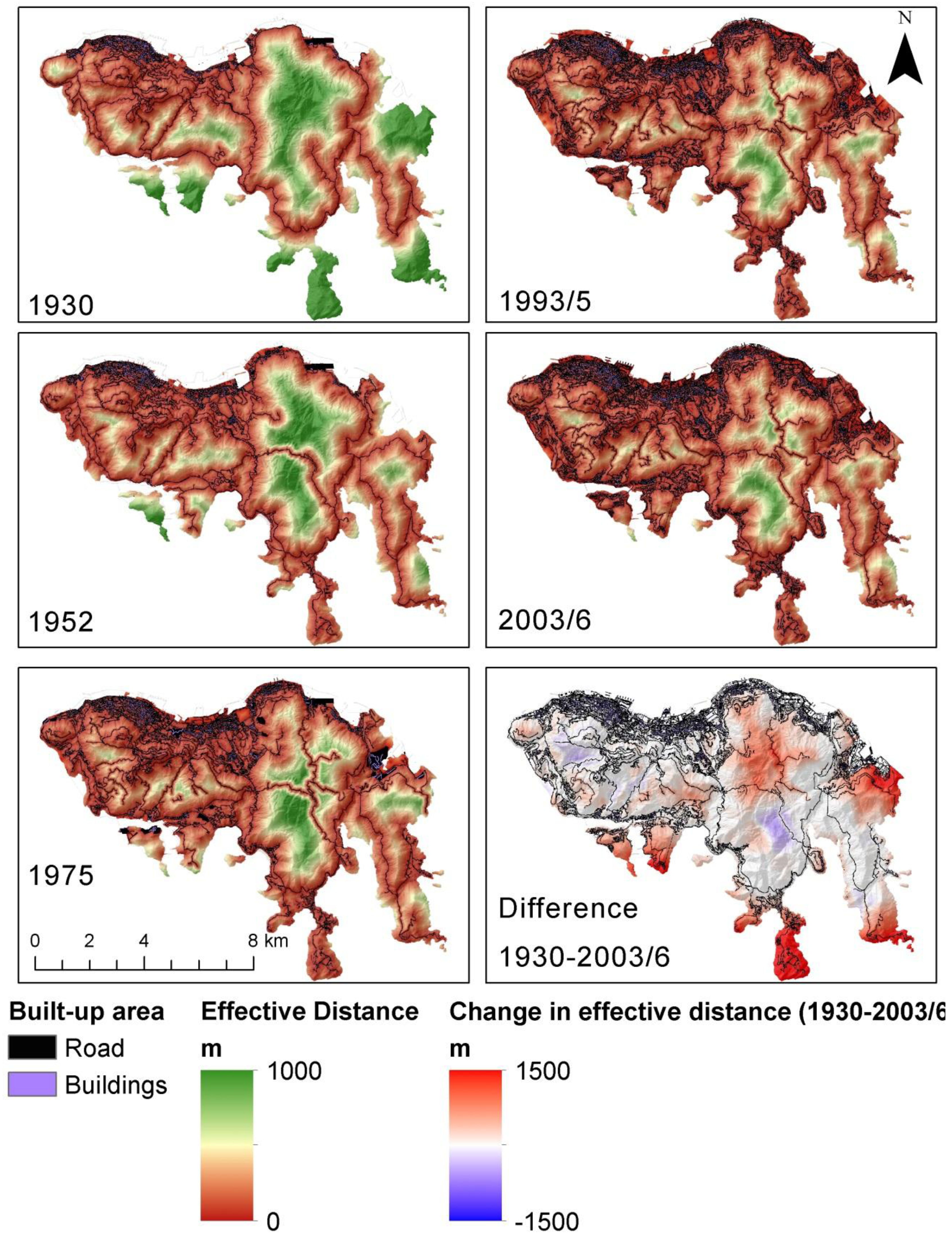
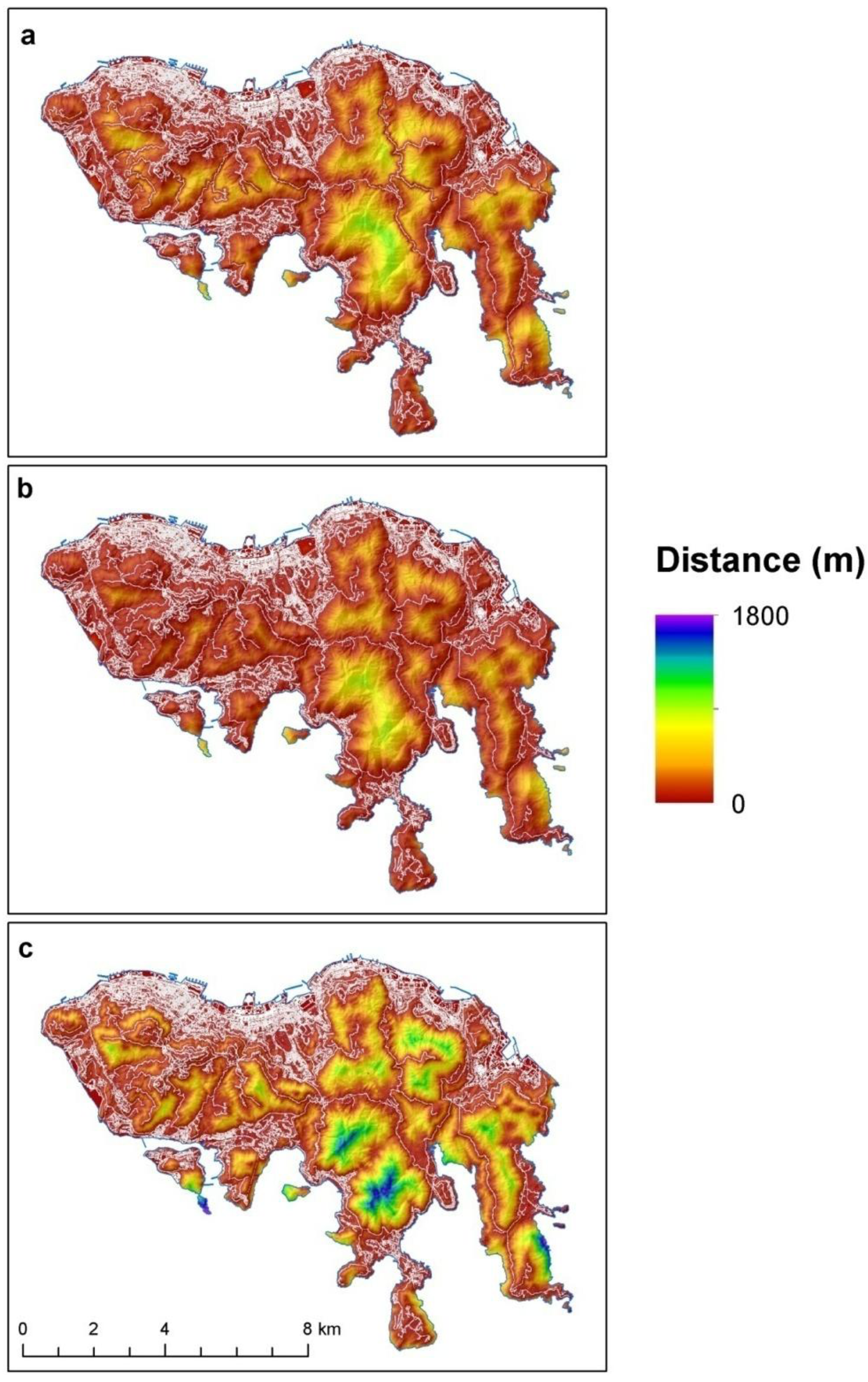
3.4. Landscape Continuity Analysis

We calculated landscape continuity using the approach developed by Levin et al. [6]. The landscape continuity value (LCV) at a certain pixel can be expressed by the following equation:
Land 02 00550 i001
where LCV is the landscape continuity value, Wn the weight (Table 2) assigned to the category n of a built-up area and Dn is the distance of a certain pixel from the nearest feature belonging to the category n of a built-up area. The units of LCV are therefore termed as a weighted distance or as an effective distance, and are given in meters or kilometers. The LCV can be summed over an area (to examine the total amount of landscape continuity; see [6]). Landscape continuity was calculated for each year separately so that changes over time could be examined. The weights of built-up area categories used are given in Table 2, based on expert estimation of relative environmental and ecological impacts of built-up areas categories (following the weights used by Levin et al., [6]). In addition, we had access to data on building height (i.e., approximate level of the top of a building in meters above the Hong Kong Principal Datum, SMO Geo-Reference Database, 2011 [43]. In some of our calculations we used building height values to assign weights for the categories of built-up areas. Higher buildings, indicating a larger number of people within a building, were assigned greater weights than lower buildings (Table 2). We further developed the landscape continuity model of Levin et al. [6] by assuming that the slope of the distance decay function of built-up areas depends not only on the type of built-up area, but also takes into consideration the topography of the area. This was done by applying a cost-distance analysis, in which the slope of the digital elevation model represented the cost of access, i.e., how difficult it is for people or domestic animals to gain access into open areas (as in [44]).
Table 2. Weights for different built-up areas and infrastructure categories, as applied in the landscape continuity value analysis.
Built-up Area TypeWeightEquivalent Distance of 1 km from a Large City
(km) = Reciprocal of the Respective Weight
Expressway100%1
Main road75%1.333
Secondary road (double width)50%2
Secondary road (single width)25%4
Built-up areas (without building height information)100%1
Building height less than 7.5 m75%1.333
Building height 7.5–15 m100%1
Buildings height 15–50 m125%0.8
Building height greater than 50 m150%0.666

3.5. Modeling Topographic Effects on the Landscape

Two classical topographic analyses in GIS include runoff and visibility. Runoff analysis is usually used either to generate the river network from a digital elevation model (DEM) (as in [45]), or to model runoff given specific rainfall, infiltration and land cover maps (as in [46]). We generated a DEM from contours (at vertical intervals of 20 m) at a spatial resolution of 10 m, using Idrisi GIS software [47]. Runoff originating from built-up areas and from roads may add pollutants to soil, wetlands, and water sources (as in [48]), thus impacting on biodiversity. We applied the runoff tool in Idrisi Taiga to model pollutants originating from built-up areas [47]. A runoff analysis calculates the accumulation of rainfall units per pixel based on topography. A simple runoff analysis accumulates rainfall on a per pixel basis as if one unit of rainfall was dropped on every location. We also assumed no drainage system was in place so each built-up pixel was used as a source of one unit of sewage. When incorporating building heights, the higher the building, the more sewage it would generate. While we acknowledge that Hong Kong does have high quality sewage and drainage systems, our aim in this model was to demonstrate this methodology. This particular parameter may be better suited to squatter communities than to proper cities or towns ([49]).
Visibility analyses are usually done for several applications, including military and environmental [44]. Our visibility analysis employed the VIEWSHED tool [47], using the proportional output option. The proportional output option produces an image in which the seen pixels are not assigned a boolean value of 1, but rather the value of the proportion of the viewpoints from which the pixel is seen. A pixel that is seen from only 1 of 10 input viewpoint pixels will have the value 0.1, for example, while a pixel seen from all 10 input viewpoints will have the value 1.0. We placed potential viewers in two settings: (1) in all buildings, to examine which open landscape areas are visible from the built-up areas? (2) Everywhere, i.e., if we randomly position viewers (n = 44,000, i.e., about 5 viewers/ha) throughout Hong Kong Island, to identify which areas would be the most visible, and which areas would be blocked (either by natural topography or by high buildings). In both settings, we analyzed the visibility with and without information about building heights, so as to demonstrate the effect that high-rise buildings have on the visibility of open areas (see [50]).

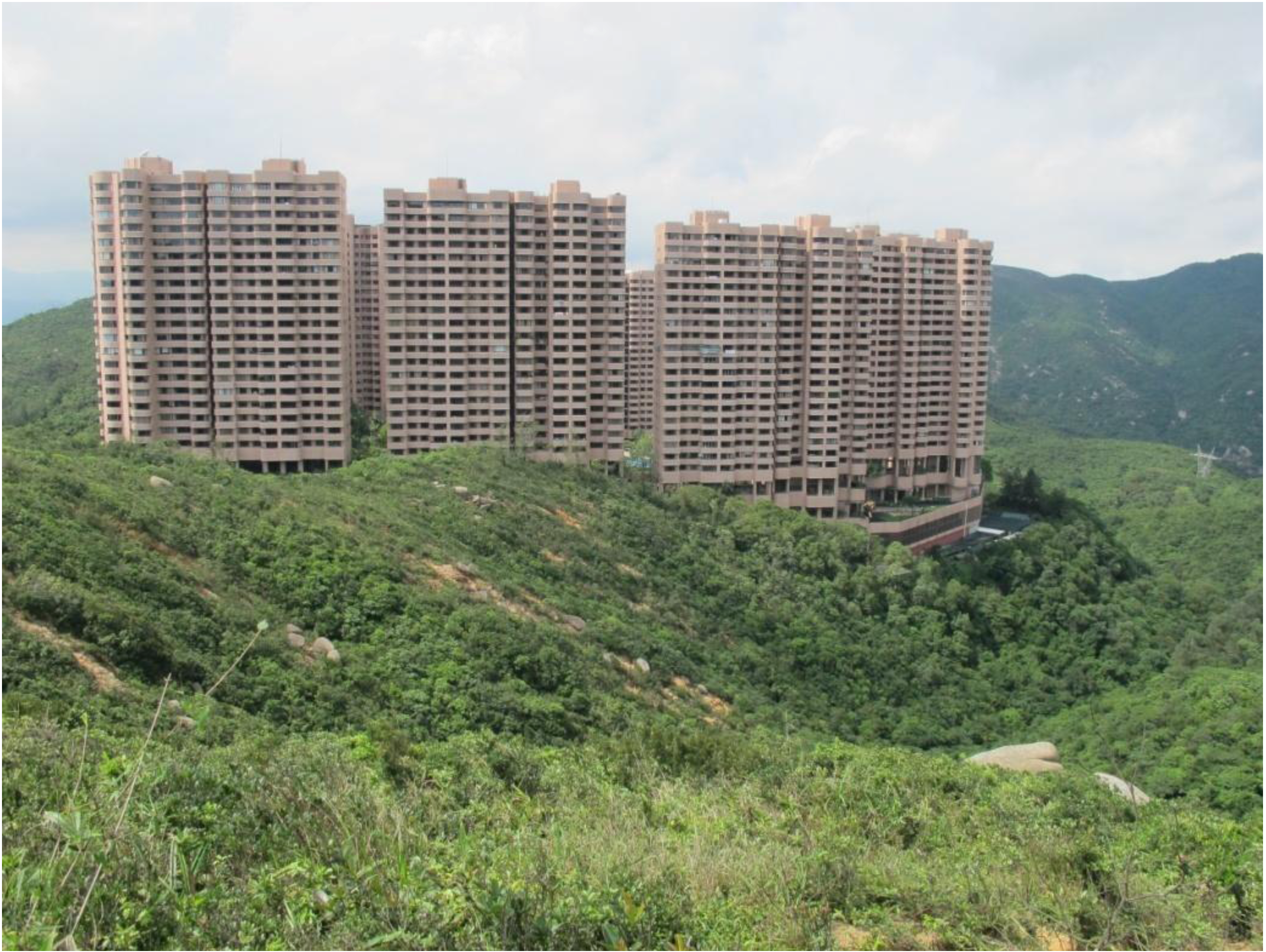
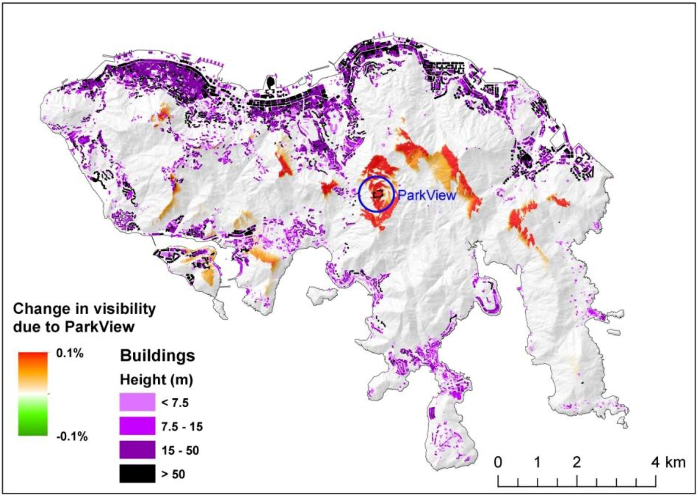
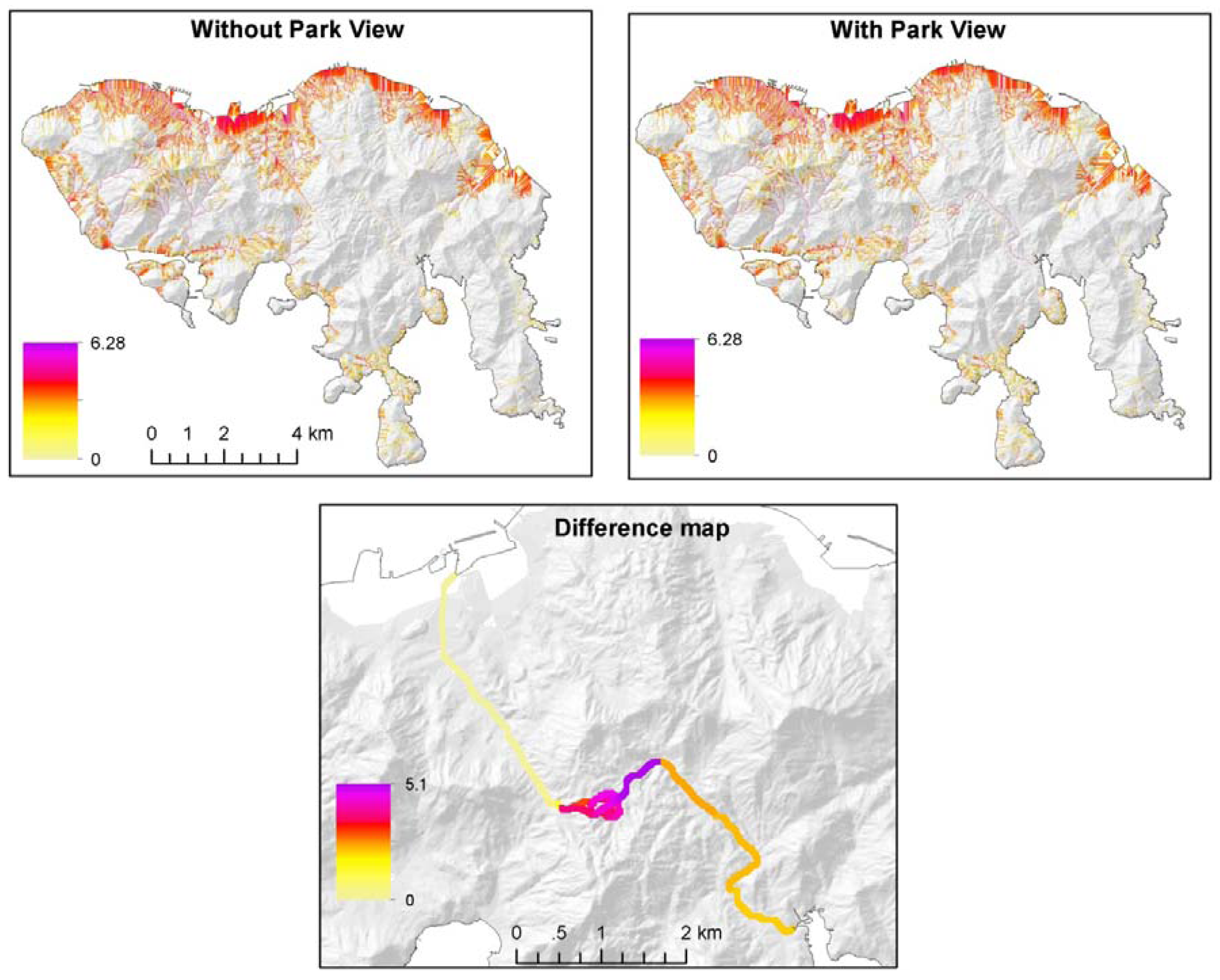
3.6. Case Study of Parkview Residential Project

As presented in Levin et al. [6], landscape continuity value maps can be used to estimate the potential impact of planned built-up areas, by calculating and mapping landscape continuity with and without a planned built-up area. Hong Kong Parkview is a residential project and a luxury tourist resort established in 1989 at the heart of Hong Kong Island, surrounded by the Tai Tam Country Park in the north, east, and south (Figure 3a and Figure 4). It consists of 18 blocks of residential buildings built on a ridge, 290–320 m above sea level. As described online [51], it is “Set on a hilltop separating the north and south side of the island, just inside 3,250 acres of the protected Tai Tam Country Park”. To demonstrate the use of the methods developed in this paper that incorporate topography for evaluating the effects of different planning scenarios, we calculated human impacts on the non-built-up areas with and without Parkview residential buildings (this was done for both the runoff and visibility analyses). We then subtracted the two layers of our modeled impacts with and without Parkview (as in [6]) to show which areas were affected by the construction of Parkview (in the results we will show this for the visibility and runoff analyses).
Figure 3. The reconstructed development stages of the Island of Hong Kong (between 1930 to the mid-2000s): Landsat false color image (a); land reclamation from the sea (b); development of the road network (c); and the development of built-up areas (d). The red rectangle in Figure 2a shows the location of Parkview residential project.
Land 02 00550 g003
Figure 4. Parkview residential project (photo taken by PC Lai, May 2013).
Land 02 00550 g004

4. Results

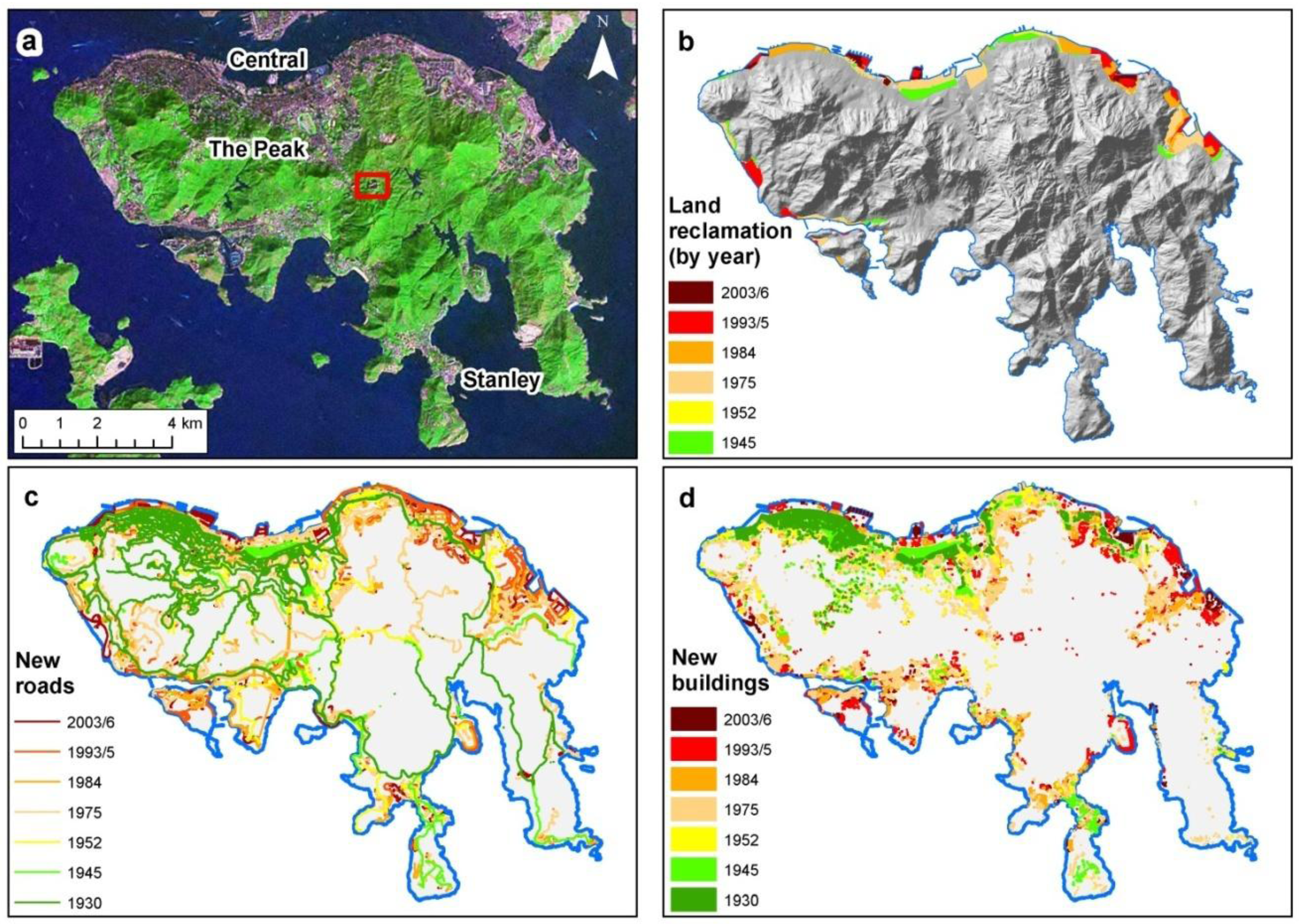
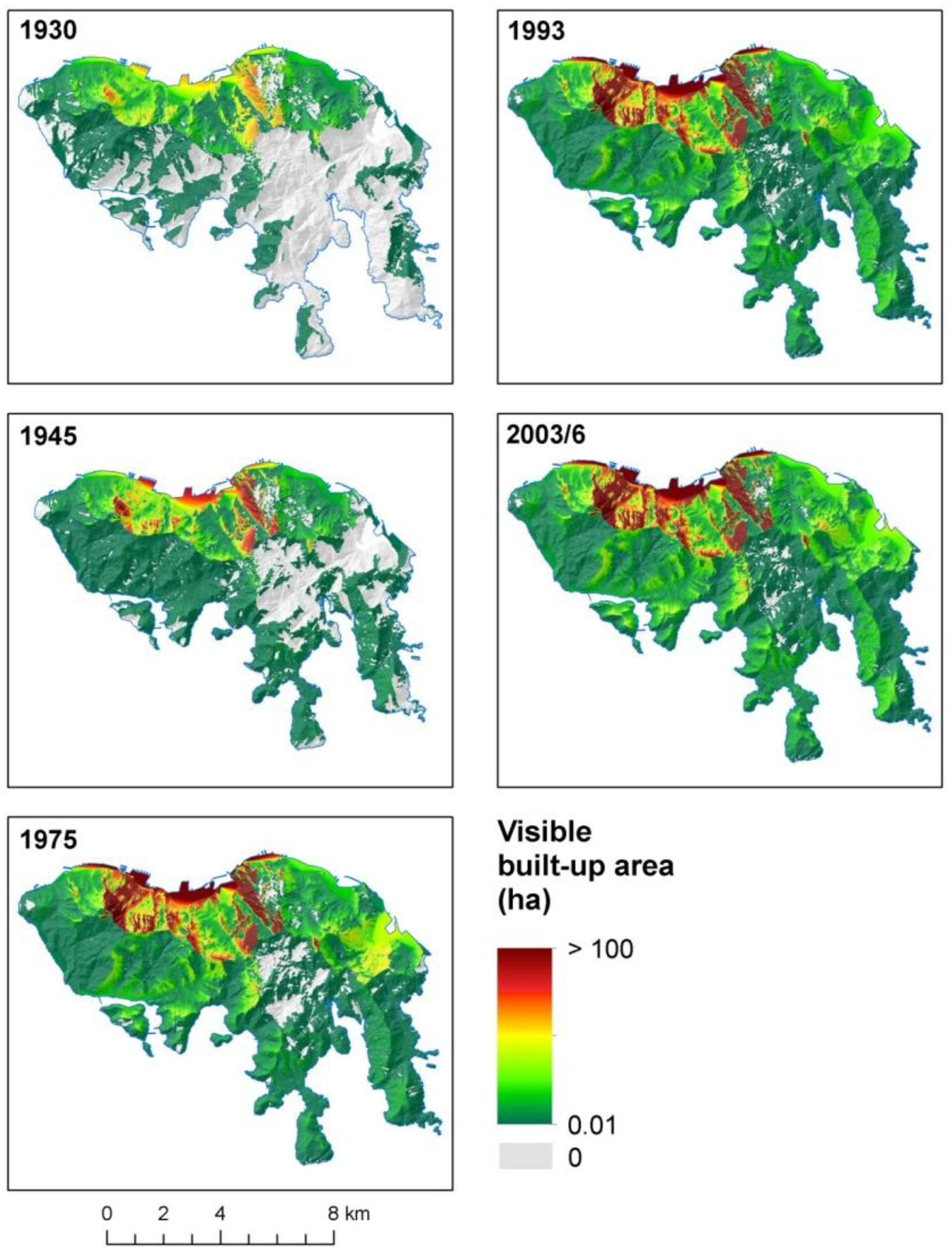
4.1. Temporal Changes in the Developed Areas

Based on the georeferenced historical maps we reconstructed the development stages of the Island of Hong Kong, examining three themes: land reclamation from the sea (Figure 3b), the development of the road network (Figure 3c), and the development of built-up areas (Figure 3d), between 1930 to the mid-2000s. As seen in these maps, the development of Hong Kong Island was constrained by the rugged topography on the one hand, and by the sea on the other hand. Land reclamation has been more extensive in the northern parts of the island, where the population density is high and suitable building land is scarce (Figure 3b). The built-up areas increased from 12,856 ha in 1930 to 56,012 ha in 2003/6, the percentage of the built-up areas increased from 1.7% in 1930 to 7% in 2006, while the total distance from roads and built-up areas has decreased (Table 3). Interestingly, the population size of Hong Kong Island has not changed much since the 1970s (Table 3). The development of new roads and built-up areas led to a decrease in landscape continuity, most notable in the southern and eastern parts of the Hong Kong Island, where landscape continuity values in some places in the 2000s decreased to less than 5% of their 1930 values, mostly due to the development of new towns and roads in the eastern and southern parts of Hong Kong Island (Figure 5).
Table 3. Time series of selected variables analyzed in this study.
Year (as in Table 1)193019451952197519841993/52003/6
Land area (ha), HK Island747,120755,992755,603772,264786,044797,393801,371
Built-up area (ha), HK Island12,85618,55921,30147,85552,14251,61856,012
Built-up area (%), HK Island1.7%2.5%2.8%6.2%6.6%6.5%7.0%
Sum distance from roads/built-up (km), HK Island335.0215.5162.8101.6100.191.989.2
Sum weighted distance from roads/built-up (km), HK Island344.6243.2200.8151.5147.6124.6120.0
Population, HK Island 409,203
(1931)
No dataNo data1,089,5001,179,0001,312,6371,268,112
Population, HK total840,473
(1931)
750,0002,250,0004,360,0005,397,9006,035,4006,935,900
(2005)
As in the landscape continuity analysis different weights are assigned to distance from built-up area classes, the resulting distances are higher than when a Euclidian distance surface is calculated (compare Figure 6a,b). Incorporating topography in landscape continuity analysis can be done by using slopes as a friction factor, decreasing the accessibility from roads and built-up areas. By incorporating topography as a friction, distance values are increased (compare Figure 6b,c).
Figure 5. Changes in landscape continuity on Hong Kong Island. Five panels show landscape continuity values calculated based on the roads network and buildings (1930, 1952, 1975, 1993/5, 2003/6); the lower-right panel presents changes in landscape continuity between 1930 and 2003/6, with warm hues (positive values) signifying a decrease in landscape continuity over time (calculated by subtracting the 2003/6 effective distances layer from the 1930 effective distances layer).
Land 02 00550 g005
Figure 6. Comparing three distance surfaces from built-up areas and roads: weighted distance (landscape continuity values) (a), Euclidian distance (b), Euclidian cost-distance using slope as the friction surface (c).
Land 02 00550 g006

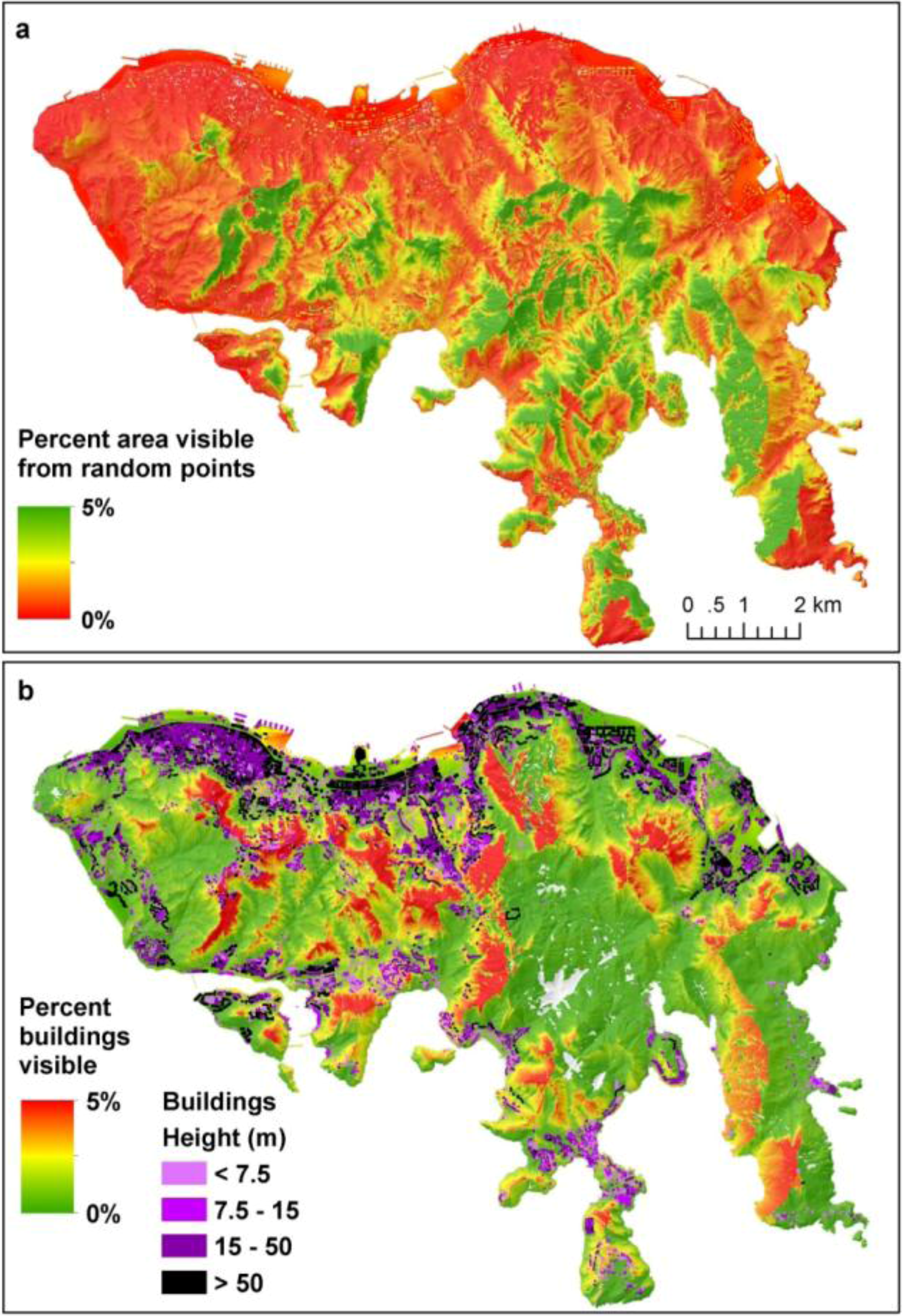
4.2. Viewshed Analysis

Examining changes in the visibility of built-up areas (i.e., to what degree are buildings seen from open spaces), we used the layers of the buildings (Figure 3d), and calculated the amount of the built-up areas visible from each pixel. In this analysis, information about the height of individual buildings was not incorporated (not available for past decades), and we assumed no obstructions by vegetation. As can be seen in Figure 7, visibility is mostly limited by watersheds and ridge lines. While in the northern part of HK Island, buildings command most of the view, in the southern part of the island, there are many areas where hardly any buildings were seen. However, this situation has changed over the past 80 years, due to the development of new towns and suburbs, and there are now hardly any areas from which no building can be seen (the grey areas in Figure 7). With time, there has been a decrease in the amount of areas in which people can experience wilderness (seeing no built-up areas), and there has been an increase in the total amount of built-up areas that are visible from the open landscape areas (Figure 7).
Figure 7. Changes in the visibility of built-up areas between 1930 and 2003/6. Values represent the amount of built-up areas visible from each 10 × 10 m grid cell (100 m2). In this analysis information about the height of individual buildings was not incorporated. Grey areas indicate areas from which no buildings were visible.
Land 02 00550 g007
A more realistic approach to analyze visibility is to include information about the heights of the buildings themselves. Two options exist to analyze the impact of building heights on visibility and on a “wilderness” experience, where views were not obstructed by tall buildings. First, we located 44,000 random observers, and calculated the percent area of Hong Kong Island visible from each pixel (Figure 8a); in this map, high values of observability are mostly found in the southern part of the island. Low values either result from obstruction by high buildings (as in the northern part of the island), or in peninsulas facing the sea, so that only small portions of the island can be seen from them. When the hypothetical observers are located on top of the roof of each building (Figure 8b), the analysis reveals in which areas a person is least likely to observe buildings, and can thus have a better “wilderness” experience; note that low values may be found also in low lying areas surrounded by buildings. Such an analysis can be used to demonstrate how development projects might change the visibility of open spaces. This can be done by calculating the visibility with and without a specific set of buildings, as in the case of the Parkview residential project, located in the middle of Hong Kong Island (Figure 9). Centrally located on a ridge line, the Parkview residential project can be seen from many places, and has therefore reduced the visibility of open spaces and has reduced the wilderness recreation experience in certain areas (Figure 9).
Figure 8. Visibility analysis taking into account building heights. In the upper map (a) visibility was calculated from a random sample of 44,000 points, and the map represents the percent area of Hong Kong Island visible from each pixel. In the lower map (b) visibility was calculated from the building roofs, and the map represents the percent of the buildings visible from each pixel.
Land 02 00550 g008
Figure 9. Changes in the visibility resulting from the construction of the Parkview residential project (in the middle of the island, in the blue circle). Areas where visibility of open spaces has decreased due to obstruction by the Parkview residential project are shown in orange-red colours.
Land 02 00550 g009

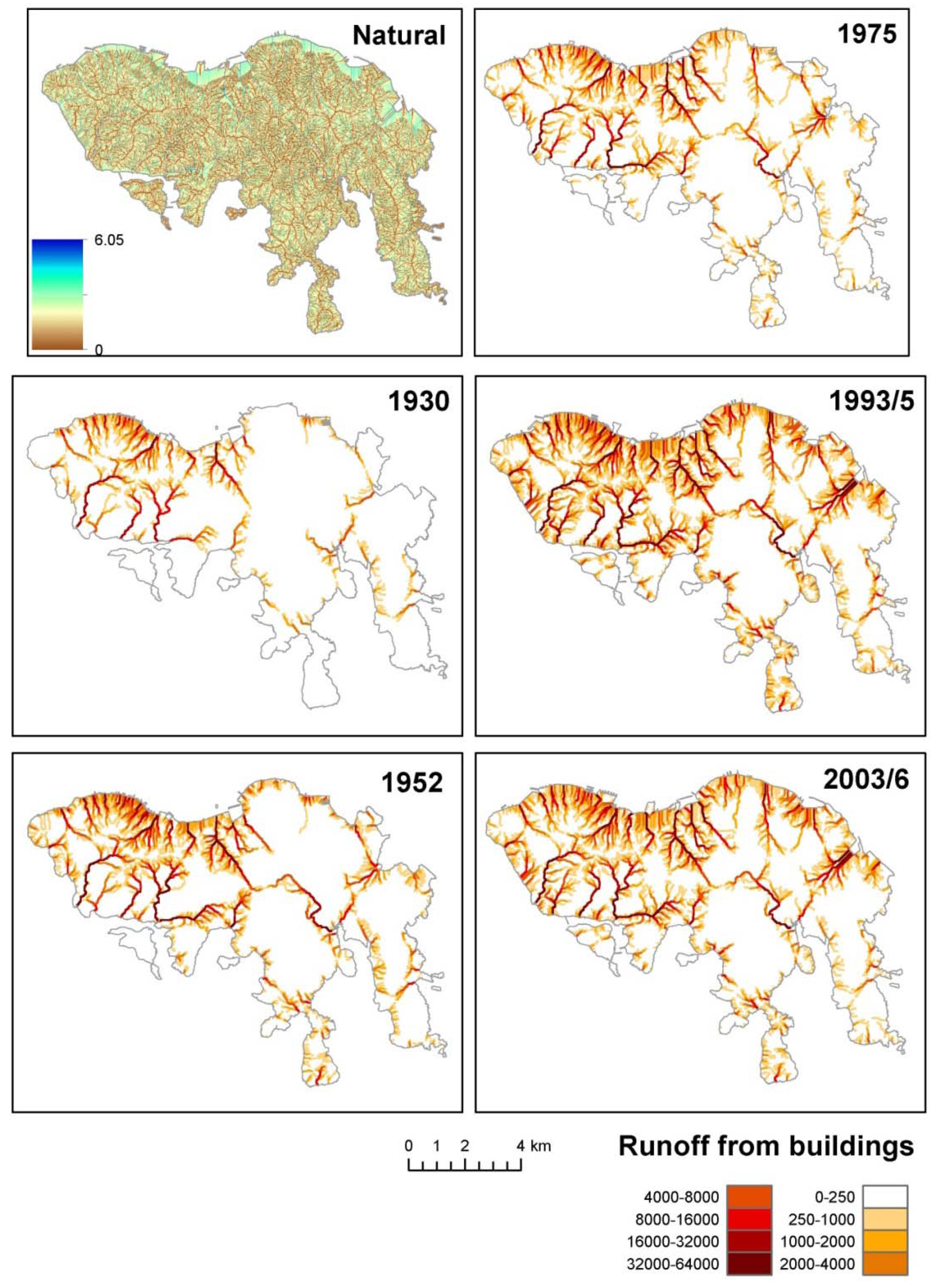
4.3. Runoff Analysis

A runoff analysis is commonly used to identify the natural drainage river network (Figure 10). Here we used this approach to model and visualize the cumulative runoff from buildings (assuming no urban drainage system for this demonstration, although the drainage system in Hong Kong is very extensive). With the development of new towns and suburbs on Hong Kong Island, more and more areas may be subject to runoff from built-up areas (Figure 10). The development of the Parkview residential project mostly affects runoff into the southern part of Hong Kong Island, but its impacts on runoff are spatially localized and limited to the riparian areas (Figure 11).
Figure 10. Runoff analysis—natural runoff assuming no buildings (upper left panel; values log transformed). Temporal changes in runoff from buildings, assuming no urban drainage systems, for the years 1930, 1952, 1975, 1993/5, and 2003/6. The values indicate the accumulated number of pixels contributing runoff to each pixel, based on the digital elevation model, and on the distribution of built-up areas.
Land 02 00550 g010
Figure 11. Changes in urban runoff due to the development of the Parkview residential project. The values indicate the accumulated number of pixels contributing runoff to each pixel, based on the digital elevation model, and on the distribution of built-up areas. Values were log transformed.
Land 02 00550 g011

5. Discussion

The development of new roads, buildings and neighborhoods affects open spaces surrounding these built-up areas in various ways. In this paper we aimed to demonstrate how human impacts on open spaces can be quantified and visualized, adding two additional dimensions to the commonly used planimetric analysis (x, y): the third dimension of height (z), and the fourth dimension of time (t). We quantified the development of built-up areas from historical topographic maps, and then analyzed how these temporal changes affected three human related variables: accessibility (modeled through the analysis of landscape continuity); [6]); visibility (i.e., the wilderness recreation experience, see [52]); and runoff. Quoting the ancient Greek philosopher Heraclitus, “Change is the only constant”, this is true not only for human life, but also for geographic phenomena. We used Hong Kong Island as a case study in this paper for three main reasons: the rapid transformations it went through during the 20th century, its varied topography, and the concentration of high-rise buildings adjacent to protected areas.
The way human activity and its impacts travel through space differ as a function of the type of human activity under consideration [6]. Building upon the three examples used here, we can classify human impacts based on three main dimensions:
  • Dispersion-concentration. While runoff tends to concentrate in rivers that converge, other impacts (e.g., air pollution, not analyzed here) tend to disperse with distance from the source.
  • Adjacency-remoteness. While runoff can only be transferred along continuous path ways, other impacts, e.g., visibility, may affect non adjacent areas, as a function of the topographic structure of the land.
  • Smoothness-steepness. While accessibility (as modeled through the landscape continuity analysis) tends to change gradually, other impacts, e.g., visibility, change their values abruptly, due to obstruction by ridge lines and high rise buildings.
A time series of maps showing the development of built-up areas enables the public to understand land cover changes. As some of our basic perceptions of nature and the environment are shaped in childhood, a phenomenon known as “environmental generational amnesia” [53,54] emerges, in which our baselines of what is natural shift with time as the environment undergoes degradation processes. We believe that maps such as we constructed in this paper may be instrumental in educating the public about the way our world looked before it became mostly urban. To this end we used historical maps that enable us to go back in time to decades when there were no aerial photos or satellite images available (as in [5,33]).
While we live in a three dimensional world, most of the maps we use portray it as two-dimensional, as we are mostly limited to the ground in our daily movement through space. Great efforts are invested in portraying topography on topographic maps [55]. However, not only is the natural environment topographically complex, the buildings we construct, most of all in the cities, create a new topography, ever breaking new heights [56]. While traditional landscape metrics assume that the underlying terrain is flat, there is in recent years an increasing recognition that to model landscape structure more realistically, the three dimensional nature of the world should be incorporated into landscape metrics, both in the patch-corridor-matrix model, e.g., [57] and in gradient representations of the surface roughness [58]. Using the approaches we demonstrated in this paper, we show that incorporating topography in our modeling of the impacts of built-up areas on open spaces, some areas may become less accessible to reach, but may still be susceptible to other types of human impact (e.g., visual intrusiveness, the disruption of a wilderness recreation experience by the visibility of built-up areas from open spaces [59]).

6. Conclusions

Using Hong Kong Island as a case study, a dynamic world city, where development is rapid, and where high-rise buildings are adjacent to country parks, we demonstrated how the environmental implications of development plans on their surrounding open spaces can be examined in the third dimension of height, and in the fourth dimension of time (using historical maps). In order to apply the methods demonstrated in this paper for urban planning issues, we recommend that information about building heights be incorporated to analyze the impacts of urban development projects on the surrounding open spaces. While, in the past, such information was not available, developments in remote sensing technologies and methodologies now make it easy to generate information on building heights (when not available as GIS layers), using diverse methods ranging from LiDAR [60], high spatial resolution sensors (as in [61] or aerial photogrammetry [62]. For future development plans, buildings’ heights may be extracted from town and architects’ plans. The analysis of the historical development of urban areas is now becoming easier to accomplish with developments in the field of historical GIS [63]. The Atlas of Urban Expansions is one such example of a database offering historic maps of the development of cities in the past 200 years [64,65].While it is important to understand landscape values and wilderness experiences using questionnaires and in-depth interviews (as in [59,66]), the methods developed here enable to quantify, model, and map the impacts of built-up areas on their surrounding open spaces, offering a powerful tool to inform people about present and future impacts. Through the examples in this paper we wish to encourage urban and environmental planners to incorporate topography (both natural and artificial) and historical perspectives, into their environmental impact analyses.

Acknowledgments

This research was partly supported by a grant from the The Louis Frieberg Center for East Asian Studies of the Hebrew University of Jerusalem. We are indebted to the Department of Geography at the University of Hong Kong for access to relevant map data for this research. We thank Leonie Seabrook for editing the manuscript. We thank the three anonymous reviewers whose suggestions helped improve the clarity of the manuscript.

Conflicts of Interest

The authors declare no conflict of interest.

References

  1. Sanderson, E.W.; Jaiteh, M.; Levy, M.A.; Redford, K.H.; Wannebo, A.V.; Woolmer, G. The human footprint and the last of the wild: The human footprint is a global map of human influence on the land surface, which suggests that human beings are stewards of nature, whether we like it or not. BioScience 2002, 52, 891–904. [Google Scholar] [CrossRef]
  2. Costanza, R.; d’Arge, R.; de Groot, R.; Farber, S.; Graso, M.; Hannon, B.; Limburg, K.; Naeem, S.; O’Neill, R.V.; Paruelo, J.; et al. The value of the World’s Ecosystem Services and Natural Capital. Nature 1997, 387, 253–260. [Google Scholar] [CrossRef]
  3. Li, C.; Lau, A.H.; Mao, J.; Chu, D.A. Retrieval, validation, and application of the 1-km aerosol optical depth from MODIS measurements over Hong Kong. IEEE Trans. Geosci. Remote Sens. 2005, 43, 2650–2658. [Google Scholar] [CrossRef]
  4. Lam, K.C.; Ma, W.C. Road traffic noise exposure in residential complexes built at different times between 1950 and 2000 in Hong Kong. Appl. Acoust. 2012, 73, 1112–1120. [Google Scholar] [CrossRef]
  5. Levin, N.; Elron, E.; Gasith, A. Decline of wetland ecosystems in the Coastal Plain of Israel during the 20th century: Implications for wetland conservation and management. Landsc. Urban Plan. 2009, 92, 220–232. [Google Scholar] [CrossRef]
  6. Levin, N.; Lahav, H.; Ramon, U.; Heller, A.; Nizry, G.; Toar, A.; Sagi, Y. Landscape continuity analysis: A new approach to conservation planning in Israel. Landsc. Urban Plan. 2007, 79, 53–64. [Google Scholar] [CrossRef]
  7. Giridharan, R.; Ganesan, S.; Lau, S.S.Y. Daytime urban heat island effect in high-rise and high-density residential developments in Hong Kong. Energ. Build. 2004, 36, 525–534. [Google Scholar] [CrossRef]
  8. Brezonik, P.L.; Stadelmann, T.H. Analysis and predictive models of stormwater runoff volumes, loads, and pollutant concentrations from watersheds in the twin cities metropolitan area, Minnesota, USA. Water Res. 2002, 36, 1743–1757. [Google Scholar] [CrossRef]
  9. Levin, N.; Duke, Y. High spatial resolution night-time light images for demographic and socio-economic studies. Remote Sens. Environ. 2012, 119, 1–10. [Google Scholar] [CrossRef]
  10. Sander, H.A.; Manson, S.M. Heights and locations of artificial structures in viewshed calculation: How close is close enough? Landsc. Urban Plan. 2007, 82, 257–270. [Google Scholar] [CrossRef]
  11. Jackson, S.D.; Griffin, C.R. A Strategy for Mitigating Highway Impacts on Wildlife. In Wildlife and Highways: Seeking Solutions to an Ecological and Socio-Economic Dilemma; Messmer, T.A., West, B., Eds.; The Wildlife Society: Nashville, TN, USA, 2000; pp. 143–159. [Google Scholar]
  12. Orenstein, D.E.; Bradley, B.A.; Albert, J.; Mustard, J.F.; Hamburg, S.P. How much is built? Quantifying and interpreting patterns of built space from different data sources. Int. J. Remote Sens. 2011, 32, 2621–2644. [Google Scholar] [CrossRef]
  13. Lake, I.R.; Lovett, A.E.; Bateman, I.J.; Langford, I.H. Modeling environmental influences on property prices in an urban environment. Comput. Environ. Urban 1998, 22, 121–136. [Google Scholar] [CrossRef]
  14. Mcgarigal, K.; Cushman, S.A.; Neel, M.C.; Ene, E. FRAGSTATS: Spatial Pattern Analysis Program for Categorical Maps; Landscape Ecology Lab, University of Massachusetts: Amherst, MA, USA, 2000. [Google Scholar]
  15. Tian, Y.; Jim, C.Y.; Tao, Y.; Shi, T. Landscape ecological assessment of green space fragmentation in Hong Kong. Urban For. Urban Green. 2011, 10, 79–86. [Google Scholar] [CrossRef]
  16. Leyequien, E.; Verrelst, J.; Slot, M.; Schaepman-Strub, G.; Heitkönig, I.; Skidmore, A. Capturing the fugitive: Applying remote sensing to terrestrial animal distribution and diversity. Int. J. Appl. Earth Observ. Geoinfor. 2007, 9, 1–20. [Google Scholar] [CrossRef]
  17. Hanski, I. Habitat connectivity, habitat continuity, and metapopulations in dynamic landscapes. Oikos 1999, 87, 209–219. [Google Scholar] [CrossRef]
  18. Kienast, F. Analysis of historic landscape patterns with a geographical information system—A methodological outline. Landsc. Ecol. 1993, 8, 103–118. [Google Scholar] [CrossRef]
  19. Tischendorf, L.; Fahrig, L. On the usage and measurement of landscape connectivity. Oikos 2000, 90, 7–19. [Google Scholar]
  20. Tischendorf, L.; Fahrig, L. On the use of connectivity measures in spatial ecology. A reply. Oikos 2001, 95, 152–155. [Google Scholar]
  21. Beier, P.; Noss, R.F. Do habitat corridors provide connectivity? Conserv. Biol. 1998, 12, 1241–1252. [Google Scholar] [CrossRef]
  22. Stein, J.L.; Stein, J.A.; Nix, H.A. Spatial analysis of anthropogenic river disturbance at regional and continental scales: Identifying the wild rivers of Australia. Landsc. Urban Plan. 2002, 60, 1–25. [Google Scholar] [CrossRef]
  23. Krisp, J.M. Three-Dimensional visualization of ecological barriers. Appl. Geogr. 2004, 24, 23–34. [Google Scholar] [CrossRef]
  24. Kirca, S.; Altincekic, H.; Levin, N. Landscape continuity analysis as a tool for landscape planning: A case study in istanbul. Landsc. Res. 2013. [Google Scholar] [CrossRef]
  25. Landenberger, R.E.; Ostergren, D.A. Eupatorium rugosum (asteraceae) flowering as an indicator of edge effect from clearcutting in mixed-mesophytic forest. For. Ecol. Manag. 2002, 155, 55–68. [Google Scholar]
  26. Zheng, D.; Chen, J. Edge effects in fragmented landscapes: A generic model for delineating area of edge influences (D-AEI). Ecol. Model. 2000, 132, 175–190. [Google Scholar] [CrossRef]
  27. Hoechstetter, S. Enhanced Methods for Analysing. Landscape Structure: Landscape Metrics for Characterising. Three-Dimensional Patterns and Ecological Gradients; Rhombos-Verlag: Berlin, Germany, 2009. [Google Scholar]
  28. Liu, H.; Chan, J.C. An investigation of air-pollutant patterns under sea–land breezes during a severe air-pollution episode in Hong Kong. Atmos. Environ. 2002, 36, 591–601. [Google Scholar] [CrossRef]
  29. Nash, R. Wilderness and the American Mind; Yale University Press: New Haven, CT, USA, 2001; Volume 219. [Google Scholar]
  30. Borrie, W.T.; Birzell, R.M. Approaches to Measuring Quality of the Wilderness Experience. In Visitor Use Density and Wilderness Experience: Proceedings; Friedmund, W.A., Cole, D.N., Eds.; RMRS-P-20; USDA Forest Service Rocky Mountain Research Station: Fort Collins, CO, USA, 2001; pp. 29–38. [Google Scholar]
  31. Krause, C.L. Our visual landscape: Managing the landscape under special consideration of visual aspects. Landsc. Urban Plan. 2001, 54, 239–254. [Google Scholar] [CrossRef]
  32. Flinn, K.M.; Vellend, M.; Marks, P.L. Environmental causes and consequences of forest clearance and agricultural abandonment in Central New York, USA. J. Biogeogr. 2005, 32, 439–452. [Google Scholar] [CrossRef]
  33. Sanderson, E.W.; Brown, M. An ecological first look at the Manhattan landscape prior to Henry Hudson. Northeast Nat. 2007, 14, 545–570. [Google Scholar] [CrossRef]
  34. Radeloff, V.C.; Hammer, R.B.; Stewart, S.I. Rural and suburban sprawl in the U.S. Midwest from 1940 to 2000 and its relation to forest fragmentation. Conserv. Biol. 2005, 19, 793–805. [Google Scholar] [CrossRef]
  35. Lai, P.C.; Kwong, K.H.; Mak, A.S.H. Assessing the applicability and effectiveness of 3D visualization in environmental impact assessment. Environ. Plann. B 2010, 37, 221–233. [Google Scholar] [CrossRef]
  36. Bar-David, S.; Saltz, D.; Dayan, T.; Shkedy, Y. Using spatially expanding populations as a tool for evaluating landscape planning: The reintroduced persian fallow deer as a case study. J. Nat. Conserv. 2008, 16, 164–174. [Google Scholar] [CrossRef]
  37. Liu, S. An Outline History of Hong Kong; Foreign Languages Press: Beijing, China, 1997. [Google Scholar]
  38. Sparrow, G.W. City profile: Hong Kong. Cities 1988, 5, 127–136. [Google Scholar] [CrossRef]
  39. Geiger, F.; Geiger, T. Tales of Two City-States: The Development Progress of Hong Kong and Singapore; National Planning Association: Washington, DC, USA, 1973. [Google Scholar]
  40. Population Reference Bureau. 2011 World Population Data Sheet; Population Reference Bureau: Washington, DC, USA, 2012. Available online: http://www.prb.org/pdf11/2011population-data-sheet_eng.pdf (accessed on 14 October 2013).
  41. Jim, C.Y. The country parks programme and countryside conservation in Hong Kong. Environmentalist 1986, 6, 259–270. [Google Scholar] [CrossRef]
  42. Pun, C.S.J.; So, C.W. Night-Sky brightness monitoring in Hong Kong. Environ. Monit. Assess. 2012, 184, 2537–2557. [Google Scholar] [CrossRef] [Green Version]
  43. Geo-Reference Database. Available online: http://www.landsd.gov.hk/mapping/en/digital_map/common/feature/g1_mf.pdf (accessed on 14 October 2013).
  44. Bell, T.; Lock, G. Topographic and cultural influences on walking the Ridgeway in later prehistoric times. Nato Asi Ser. Life Sci. 2000, 321, 85–100. [Google Scholar]
  45. Tianqi, A.; Takeuchi, K.; Ishidaira, H.; Yoshitani, J.; Fukami, K. Development and application of a new algorithm for automated pit removal for Grid DEMs. Hydrolog. Sci. J. 2003, 48, 985–997. [Google Scholar] [CrossRef]
  46. Vazquez, R.F.; Feyen, J. Assessment of the effects of DEM gridding on the predictions of basin runoff using MIKE SHE and a modelling resolution of 600 m. J. Hydrol. 2007, 334, 73–87. [Google Scholar] [CrossRef]
  47. Idrisi GIS Taiga; Clark Labs, Clark University: Worcester, MA, USA, 2012.
  48. Lee, C.S.L.; Li, X.; Shi, W.; Cheung, S.C.N.; Thornton, I. Metal contamination in urban, suburban, and country park soils of Hong Kong: A study based on GIS and multivariate statistics. Sci. Total Environ. 2006, 356, 45–61. [Google Scholar] [CrossRef]
  49. Neuwirth, R. Shadow Cities: A Billion Squatters, a New Urban World; Routledge: New York, NY, USA, 2005; pp. 309–316. [Google Scholar]
  50. Yang, P.P.; Putra, S.Y.; Li, W. Viewsphere: A GIS-based 3D visibility analysis for urban design evaluation. Environ. Plann. B 2002, 34, 971–992. [Google Scholar] [CrossRef]
  51. Hong Kong Parkview. Available online: http://www.hong-kong-hotels.ws/hong-kong-parkview/location.htm (accessed on 14 October 2013).
  52. Kruger, S.C.; Rusworth, I.A.; Oliver, K. The Verification of Wilderness Area Boundaries as Part of a Buffer Zone Demarcation Process: A Case Study from the Ukhahlamba Drakensberg Park World Heritage Site. In Science and Stewardship to Protect and Sustain Wilderness Values: Ninth World Wilderness Congress Symposium, Merida, November 2009; Watson, A., Murrieta-Saldivar, J., McBride, B., Eds.; USDS Forest Service Rocky Mountain Research Station: Fort Collins, CO, USA, 2011; pp. 190–195. [Google Scholar]
  53. Kahn, P.H., Jr. Children’s Affiliations with Nature: Structure, Development, and the Problem of Environmental Generational Amnesia. In Children and Nature: Psychological, Sociocultural, and Evolutionary Investigations; Kahn, P.H., Jr., Kellert, S.R., Eds.; MIT Press: Cambridge, MA, USA, 2002; pp. 93–116. [Google Scholar]
  54. Miller, J.R. Restoration, reconciliation, and reconnecting with nature nearby. Biol. Conserv. 2006, 127, 356–361. [Google Scholar] [CrossRef]
  55. Collier, P.; Forrest, D.; Pearson, A. The representation of topographic information on maps: The depiction of relief. Cartogr. J. 2003, 40, 17–26. [Google Scholar] [CrossRef]
  56. Acuto, M. High-rise Dubai urban entrepreneurialism and the technology of symbolic power. Cities 2010, 27, 272–284. [Google Scholar]
  57. Hoechstetter, S.; Walz, U.; Dang, L.H.; Thinh, N.X. Effects of topography and surface roughness in analyses of landscape structure—A proposal to modify the existing set of landscape metrics. Landsc. Online 2008, 3, 1–14. [Google Scholar]
  58. Hoechstetter, S.; Walz, U.; Thinh, N.X. Adapting lacunarity techniques for gradient-based analyses of landscape surfaces. Ecol. Complex. 2011, 8, 229–238. [Google Scholar] [CrossRef]
  59. Collins, D.; Kearns, R. “It’s a gestalt experience”: Landscape values and development pressure in Hawke’s Bay, New Zealand. Geoforum 2010, 41, 435–446. [Google Scholar] [CrossRef]
  60. Maas, H.G.; Vosselman, G. Two algorithms for extracting building models from raw laser altimetry data. ISPRS J. Photogramm. Remote Sens. 1999, 54, 153–163. [Google Scholar] [CrossRef]
  61. Fraser, C.S.; Baltsavias, E.; Gruen, A. Processing of Ikonos imagery for submetre 3D positioning and building extraction. ISPRS J. Photogramm. Remote Sens. 2002, 56, 177–194. [Google Scholar] [CrossRef]
  62. Baillard, C.; Maıtre, H. 3-D reconstruction of urban scenes from aerial stereo imagery: A focusing strategy. Comput. Vis. Image Underst. 1999, 76, 244–258. [Google Scholar] [CrossRef]
  63. Ell, P.S. Cambridge Studies in Historical Geography #39. In Historical GIS: Technologies, Methodologies, and Scholarship; Gregory, I.N., Ell, P.S., Eds.; Cambridge University Press: Cambridge, UK, 2007. [Google Scholar]
  64. Parent, J.; Civco, D.L.; Blei, A.M. Atlas of Urban Expansion; Lincoln Institute of Land Policy: Cambridge, MA, USA, 2012. [Google Scholar]
  65. Atlas of Urban Expansion. Available online: http://www.lincolninst.edu/subcenters/atlas-urban-expansion/ (accessed on 14 October 2013).
  66. Beeco, J.A.; Hallo, J.C.; Baldwin, E.D.; McGuire, F.A. An examination of the guided night hiking experience in parks and protected areas. J. PARK Recreat. Adm. 2011, 51, 72–88. [Google Scholar]

