1. Introduction
Large areas of grassland in semiarid/arid parts of the southwestern United States and northern Mexico are yielding to low-density, non-urban housing. In the United States, exurban land use occupies five to seven times more area than land with urban and suburban densities, and has increased at a rate of about 10%–15% per year [
1,
2]. The drivers of exurbanization are numerous [
3,
4], and include technological advancements and increases in tele-commuting [
5], transportation and road-network improvements [
6], and push (crime, crowding, poor education systems,
etc.) and pull (affordable or desirable housing, privacy, better schools,
etc.) factors [
3]. The rapid and dispersed nature of exurban development raises numerous ecological concerns, including reduction of water availability to biota due to ground water withdrawals, habitat fragmentation, disrupted fire regime, disruption of trophic linkages, and change in vegetation owing to invasive species [
7,
8,
9,
10]. Those same natural-resource amenities that attracted an influx of humans are often degraded by increases in housing and associated development.
The per capita land conversion in exurban areas is much greater than in urban locations [
11,
12], which has profound implications for regional biological diversity and ecosystem function. Theobald [
2] found that development patterns that are contiguous, of high density, and less dispersed have reduced overall effects on natural resources. The reduced effect on natural resources comes from smaller footprints or “disturbance zones”, lower percentage of impervious surfaces, and reduced pollution because fewer vehicle miles are generated. Exurban growth displays the opposite development pattern, suggesting a greater impact on natural resources. Some types of human activity, such as mono-crop agriculture and urban uses, affect broad expanses of the landscape and result in land-cover conversion that can be readily detected through remote sensing. These activities are typically well documented through land-cover maps. However, low-intensity land uses, such as low-density rural development, are more difficult to discern through land-cover assessments. This form of development is therefore more challenging to map and is typically not included in land-cover data [
1,
13]. Given its important ecological implications, research is needed to improve our understanding of the patterns, rates, and extent of exurban development.
Despite the enormous potential impacts on ecosystem function arising from this wide-spread land-use change, exurbanization has received much less study than land-use change in suburban or urban areas [
9]. Where there have been attempts to quantify the impacts of exurbanization, the arguments have largely been inferred (e.g., more roads per house create a larger area of disturbance and therefore must have more impact) rather than being measured (e.g., an empirical comparison of the impacts of different housing-density classes on specific ecosystem processes) [
2,
3]. In this study, we examined the impacts of exurbanzation on three ecosystem function indicators and compared them to areas with rural and suburban housing densities. Three indicators were chosen to test trends in impact across multiple indicators for an area. The three indicators—fire hazard, water availability, and generalized distance effects of houses and roads—were employed to assess the impacts of exurbanization in southeastern Arizona; these indicators, as well as the specific research questions related to each, are discussed below.
Integral to management and planning efforts is an understanding of land-use changes on natural resources and ecological processes [
14]. Many exurbanites see themselves as stewards of the land and there is a strong, pervasive view that dispersed, low-density residential development is a conservation-compatible land use. Some of the benefits of exurban development, according to their residents, include preserving flora and fauna through nature watching, environmental education for children, a more solid appreciation of nature owing to proximity, and houses serving as buffers between nature and other land uses [
15]. An additional stewardship role is the funding of conservation efforts and helping to create, or return to, a natural-resource based economy that is non-extractive [
3]. By providing a comparison to suburban and rural housing-density classes, this research contributes to the discussion on whether exurbanization is a conservation-compatible land use. This study focuses on threats to ecosystem function in the Sonoita Plain, southeastern Arizona, and examines the effects, as well as the potential, for long-term biophysical degradation, of exurban development in a semiarid grassland of southwestern North America.
1.1. Study Area
The Sonoita Plain (696 km
2) lies in a predominantly semiarid grassland located in northwestern Santa Cruz County, Arizona, between the Santa Rita and Huachuca Mountains (31°32’–44’N/110°28’–44’W). Elevations range from about 1,100–1,600 m, while elevations of upland areas, especially the Canelo Hills in the south-central part of the study area, approach 2,900 m (
Figure 1). Land ownership is roughly 50% public (United States Forest Service, Bureau of Land Management, State Lands) and 50% private. The Sonoita Plain is largely characterized by desert grassland, plains grassland and desert scrub communities (501 km
2/72% of study area), with some riparian forest and riparian woodland communities along Cienega Creek in the northern part of the study area (22 km
2/3% of study area) [
16]. Dominant grasses are blue grama (
Bouteloua gracilis), black grama (
Bouteloua eriopoda), threeawn grasses (
Aristida species), wolftail grass (
Lycurus setosus), and plains lovegrass (
Eragrostis intermedia); herbs and shrubs include burrowed (
Ambrosia dumosa), groundsel (
Senecio vulgaris), copper leaf (
Acalypha wilkesiana), fleabane (
Erigeron divergens), malvastrum (
Malvastrum bicuspidatum), and creosote (
Larrea tridentate) [
17]. Upland regions ringing the central Plain are dominated by oak communities (172 km
2/25% of study area) [
16], while agricultural and developed areas (3 km
2/0.4% study area) are located near towns [
18]. Mean temperatures range from a January minimum of −2 °C to a June maximum of 33 °C (1971–2000), and average annual rainfall is 460 mm, with more than 50% occurring during the summer (July to September) monsoon [
19]. This location is acknowledged to be a prime example of high plain southwestern grassland [
17].
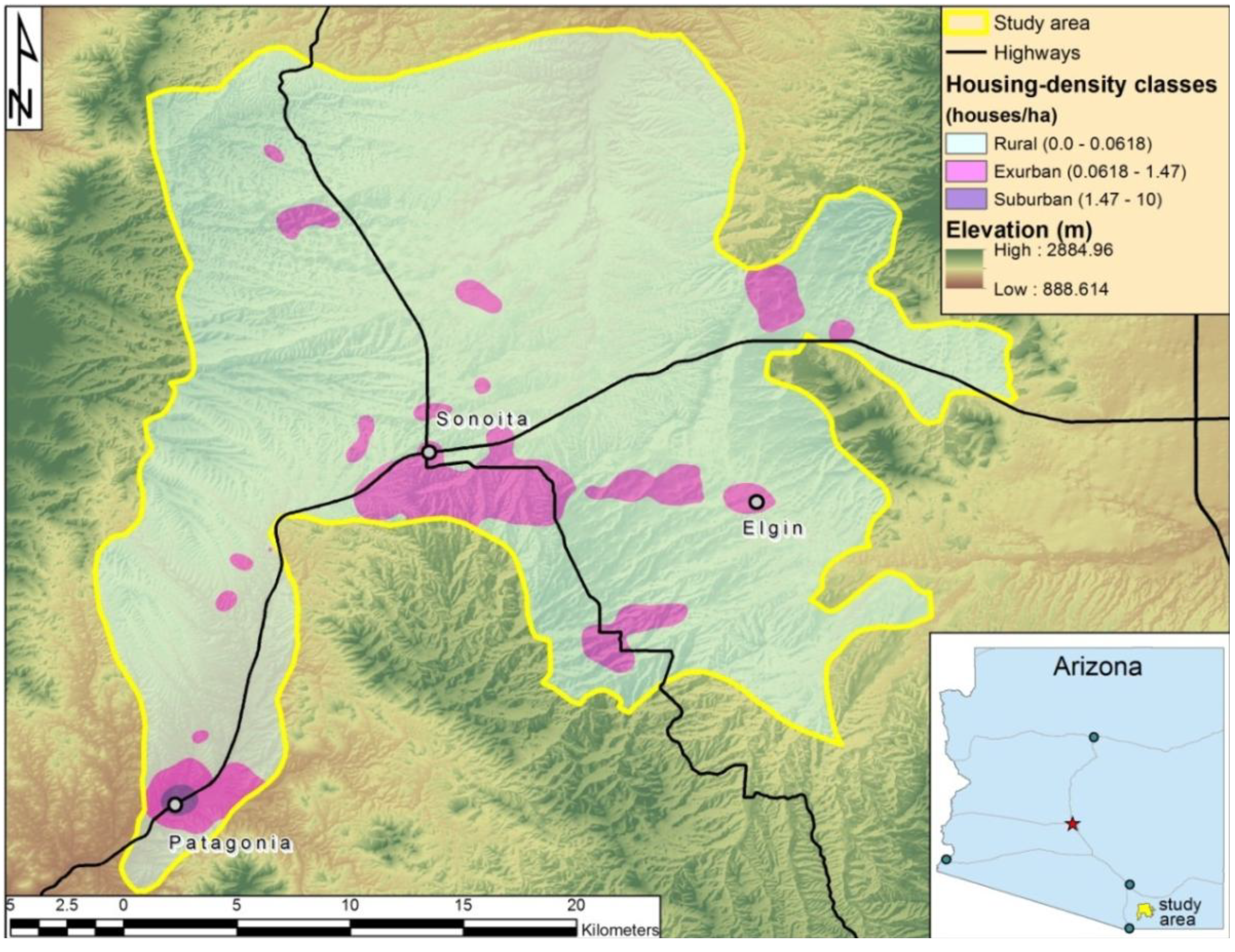
As the Sonoita Plain is entirely ringed by mountains, we delineated the study area to include the interior of the Plain using an impervious surface layer developed by the Water Resources Research Center, University of Arizona for the state of Arizona. The imperviousness of the substrate was selected as the defining study area characteristic because it has important consequences for the availability of water. Wells are mostly limited to the unconsolidated material of the Plain, with a handful of wells drawing water from shallow aquifers in the mountains. Given that ground water is the sole source of potable water in the area, this delineation corresponds well to human settlement in the area. The Sonoita Plain was classified as either pervious (unconsolidated material/soil) or impervious (rock) and the area inside the delineated “study area” outlined in
Figure 1 corresponds to unconsolidated material/soil. Here, “Sonoita Plain” and “study area” are used interchangeably to describe the interior of the Plain, as shown in
Figure 1.
Figure 1.
Housing-density classes in the Sonoita Plain, southeastern Arizona.
Figure 1.
Housing-density classes in the Sonoita Plain, southeastern Arizona.
In recent years, residential developments have sprung up on land historically used for cattle ranching. People are relocating to the Sonoita Plain in increasing numbers and houses are being constructed as vacation homes, retirement homes, and primary residences for those who commute to jobs in the nearby municipalities of Tucson, Nogales and Sierra Vista, Arizona. With 1,867 households and approximately 2,930 residents in 2010, the Sonoita Plain supports three different housing density classes, which makes it an ideal location to compare the impacts of exurban development to land use at other housing densities. Following previous work [
2,
20], the area contains rural housing densities (0–0.0618 unit/ha), exurban housing densities (0.0618–1.47 unit/ha), and suburban housing densities (1.47–10 unit/ha) (
Figure 1).
1.2. Indices of Ecosystem Function
1.2.1. Fire
Fire is critical to ecosystem health and stability across much of the United States, and the health of semiarid grasslands is particularly dependent on periodic burning. Fire ensures that fuel storage does not become excessive, helps maintain trophic connections, and prevents invasion by both native and exotic plant species [
21,
22]. However, decades of fire suppression have resulted in fires being largely excluded over a significant portion of the landscape for much of the twentieth century [
23]. These decades of fire suppression, combined with periodic climatic stresses and changing land-use patterns, have combined to produce highly hazardous conditions. The associated accumulation of fuels increases the probability of large, high-intensity wildfires and poses a threat to the long-term sustainability of these ecosystems [
24].
The increase in fire hazard is especially apparent in the western United States where rapid population growth, changing land tenures, and related increases in economic activity have contributed significantly to the nature and extent of fire risk. The wildlife-urban interface is expanding [
25], bringing people and structures in closer proximity to fire-prone environments and posing serious challenges to fire management. Exurbanization can alter fire frequency and promote intense fires owing to fire suppression and irrigation, which combine to increase the growth and storage of organic fuels. Natural fire frequencies for grasslands in southeastern Arizona have been estimated at between 10 and 20 years [
21,
22,
26,
27]; however, over the last 100 years, fire suppression has been largely successful, leading to few fires and leaving most areas unburned [
28,
29]. In this research, we examine whether there is a difference in fire risk between housing density classes.
1.2.2. Water
The semiarid grasslands of the Sonoita Plain maintain a delicate water balance. About 6%–7% (or approximately 13.6 × 10
6 m
3/yr) of the 43 cm of precipitation falling in upland areas contributes to aquifer recharge [
30]. Greatest depths to water generally are in uplands, whereas the shallowest ground water is near low-lying stream-corridor areas. Areas where depths to water are less than 20 m are underlain by thin deposits of unconsolidated alluvium, while upland areas, with large depths to water, are underlain by bedded rocks [
31,
32]. Disruption of recharge in uplands such as the Santa Rita Mountains, or pumping of water from wells at rates greater than the recharge rate, jeopardizes water availability in wells and the water required for ecosystem function. Over time, streams will dry up, riparian plant community composition will change, there will be less water available for wildlife, and residents will be forced to seek alternative sources of water [
33].
In this research, we investigated the depth to water and the number of wells, by housing-density class, to compare the impacts of exurbanzation on water availability to that of other housing-density classes. If the water withdrawal rates have started to deplete stored ground water, we would expect that depth to water in wells is greater where there are higher population densities. We might also expect that there are more new wells in exurban and suburban areas, which are experiencing rapid growth.
1.2.3. Generalized Distance Effects of Houses and Roads
Houses and roads have effects on ecological processes beyond their physical boundaries. In order to delineate generalized effects zones, the distances outward that the effects extend were taken into consideration. The “road-effects zone” concept has been introduced as an assessment and planning tool to synthesize diverse results (
i.e., separate patterns of interactions of roads with plants, animals, water, sediment, and other ecosystem characteristics) and detect overall patterns of how far road effects extend outward [
34]. We employed this concept to examine effects zones around both roads and houses. Some effects, such as mowing grass around houses, are immediately obvious, whereas others may manifest far off-site and substantially lagged in time, such as the slow transport of road-related pollutants into ground water systems. In general, effect zones extend further into grassland ecosystems than into forests [
34]. The full effects of road construction (restricted movement, increased mortality, habitat fragmentation, edge effects, invasion by exotic species, and increased human access to wildlife habitats) on biodiversity may be undetectable in some taxa for decades [
35]. As such, effects were divided into categories of “concentrated” and “diffuse” effects; reported literature values (
Table 1 and
Table 2, [
34,
36,
37,
38,
39,
40,
41,
42,
43,
44,
45,
46,
47,
48,
49,
50]) and aerial photography were synthesized and confirmed through personal observations in the study area, to generalize patterns of how far effect zones extend.
Table 1.
Concentrated-effect distances from roads for a range of factors impacting ecosystem services and processes. Adapted from Forman
et al. [
34].
Table 1.
Concentrated-effect distances from roads for a range of factors impacting ecosystem services and processes. Adapted from Forman et al. [34].
| Effects on Ecological Factors | Distance from Road Surface (m) | References |
|---|
| Roadside mowing | 0–25 | [34] |
| Earth-and-fill area formed by road construction equipment | 3–25 | [34] |
| Microclimate change | 10–40 | [34] |
| Direct mortality effects on animal populations | 2–15 | [34] |
| Seed germination inhibited | 12 | [34] |
| Habitat fragmentation (patch-size effects): carabid beetles | 1–20 | [49] |
| Rubber deposits from tires | 15–40 | [34] |
| Dioxins | 10–40 | [34] |
| Erosion and sedimentation caused by road construction | 30–50 | [36] |
| Heavy metals | 2–200 | [34,37] |
| Road density and decline in species abundance: amphibians | 1–200 | [38] |
| Traffic disturbance (noise, vibration, light): arthropod diversity | 40–55 | [34] |
| Traffic disturbance: attraction effect of light | 25–100 | [34] |
| Traffic disturbance: woodland birds near moderately busy road | 1–300 | [38,39,40,41] |
| Traffic disturbance: grassland birds near local road | 1–400 | [34,42,43] |
| Population depression (direct mortality): desert tortoise | 1–400 | [44] |
Table 2.
Diffuse-effect distances from roads for a range of factors impacting ecosystem services and processes. Adapted from Forman
et al. [
34].
Table 2.
Diffuse-effect distances from roads for a range of factors impacting ecosystem services and processes. Adapted from Forman et al. [34].
| Effects on Ecological Factors | Distance from Road Surface (m) | References |
|---|
| Erosion and sedimentation caused by road construction | 30–50 | [37] |
| Heavy metals | 2–200 | [34, 38] |
| Road density and decline in species abundance: amphibians | 1–200 | [39] |
| Traffic disturbance (noise, vibration, light): arthropod diversity | 40–55 | [34] |
| Traffic disturbance (noise, vibration, light): snakes | 150 | [50] |
| Traffic disturbance: attraction effect of light | 25–100 | [34] |
| Traffic disturbance: woodland birds near moderately busy road | 1–300 | [39,40,41] |
| Traffic disturbance: woodland birds near busy highway | 200–800 | [39,41] |
| Traffic disturbance: grassland birds near local road | 1–400 | [34,42,43] |
| Traffic disturbance: grassland birds near moderately busy road | 300–700 | [34,39,45,46] |
| Traffic disturbance: grassland birds near busy highway | 800–1,200 | [34,41,43,45,46,47] |
| Population depression (direct mortality): desert tortoise | 1–400 | [44] |
| Decline in species richness & decades-long lag-times in biodiversity loss: herptiles, birds, vascular plants | 1–200 | [35, 48] |
| Nitrogen levels and decline in species richness: amphibians | 1–2,000 | [38] |
| Habitat fragmentation/isolation, smaller populations, local extinction risk | 500–1,000+ | [36] |
| Disruption of wildlife movement corridors | 500–1,000+ | [34] |
| Invasion by roadside weeds & non–native species | 500–1,000+ | [34] |
Roads and houses can produce cumulative effects on animal populations [
44], hydrologic systems [
51], stream networks [
34], and other components of landscapes in which they are embedded. For example, where road networks are dense, the disturbance effects of traffic on bird populations may be compounded. Traffic noise constitutes a serious problem for breeding densities of some passerine birds [
40], and populations of many species of large wildlife, including wolves [
52,
53] and mountain lions [
34], only thrive where road density is less than 0.6 km/km
2. Similarly, branching road networks can fragment the landscape in a way that amplifies habitat fragmentation beyond the impact of a single road. The effects zones described above may not adequately consider these compounding effects. As such, we also attempted to provide a measure of the cumulative impacts of generalized distance effects by estimating the area surrounding each point on the landscape that is affected by the placement of roads and houses. These generalized distance effects, both separate and cumulative, were evaluated for each of the housing density classes.
1.3. Methods
Spatial analysis and modeling was conducted using ArcGIS v 10 (ESRI, Redlands, CA, USA). All maps were displayed in geographic-coordinate system, GCS North American 1983, datum D North American 1983; all analysis layers were projected to NAD 1983 UTM Zone 12N. The three indicators described above were compared by housing-density class.
1.3.1. Deriving Contextual Variables
It is common to measure the pattern and extent of development through population or population-density. However, population data from the US Bureau of the Census are tied to the primary residence and such measures can underestimate landscape changes because vacation and second homes are not represented. Therefore, housing density is a more complete and consistent measure of landscape change than population density [
2]. In lightly-settled landscapes, houses are not evenly distributed across large census blocks, and census-based housing-density measures do not capture real location distribution or settlement patterns. To address this, the locations of all houses in the Sonoita Plain study area were manually digitized from 2010 high resolution (1 m) aerial imagery obtained from the USDA Farm Service Agency, National Agricultural Imagery Program (NAIP). These locations were cross-checked against 2010 US Bureau of the Census data to ensure that the number of homes digitized in each census block matched the number of homes reported in the 2010 US Census. By digitizing the location of each house, a representation of how houses are distributed across the landscape emerges. Road information and town locations were obtained from 2010 census data (US Bureau of the Census) for Santa Cruz, Cochise, and Pima counties in Arizona. The elevation model used was the 1/3-arcsecond digital elevation model provided by the US Geological Survey [
54].
1.3.2. Fire
Efforts to protect ecosystem function require the development of wildfire-management plans. One way to inform fire management it through the use of historic fire data to determine areas that have gone without a fire longer than expected and are likely to be overloaded with fuel. The Fire Return Interval Departure (FRID) for an area is a metric derived from an inferred normal fire-return interval (the historical average, in years, between fires), and the elapsed years since the last fire [
55]. Maps of where and when fires have occurred in the past provide the foundation for calculating the average fire return intervals for each vegetation type class. A derived index can then be calculated for each map pixel, using the time that has elapsed since the last fire, to quantify the departure of an area from its average fire return interval [
55,
56]. The FRID index is: (Years since last fire—Natural Fire-return Interval)/Natural Fire-return Interval. FRID values for the Sonoita Plain are shown in
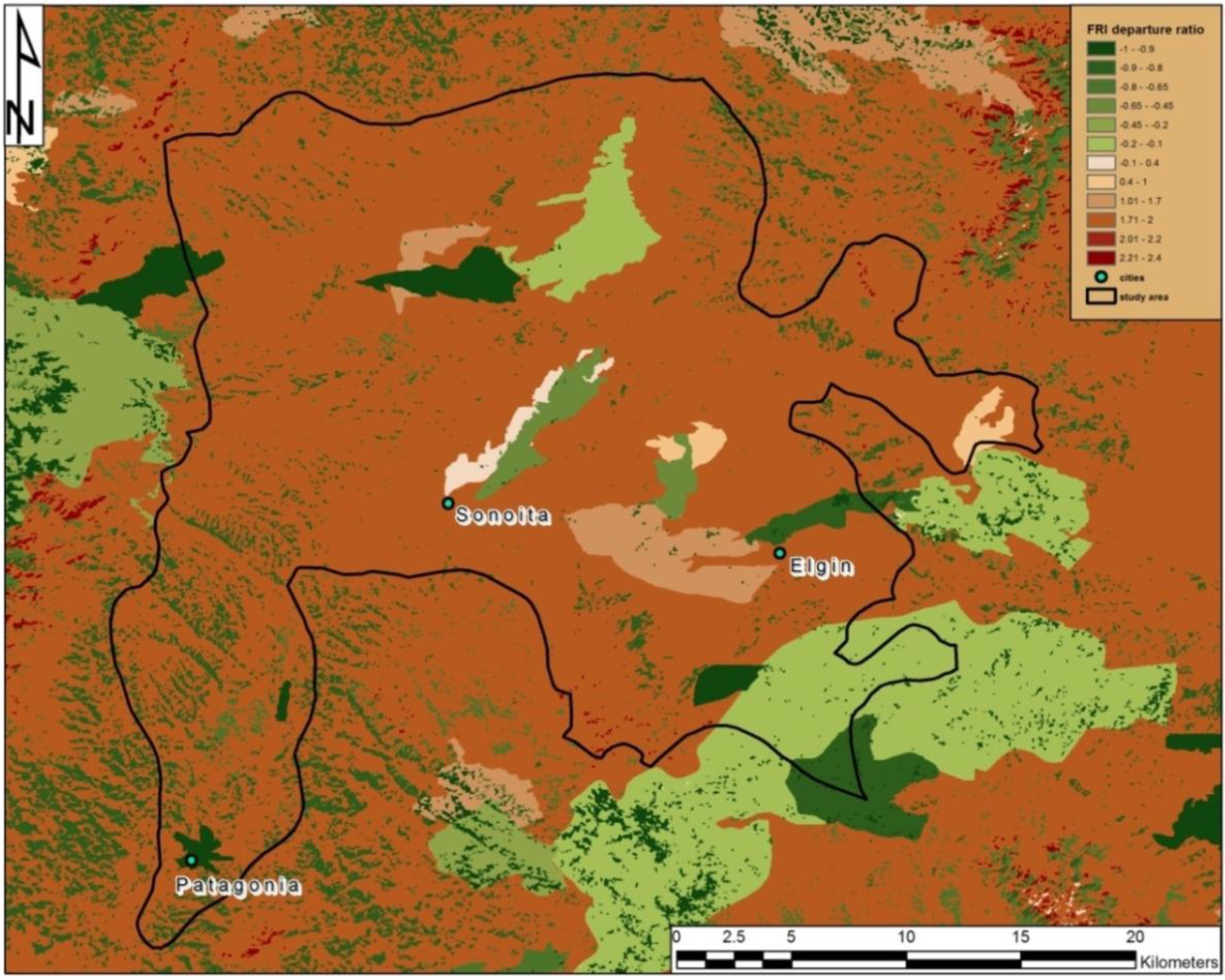
Figure 2. A positive index value indicates that the time since the last burn has exceeded historic fire return intervals. A negative index value indicates that the area has burned within its historic fire return interval. The FRID index does not consider fire severity.
Figure 2.
Fire Return Interval Departures (FRID) values for the Sonoita Plain, Arizona. Green represents low risk of fire, while reds and browns represent moderate to high risk.
Figure 2.
Fire Return Interval Departures (FRID) values for the Sonoita Plain, Arizona. Green represents low risk of fire, while reds and browns represent moderate to high risk.
Fire perimeters for the study area were compiled from 1984 to 2011. Fire perimeters for those fires that occurred from 2001 to 2009 and covered over 40.5 ha were compiled from the Wildland Fire Decision Support System [
57]. Older fires and those that burned less than 40.5 ha were compiled from the Monitoring Trends in Burn Severity (MTBS) project [
58]. MTBS covers 1984–2010 and the earliest fire in our study area obtained from this database occurred in 1985. The fire perimeters of the three 2011 fires were manually digitized from two Landsat images: one from Landsat 5 TM (path 35; row 38) on 11 March 2011 (bands 2, 4 and 7; 30-m resolution), and the second from Landsat 7 ETM+ (path 35; row 38) on 6 May 2011 (bands 2, 4 and 7; 30-m resolution). Using composite images, the burned areas were easily visible and were used to draw the fire perimeter.
Fire Return Intervals (FRI) values used match historic fire return intervals for Arizona and New Mexico [
59]. Where a range was given for the FRI, the average maximum was used in FRID calculations [
55]. Vegetation types used in the FRID calculations came from the Southwest Regional Gap Analysis Program (SWReGap) [
18] and were reclassified to match those corresponding to the FRI values [
59]. Riparian-zone and marsh vegetation FRIs were set to 10 years, as were those of the semi-desert grasslands that surround most riparian-zone locations in our study area. The FRIs of agricultural and developed areas were set to 500 years, as the objective is to prevent fires entirely in these areas. The number of years since last fire was calculated as (2011) minus (year of fire).
1.3.3. Water
Information about well location, well depth, water depth, and drill/registration date came from the Arizona Department of Water Resources Well Registry [
60]. Using the coordinates provided in the ADWR Well Registry, the locations of all registered wells in the Sonoita Plain were mapped; in cases where wells were re-registered, only the most recent registration was used. Average water depth for the study area was derived using the Kriging interpolation method from well points (100-m output cell; variable search radius with 36 points) [
61]. Water depths from all wells through 1970 were used to interpolate water level below land surface for 1970, whereas water depths from all wells registered from 2001 to 2010 were used to interpolate water level below land surface for 2010. Changes in water depth over 40 years were calculated as (2010 interpolated water level) minus (1970 interpolated water level). Where reported, drill date was used for the year, otherwise the application date was used.
1.3.4. Generalized Distance Effects of Houses and Roads: Concentrated Effects
Concentrated effects are those that are substantial or striking, but only extend a short distance beyond the house or the road. Examples include lawns and gardens, mowing of grass, outside areas accessible to pets, driveways, road shoulders, fences, and other infrastructure. Many of the significant effects from roads that are limited to short distances are due to particulates and aerosols deposited from local air movements. Some road effects involving species and the transfer of energy and materials also extend over short to medium distances (
Table 1). Roads were divided into highways and single-lane roads. Owing to their larger size and a larger cleared roadside area, ability to accommodate much greater volumes of traffic, and role as transportation corridors, highways were assigned larger effects zones than regular roads. The different effects of highways and roads are especially well illustrated in terms of traffic disturbance on bird populations (
Table 1 and
Table 2). The data presented in
Table 1 were used to derive a generalized concentrated-effects zone of 30 m for roads and 100 m for highways.
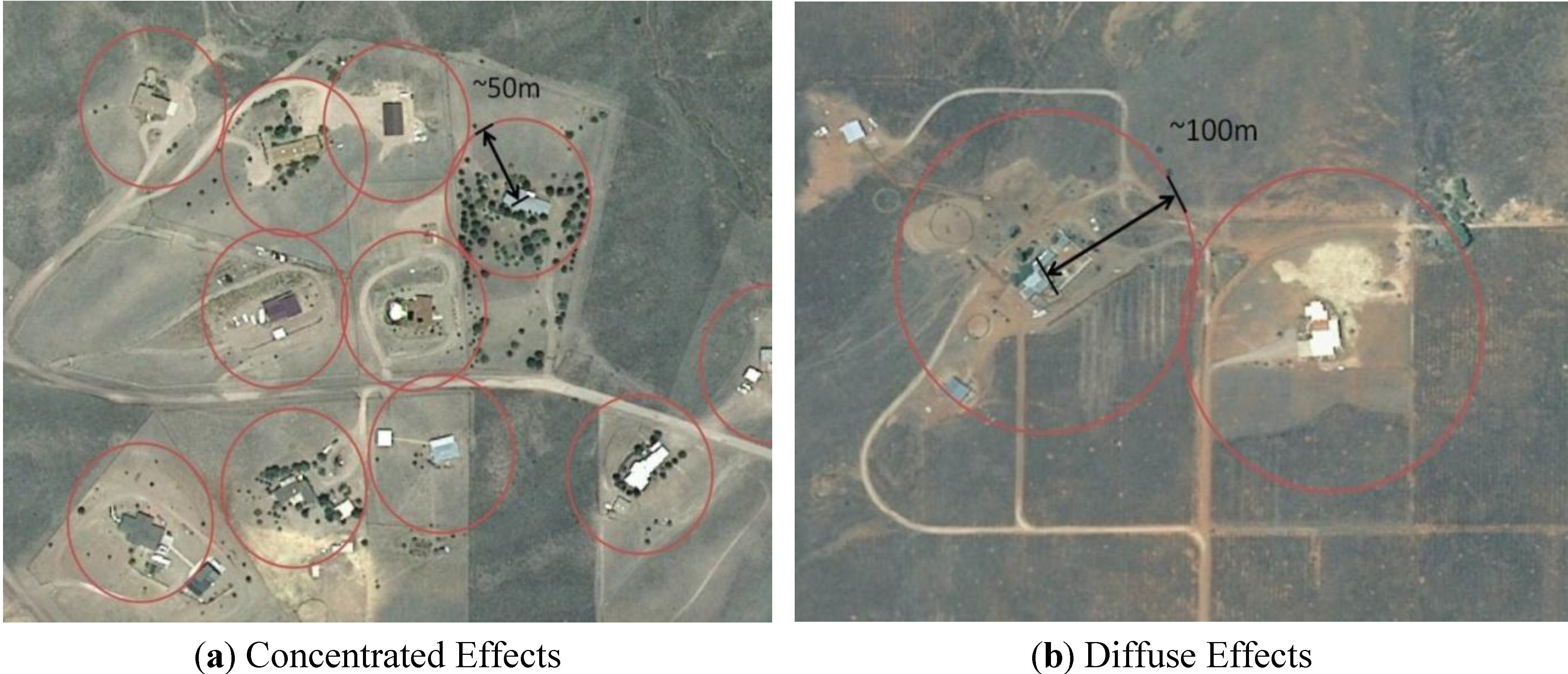
The concentrated effects of houses on ecological processes were directly estimated from 1-m NAIP images to extend 50 m outward from houses (
Figure 3). The concentrated-effects zone includes driveways, outbuildings, gardens, and mowed lawns, and represents intensive modification to the landscape. Some of the effects listed above for roads also apply to houses (e.g., microclimate change, inhibition of seed germination). In addition, sources of water found near houses can serve as oases in water-limited grassland systems, which can increase species diversity and abundance [
63]. On the other hand, pets can have detrimental effects on native species, especially ground-nesting birds. All of these modifications to the landscape have a concentrated effect on ecological processes. To visualize and measure the area of the concentrated-effects zones, buffers defined by the effects zones described above were created around each house, road, and highway in the study area.
1.3.5. Generalized Distance Effects of Houses and Roads: Diffuse Effects
Diffuse effects are effects on ecological processes that are more subtle than concentrated effects, and typically extend much further away from the house or road. Examples of diffuse effects include noise, chemical transport, erosion, and spread of invasive species (
Table 2). Most of the effects of roads that extend outward over longer distances involve human-access disturbances, exotic/invasive species spread, and the disruption of wildlife corridors. The data presented in
Table 2 were used to derive a generalized diffuse-effects zone for roads at 100 m and for highways at 500 m.
Figure 3.
2010 1-m NAIP photos showing (a) concentrated generalized distance effects on houses, and (b) diffuse distance effects of houses. Near Sonoita, AZ, USA.
Figure 3.
2010 1-m NAIP photos showing (a) concentrated generalized distance effects on houses, and (b) diffuse distance effects of houses. Near Sonoita, AZ, USA.
The diffuse effects of houses on ecosystem function were estimated by examining 1-m NAIP images, as well as through transects radiating outward from centers of density clusters, to extend 100 m away from a house (
Figure 3). The diffuse-effects zone includes the areas around a house that are used less intensely or frequently than those immediately surrounding the house and represents moderate modification to the landscape. Structural modifications can include outbuildings and water tanks. This area is also used by pets, as well as by grazing animals such as horses or goats. As they are spatially dispersed, these modifications to the landscape have a moderate effect on ecological processes. Diffuse effects extend over the same area as “concentrated effects” plus the additional area defined as “diffuse effects”. To visualize and measure the area of the diffuse-effects zones, buffers defined by the effects zones described above were created around each house, road, and highway in the study area.
1.3.6. Generalized Distance Effects of Houses and Roads: Cumulative Effects
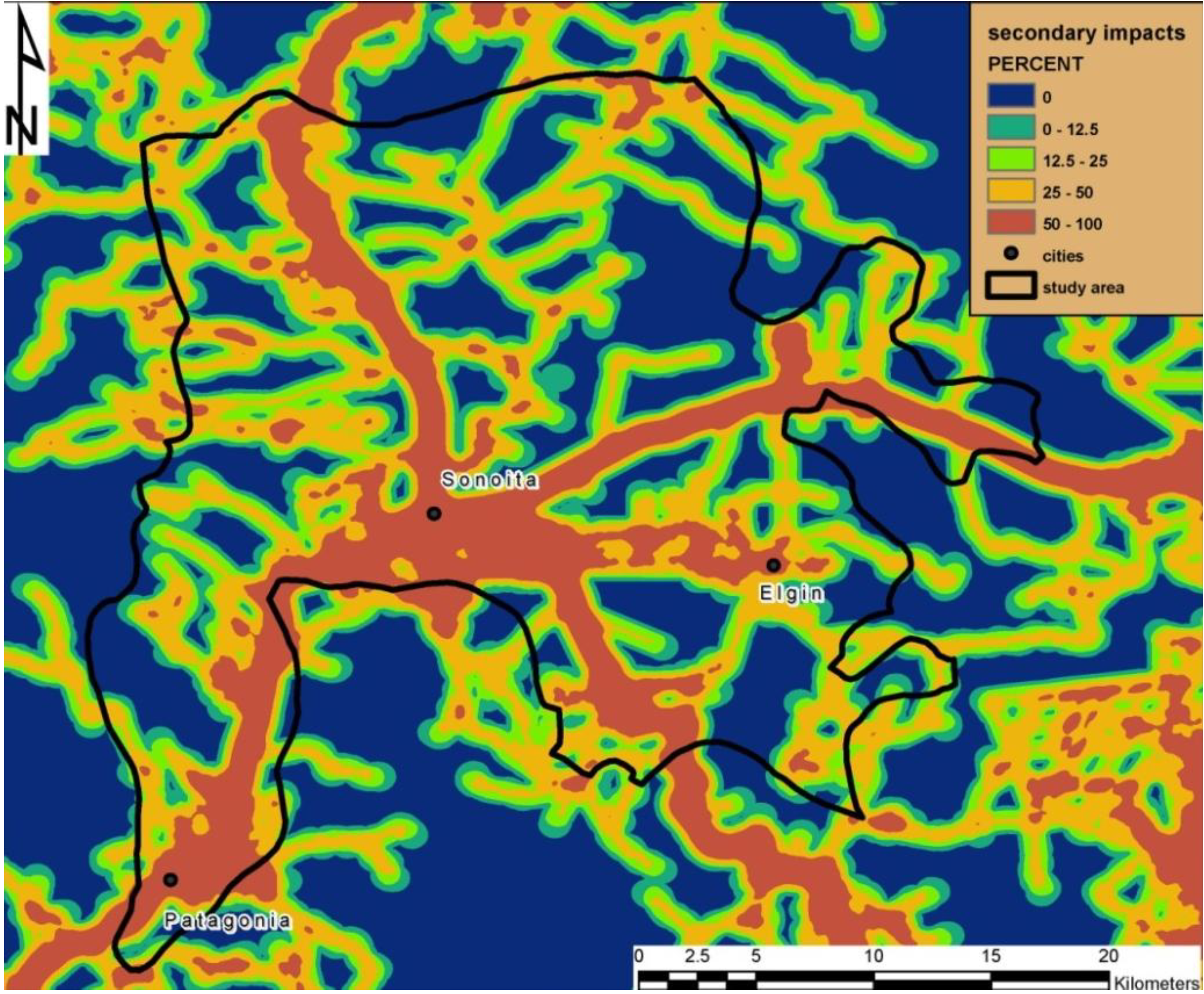
The cumulative impact of generalized distance effects provides a measure of the area surrounding each point that is affected by roads or houses. Cumulative impacts were determined by calculating the percentage of the landscape, within a 500-m radius circular neighborhood, that falls within a diffuse distance-effects zone (
Figure 4). In other words, in an area where there is a “High” impact from the cumulative effects of houses, 25%–50% of the area surrounding each point falls within 100 m of a house, 100 m of a road, or 500 m of a highway.
Figure 4.
Cumulative impacts of houses and roads on ecosystem function. The impacts represent the area within a 500-m circular neighborhood that lies within the impact zone of a house, road or highway.
Figure 4.
Cumulative impacts of houses and roads on ecosystem function. The impacts represent the area within a 500-m circular neighborhood that lies within the impact zone of a house, road or highway.
2. Results and Discussion
Within the study area, 1,867 houses were identified and mapped, which is equal to the number reported in the 2010 Census, and there were 943 km of roads. Both houses and roads are concentrated in and around the three towns in the study area (Sonoita, Elgin, and Patagonia). Following the housing density classes defined above, of the 69,519 ha study area, 91.5% (63,607 ha) is rural, 8.3% (5,762 ha) is exurban, and 0.2% (150 ha) is suburban.
2.1. Fire
Much of the study area has not been affected by fire for at least 25 years and fire potential presently appears to be a moderate to major threat to ecosystems and ecosystem function (
Table 3). Where they have occurred, recent fires in the Sonoita Plain mostly have been confined to bottomland areas, where stores of organic fuels have been relatively large, in areas of relatively high elevation with trees, and near towns where the fires may have been started by humans [
32]. The high FRID value in exurban areas suggests that fire suppression measures associated with exurban development have increased fire hazard in the area. Suburban areas have a more impervious surface, organic material tends to be cleared way, and there is a quick response to extinguish fires, and as such suburban areas have a much higher expected fire return interval (FRI) than exurban areas. Suburban (“Developed” according to the Southwest Regional Gap Analysis Program (SWReGap) [
18] classification) areas are expected to burn on average every 400+ years, while exurban areas (various “grassland” classes) naturally burn on average every 8–100 years.
Table 3.
Fire Return Departure (FRID) index values by housing-density class. Positive FRID values indicate fuel storage and moderate to high potential for fire, whereas negative numbers indicate a limited amount of fuel storage and low potential for fire.
Table 3.
Fire Return Departure (FRID) index values by housing-density class. Positive FRID values indicate fuel storage and moderate to high potential for fire, whereas negative numbers indicate a limited amount of fuel storage and low potential for fire.
| Housing-Density Class | Mean FRID | Area with Positive FRID (%) | Area with Negative FRID (%) | Mean Time Since Fire (years) |
|---|
| Study Area | 1.29 | 83.2 | 16.8 | 24.6 |
| Rural | 1.28 | 82.5 | 17.5 | 24.4 |
| Exurban | 1.47 | 92.7 | 7.3 | 26.4 |
| Suburban | −0.55 | 14.9 | 85.1 | 27.0 |
Even in rural areas, the quick response to extinguish fires means that much of the Sonoita Plain has not burned within normal fire-return intervals and that the build-up of organic fuels represents significant risk of large, high-intensity fires. The high FRID value in exurban areas may suggest that it is the presence of people rather than the density that increases fire hazard. This high fire hazard, combined with the large amount of land required to accommodate people at such low population densities, may challenge the perception of exurbanization as a conservation compatible land-use.
2.2. Water
The Sonoita Plain has experienced substantial change over the past 100 years due to increased ground water withdrawals for irrigation and domestic purposes [
33,
63] from a growing number of wells (
Table 4). Over the past 70 years, technological advances enabled deeper wells with increasingly powerful pumps [
33], and as water became a less limiting factor, more people settled in the Sonoita Plain. Wells are being dug deeper than in the past, suggesting a lowering of the water-table due to groundwater extraction (
Table 5). In addition to exurban development, this area, which was historically used for cattle ranching, has emerged as a viniculture center and is promoted as the wine capital of Arizona. The area is currently home to 10 vineyards. The period from 2000 to 2009 includes the largest housing boom in the region (2004–2006) and corresponds to the emergence of the three housing-density classes [
64].
Table 4.
Cumulative number of well in the study area, by decade (1970 through 2010).
Table 4.
Cumulative number of well in the study area, by decade (1970 through 2010).
| | Up to 1970 | Up to 1980 | Up to 1990 | Up to 2000 | Up to 2010 |
|---|
| Number of wells | 161 | 320 | 646 | 931 | 1,243 |
The number of wells in the study area was larger than expected. As of 2010, there were 1,243 wells for 1,867 households, which corresponds to 0.67 wells per household. When considered by housing-density class, there has been little increase in the number of new wells in suburban areas, with just three wells added in the last decade (
Table 5). Conversely, there has been a steady increase in the number of wells added in exurban areas (174 wells from 2000 to 2009). This growth is closely followed by the increase in the number of wells in rural areas (166 wells added from 2000 to 2009), which may be partly driven by the viniculture boom in the region. Depths to water were smallest in the most densely populated area, which likely reflects historic technological constraints and the siting of towns, as well as differences in underlying soil and bedrock [
32]. There is little difference in the depths to water between housing-density classes and the study area as a whole.
Table 5.
Average depth to water, by housing-density class, in 1970 and 2010. Many current houses were built after 1970 and housing densities were lower throughout the study area (i.e., exurban areas were likely rural in 1970), however the density classes were used to compare the effects of wells on ground water resources.
| | 2010 Depth (m) | 1970 Depth (m) | Difference in Depth 1970–2010 (m) | New Wells (2000–2009) |
|---|
| Study Area | 48.92 | 35.52 | 13.40 | 343 |
| Rural | 48.69 | 35.31 | 13.38 | 166 |
| Exurban | 52.18 | 38.57 | 13.61 | 174 |
| Suburban | 26.88 | 12.86 | 14.01 | 3 |
A recent study of water use in the Sonoita Plain revealed that residential developments and vineyards use significantly more water than do cattle ranches, where wells are widely spaced around the property to provide water for livestock [
65]. The study results estimate that the average annual recharge around the town of Sonoita (282 km
2 area) is 4.91 × 10
6 m
3 per year. Of this, 3.28 × 10
6 m
3 of water are accounted for, leaving approximately 1.62 × 10
6 m
3 available for future use. Under current zoning, that area could accommodate an additional 8,213 homes, withdrawing 4.82 × 10
6 m
3 of ground water annually. That withdrawal rate is three times greater than the surplus of water available for future development. Although annual recharge is not known for areas outside of the town of Sonoita, these rates are likely similar throughout the Sonoita Plain.
The detrimental effects of excessive ground water use are already evident in other communities in southeastern Arizona. Although the Sonoita Plain has not reached a critical point in its water use, the experiences of neighboring communities provide a sobering window into the future. Immediately northwest of the Sonoita Plain, the Tucson area (Pima County, AZ, USA) is experiencing ground water withdrawal-related land subsidence, in the form of sinks, on and near farmlands. The sinks occur in alluvial deposits along the flood plain of the Santa Cruz River and in some cases have made farmlands dangerous and unsuitable for farming; more than 1,700 sinks have been identified, which were likely caused by water-table decline and channel incision [
66]. Adjacent to the Sonoita Plain, flows of the Sand Pedro River, upon which the San Pedro National Riparian Conservation Area depends, are threatened by ground water withdrawals in the Sierra Vista area [
33].
A key ecosystem provision of grasslands is water for wildlife, and the water cycle controls this critical service. Important also is that the water balance of semiarid ecosystems can change dramatically in response to changing climate [
67,
68]. Recently, the Southwest has experienced pronounced drought that has reduced rates of stream flow and ground-water recharge, and has caused tree death in savannas owing to deficient soil moisture and increased vulnerability to insects. Research indicates that warming and drying in the Southwest will continue [
69]. The trends in water withdrawal and availability reported here may provide area residents with additional water management information, which in turn may help to avoid some of the problems experienced by other communities in the region.
2.3. Generalized Distance Effects of Houses and Roads
Although the generalized distance effects selected were conservative, about 35% of this sparsely populated landscape fell within the diffuse-effects zone of houses, roads, and highways (
Table 6). About 10% of the landscape fell within a concentrated-effects zone and has been intensely modified. The effects zones mainly followed the highways (State Routes 82 and 83) and areas with highest housing densities. Note that there is some overlap in the areas covered by roads and houses (e.g., roads lead to houses, so where they meet, the impact zones of houses and roads overlap).
Table 6.
Generalized distance effects of houses, roads and highways: (a) the areas impacted by the concentrated and diffuse effects of houses, roads, and highways; (b) the percentage area of each housing-density class impacted by distance effects; (c) the cumulative impacts of distance effects, by housing-density class.
| | |
| | Concentrated Effects (ha) | Study Area (%) | Diffuse Effects (ha) | Study Area (%) |
| Highways | 1,893 | 2.7 | 7,887 | 11.3 |
| Roads | 4,538 | 6.5 | 13,754 | 19.8 |
| Houses | 961 | 1.4 | 3,014 | 4.3 |
| (b) Effects Zones by Housing-Density Class (Concentrated and Diffuse Effects) |
| | House Effects Zones (% within Zone) | Road Effects Zones (% within Zone) | Highway Effects Zones (% within Zone) | All Effects Zones Combined (% within Zone) |
| Study Area | 4.3 | 19.8 | 11.4 | 28.5 |
| Rural | 1.4 | 16.1 | 9.8 | 24.2 |
| Exurban | 34.6 | 58.9 | 26.2 | 73.7 |
| Suburban | 90.7 | 95.8 | 85.7 | 99.6 |
| (c) Cumulative Impacts by Housing-Density Class |
| | Unaffected (0%) | Low (0%–12.5%) | Medium (12.5%−25%) | High (25%–50%) | Very High (50%–100%) |
| Study Area | 26.2 | 16.3 | 16.7 | 25.7 | 15.1 |
| Rural | 36.3 | 14.1 | 14.3 | 22.9 | 12.4 |
| Exurban | 0.0 | 0.2 | 1.8 | 17.3 | 80.7 |
| Suburban | 0.0 | 0.0 | 0.0 | 0.0 | 100.0 |
The cumulative impacts represent the area surrounding each point that is affected by roads and house, calculated as the percentage of area within a 500-m radius circular neighborhood that has concentrated or diffuse impacts from houses or roads (
Table 6). When the cumulative effects of these distance effects are considered, the impacts of dispersed housing, and its associated road networks are striking. An area was considered to be “Very Highly” impacted if 50%–100% of the 500-m circular neighborhood surrounding each point fell within a road, highway, or house-impact zone. Not surprisingly, 100% of the suburban density class was highly impacted. However, the percentage of area within the exurban density class that was also “Very Highly” impacted was 81%, which approaches that of areas with suburban densities. When both “Highly” impacted (25%–50% of the neighborhood lies within an effects zone) and “Very Highly” impacted areas were considered, 98% of exurban areas fell within these cumulative-effects categories. The cumulative effects of rural density classes were substantially lower, with only 12% of the area being “Very Highly” impacted.
Exurban areas support lower population densities than do suburban areas, but the associated houses and roads appear to have comparable impacts on ecological processes. Given the rapid growth of exurban housing throughout the United States, these impacts are potentially enormous. The results of this study support earlier work that found that development patterns that are more contiguous, higher density, and more compact have reduced overall effects on natural resources [
2]. The dispersed settlement patterns of exurban areas create practical complications for natural resource management and planning. The cumulative-effects method described here could be used as a rapid-assessment tool to compare alternative growth scenarios or for other planning applications. The specific parameters (effects zones, neighborhood size, impact categories,
etc.) can be easily modified, and this approach has the advantage of being spatially explicit.
Amenity-driven exurbanization is occurring across very different landscapes—from hobby farms in Oregon to the Florida everglades, in coastal communities in Australia, and at the forest-agriculture interface in Europe [
70]—which makes both the assessment of ecological impacts and comparisons across areas difficult. These are important land-use transitions and in order to scale up from case studies and to study exurbia at regional or national scales, we need to make the term operational. To effectively research, and then forecasting and plan, a better understanding of the impacts of exurbanization is necessary; a comparison of exurban areas to those with suburban and rural density classes serves to make discussions and comparisons of impacts operational. The three indictors of ecosystem function described here were used to assess the impacts of exurbanization in a semi-arid grassland, so additional metrics are likely necessary to study impacts in other systems. Assessment by housing-density class could serve as a template for cross-site comparative analysis of impacts in other regions, as this approach provides a flexible way to evaluate impact and compare regions. By focusing directly on the relationship between residential development and impacts, the approach described here could contribute to synthesis, scenario-planning, and the development of general theories of these relationships in space and time.
3. Conclusions
The impacts of exurban development seem disproportionate to the population densities that they support, and even at the lower population densities found in exurban areas, the effects on ecosystem function approach those found in suburban areas. This is especially true of the influence of exurban development on fire hazard and general distance effects on ecosystem function. When the per-capita impacts are considered, exurban development appears to present substantial risk to natural-resource sustainability. The findings here support earlier work on the ecological impacts of exurbanization [
2]. There is mounting evidence that, despite popular perception [
3,
15], exurbanization may not be a conservation compatible land-use. The comparisons between different housing density classes in this study were limited because there is only one suburban area (around the town of Patagonia) that was compared to multiple exurban and rural areas. The findings here may be a product of some particular characteristic(s) of the town of Patagonia rather than general suburban characteristics. It is difficult to find multiple occurrences of the three different housing classes within a constrained geographic area. Given current trends, it seems likely that within 20 years, housing densities in the towns of Sonoita and Elgin will reach suburban densities. A reassessment of trends at that time could be informative.
The impact of exurban development will depend on the ecosystem service considered, highlighting the challenge both of predicting and managing ecosystem function under changing land-use patterns. For example, in order to avoid mining of stored groundwater, which then remains available to carry the population through severe droughts and prevents damage to the ecosystem, a minimum lot size of 5 ha has been recommended [
65] around the town of Sonoita. While larger lot sizes, and therefore lower housing density, may be better for protecting water yield, if the rate of migration into the area continues and it is zoned at these lower housing densities, much more of the Sonoita Plain will be inhabited. This dispersed housing would likely result in many more kilometers of roads and their accompanying effects on ecological processes. Attempts to minimize impacts on water availability increase the impacts on other ecological processes through the production of road networks. The area described here is a healthy grassland ecosystem that is threatened by continuing development; nearby areas that have suffered ecosystem degradation provide comparisons and an ability to evaluate management approaches to avoid or mitigate further ecosystem compromise. To inform policy reliably, planning must consider a wide range of ecological processes or risk grave reductions of vital functions.
Grasslands provide many services, most of which currently have limited market value. Native grasslands contribute to maintaining the composition of the atmosphere by sequestering carbon, absorbing methane, and reducing emissions of nitrous oxide. Grasslands maintain a large genetic library, ameliorate regional climate, and preserve soil from erosion [
71]. The soils of these systems contain large quantities of carbon in their soils that is rapidly released into the atmosphere when plowed. However, the reverse process of accruing carbon is very slow [
72]. Similarly, native grasslands represent a reservoir of biological diversity, which is rapidly depleted after cultivation or overgrazing [
73]. Recovery is very slow, or may never occur, depending of the size of the disturbed area. Failure to value the services provided by grasslands has important consequences for decision-makers, researchers, and society. Assessing the spatial extent of threats to ecosystem services is an important step for understanding the vulnerability of the systems and guiding decisions on the fate and best use of grassland ecosystems.


