Land-Use Threats and Protected Areas: A Scenario-Based, Landscape Level Approach


Abstract
:
1. Introduction
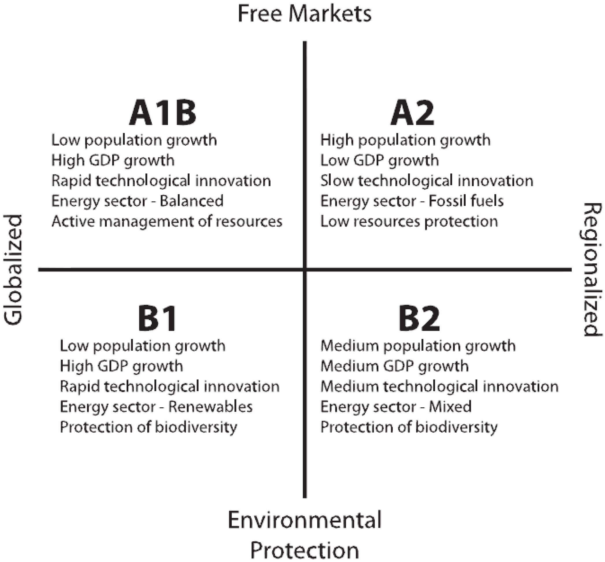
1.1. Land Use and Land Cover Scenarios

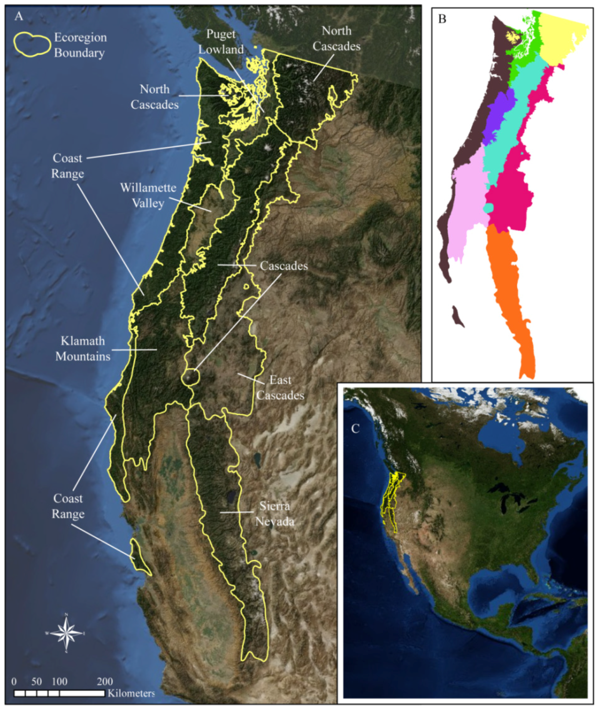
2. Study Region


3. Methods
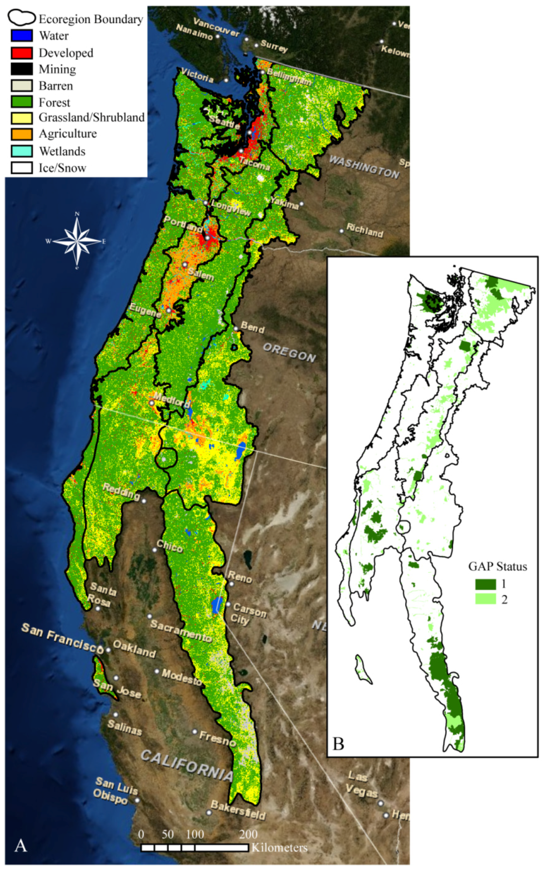
3.1. Protected Areas
3.2. State-and-Transition Modeling
3.3. Model Initiation

| Dataset | Date | Description | Reference |
|---|---|---|---|
| National Land Cover Dataset (NLCD) | 1992 20012006 | Land cover databases | [77] [78] [79] |
| NLCD Retro Product | 1992, 2001 | 1992–2001 retrofitted land cover change database | [80] |
| LANDFIRE’s Vegetation Change Tracker (VCT) | 1984–2010 | Annual forest disturbance | [81] |
| Web-enabled Landsat Data (WELD) | 2006–2011 | Forest declines over 5-year period | [82] |
| Cropland Data Layer (CDL) | 2010, 2011 | Crop specific estimates of crop acreage | [83] |
| Monitoring Trends in Burn Severity (MTBS) | 1984–2010 | Annual burn severity and wildfire perimeters | [84] |
| Forest Cover Types | 1991 | 25 classes of forest cover as well as water and non-forested lands | [85] |
3.4. Model Parameterization
| Spatial Multiplier | Description | Datasets and Reference |
|---|---|---|
| Forest Harvest | Sets parameters for allowable forest harvest transition based on distance to historic harvest (1984–2009 cumulative harvest from VCT), a majority filter of 8 pixels, and conversions on protected lands were restricted (GAP 1 & 2). | VCT [81] PAD-US [68] |
| Agriculture to Grassland/Shrubland | Sets probabilities of conversion based on distance to existing grassland/shrublands, low crop capability, a majority filter of 8 pixels, and restricts conversion on protected lands (GAP 1 & 2) | Harmonized LULC [75] Crop Capability [88] PAD-US [68] |
| To Developed | Sets probabilities of conversion into developed land with highest probability occurring on land closest to existing, high density development (>80 people/km2). Distance to development was calculated and pixels >20 km2 away from existing development were excluded. A majority filter of 8 pixels was also applied. Distance to development and distance to high population density were multiplied to produce final probability map. Conversions not allowed on protected lands (GAP Status 1 & 2) | Harmonized LULC [75] Population Density [89] PAD-US [68] |
| To Agriculture | Sets probabilities of conversion into agriculture based on distance to existing agriculture and crop capability. Restricts conversion on protected lands (GAP 1 & 2). | Harmonized LULC [75] PAD-US [68] |

3.5. Processing Model Output
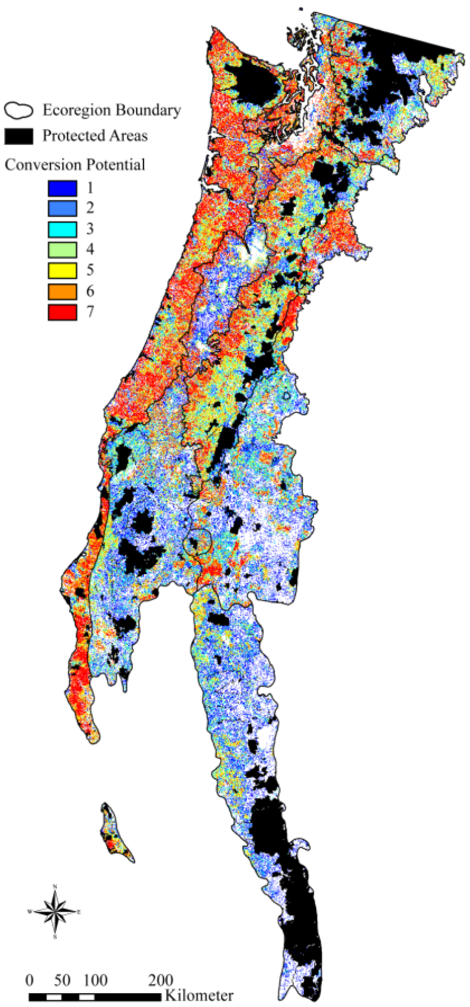
3.6. Land Conversion Potential and Conversion Threat Mapping

 is the projected land use and land cover (LULC) change in a cell for a given scenario (s1…n) for each year (y) over the modeled period. A value of 7 indicates all scenarios projected a change in LULC for that location, while a value of 0 indicates that none of the scenarios projected a change.
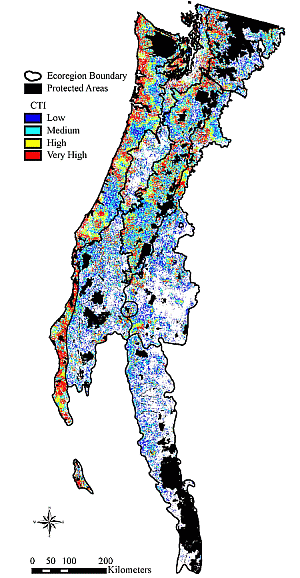
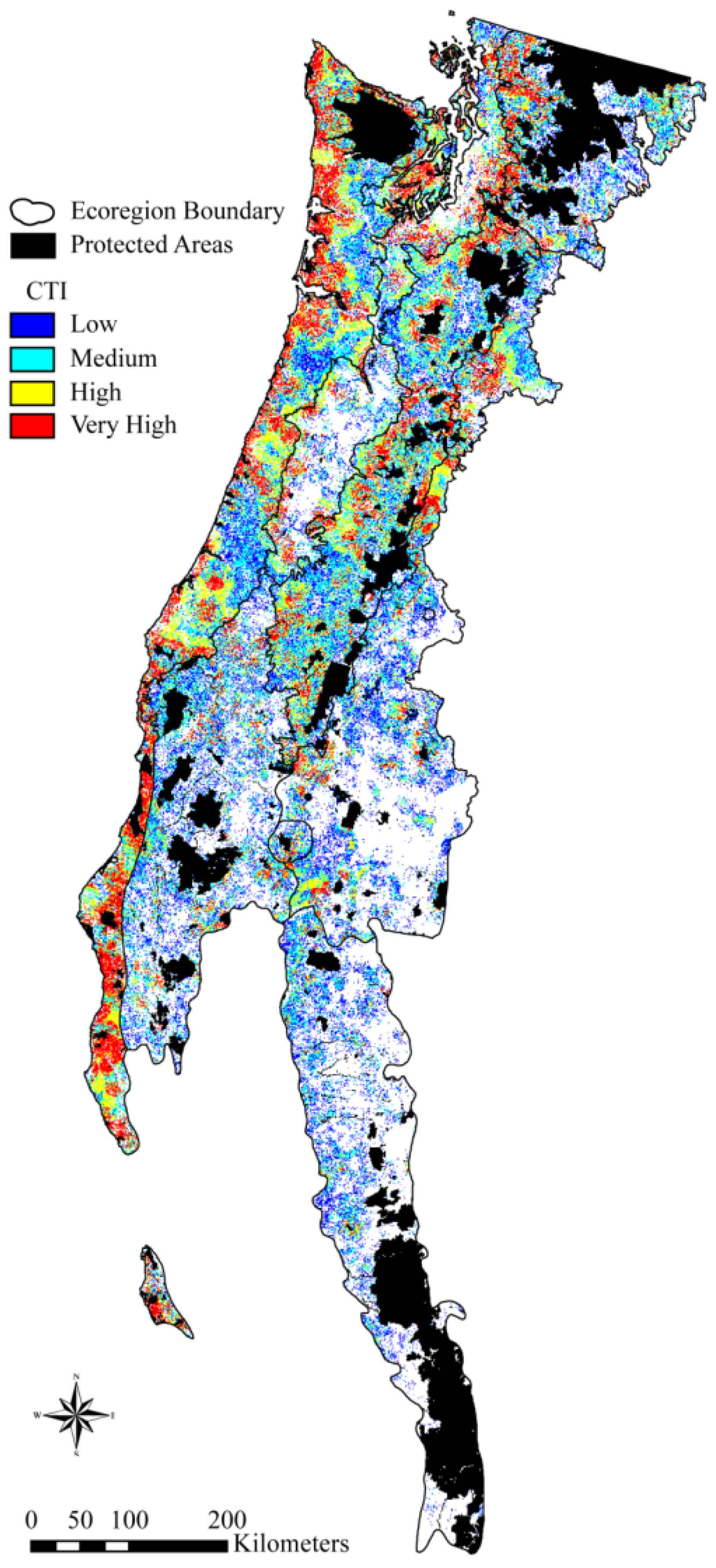
 represents the cell’s conversion potential over the model period and DTPA represents distance to protected area boundary. Resulting CTI values (from 1 to 35) were classified as follows: values 1–6, CTI = not classified (i.e., these values represent minimal scenario agreement at greater distances from a protected area boundary); values 7–12, CTI = low; values 13–20, CTI = medium; values 21–25, CTI = high; and values 26–35, CTI = very high. High CTI values correspond to the high conversion potential in closest proximity to protected areas.
4. Results
4.1. Changes in Development and Agricultural Land Use over the Modeled Period
| To Class | From Class | LULC Scenarios | ||||||
|---|---|---|---|---|---|---|---|---|
| A1B | A2 | B1 | B2 | Trends 86–92 | Trends 92–00 | Trends Random | ||
| Developed | Forest | 5745 | 8104 | 3360 | 2051 | 6600 | 6500 | 5565 |
| Agriculutre | 2810 | 3907 | 2086 | 1140 | 4412 | 2902 | 2900 | |
| Grassland/Shrubland | 950 | 978 | 943 | 741 | 800 | 900 | 760 | |
| All Other | 796 | 679 | 673 | 681 | 574 | 769 | 568 | |
| Total | 10,301 | 13,668 | 7062 | 4613 | 12,386 | 11,071 | 9793 | |
| Agriculture | Forest | 4800 | 9465 | 1171 | 1442 | 2494 | 900 | 1913 |
| Grassland/Shubland | 1831 | 1871 | 1395 | 1086 | 500 | 1199 | 904 | |
| Wetlands | 641 | 826 | 308 | 324 | 618 | 200 | 255 | |
| Total | 7272 | 12,162 | 2874 | 2852 | 3612 | 2299 | 3072 | |
| Developed and Agriculture | Total | 17,573 | 25,830 | 9936 | 7465 | 15,998 | 13,370 | 12,865 |
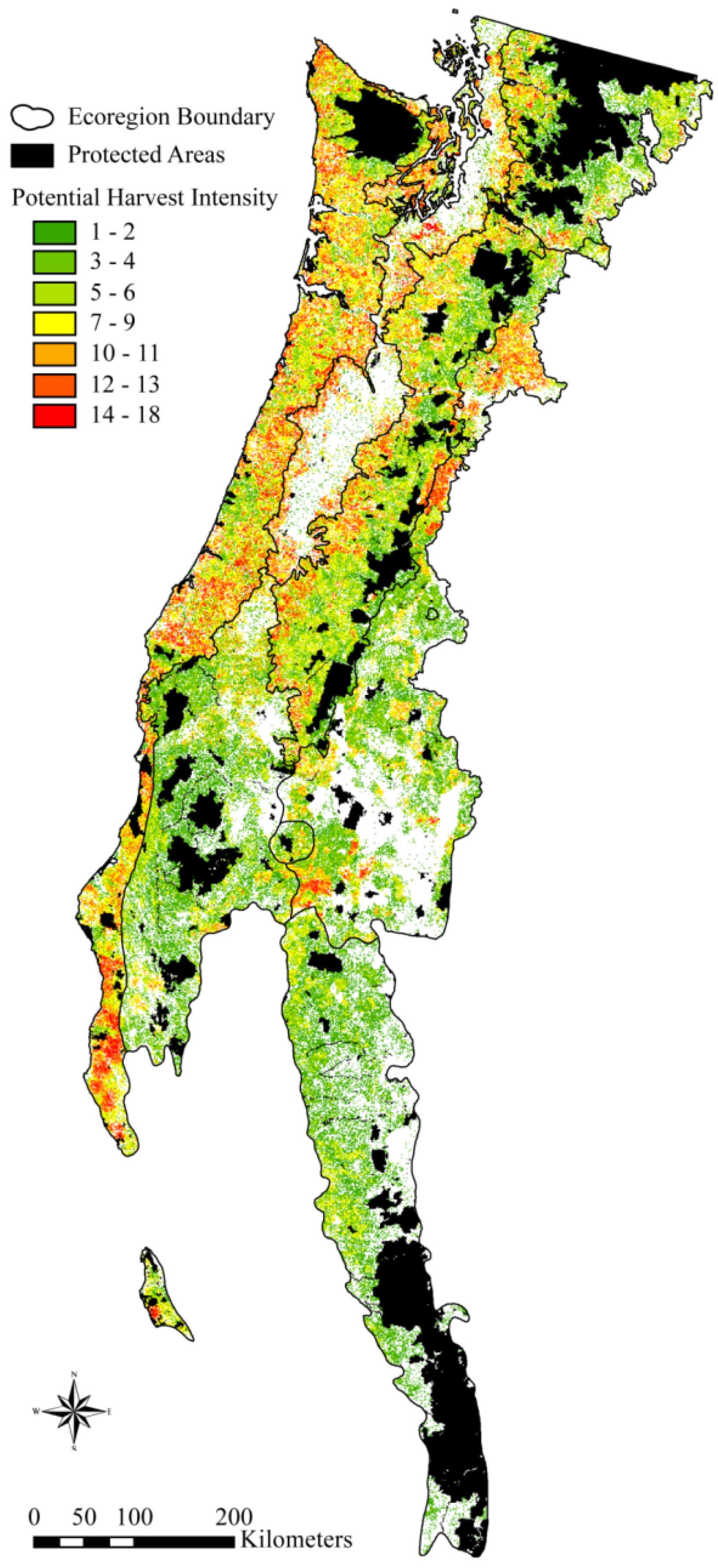
4.2. Forest Harvest
| LULC Scenarios | Forest Harvest Intensity | |||||||
|---|---|---|---|---|---|---|---|---|
| 1 | 2 | 3 | Total | |||||
| A1B | 66,972 | 21.0% | 57,931 | 18.1% | 2162 | 0.7% | 127,065 | 39.8% |
| A2 | 70,573 | 22.1% | 36,845 | 11.5% | 574 | 0.2% | 107,992 | 33.8% |
| B1 | 66,705 | 20.9% | 25,730 | 8.1% | 216 | 0.1% | 92,651 | 29.0% |
| B2 | 69,412 | 21.7% | 46,750 | 14.6% | 1304 | 0.4% | 117,466 | 36.8% |
| Trends 86–92 | 60,064 | 18.8% | 48,033 | 15.0% | 1714 | 0.5% | 109,811 | 34.4% |
| Trends 92–00 | 54,534 | 17.1% | 21,316 | 6.7% | 317 | 0.1% | 76,167 | 23.8% |
| Trends Random | 61,287 | 19.2% | 21,833 | 6.8% | 124 | 0.0% | 83,244 | 26.0% |

4.3. Conversion Potential

| Ecoregion | Conversion Potential | % Area in 7 | ||||||
|---|---|---|---|---|---|---|---|---|
| 1 | 2 | 3 | 4 | 5 | 6 | 7 | ||
| Coast Range | 2417 | 1390 | 2041 | 3342 | 5104 | 8386 | 17,132 | 31.7% |
| Puget Lowland | 1664 | 1110 | 656 | 599 | 1263 | 2729 | 3298 | 20.0% |
| Willamette Valley | 2875 | 1440 | 687 | 598 | 865 | 1292 | 1836 | 12.3% |
| Cascades | 2613 | 2722 | 3918 | 5082 | 5462 | 5873 | 5951 | 12.8% |
| Sierra Nevada | 6966 | 4083 | 2705 | 2083 | 1794 | 978 | 231 | 0.4% |
| East Cascades | 7244 | 4956 | 4765 | 4097 | 3413 | 3899 | 4699 | 8.4% |
| North Cascades | 2072 | 1787 | 1775 | 1927 | 1671 | 1367 | 1620 | 5.3% |
| Klamath Mountains | 6805 | 5375 | 4508 | 3594 | 3061 | 2507 | 1628 | 3.4% |
| TOTAL | 32,656 | 22,863 | 21,055 | 21,322 | 22,633 | 27,031 | 36,395 | 11.4% |
4.4. Protected Areas
| Ecoregion | Area (km2) | GAP 1 (km2) | GAP 2 (km2) | Total Protected (km2) | Total Protected (%) |
|---|---|---|---|---|---|
| Coast Range | 53,979 | 2799 | 2238 | 5037 | 9.3% |
| Puget Lowland | 16,456 | 29 | 301 | 330 | 2.0% |
| Willamette Valley | 14,874 | 0 | 186 | 186 | 1.2% |
| Cascades | 46,437 | 2196 | 7119 | 9315 | 20.1% |
| Sierra Nevada | 52,866 | 12,775 | 3179 | 15,954 | 30.2% |
| East Cascades | 56,115 | 283 | 2598 | 2881 | 5.1% |
| North Cascades | 30,312 | 3536 | 9618 | 13,154 | 43.4% |
| Klamath Mountains | 48,544 | 5127 | 2149 | 7276 | 15.0% |
| Total | 319,583 | 26,745 | 27,388 | 54,133 | 16.9% |
4.5. Conversion Threat Index
| CTI Value | ||||||||
|---|---|---|---|---|---|---|---|---|
| Low | Medium | High | Very High | |||||
| Coast Range | 5230 | 9.7% | 10,385 | 19.2% | 9264 | 17.2% | 11,728 | 21.7% |
| Puget Lowland | 1697 | 10.3% | 2605 | 15.8% | 2267 | 13.8% | 2676 | 16.3% |
| Willamette Valley | 1743 | 11.7% | 1918 | 12.9% | 1273 | 8.6% | 888 | 6.0% |
| Cascades | 5963 | 12.8% | 11,118 | 23.9% | 6058 | 13.0% | 5083 | 10.9% |
| Sierra Nevada | 5893 | 11.1% | 3529 | 6.7% | 674 | 1.3% | 302 | 0.6% |
| East Cascades | 8380 | 14.9% | 7609 | 13.6% | 3731 | 6.6% | 2787 | 5.0% |
| North Cascades | 2784 | 9.2% | 3542 | 11.7% | 1604 | 5.3% | 1966 | 6.5% |
| Klamath Mountains | 7785 | 16.0% | 7279 | 15.0% | 2330 | 4.8% | 1651 | 3.4% |
| Total | 39,475 | 12.4% | 47,985 | 15.0% | 27,201 | 8.5% | 27,081 | 8.5% |

5. Discussion
6. Conclusions
Acknowledgments
Authors Contributions
Conflicts of Interest
Disclaimer
References
- Dale, V.H. The relationship between land-use change and climate change. Ecol. Appl. 1997, 7, 753–769. [Google Scholar] [CrossRef]
- Turner, B.L., II; Clark, W.C.; Kates, R.M.; Richards, J.F.; Mathews, J.T.; Meyer, M.B. (Eds.) The Earth as Transformed by Human Action: Global and Regional Changes in the Biosphere over the Past 300 Years; Cambridge University Press: Cambridge, UK, 1990; p. 713.
- Vitousek, P.M.; Mooney, H.A.; Lubchenco, J.; Melillo, J.M. Human domination of earth’s ecosystems. Science 1997, 277, 494–499. [Google Scholar] [CrossRef]
- Sala, O.E.; Chapin, F.S.; Armesto, J.J.; Berlow, E.; Bloomfield, J.; Dirzo, R.; Huber-Sanwald, E.; Huenneke, L.F.; Jackson, R.B.; Kinzig, A.; et al. Global biodiversity scenarios for the year 2100. Science 2000, 287, 1770–1774. [Google Scholar] [CrossRef]
- Soule, M.E. Conservation: Tactics for a constant crisis. Science 2001, 253, 744–750. [Google Scholar]
- Seabloom, E.W.; Dobson, A.P.; Stoms, D.M. Extinction rates under nonrandom patterns of habitat loss. Proc. Natl. Acade. Sci. USA 2002, 99, 11229–11234. [Google Scholar] [CrossRef]
- Swaty, R.; Blankenship, K.; Hagen, S.; Fargione, J.; Smith, J.; Patton, J. Accounting for ecosystem alteration doubles estimates of conservation risk in the conterminous United States. PLoS One 2011, 6, e23002. [Google Scholar]
- Davies, R.G.; Orme, D.L.; Olson, V.; Thomas, G.H.; Ross, S.G.; Ding, T.-S.; Rasmussen, P.C.; Stattersfield, A.J.; Bennett, P.M.; Blackburn, T.M.; et al. Human impacts and the global distribution of extinction risk. Proc. R. Soc. Biol. Sci. 2006, 273, 2127–2133. [Google Scholar] [CrossRef]
- Rittenhouse, C.D.; Pidgeon, A.M.; Albright, T.P.; Culbert, P.D.; Clayton, M.K.; Flather, C.H.; Masek, J.G.; Radeloff, V.C. Land-cover change and avian diversity in the conterminous United States. Conserv. Biol. 2012, 26, 821–829. [Google Scholar] [CrossRef]
- Foley, J.A.; DeFries, R.; Asner, G.P.; Barford, C.; Bonan, G.; Carpenter, S.R.; Chapin, F.S.; Coe, M.T.; Daily, G.C.; Gibbs, H.K.; et al. Global consequences of land use. Science 2005, 309, 570–574. [Google Scholar] [CrossRef]
- Romero, H.; Ihl, M.; Rivera, A.; Zalazar, P.; Azocar, P. Rapid urban growth, land-use changes and air pollution in Santiago, Chile. Atmos. Environ. 1999, 33, 4039–4047. [Google Scholar] [CrossRef]
- Ross, Z.; English, P.B.; Scalf, R.; Gunier, R.; Smorodinsky, S.; Wall, S.; Jerrett, M. Nitrogen dioxide prediction in southern California use land use regression modeling: Potential for environmental health analyses. J. Expos. Sci. Environ. Epidemiol. 2006, 16, 106–114. [Google Scholar] [CrossRef]
- Houghton, R.A.; Hackler, J.L. Carbon Flux to the Atmosphere from Land-Use Changes: 1850 to 1990; ORNL/CDIAC-131, NDP-050/R1; Carbon Dioxide Information Analysis Center, U.S. Department of Energy, Oak Ridge National Laboratory: Oak Ridge, TN, USA, 2001; p. 18. [Google Scholar]
- Bonan, G.B. Effects of land use on the climate of the United States. Clim. Chang. 1997, 37, 449–486. [Google Scholar] [CrossRef]
- Pielke, R.A.; Marland, G.; Betts, R.A.; Chase, T.N.; Eastman, J.L.; Niles, J.O.; Niyogi, D.D.S.; Running, S.W. The influence of land-use change and landscape dynamics on the climate system: Relevance to climate-change policy beyond the radiative effect of greenhouse gases. Philos. Trans. R. Soc. Lond. 2002, 360, 1705–1719. [Google Scholar] [CrossRef]
- Lawrence, P.L.; Chase, T.N. Investigating the climate impacts of global land cover change in the community climate system model. Int. J. Clim. 2010, 30, 2066–2087. [Google Scholar] [CrossRef]
- Pitman, A.J.; Avila, F.B.; Abramowitz, G.; Wang, Y.P.; Phipps, S.J.; de Noblet-Ducoudre, N. Importance of background climate in determining the impact of land-cover change on regional climate. Nat. Clim. Chang. 2011, 1, 472–475. [Google Scholar] [CrossRef]
- Fischer, J.; Lindenmayer, D.B. Landscape modification and habitat fragmentation: A synthesis. Glob. Ecol. Biogeogr. 2007, 16, 265–280. [Google Scholar] [CrossRef]
- Sleeter, B.M.; Wilson, T.S.; Acevedo, W. (Eds.) Status and Trends of Land Change in the Western United States–1973 to 2000; Geological Survey Professional Paper 1794-A; U.S. Geological Survey: Reston, VA, USA, 2012; p. 324.
- Primack, R.B. Essentials of Conservation Biology, 5th ed.; Sinauer Associates, Inc.: Sunderland, MA, USA, 2010; p. 601. [Google Scholar]
- Cole, D.N.; Landres, P.B. Threats to wilderness ecosystems: Impacts and research needs. Ecol. Appl. 1996, 6, 168–184. [Google Scholar] [CrossRef]
- Hansen, A.J.; DeFries, R. Ecological mechanisms linking protected areas to surrounding lands. Ecol. Appl. 2007, 17, 974–988. [Google Scholar] [CrossRef]
- Hansen, A.J.; Rasker, R.; Maxwell, B.; Rotella, J.J.; Johnson, J.D.; Parmenter, A.W.; Langner, U.; Cohen, W.B.; Lawrence, R.L.; Kraska, M.P.V. Ecological causes and consequences of demographic change in the New West. BioScience 2002, 52, 151–162. [Google Scholar] [CrossRef]
- Joppa, L.N.; Loarie, S.R.; Pimm, S.L. On the protection of “protected areas.”. Proc. Natl. Acad. Sci. USA 2008, 105, 6673–6678. [Google Scholar] [CrossRef]
- Radeloff, V.C.; Nelson, E.; Plantinga, A.J.; Lewis, D.J.; Helmers, D.; Lawler, J.J.; Withey, J.C.; Beaudry, F.; Martinuzzi, S.; Butsic, V.; et al. Economic-based projections of future land use in the conterminous United States under alternative policy scenarios. Ecol. Appl. 2012, 22, 1036–1049. [Google Scholar] [CrossRef]
- Hamilton, C.M.; Martinuzzi, S.; Plantinga, A.J.; Radeloff, V.C.; Lewis, D.J.; Thogmartin, W.E.; Heglund, P.J.; Pidgeon, A.M. Current and future land use around a nationwide protected area network. PLoS One 2013, 8, e55737. [Google Scholar] [CrossRef] [Green Version]
- Wade, A.A.; Theobald, D.M. Residential development encroachment on U.S. protected areas. Conserv. Biol. 2010, 24, 151–161. [Google Scholar] [CrossRef]
- Pitelka, L.F. Plant migration and climate change: A more realistic portrait of plant migration is essential to predicting biological responses to global warming in a world drastically altered by human activity. Am. Sci. 1997, 85, 464–473. [Google Scholar]
- Ritters, K.H.; Wickham, J.D. How far to the nearest road? Front. Ecol. Environ. 2003, 1, 125–129. [Google Scholar] [CrossRef]
- Radeloff, V.C.; Stewart, S.I.; Hawbaker, T.J.; Gimmi, U.; Pidgeon, A.M.; Flather, C.H.; Hammer, R.B.; Helmers, D.P. Housing growth in and near United States protected areas limits their conservation value. Proc. Natl. Acad. Sci. USA 2010, 107, 940–945. [Google Scholar] [CrossRef]
- Nagenda, H. Do parks work? Impact of protected areas on land cover clearing. AMBIO 2008, 37, 330–337. [Google Scholar] [CrossRef]
- McLaughlin, A.; Mineau, P. The impact of agricultural practices on biodiversity. Agric. Ecosyst. Environ. 1995, 55, 201–212. [Google Scholar] [CrossRef]
- Neary, D.G.; Hornbeck, J.W. Impacts of harvesting and associated practices on off-site environmental quality. In Impacts of Forest Harvesting on Long-Term Site Productivity, 1st ed.; Dyck, W.J., Cole, D.W., Comerford, N.B., Eds.; Chapman and Hall: Suffolk, VA, USA, 1994; pp. 81–118. [Google Scholar]
- Nave, L.E.; Vance, E.D.; Swanston, C.W.; Curtis, P.S. Harvest impacts on soil carbon storage in temperate forests. For. Ecol. Manag. 2010, 259, 857–866. [Google Scholar] [CrossRef]
- Ricketts, T.; Imhoff, M. Biodiversity, urban areas, and agriculture: Locating priority ecoregions for conservation. Conserv. Biol. 2003, 8, 1. [Google Scholar]
- Wilson, K.; Pressey, R.L.; Newton, A.; Burgman, M.; Possingham, H.; Weston, C. Measuring and incorporating vulnerability into conservation planning. Environ. Manag. 2005, 35, 527–543. [Google Scholar] [CrossRef]
- McDonald, R.I.; Yuan-Farrell, C.; Fievet, C.; Moeller, M.; Kareiva, P.; Foster, D.; Gragson, T.; Kinzig, A.; Kuby, L.; Redman, C. Estimating the effect of protected lands on the development and conservation of their surroundings. Conserv. Biol. 2007, 21, 1526–1536. [Google Scholar]
- Wilson, T.S.; Sleeter, B.M.; Davis, A.W. Projected future land use threats to California’s protected areas. Reg. Environ. Chang. 2014. under review. [Google Scholar]
- Gude, P.H.; Hansen, A.J.; Jones, D.A. Biodiversity consequences of alternative future land use scenarios in greater Yellowstone. Ecol. Appl. 2007, 17, 1004–1018. [Google Scholar] [CrossRef]
- Margules, C.R.; Pressey, R.L. Systematic conservation planning. Nature 2000, 405, 243–253. [Google Scholar] [CrossRef]
- Defries, R.; Hansen, A.; Turner, B.L.; Reid, R.; Liu, J. Land use change around protected areas: Management to balance human needs and ecological function. Ecol. Appl. 2007, 17, 1031–1038. [Google Scholar] [CrossRef]
- Newburn, D.; Reed, S.; Berck, P.; Merenlender, A. Economics and land-use change in prioritizing private land conservation. Conserv. Biol. 2005, 19, 1411–1420. [Google Scholar] [CrossRef]
- IPCC Special Report on Emission Scenarios; Nakicenovic, N.; Swart, R. (Eds.) Cambridge University Press: Cambridge, UK; p. 570.
- Heistermann, M.; Müller, C.; Ronneberger, K. Land in sight? Achievements, deficits, and potentials of continental to global scale land-use modeling. Agric. Ecosyst. Environ. 2006, 114, 141–158. [Google Scholar] [CrossRef]
- Rounsevell, M.D.A.; Reginster, I.; Araújo, M.B.; Carter, T.R.; Dendoncker, N.; Ewert, F.; House, J.I.; Kankaanpää, S.; Leemans, R.; Metzger, M.J.; et al. A coherent set of future land use change scenarios for Europe. Agric. Ecosyst. Environ. 2006, 114, 57–68. [Google Scholar] [CrossRef]
- Alcamo, J.; Kok, K.; Busch, G.; Priess, J. Searching for the future of land: Scenarios from the local to global scale. In Environmental Futures: The Practice of Environmental Scenario Analysis; Alcamo, J., Ed.; Elsevier: Amsterdam, The Netherlands, 2008; pp. 67–103. [Google Scholar]
- Luoto, M.; Virkkala, R.; Heikkinen, R.K. The role of land cover in bioclimatic models depends on spatial resolution. Glob. Ecol. Biogeogr. 2007, 16, 34–42. [Google Scholar] [CrossRef]
- Strayer, D.L.; Beighley, R.E.; Thompson, L.C.; Brooks, S.; Nilsson, C.; Pinay, G.; Naiman, R.J. Effects of land cover on stream ecosystems: Roles of empirical models and scaling issues. Ecosytems 2003, 6, 407–423. [Google Scholar] [CrossRef]
- Zhao, S.; Liu, S.; Sohl, T.; Young, C.; Werner, J. Land use and carbon dynamics in the southeastern United States from 1992 to 2050. Environ. Res. Lett. 2013, 8, 044022:9. [Google Scholar]
- Sohl, T.L.; Sayler, K.L.; Bouchard, M.A.; Reker, R.R.; Friesz, A.M.; Bennett, S.L.; Sleeter, B.M.; Sleeter, R.R.; Wilson, T.S.; Knuppe, M.; et al. Spatially explicit modeling of 1992 to 2100 land cover and forest stand age for the conterminous United States. Ecol. Appl. 2013. [Google Scholar] [CrossRef]
- Wear, D.N. Forecasts of County-Level Land Uses Under Three Future Scenarios: A Technical Document Supporting the Forest Service 2010 RPA Assessment; Gen. Tech. Rep. SRS-141; U.S. Department of Agriculture Forest Service, Southern Research Station: Asheville, NC, USA, 2011; p. 41. [Google Scholar]
- Zhu, Z. (Ed.) Baseline and Projected Future Carbon Storage and Greenhouse-Gas Fluxes in the Great Plains Region of the United States; U.S. Geological Survey Professional Paper 1787; U.S. Geological Survey: Reston, VA, USA, 2011; p. 28.
- Sleeter, B.M.; Sohl, T.L.; Wilson, T.S.; Sleeter, R.R.; Soulard, C.E.; Bouchard, M.A.; Sayler, K.L.; Reker, R.R.; Griffith, G.E. Projected land-use and land-cover change in the Western United States. In Baseline and Projected Future Carbon Storage and Greenhouse-Gas Fluxes in Ecosystems of the Western United States; U.S. Geological Survey Professional Paper 1797A; Zhu, Z., Reed, B.C., Eds.; U.S. Geological Survey: Reston, VA, USA, 2012; pp. 65–86. [Google Scholar]
- Sohl, T.L.; Sleeter, B.M.; Sayler, K.L.; Bouchard, M.A.; Reker, R.R.; Bennett, S.L.; Sleeter, R.R.; Kanengieter, R.L.; Zhu, Z. Spatially explicit land-use and land-cover scenarios for the Great Plains of the United States. Agric. Ecosyst. Environ. 2012, 153, 1–15. [Google Scholar] [CrossRef]
- Wilson, T.S.; Sleeter, B.S.; Sohl, T.L.; Griffith, G.; Acevedo, W.; Bennett, S.; Bouchard, M.; Reker, R.; Ryan, C.; Sayler, K.L.; et al. Future Scenarios of Land-Use and Land-Cover Change in the United States: The Marine West Coast Forests Ecoregion; U.S. Geological Survey Open File Report 2012–1252; U.S. Geological Survey: Reston, VA, USA, 2012; p. 14. [Google Scholar]
- Arnell, N.W.; Livermore, M.J.L.; Kovats, S.; Levy, P. Climate and socioeconomic scenarios for global-scale climate change impacts assessments: Characterizing the SRES storylines. Glob. Environ. Chang. 2004, 14, 3–20. [Google Scholar] [CrossRef]
- Gaffin, S.R.; Rosenzweig, C.; Xing, X.; Yetman, G. Downscaling and geo-spatial gridding of socio-economic projections from the IPCC Special Report on Emissions Scenarios (SRES). Glob. Environ. Chang. 2004, 14, 105–123. [Google Scholar] [CrossRef]
- Verburg, P.H.; Schulp, C.J.E.; Witte, N.; Veldkamp, A. Downscaling of land use change scenarios to assess the dynamics of European landscapes. Agric. Ecosyst. Environ. 2006, 114, 39–56. [Google Scholar] [CrossRef]
- Van Vuuren, D.P.; Lucas, P.L.; Hilderink, H. Downscaling drivers of global environmental change scenarios: Enabling use of the IPCC-SRES scenarios at the national and grid level. Glob. Environ. Chang. 2007, 17, 114–130. [Google Scholar] [CrossRef]
- Sleeter, B.M.; Sohl, T.L.; Bouchard, M.A.; Reker, R.R.; Soulard, C.E.; Acevedo, W.; Griffith, G.E.; Sleeter, R.R.; Auch, R.F.; Sayler, K.L.; et al. Scenarios of land use and land cover change in the conterminous Unites States: Utilizing the special report on emission scenarios at ecoregional scales. Glob. Environ. Chang. 2012, 22, 896–914. [Google Scholar] [CrossRef]
- Sleeter, B.M.; Sohl, T.L.; Loveland, T.R.; Auch, R.F.; Acevedo, W.; Drummond, M.A.; Sayler, K.L.; Stehman, S.V. Land-cover change in the conterminous United States from 1973–2000. Glob. Environ. Chang. 2013, 23, 733–748. [Google Scholar] [CrossRef]
- U.S. Environmental Protection Agency. Level III Ecoregions of the Continental United States, Digital map, scale 1:250,000; U.S. Environmental Protection Agency, National Health and Environmental Effects Research Laboratory: Corvallis, OR, USA, 2013. Available online: ftp://ftp.epa.gov/wed/ecoregions/us/us_eco_l3.zip (accessed on 1 April 2014).
- Sleeter, B.M.; Soulard, C.E.; Wilson, T.S.; Sorenson, D.G. Land-cover trends in the Western United States—1973 to 2000. In Status and Trends of Land Change in the Western United States—1973 to 2000; Professional Paper 1794-A; Sleeter, B.M., Wilson, T.S., Acevedo, W., Eds.; Geological Survey: Reston, VA, USA, 2012; pp. 3–29. [Google Scholar]
- Omernik, J.M. Ecoregions of the conterminous United States. Ann. Assoc. Am. Geogr. 1987, 77, 118–125. [Google Scholar] [CrossRef]
- Gallant, A.L.; Loveland, T.R.; Sohl, T.L.; Napton, D. Using a geographic framework for analyzing land cover issues. Environ. Manag. 2004, 34, 89–110. [Google Scholar] [CrossRef]
- Herger, L.G.; Weiss, A.; Augustine, S.; Hayslip, G. Modeling Fish Distributions in the Pacific Northwest Coast Range Ecoregion Using EMAP Data; U.S. Environmental Protection Agency: Seattle, WA, USA, 2003; pp. 1–48. [Google Scholar]
- Mote, P.W.; Parson, E.A.; Hamlet, A.F.; Keeton, W.S.; Lettenmaier, D.; Mantua, N.; Miles, E.L.; Peterson, D.W.; Peterson, D.L.; Slaughter, R.; et al. Preparing for climatic change: The water, salmon, and forests of the Pacific Northwest. Clim. Chang. 2003, 61, 45–88. [Google Scholar] [CrossRef]
- U.S. Geological Survey GAP. Protected Areas Database of the United States (PAD-US), version 1.3 Combined Feature Class. 2012. Available online: http://gapanalysis.usgs.gov/padus/ (accessed on 13 November 2013). [Google Scholar]
- Kerns, B.K.; Shlisky, A.J.; Daniel, C.J. Proceedings of the First Landscape State-and-Transition Simulation Modeling Conference, Portland, OR, USA, 14–16 June 2011; General Technical Report PNW-GTR-869. U.S. Department of Agriculture, Forest Service, Pacific Northwest Research Station: Portland, OR, USA, 2012; p. 215.
- Daniel, C.J.; Frid, L. Predicting landscape vegetation dynamics using state-and-transition simulation models. In Proceedings of the First Landscape State-and-Transition Simulation Modeling Conference, Portland, OR, USA, 14–16 June 2011; Kerns, B.K., Shlisky, A.J., Daniel, C.J., Eds.; U.S. Department of Agriculture, Forest Service, Pacific Northwest Research Station: Portland, OR, USA, 2012; pp. 5–22. [Google Scholar]
- Shlisky, A.J.; Vandendriesche, D. Use of state-and-transition modeling in National Forest planning in the Pacific Northwest, USA. In Proceedings of the First Landscape State-and-Transition Simulation Modeling Conference, Portland, OR, USA, 14–16 June 2011; Kerns, B.K., Shlisky, A.J., Daniel, C.J., Eds.; U.S. Department of Agriculture, Forest Service, Pacific Northwest Research Station: Portland, OR, USA, 2012; pp. 23–42. [Google Scholar]
- Publications Using State-and-Transition Simulation Models. Available online: http://wiki.syncrosim.com/index.php?title=Publications (accessed on 25 November 2013).
- Steele, C.M.; Bestelmeyer, B.T.; Burkett, L.M.; Smith, P.L.; Yanoff, S. Spatially explicit representation of state-and-transition models. Rangeland Ecol. Manag. 2012, 65, 213–222. [Google Scholar] [CrossRef]
- State-and-Transition Simulation Models, APEX Resource Management Solutions, Ottawa, ON, Canada. Available online: http://www.apexrms.com/projects/stsm (accessed on 10 November 2013).
- Soulard, C.E.; Acevedo, W. Multi-temporal harmonization of independent land-use/land-cover datasets for the conterminous United States. In Proceedings of the Presentation at the American Geophysical Union, San Francisco, CA, USA, 9–13 December 2013.
- Anderson, J.R.; Hardy, E.E.; Roach, J.T.; Witmer, R.E. A Land Use and Land Cover Classification Scheme for Use with Remote Sensor Data; Professional Paper 964; U.S. Geological Survey: Reston, VA, USA, 1976; p. 28. [Google Scholar]
- Vogelmann, J.E.; Howard, S.M.; Yang, L.; Larson, C.R.; Wylie, B.K.; van Driel, J.N. Completion of the 1990’s national land cover data set for the conterminous United States. Photogramm. Eng. Remote Sens. 2001, 67, 650–662. [Google Scholar]
- Homer, C.; Dewitz, J.; Fry, J.; Coan, M.; Hossain, N.; Larson, C.; Herold, N.; McKerrow, A.; VanDriel, J.N.; Wickham, J. Completion of the 2001 national land cover database for the conterminous United States. Photogramm. Eng. Remote Sens. 2007, 73, 337–341. [Google Scholar]
- Fry, J.; Xian, G.; Jin, S.; Dewitz, J.; Homer, C.; Yang, L.; Barnes, C.; Herold, N.; Wickham, J. Completion of the 2006 national land cover database for the conterminous United States. Photogramm. Eng. Remote Sens. 2011, 77, 858–864. [Google Scholar]
- Fry, J.A.; Coan, M.J.; Homer, C.G.; Meyer, D.K.; Wickham, J.D. Completion of the National Land Cover Database (NLCD) 1992–2001 Land Cover Change Retrofit Product; Open-File Report 2008–1379; U.S. Geological Survey: Reston, VA, USA, 2009; p. 18. [Google Scholar]
- Huang, C.; Goward, S.N.; Masek, J.G.; Thomas, N.; Zhu, Z.; Vogelmann, J.E. An automated approach for reconstructing recent forest disturbance history using dense Landsat time series stacks. Remote Sens. Environ. 2010, 114, 183–198. [Google Scholar] [CrossRef]
- Roy, D.P.; Ju, J.; Kline, K.; Scaramuzza, P.L.; Kovalskyy, V.; Hansen, M.C.; Loveland, T.R.; Vermote, E.F.; Zhang, C. Web-enabled Landsat data (WELD): Landsat ETM+ composited mosaics of the conterminous United States. Remote Sens. Environ. 2010, 114, 35–49. [Google Scholar] [CrossRef]
- U.S. Department of Agriculture, National Agricultural Statistics Service (NASS). Cropland Data Layer for the United States; U.S. Department of Agriculture: Washington, DC, USA, 2011. [Google Scholar]
- Eidenshink, J.; Schwind, B.; Brewer, K.; Zhu, Z.; Quayle, B.; Howard, S. A project for monitoring trends in burn severity. Fire Ecol. Spec. Issue 2007, 3, 3–21. [Google Scholar]
- U.S. Department of Agriculture, Forest Service, U.S. Geological Survey. Forest Cover Types: National Atlas of the United States, Reston, VA, USA, 2002. Available online: http://nationalatlas.gov/metadata/foresti020l.faq.html (accessed on 15 December 2013).
- Villareal, M.L.; van Riper, C.; Petrakis, R.E. Conflation and aggregation of spatial data improve predictive models for species with limited habitats: A case of the threatened yellow-billed cuckoo in Arizona, USA. Appl. Geogr. 2014, 47, 57–69. [Google Scholar] [CrossRef]
- Pan, Y.; Chen, J.M.; Birdsey, R.; McCullough, K.; He, L.; Deng, F. Age structure and disturbance legacy of North American forests. Biogeosciences 2011, 8, 715–732. [Google Scholar] [CrossRef]
- Natural Resources Conservation Service. Soil Survey Geographic (SSURGO) Database; U.S. Department of Agriculture, 2011. Available online: http://soildatamart.nrcs.usda.gov (accessed on 22 November 2013).
- Sleeter, R.; Gould, M. Geographic Information System Software to Remodel Population Data Using Dasymetric Mapping Methods; U.S. Geological Survey Techniques and Methods 11-C2; U.S. Geological Survey: Reston, VA, USA, 2007; p. 15. [Google Scholar]
- Beaumont, L.J.; Duursma, D. Global projections of 21st century land-use changes in regions adjacent to protected areas. PLoS One 2012, 7, e43714. [Google Scholar] [CrossRef]
- Daniels, J.M. The Rise and Fall of the Pacific Northwest Log Export Market; General Technical Report, PNW-GTR-624; U.S. Department of Agriculture, Forest Service, Pacific Northwest Research Station: Portland, OR, USA, 2005; p. 84. [Google Scholar]
- Klausmeyer, K.R.; Shaw, M.R.; MacKenzie, J.B.; Cameron, D.R. Landscape-scale indicators of biodiversity’s vulnerability to climate change. Ecosphere 2011, 2, 1–18. [Google Scholar]
- Hansen, A.J.; Neilson, R.P.; Dale, V.H.; Flather, C.H.; Iverson, L.R.; Currie, D.J.; Shafer, S.; Cook, R.; Bartlein, P.J. Global change in forests: Responses of species, communities, and biomes. BioScience 2001, 51, 765–779. [Google Scholar] [CrossRef]
- Nelson, D.B.; Abbott, M.B.; Steinman, B.; Polissar, P.J.; Stansell, N.D.; Ortiz, J.D.; Rosenmeier, M.F.; Finney, B.P.; Riedel, J. Drought variability in the Pacific Northwest from a 6000-yr lake sediment record. Proc. Natl. Acad. Sci. USA 2011. [Google Scholar] [CrossRef]
- Carroll, C.; Dunk, J.R.; Moilanen, A. Optimizing resiliency of reserve networks to climate change: Multispecies conservation planning in the Pacific Northwest, USA. Glob. Chang. Biol. 2010, 16, 891–904. [Google Scholar] [CrossRef]
© 2014 by the authors; licensee MDPI, Basel, Switzerland. This article is an open access article distributed under the terms and conditions of the Creative Commons Attribution license (http://creativecommons.org/licenses/by/3.0/).
Share and Cite
Wilson, T.S.; Sleeter, B.M.; Sleeter, R.R.; Soulard, C.E. Land-Use Threats and Protected Areas: A Scenario-Based, Landscape Level Approach. Land 2014, 3, 362-389. https://doi.org/10.3390/land3020362
Wilson TS, Sleeter BM, Sleeter RR, Soulard CE. Land-Use Threats and Protected Areas: A Scenario-Based, Landscape Level Approach. Land. 2014; 3(2):362-389. https://doi.org/10.3390/land3020362
Chicago/Turabian StyleWilson, Tamara S., Benjamin M. Sleeter, Rachel R. Sleeter, and Christopher E. Soulard. 2014. "Land-Use Threats and Protected Areas: A Scenario-Based, Landscape Level Approach" Land 3, no. 2: 362-389. https://doi.org/10.3390/land3020362