
Hydrological Response to ~30 years of Agricultural Surface Water Management


Department of Land, Environment, Agriculture and Forestry, University of Padova, Agripolis, Viale dell’Università 16, 35020 Legnaro (PD), Italy
*
Author to whom correspondence should be addressed.
Land 2017, 6(1), 3; https://doi.org/10.3390/land6010003
Submission received: 27 September 2016
/
Revised: 23 December 2016
/
Accepted: 26 December 2016
/
Published: 3 January 2017
(This article belongs to the Special Issue The Impact of Land Use Change on Water Resources, Soil and Landforms: Perspectives from Multiple Climates)
Abstract
:Amongst human practices, agricultural surface-water management systems represent some of the largest integrated engineering works that shaped floodplains during history, directly or indirectly affecting the landscape. As a result of changes in agricultural practices and land use, many drainage networks have changed producing a greater exposure to flooding with a broad range of impacts on society, also because of climate inputs coupling with the human drivers. This research focuses on three main questions: which kind of land use changes related to the agricultural practices have been observed in the most recent years (~30 years)? How does the influence on the watershed response to land use and land cover changes depend on the rainfall event characteristics and soil conditions, and what is their related significance? The investigation presented in this work includes modelling the water infiltration due to the soil properties and analysing the distributed water storage offered by the agricultural drainage system in a study area in Veneto (north-eastern Italy). The results show that economic changes control the development of agro-industrial landscapes, with effects on the hydrological response. Key elements that can enhance or reduce differences are the antecedent soil conditions and the climate characteristics. Criticalities should be expected for intense and irregular rainfall events, and for events that recurrently happen. Agricultural areas might be perceived to be of low priority when it comes to public funding of flood protection, compared to the priority given to urban ones. These outcomes highlight the importance of understanding how agricultural practices can be the driver of or can be used to avoid, or at least mitigate, flooding. The proposed methods can be valuable tools in evaluating the costs and benefits of the management of water in agriculture to inform better policy decision-making.
1. Introduction
Raising interest in the importance of human drivers to understand the past and current development of our planet is of great importance [1,2]. Both the landscape and the river systems in the urbanised floodplains of Europe, and elsewhere, have undergone major changes in the past, and these environmental changes have altered the flooding conditions [3,4]. Degraded processes from incorrect land managements have also been underlined in many countries of the world [5,6], for different land uses [7,8,9], and at different scales [10,11,12]. However, due to the complexity of the elements involved, the magnitude of the impacts is still highly uncertain [3]. Amongst human practices, agricultural surface water management systems represent some of the largest integrated engineering works undertaken by humans that shaped floodplains during history, directly or indirectly affecting the landscape [13]. On the one hand, in industrialised floodplains, surface water management is connected to issues arising due to changes in agricultural practices, urbanisation patterns [14,15], and emerging bank failure mechanisms [16]. On the other, in developing countries, issues at stake for water management are the need to increase food production together with the increase of water shortages [17]. Both examples present a broad range of impacts on society, in particular for the protection of flood prone areas, because of climate inputs coupling with human drivers [4,15,18]. Several hundred years ago, small farming communities were already having a significant impact on floodplains [19,20] increasing runoff and, thus, flooding. Recently, however, the importance of cooperation of communities and landowners for the successful implementation of natural flood management projects has been underlined [21,22,23]. Specifically, in the landscape of northern Italy, where industrial agro-ecosystems overlap with residential areas [24], agricultural water management is of great importance. Italy’s vulnerability to floods is amplified by weak enforcement of building restrictions and low compliance with sound floodplain management principles, inevitably leading to higher flood losses [25]. A common approach to flood risk management, thus, should involve an assessment of the characteristics of, and linkages between sources (e.g., precipitation and climate), preferential storage (e.g., surface water storage), and soil response to the input (areas where ponding can happen). Many countries already have some form of flood risk mapping, but these leave out flooding from malfunctioning drains, groundwater flooding, ponding, and flooding from small watercourses and culverts [26].
This research focuses on the changes of surface land drainage caused by the transformations of agricultural practices, and on the related criticalities. Agricultural land use potentially has an important role in flood risk management. Runoff and subsurface drainages from farmland act as a pathway, causing flooding in downstream receptor areas. Surface drainage can offer water storage to laminate flood waves coming from upstream. Furthermore, in relatively flat areas, rainfall is stored in the ground, depending on the soil properties, and when the ground capacity is exceeded the water leaves the system causing flooding. The analysis presented in this paper focuses on two main questions: which kind of agricultural land-use changes have been observed in the recent years (~30 years)? How does the influence of land use and land cover changes on a proxy of the watershed response depend on rainfall event characteristics and soil conditions, and what is their related significance? Research, in fact, is still needed to understand if rainfall characteristics and climate have a synergistic effect, if their interaction matters, or to understand what element has the greatest influence.
2. Materials and Methods
2.1. Study Area
The research focuses on the floodplain area of the municipality of Galzignano Terme (Figure 1) in the Province of Padua (in Veneto, North-Eastern Italy). The study area is located about 50 km south-west of Venice and 15 kilometres south-west of Padua. The whole municipality is an area in continuous urbanistic evolution, with a high level of hydrologic vulnerability due to flooding and ponding. Overall, the municipality is composed of a hilly side with steep slopes (>30%), and a reclaimed floodplain area with elevations ranging between 3–5 m a.s.l. The urban development in the municipality covers only a limited extent, and it is mainly composed of residential areas and hotels. The main agricultural activities include vineyards, olive orchards, crop cultivations and pastures, with more intensive crop and vines production near the urbanised areas.
The available topographic information for the study area is a LiDAR Digital Terrain Model (DTM) surveyed in 2008–2010 (horizontal accuracy of about ±0.3 m and vertical accuracy of ±0.15 m) (Figure 1a), together with aerial photographs of 1983 (Figure 1b) and orthophotos of 2006 (Figure 1c).
The drainage system of the area has changed significantly over the years, but has remained mainly composed of a minor agricultural drainage network, and three major channels built between 1919 and 1930, with pumping stations controlling the water flow. The floodplain portion is highly involved in hydraulic criticalities, due to different forcing. In the higher part of the floodplain, issues arise because of change in slopes between the hills and the plain. For this area, the extent of the channel network decreased over the years, due to urbanisation. As a consequence, the storage capacity diminished, causing problems of occlusions when the streams from the hills flow into the artificial system. The plain area, instead, presents issues due to water ponding and lack of maintenance of the artificial drainage system [27].
In addition to the topographic information, local authorities provide a database of some characteristic of the soil (Table 1), which are homogeneous over the considered extent [28]. The given values come from pedotransfer functions (PTFs), established to translate some measured soil matrix properties such as bulk density, organic matter and soil texture into saturation [29]. The PTFs considered come from different sources [30]. When texture values are within certain ranges (clay 0%–49% and sand 0%–50%) the PTFs used are those tested on data collected on benchmark soils from experimental sites in the Pianura Padano-Veneta, Northern Italy [31]. Otherwise, hydraulic conductivity derives from PTFs calibrated on clay, sand and bulk density according to [32]; while the soil water retention stems from the PTFs defined by [33], based on field surveyed values of percentage of clay, sand and organic carbon.
2.2. Changes in the Agricultural System
In Italy, towards the end of the 20th century and at the start of the new millennium, agriculture followed a development strongly characterised by local peculiarities, with irrigation practices as a dominant feature [34]. To describe these changes in the agricultural system and the connected changes in the water irrigation management at the local scale, the research considers different indicators taken from statistical reports [35,36,37,38,39], broadly divided in irrigation and farm indicators.
Among the considered irrigation statistics, the analysis focuses on the irrigated surface and the type of irrigation. To this latter point, non-structural irrigation refers to the use of water taken by the farmers directly from the reclamation network when needed, while organised one refers to specific amounts of water, regulated times, and specific irrigation volumes defined by official local regulations [40].
The farm system is characterised based on agricultural holdings and information about their number and type, including characteristics as management (entrepreneurial, exclusive properties, family-run business), extent, Utilized Agricultural Area (UAA), economic dimension (UDE, or gross income), and production crops.
The type of farm management is critically connected to the irrigation system: changes at the farm level imply shifts in the kind of irrigation applied (non-structural or organised). However, while the organised irrigation parameters are known, there is no accurate information about the non-structural ones at a local scale [40]. Changes in the farm extent also determine variations in the water system: the use of large farm equipment demands an increasing in field size, with resulting elimination of buffer zones (areas of land, lying next to a waterway, kept in permanent vegetation), ditches and hedgerows [41]. UUA and production are as well indicators of surface water management. Crops are the cultivation with the highest irrigation requirements, while the UUA extent implies information of the extent of surface water irrigation. Further, at the regional level, there is a correlation between changes in the UDE of the farms, and changes in the irrigation system [37]. Activities with less than 4800 € of gross income have an irrigated surface equal to ~30% of their UAA, while the irrigated surface increases with the growth of the gross income, reaching about 60% for those activities having more than 48k € of UDE [40].
2.3. Network Extraction for 1983 and 2010
The network storage capacity has been evaluated for the reference years using two methodologies. For the current settings (year 2010), we considered a procedure already applied in [15,42]. The proposed method can be easily implemented because the characteristics of the artificial channels in this context are constant over the surface, and they are strictly related to the trenchers used to build the channels. The overall aim of the approach is to estimate an average channel width and to estimate the water storage per areal units over some user-specified areas. Starting from a high-resolution LiDAR DTM, the procedure allows the automatic identification of the drainage network, and it allows to estimate some indexes of network width and length. Subsequently, associating some parameters describing the cross-section of the channels for specific channel width intervals, it allows to estimate the water storage within the channels [42]. The authors refer to [15,42] for a detailed description of the procedure. For this work, the study site was divided into subsections of 50 m × 50 m. This classification is an assumption, and in this case, it is small enough to capture the geometry of the network, and wide enough to capture permanent variations in soil sealing (urban expansion).
For the past conformation of the network, the aerial photographs of 1983 (Regione del Veneto–LR n. 28/76 Formazione della Carta Tecnica Regionale) were considered to identify the channels manually. For each subarea, we assumed an average channel cross-section equal to the mean value estimated for the year 2010 [15]. Water storage volumes were then estimated starting from the network length and cross-section area for each subsection.
2.4. Updated Network Saturation Index (uNSI)
For low plain areas with null slopes, the effects of network changes can be assessed using an indicator named Network Saturation Index (NSI) [15] that provide a measure of how long it takes for a designed rainfall to saturate the available storage volume. Given a designed rainfall duration and rainfall amount, and assuming that the amount of rainfall is homogeneous over the considered surface, it is possible to compute at every time step the percentage of storage volume that is filled by the rainfall. The NSI is then the first time step at which the available storage volume is 100% reached.
The original NSI approach considered a situation where there was no infiltration, and the method provided a single value of NSI over an entire area. The present research updates the index in two ways:
- it includes infiltration according to the Green and Ampt [43] approach;
- the NSI is evaluated as localised value over each user-defined subarea.
The first improvement allows considering how the hydraulic characteristics of the soil matrix influence the runoff production. The second improvement allows giving a distributed analysis of the index, thus identifying areas that can be more or less critical, or regions where changes in the land use might have improved, or decreased, the hydraulic efficiency of the landscape.
The updated NSI (uNSI) provides a local measure of how long it takes for a designed rainfall to produce a specific runoff (depending on the soil characteristics and antecedent moisture condition, see following paragraphs) that saturates the available storage volume.
The uNSI evaluation starts with synthetic rather than actual rainfall events, and it considers specific Depth–Duration Frequency curves (DDF) [15]. Entering into detail on the construction of DDF curves is beyond the scope of this work, but the authors refer to [44] for a complete review of the available methods in the literature. The basic steps applied for this research follow [15] and are
- Obtain annual maximum series of precipitation depth for a given duration (1, 3, 6, 12 and 24 h) [45];
- Use the Gumbel [46] distribution to find the precipitation depths for different return periods (2, 5, 10, 30, 50, 100 and 200 years);
- Plot depth versus duration for various frequencies and derive the DDF curves in the form
For the simulations, the analysis considers different return periods (from 2 up to 200 years). Originally, the NSI [15] was evaluated to create a storm producing, for the shortest return period, a volume of water about ten times larger than the total volume network storage capacity. However, the selection of the rainfall duration is an operational choice [15]. For the proposed work, the uNSI is computed locally. Thus, we decided to consider a duration producing an amount of rainfall, for the shortest return period, able to fill the 90th percentile of the available volumes (~1 h for this study site). This choice is justified by the fact that the location presents ponds and retention basins built in 2010, thus choosing a rainfall duration according to [15] would produce a rainfall too high to be realistic, for the shorter return period.
For the considered rainfalls, 17 different random hyetographs (Figure 2) reproduced different distributions of the rainfall during the time, to hypothesise various effect of climate on the uNSI.
Given the input rainfall, the Green-Ampt approach [43] allows computing the infiltration and, thus, it allows to evaluate runoff. The model yields through simple integration to an exact solution relating the infiltration rate, cumulative infiltration, and ponding time [51] under ponded condition into a deep homogeneous soil with uniform initial moisture content [52], giving results that match empirical observations.
Conceptually, for the evaluation of the uNSI, the storage volume offered by the drainage network will start filling with water only after the soil is completely saturated. Thus, an important parameter is the ponding time (Equation (2)), or the time at which infiltration stops and runoff starts. For a rain storm of a specific duration and intensity (P), tp is given by
where = effective hydraulic conductivity; = matric pressure at the wetting front; = saturated moisture content; and = initial (antecedent) moisture content.
The local authorities [28] provided the input required for the Green-Ampt model and to solve Equation (2) (Table 1). Hydraulic conductivity of the soil matrix dynamically responds to changes in the surrounding environment. Therefore, the infiltration parameters for the Green-Ampt equation should change for each storm event [53]. To account for this, different saturation conditions (0%, 1%, 10%, 30%, 50%, 70%, 99%, 100%) were simulated, thus
with = saturated moisture content; and = initial (antecedent) moisture content.
If the area presents urban surface or water bodies, a saturation of 100% is assumed, thus providing an effective rainfall that coincides with the input rainfall.
As a result, the actual runoff to be considered in the uNSI evaluation is the effective rainfall after ponding time (Figure 3).
2.5. Statistical Influence of Climate on Ponding Time and uNSI
Hyetographs are characterised to provide quantitative information on interstorm variability to define the effect of climate on the watershed response, regarding the ponding time and differences in uNSI.
For this characterization, we considered the rainfall bursts within the storm, where a burst is an abrupt change in rainfall rate [54]. Four criteria were defined (Table 2), specifically:
- the percentage of the total storm period that has occurred at the start of the heaviest burst (BrLoc%);
- the number of bursts (Brn);
- the shape of the hyetograph defined as its “triangularity” (TRN). To this point, the triangularity is the ratio between the hyetograph area and the area of a triangle having as base the hyetograph duration, and as height, the height of the main rainfall burst. Values close to 1 would represent highly triangular hyetographs (e.g., Sym02 to Sym04), with rainfall having regular intensity, whereas values close to 0 would represent hyetographs whose peaks is an abrupt change in intensity (e.g., Sym10 to Sym17);
- the asymmetry of the storm volumes (asym), defined as the ratio between the amount of rainfall fell before the maximum burst and that after the burst. Values higher than 1 imply that the rainfall amount before the burst was greater than that after the burst; values close to 1 imply a symmetry of the rainfall volumes; values smaller than 1 imply that the rainfall volume after the burst is higher than that before.
These criteria highlight some climatic characteristics. Some studies showed that changes in climate could lead to heavy rainfalls beginning earlier, lasting longer, and being more continuous within a storm [55]. Thus, variations in BrLoc% can be useful in the assessment of the likely effects on the watershed response. The number of bursts can define the effects of rainfalls that are becoming more aggressive and frequent [56,57]. TRN and the symmetry can highlight the effect of changes in the rainfall peak intensity and the effects of non-uniformity that can also increase flooding, particularly for short durations [58].
The relationship between hyetographs shapes and ponding time or uNSI was tested using multiple linear regression models considering each criterion as a single predictor, or implying an interaction among them. Statistically, an interaction describes a situation in which the simultaneous influence of two variables on a third is not additive.
The analysis of variance (ANOVA) defines the significance of each model. All the assumptions for the regression models were checked and, in the case of non-linearity between explanatory and response variables, a boxplot transformation was applied; further, the Cook distance [59] was used to remove outliers when needed. We tested the presence of serial correlation among the residuals, and when present, the Durbin-Watson (DW) test [60] at α = 0.05 confirmed or declined the significance of the relationship given by the ANOVA results. The significance threshold level for the ANOVA was set to p < 0.05.
3. Results
3.1. Changes in the Agricultural System and Consequent Changes in Surface Water Management
Modifications of the economy and social development lead to shifts in the water surface management. In the Veneto region, agricultural holdings are mostly an exclusive property of the farmer or of close family members (grandparents, parents), but the number of exclusive properties diminished over the years, from about 80% of farms in 1982 to 69.2% in 2010. Among the family-run business, those with the greater land extend tend to move towards an organised entrepreneurial structure, where exclusive rental or flexible ownership and rental formulas are preferred [37]. From 1982 to 2010, the overall UAA decreased of about 10%, but the average UAA per farm increased of about 50% [36], due mostly to the decline of the actual number of holdings. This trend of concentration has been seen in this sector for decades, in a process that dates back to 1982, but which only in the last ten years has been moving at a significantly faster pace [37]. The decreasing rate of Veneto businesses was mostly evident for the smaller sized companies. Analysing the phenomenon by UAA category, the number of farms with less than one hectare halved during the years, and only in UAA categories above 20 hectares there was a positive growth trend between the two reference years.
From 1982 to 2010, production crops have remained unchanged: over two-thirds of the land owned by local agricultural holdings are dedicated to arable; ligneous crops (mostly vines) cover almost three-quarters of the total, and at the regional level they remained stable in the percentage ratio of the UAA. However, vineyard areas increased over the last decade, as a direct consequence of the doubling in size of the average land owned by each holding [37].
These changes in the agricultural system brought changes to the management of surface water. Overall, the region registered an increase in the irrigated surface, from ~230,000 ha in 1982 to ~240,000 ha in 2010. This increase is mostly due to changes from non-structural irrigation to organised irrigation with efficient irrigation networks and piping [35].
As found in other areas [15], the selected study site witnessed changes of the surface water management system (Figure 4).
For the analysed area, the UAA decreased from 586.7 ha in 1982 to 451.9 ha in 2010 [36]. In the same timeframe, the overall number of farms decreased, from 342 to 195. Confirming the regional trend, the average UAA per farm increased by about 35% from 1982 to 2010 (from 1.7 ha to 2.3 ha in average). In the study area, the overall extent of crops cultivation decreased, from 214 ha in 1982 to 119 ha in 2010. By considering the regional trend, the irrigated land connected to crops might have diminished from 71 ha in 1982 to about 40 ha in 2010. This decreasing trend is confirmed by the reported value of 66 ha of irrigated land in 1990 [61]. These changes in the economic sector seem to be in line with the changes highlighted by the drainage network analysis. The drainage density was 28.2 km/km2 in 1983 (Figure 4a) in average, and declined to 21.4 km/km2 in 2010 (Figure 4b). The overall average decrease is about −6.7 km/km2 (Figure 4c). The storage capacity moved from 172.4 m3/ha in 1982 (Figure 4d) to 127.1 m3/ha in 2010 (Figure 4e) with an overall average decrease of −44.7 m3/ha (Figure 4f).
Despite the general decline, it is interesting to notice in some areas the efficiency of the network increased (blue colours in Figure 4c,f). In some locations, this depended on the creation of engineering projects, such as retention basins and some deep artificial channels. Nevertheless, on a local scale, this was due to different farmer choices, changes in the size of the farms, but also variations in the cultural systems. As noted at the regional level, there was an increase of vine cultivation, doubling from about 140 ha to 300 ha from 1990 to 2010. Figure 5 shows how some areas cultivated with crops in 1983 moved to vines cultivation in 2010. This resulted in the creation of larger channels but with less branching and being mostly located near the fields vs. the in-field network system used for the crop productions in the past (Figure 5).
3.2. Ponding Time
Figure 6 shows the average ponding time (Equation (2)) for the considered soil characteristics (Table 1). The highest ponding time (about 30 min) is related to the lowest return period (2 years) and to the dry soil condition (0%–10% saturation). At the increase of the saturation, the ponding time decreases, with the highest changes corresponding to the maximum return period (Figure 6a).
The ponding time is only slightly influenced by the return period (Figure 6b), with variations only of few minutes depending on the magnitude of the event. Without considering the input rainfall distribution (hyetograph type) and antecedent soil moisture condition (Figure 6b), the considered soil presents a slight increase of the ponding time moving from a rainfall of a 2 years return period to a rainfall of 5 years return period ( + ~2 min). From this point on, increasing the return period results in a decrease of the ponding time: − ~0.4 min from a 5 years to a 10 years’ event, or from 10 to 20 years one, and − ~0.8 min moving from a 10 to 30, 30 to 50, 50 to 100 and 100 to 200 years’ event. Without considering the return period and averaging each class of antecedent soil moisture condition (Figure 6c), the changes in ponding time are higher and more marked, especially when the saturation conditions are >50%. The 100% saturated soil produces runoff immediately (as expected), while the dry soil produces a runoff about 30 min after the beginning of the rainfall.
The study area soil, for the simulated rainfall amount and duration, is characterised by a specific relationship connecting the event return period or the saturation condition, and the average ponding time, according to:
with = Ponding Time in hours, = either the Return period in years or the saturation condition in %, and and = empirically derived coefficients (Table 3).
Testing the value of R2 for this equation with a two-tailed Student's t-test for statistical significance at α = 0.05 shows that, in both cases, there is a significant relationship between the two variables for the considered datasets. When considering the saturation condition, the scaling coefficient (a) overlaps with that of Equation (4) fitted for the Return period, while the exponent (b) is a larger order of magnitude.
3.3. Changes in Water Storage and uNSI
When considering the network changes between 1983 and 2010, and the network response (uNSI), the changes are mostly evident in the dry soil condition (0% saturation, Figure 7), with the highest difference displayed for the lowest return period (2 years). However, differently from the ponding time (Figure 6a), the soil conditions for this return period only matter when the soil is 100% saturated, thus when the drainage network properties completely control the response. For this saturation, there is the smallest difference in the network response between 1983 and 2010 (−7 min). For all the other saturation conditions, differences are quite similar and double the ones of the 100% saturated soil (− ~13 min in all cases). When the return period increases, differences appear more marked between the different soil moisture conditions (Figure 7a). The lowest change in the network response corresponds to the highest return period (Figure 7a) (about −9 min average).
The changes in the network response (ΔuNSI), for the considered rainfall and soil, seem to have a specific relationship with the event return period or the saturation condition, following Equation (4) as for the ponding time, but with different values of the coefficients a and b (Table 4).
Testing the value of R2 for this equation with a two-tailed Student's t-test for statistical significance at α = 0.05 shows that, in both cases, there is a significant relationship between the two variables for the considered datasets. As for the ponding time, considering the saturation condition, the scaling coefficient (a) overlaps with that of Equation (4) fitted for the return period, while the exponent (b) is of a larger order of magnitude.
3.4. Statistical Influence of Climate on Ponding Time and uNSI
Tables S1 and S2 in the supplementary material report the result of the ANOVA analysis about the effect of the rainfall shape, thus the possible effect of climate, on the ponding time and the ΔuNSI. On average, both parameters are influenced by the hydrograph shapes (Figure 8, Tables S1 and S2). The location of the heaviest storm burst (BrLoc%), the regularity of the rainfall intensity (TRN), and the number of peaks (Brn) have a statistically significant influence on both ponding time and ΔuNSI. On the other hand, and the asymmetry of the rainfall volume (asym) is significant only for the ponding time.
If rainfall events evolved to delay their heaviest peak toward the end of the storm (BrLoc% = 0.9 vs. 0.3), the ponding time could increase more than half an hour (Figure 9a). The differences in the overall watershed response (ΔuNSI) would stay almost the same (main effect ~0), but with the network in 2010 having a slightly faster response than in the past, respect to a rainfall having a burst at the beginning of the storm. The higher regularity of the rainfall intensity during the storm (TRN) only slightly increases the ponding time and emphasises of few minutes the difference between 2010 and 1983. The number of peaks (Brn) has the highest effect, reducing the ponding time greatly (anticipation of about half an hour) and emphasising the difference in the network response of about 20 min). An increase in the volume of water before the heaviest burst (asym) slightly reduces the ponding time, while it reduces the differences between the network response in 2010 respect 1983 (Figure 8).
Interactions among the predictors arise. For ponding time (Figure 9a), the changes due to the location of the heaviest burst (BrLoc%) have the highest effect (+1 hour) related to storms having multiple peaks (Brn = 3) (Figure 9a). Increases in ponding time of about half an hour are related to regularity of the rainfall, whereas the less regular is the rainfall (TRN = 0.04, Figure 9b) the lower is the increase in ponding time (Figure 9b). The highest change in ponding time, connected to a delay of the rainfall peak (BrLoc% = 0.9 vs. 0.3), is registered if the largest volume of rainfall happens before the burst (asym = 7.4, Figure 9c).
However, passing from one storm peak to multiple ones (Brn=1 to 3 in Figure 9a), the ponding time decreases the sooner the heaviest burst happens. Increasing the regularity of the rainfall (TRN = 0.04–0.96) has only slight positive effects on the ponding time, increasing of only a few minutes, with the highest effect related to rainfall having a burst at the beginning of the storm (BrLoc% = 0.3) (Figure 9b). If the largest volume of rainfall happens before the heaviest burst rather than after (asym = 0.5–7.4), and the location of the peak is at the beginning of the storm (BrLoc% = 0.3), ponding time decreases of about half an hour. On the other hand, if the location of the peak is the end of the storm (BrLoc% = 0.9), the ponding time increases of about the same amount (Figure 9c).
The increase in the regularity of the rainfall intensity (TRN) (TRN = 0.04–0.96, Figure 9d,e) can have two opposite effects on the ponding time. When interacting with the increase of the peak numbers (Brn), it could delay the ponding time of half to an hour (Figure 9d). However, with a greater water volume falling before the heaviest peak (asym = 7.4 vs. 0.5), the ponding time decreases of up to half an hour (Figure 9d).
Differently, only a limited number of parameters defining the hydrograph shape influences the ΔuNSI (Table S2). Interactions are significant only concerning the asymmetry of the time to the heaviest peak and the regularity of the rainfall (BrLoc%:TRN) (Figure 10b), and the regularity of the rainfall intensity related to how much water volume falls before the heaviest burst (TRN:asym) (Figure 10e).
If the heaviest storm burst happens at the end of the storm (BrLoc% = 0.9 vs. 0.3), the recent landscape (year 2010) reacts more similarly to the past if the storm comprises multiple bursts (Brn = 3) (Figure 11a). Increasing the regularity of the rainfall (TRN = 0.04 to 0.96) enhances the difference in the network response, with the highest effect related to rainfall having a burst at the beginning of the storm (BrLoc% = 0.3) (Figure 10b). Highly asymmetric rainfalls as well increase the difference in the network response, especially if the largest volume of rainfall happens before the heaviest burst (asym = 0.5–7.4), and the location of the peak is at the end of the storm (BrLoc% = 0.9) (Figure 10c). The interaction between irregularity of the rainfall (TRN) and the number of bursts (Brn) (Figure 10d) highlights how rainfalls with more peaks, but a higher regularity in intensity, increase the difference in the network response. The interaction between the irregularity of the rainfall (TRN) and the asymmetry of the water volume (asym), on the other hand, emphasises the differences between the two years (Figure 10e). For this interaction, the increase of the rainfall intensity regularity produces the most quicker response in 2010, if the largest volume of rainfall falls before the burst itself (asym = 7.4, Figure 10e).
The saturation conditions and the return period of the event also influence the effects and the interaction of factors. For the ponding time, the asymmetry of rainfall volume (asym) becomes significant only if the rainfall amount exceeds a certain threshold (Return period—Rp ≥ 50 years), independently from the considered saturation (Table S1). The percentage of the total storm period that has occurred at the start of the heaviest burst (BrLoc%), and the regularity of the rainfall intensity (TRN) and the number of bursts (Brn) are always significant, for all the considered return periods and saturation conditions (Table S1). However, the number of bursts (Brn) for the shortest return period (Rp = 2 years) and a dry soil does not significantly influence the ponding time (Table S1). With dry soils and short return period (Sat = 1% and Rp = 2 years), all factors interact significantly influencing the ponding time. They as well interact significantly for an average soil moisture condition (Sat = 50%) and events of a return period of 50 years (Table S1).
For the overall difference in watershed response (ΔuNSI), it is important to notice that all factors become significant as a single predictor or interacting with each other when the soil is completely saturated independently from the return period (sat = 100% in Table S2). As well the interaction is always significant for medium to wet soils and short return periods.
4. Discussion
The proposed analysis showed how agriculture in this area, as in others [15,62,63,64,65,66,67], has been characterised by continuing intensification resulting in changes in land management and cultivation practices.
These changes are relevant to watershed hydrology because, at larger spatiotemporal scales, they induce significant modifications in evapotranspiration [63], and because of the possible effects of different land management practices for the same land use (e.g., [7,68,69]). In addition to these direct changes, one must consider that the use of arable land and its intensification can also lead to a reduction in soil infiltration rates and available storage capacities, increasing rapid runoff in the form of overland flow [18,70,71,72]. As well, changes might happen due to the creation of subsurface drainage. This work did not account for these points, but it rather focussed on the changes in surface artificial drainage [62,63,64].
In rural floodplain catchments, the presence of linear landscape structures constituting the drainage, and their mutual interactions, strongly affect the hydraulic connectivity and the surface runoff [73,74,75,76,77]. The negligible topographic gradients and possible interactions between overland and channel flows constitute the main limitation to predict flood formation, propagation, and inundation [78]. As well, changes in arable production have been associated with pressures to work land unsuitable for production [79] or already involved in hydraulic criticalities.
A decrease of the agricultural areas can also be linked to soil sealing [15], and a ratio of the UAA respect to the overall surface under analysis, in this floodplain area, can offer an indirect assessment of the hydrologic vulnerability of a watershed. The variety of hydraulic paths and the availability of volumes invaded that delays the flood wave [80] influence the delays of the flood peak. By keeping the storage volume constant, the discharge peak can increase up to five times when reducing the UAA of about 20% [39]. In general, a ratio of the UAA respect to the overall surface under analysis below 50% might present dangerous criticalities, and it should be carefully monitored [39,81], implying possible critical anticipation of the discharge peak and the flood volume.
For the analysed area economic changes led to a change in the farm's organisation, and while the UAA in the past covered more than 50% of the study site, in 2010 the registered UAA results in a coverage of ~25%. As well, economic changes led to a reduction of the irrigated land, mostly due to variations in the size of the fields and on the type of crops cultivated, with an overall decrease of the network density and the connected water storage of about 25%. However, for some areas, the shift from one cultivation to the other (e.g., crops to vineyards), or the need to improve the network efficiency, resulted in a decrease of the network density but a comparable increase of its storage capacity, as also seen in other contexts [82].
Analysing the actual soil response without considering the network changes offers a starting point to understand future changes. Clearly, soil properties play a fundamental role in runoff production, and different soils can result in multiple outcomes [12,83,84]. The results highlighted that, for this study area, in the driest soil condition and with common events (short return periods) the overall watershed response is mostly controlled by the ground properties. At the increasing of the saturation, the network characteristics start playing an important role in controlling the hydrologic response. The analysis showed how the magnitude of the rainfall event (return period) only slightly influences the ponding time of the soil of the study area, which is in turn highly influenced by the antecedent soil moisture condition. When saturation exceeds 50%, the soil has a response about 15 min faster.
However, the results highlighted that the intrinsic characteristics of the rainfall event (rain intensity over time) influence the soil response. The proposed analysis suggests that a reduction of the ponding time (thus an expected quickening of the runoff production) is related to rainfall having a large intensity peak at the beginning of the storm, coupled with an increase in the number of storm bursts, or of the volume of water falling before the heaviest burst. As well, changes in the regularity of the intensity during the storm itself coupled with an increase in the number of bursts or the volume of water falling before the heaviest burst might produce a shortening of the ponding time. While at the pedon scale climate might not have effect on the hydrologic response and infiltration [12], these results highlight other conclusions, indicating that at the watershed scale the characteristics of the rainfall, especially the time when the heavy rainfall burst occurs during storm events, influences the soil response [85,86,87].
When considering the network changes and the network response, connected to the soil properties, in maximum soil saturation conditions, network properties completely control the watershed response, and changes are mostly evident for the lowest return period. Thus, the research confirms what found in other studies [15,88,89] that frequent events offer the worst case scenario, that, therefore, can recurrently create issues for the population. The results highlighted that a greater effect of land use (even more quick response in modern times) could be seen at the increase of rainfall bursts within the storm, coupled with the heaviest peaks at the beginning of the event, or a high regularity of the rainfall intensity. As well, it could happen for events highly asymmetric with either the highest peak at the end of the storm or higher regularity of the intensity. Analogous outcomes have already been showed for artificial networks similar to that analysed in this study [15].
This information should be considered in the context of changes in the climatic regime. Despite being of minor relevance on the overall climatic dynamic and usually restricted to local occurrences [3,70], high rainfall intensities are becoming more and more frequent [56,58,90,91,92,93,94,95,96]. With warming temperature, a less uniform temporal pattern of precipitation with more intense peak precipitation and weaker precipitation during less intense times can be expected [58]. The proposed analysis shows that these ongoing changes might lead to increases in hydraulic criticalities.
Changes are also related to areas where ponding is currently a pressing issue: water ponding can decrease the crop yield and result in a long-term reduction in soil fertility, leading to economic losses and exclusion of large areas from cultivation [97,98,99]. The results highlight the importance of monitoring these areas, understanding if changes might imply a further negative impact of ponding. As found in other studies [3,70], the antecedent soil moisture condition is of major importance for the degree to which land-use can influence the watershed response. The return period of the event is less meaningful indicators in this respect. This probably because only storm events originated by high rainfall intensities are at least partially controlled by the conditions of the land-cover and the soil surface [3,70]. Studies [100,101,102] showed that future climatic conditions affect the water footprint of specific crops, which in turn can affect water management practices (e.g., irrigation techniques) inducing further land use change. As well, in urbanised floodplains, several interacting factors will have induced changes in runoff generation and its delivery to the channel network, e.g., the extent of soil compaction, the efficiency of land drains and the connectivity of flow paths [41]. Recent changes in agricultural and flood defence policies create new opportunities for involving the rural land use, in particular, agriculture, in flood risk management [23]. Thus, rather than continuing to rely on structural solutions for flood control, it is time to develop a comprehensive flood management strategy that includes hold precipitation where it falls and store flood waters where they occur [103]. The proposed analysis can help in this field.
5. Conclusions
Land use changes, especially in agro-industrial ecosystems where demands for production and residential areas develop simultaneously, deserve considerable attention. These changes influence not only the landscapes in which they occurred, but also water resources at a larger scale, and areas receiving runoff from drained land. As well, climatic changes have always been a primary matter of concern, and the connection between land-use drivers and climate result in people suffering the consequences of severe floods on all continents. The results of this research highlighted that economic trends strictly control the evolvement of artificial drainage system in the considered agro-industrial landscape. These changes are related to effects on the watershed response that depends on the soil condition, network features and rainfall characteristics. In the case of the dry soil condition (0% saturation) and with frequent events (short return periods), management focus should be on the properties, which mostly control the watershed response. The proposed analysis suggests that quicker production of runoff might be related to an anticipation of the rainfall peaks within a storm, coupled with an increase in the number of storm bursts, or of the volume of water falling before the heaviest burst. As well, changes in the regularity of the intensity during the storm itself coupled with an increase in the number of bursts, or the volume of water falling before the heaviest burst should be considered critical. Land-use changes should be planned to avoid further issues such as soil compacting, changes in evapotranspiration, and soil degradation, which can increase runoff production and enhance the consequences mentioned above.
At the increasing of soil saturation, the network characteristics start playing an important role in controlling the hydrologic response of the area, and the highest effects should be expected for events rather frequent, that, therefore, can result in recurrent criticalities. The results highlighted that an amplification of the effect of land use changes should be anticipated at the increasing of rainfall bursts within the storm, coupled with the heaviest peaks at the beginning of the event, or a high regularity of the rainfall intensity. As well they should be foreseen for events highly asymmetric with either the highest peak at the end of the storm or a higher regularity of the intensity.
This information should keep into account the ongoing changes in the climatic regime. High rainfall intensities and less uniform temporal patterns of precipitation with more intense peaks and weaker precipitation during less intense times are expected in the future, thus increasing the chances of criticalities.
The research highlights that urbanisation plans should be managed correctly, providing a focus on the location of the highest difference in watershed response (i.e., if they are located in areas close to urbanization, or in areas where urbanization plans currently allows the building of new residential areas, or in areas where ponding is already a critical issue). This type of management does not guarantee that floods will never happen, but its absence might exacerbate the risk of hydraulic criticality. Modern management strategies should rely on an integrated approach that includes: (1) a correct land planning for future developments; (2) enhancing water storage capacity in watersheds using different means, and (3) understanding the economic drivers behind the changes. The importance of these various types of measures is, of course, site specific and requires a further assessment in a regional context. If it is to be implemented successfully, an integrated approach must consider the land use measures that are related to the economic drivers within societies. While agricultural areas might be perceived to be of low priority when it comes to public funding of flood protection, as compared to the priority given to urban areas, this research highlights the importance of understanding how agricultural practices can be the driver of, or can be used to avoid, or at least mitigate, flooding.
Supplementary Materials
The following are available online at https://www.mdpi.com/2073-445X/6/1/3/s1. Table S1: p-values of the statistical significance of the percentage of the total storm period that has occurred at the start of the heaviest burst (BrLoc%), number of bursts (Brn), hyetograph triangularity (TRN), asymmetry of the storm (asym) and their interaction (labelled with) on the average ponding time, or on the ponding time of each considered saturation (sat) and return period (Rp). Table S2: p-values of the statistical significance of the percentage of the total storm period that has occurred at the start of the heaviest burst (BrLoc%), number of bursts (Brn), hyetograph triangularity (TRN), asymmetry of the storm (asym) and their interaction (labelled with :) on the average uNSI, or on the uNSI of each considered saturation (sat) and return period (Rp).
Acknowledgments
LiDAR data were provided by the Ministry for Environment, Land and Sea (Ministero dell’Ambiente e della Tutela del Territorio e del Mare, MATTM), within the framework of the “Extraordinary Plan of Environmental Remote Sensing” (Piano Straordinario di Telerilevamento Ambientale, PST-A). The authors thank the “Servizio Osservatorio Suolo e Bonifiche” of the ARPAV (Agenzia Regionale per la Prevenzione e Protezione Ambientale del Veneto—Environmental Protection Agency of Veneto region) for providing the information about soil characteristics of the study area. The presented study was partially funded by the University of Padova research project DOR1611555 “Water resources management in agricultural landscapes” and CPDR147412 “Drainage networks analysis in anthropogenic landscapes”.
Author Contributions
G.S. and P.T. conceived and designed the methodology and co-wrote the paper.
Conflicts of Interest
The authors declare no conflict of interest.
References
- Tarolli, P.; Sofia, G. Human topographic signatures and derived geomorphic processes across landscapes. Geomorphology 2016, 255, 140–161. [Google Scholar] [CrossRef]
- Tarolli, P. Humans and the Earth’s surface. Earth Surf. Process. Landf. 2016, 41, 2301–2304. [Google Scholar] [CrossRef]
- Niehoff, D.; Fritsch, U.; Bronstert, A. Land-use impacts on storm-runoff generation: Scenarios of land-use change and simulation of hydrological response in a meso-scale catchment in SW-Germany. J. Hydrol. 2002, 267, 80–93. [Google Scholar] [CrossRef]
- Sofia, G.; Roder, G.; Dalla Fontana, G.; Tarolli, P. Flood dynamics in urbanised landscapes: 100 years of climate and humans’ interaction. Sci. Rep. 2017, 7. [Google Scholar] [CrossRef]
- Comino, J.R.; Quiquerez, A.; Follain, S.; Raclot, D.; Bissonnais, Y.L.; Casalí, J.; Giménez, R.; Cerdà, A.; Keesstra, S.D.; Brevik, E.C.; et al. Soil erosion in sloping vineyards assessed by using botanical indicators and sediment collectors in the Ruwer-Mosel valley. Agric. Ecosyst. Environ. 2016, 233, 158–170. [Google Scholar] [CrossRef]
- Comino, J.R.; Iserloh, T.; Morvan, X.; Malam Issa, O.; Naisse, C.; Keesstra, S.; Cerdà, A.; Prosdocimi, M.; Arnáez, J.; Lasanta, T.; et al. Soil erosion processes in European vineyards: A qualitative comparison of rainfall simulation measurements in Germany, Spain and France. Hydrology 2016, 3. [Google Scholar] [CrossRef]
- Prosdocimi, M.; Cerdà, A.; Tarolli, P. Soil water erosion on Mediterranean vineyards: A review. CATENA 2016, 141, 1–21. [Google Scholar] [CrossRef]
- Di Stefano, C.; Ferro, V.; Burguet, M.; Taguas, E.V. Testing the long term applicability of USLE-M equation at a olive orchard microcatchment in Spain. CATENA 2016, 147, 71–79. [Google Scholar] [CrossRef]
- Taguas, E.V.; Yuan, Y.; Licciardello, F.; Gómez, J.A. Curve numbers for olive orchard catchments: Case study in southern Spain. J. Irrig. Drain. Eng. 2015, 141. [Google Scholar] [CrossRef]
- Imeson, A.C.; Lavee, H. Soil erosion and climate change: The transect approach and the influence of scale. Geomorphology 1998, 23, 219–227. [Google Scholar] [CrossRef]
- Sinoga, J.D.R.; Murillo, J.F.M. Effects of soil surface components on soil hydrological behaviour in a dry Mediterranean environment (southern Spain). Geomorphology 2009, 108, 234–245. [Google Scholar] [CrossRef]
- Cerdà, A. Relationships between climate and soil hydrological and erosional characteristics along climatic gradients in Mediterranean limestone areas. Geomorphology 1998, 25, 123–134. [Google Scholar] [CrossRef]
- Earle, T.; Doyle, D. The engineered landscapes of irrigation. In Economies and Transformation of Landscape; Cliggett, L., Pool, C.A., Eds.; Altamira Press: Lanham, MD, USA, 2008; pp. 19–46. [Google Scholar]
- Lewin, J. The English floodplain. Geogr. J. 2014, 180, 317–325. [Google Scholar] [CrossRef]
- Sofia, G.; Prosdocimi, M.; Fontana, G.D.; Tarolli, P. Modification of artificial drainage networks during the past half-century: Evidence and effects in a reclamation area in the Veneto floodplain (Italy). Anthropocene 2014, 6, 48–62. [Google Scholar] [CrossRef]
- Sofia, G.; Masin, R.; Tarolli, P. Prospects for crowdsourced information on the geomorphic “engineering” by the invasive Coypu (Myocastor coypus). Earth Surf. Process. Landf. 2017. [Google Scholar] [CrossRef]
- Schultz, B. Irrigation, drainage and flood protection in a rapidly changing world. Irrig. Drain. 2001, 50, 261–277. [Google Scholar] [CrossRef]
- Pistocchi, A.; Calzolari, C.; Malucelli, F.; Ungaro, F. Soil sealing and flood risks in the plains of Emilia-Romagna, Italy. J. Hydrol. Reg. Stud. 2015, 4, 398–409. [Google Scholar] [CrossRef]
- Nature. Archaeology: Early farmers caused floods. Nature 2011, 471. [Google Scholar] [CrossRef]
- Stinchcomb, G.E.; Messner, T.C.; Driese, S.G.; Nordt, L.C.; Stewart, R.M. Pre-colonial (A.D. 1100–1600) sedimentation related to prehistoric maize agriculture and climate change in eastern North America. Geology 2011, 39, 363–366. [Google Scholar] [CrossRef]
- Howgate, O.R.; Kenyon, W. Community cooperation with natural flood management: A case study in the Scottish Borders. Area 2009, 41, 329–340. [Google Scholar] [CrossRef]
- Bisaro, A.; Hinkel, J. Governance of social dilemmas in climate change adaptation. Nat. Clim. Chang. 2016, 6, 354–359. [Google Scholar] [CrossRef]
- Posthumus, H.; Hewett, C.J.M.; Morris, J.; Quinn, P.F. Agricultural land use and flood risk management: Engaging with stakeholders in North Yorkshire. Agric. Water Manag. 2008, 95, 787–798. [Google Scholar] [CrossRef]
- Fabian, L. Extreme cities and isotropic territories: Scenarios and projects arising from the environmental emergency of the central Veneto città diffusa. Int. J. Disaster Risk Sci. 2012, 3, 11–22. [Google Scholar] [CrossRef]
- Mysiak, J.; Testella, F.; Bonaiuto, M.; Carrus, G.; de Dominicis, S.; Ganucci Cancellieri, U.; Firus, K.; Grifoni, P. Flood risk management in Italy: Challenges and opportunities for the implementation of the EU Floods Directive (2007/60/EC). Nat. Hazards Earth Syst. Sci. 2013, 13, 2883–2890. [Google Scholar] [CrossRef]
- Hankin, B.; Waller, S.; Astle, G.; Kellagher, R. Mapping space for water: Screening for urban flash flooding. J. Flood Risk Manag. 2008, 1, 13–22. [Google Scholar] [CrossRef]
- Piano di Assetto del Territorio (PAT). Piano di Assetto del Territorio del Comune di Galzignano Terme; Relazione di compatibilità idraulica: Padova, Itlay, 2012. [Google Scholar]
- Regione del Veneto. Database Delle Diverse Litologie che Compongono il Territorio Della Regione Veneto Scala 1:250,000. Available online: http://dati.veneto.it/dataset/database-delle-diverse-litologie-che-compongono-il-territorio-della-regione-veneto-scala-1-250000 (accessed on 28 December 2016).
- Nasri, B.; Fouché, O.; Torri, D. Coupling published pedotransfer functions for the estimation of bulk density and saturated hydraulic conductivity in stony soils. CATENA 2015, 131, 99–108. [Google Scholar] [CrossRef]
- Agenzia regionale per la prevenzione e protezione ambientale del Veneto. Valutazione della permeabilità e del gruppo idrologico dei suoli del Veneto. ARPAV-Servizio Regionale Suoli 2011, 1–19. [Google Scholar]
- Ungaro, F.; Calzolari, C.; Busoni, E. Development of pedotransfer functions using a group method of data handling for the soil of the Pianura Padano–Veneta region of North Italy: Water retention properties. Geoderma 2005, 124, 293–317. [Google Scholar] [CrossRef]
- Saxton, K.E.; Rawls, W.J.; Romberger, J.S.; Papendick, R.I. Estimating generalized soil-water characteristics from texture 1. Soil Sci. Soc. Am. J. 1986, 50, 1031–1036. [Google Scholar] [CrossRef]
- Rawls, W.J.; Pachepsky, Y.A.; Ritchie, J.C.; Sobecki, T.M.; Bloodworth, H. Effect of soil organic carbon on soil water retention. Geoderma 2003, 116, 61–76. [Google Scholar] [CrossRef]
- Columba, P.; Altamore, L. Irrigazione e sviluppo agricolo: evoluzione dell’uso dell’acqua ed effetti sul valore del prodotto. Ital. J. Agron. 2006, 3, 452–454. [Google Scholar]
- Regione del Veneto. Lo Sviluppo Rurale in Veneto—Schede informative 2014; Regione del Veneto: Venice, Itlay, 2014. [Google Scholar]
- Direzione Sistema Statistico Regionale. Dati Sull’agricoltura; Regione del Veneto—Direzione Sistema Statistico Regionale: Venice, Itlay, 2011. [Google Scholar]
- Regione Veneto Statistical Report 2013, Chapter 7—The Agricultural Sector Amid Changes and Tradition. Available online: http://statistica.regione.veneto.it/ENG/Pubblicazioni/RapportoStatistico2013/Capitolo7.html (accessed on 28 December 2016).
- Irrigation: Number of Farms, Areas and Equipment by Size of Farm (UAA) and NUTS 2 Regions; Eurostat: Luxembourg, 2015.
- Consiglio Regionale del Veneto. Le Superfici Agricole in Veneto: Aggiornamento Statistico e Implicazioni Territoriali Dell’uso del Suolo; Consiglio Regionale del Veneto: Venice, Itlay, 2012. [Google Scholar]
- Zucaro, R.; Povellato, A.; Serino, G.; Ferraretto, D.; Rainato, R.; Papaleo, A.; Capone, S. Rapporto Sullo Stato Dell’Irrigazione in Veneto; Istituto Nazionale di Economia Agraria (INEA): Rome, Itlay, 2009. [Google Scholar]
- O’Connell, P.E.; Ewen, J.; O’Donnell, G.; Quinn, P. Is there a link between agricultural land-use management and flooding? Hydrol. Earth Syst. Sci. 2007, 11, 96–107. [Google Scholar] [CrossRef]
- Cazorzi, F.; Fontana, G.D.; de Luca, A.; Sofia, G.; Tarolli, P. Drainage network detection and assessment of network storage capacity in agrarian landscape. Hydrol. Process. 2013, 27, 541–553. [Google Scholar] [CrossRef]
- Green, H.W.; Ampt, G.A. Studies on soil phyics. J. Agric. Sci. 1911, 4, 1–24. [Google Scholar] [CrossRef]
- Svensson, C.; Jones, D.A. Review of rainfall frequency estimation methods. J. Flood Risk Manag. 2010, 3, 296–313. [Google Scholar] [CrossRef] [Green Version]
- Regione Veneto Commissioni Regionali. Caratterizzazione delle Pioggie Intense sul Bacino Scolante Nella Laguna di Venezia; Regione Veneto Commissioni Regionali: Venice, Itlay, 2003. [Google Scholar]
- Gumbel, E.J. Statistics of Extremes; Columbia University Press: New York, NY, USA, 1958. [Google Scholar]
- Wilson, B.N.; Sheshukov, A.; Pulley, R. Erosion Risk Assessment Tool For Construction Sites. Available online: http://hdl.handle.net/11299/625 (accessed on 28 December 2016).
- Florida Department of Transportation. Drainage Manual—IDF Curves and Rainfall Distributions; Florida Department of Transportation: Tallahassee, FL, USA, 2015.
- Cronshey, R. Urban Hydrology for Small Watersheds, 2nd ed.United States Department of Agriculture (USDA): Washington, DC, USA, 1986.
- Management and Storage of Surface Waters; St. Johns River Water Management District: Palatka, FL, USA, 2010.
- Salvucci, G.D.; Entekhabi, D. Explicit expressions for Green-Ampt (delta function diffusivity) infiltration rate and cumulative storage. Water Resour. Res. 1994, 30, 2661–2663. [Google Scholar] [CrossRef]
- Kale, R.V.; Sahoo, B. Green-Ampt infiltration models for varied field conditions: A revisit. Water Resour. Manag. 2011, 25, 3505–3536. [Google Scholar] [CrossRef]
- Risse, L.M.; Nearing, M.A.; Zhang, X.C. Variability in Green-Ampt effective hydraulic conductivity under fallow conditions. J. Hydrol. 1995, 169, 1–24. [Google Scholar] [CrossRef]
- Huff, F.A. Time distribution of rainfall in heavy storms. Water Resour. Res. 1967, 3, 1007–1019. [Google Scholar] [CrossRef]
- Abbs, D.J. A numerical modeling study to investigate the assumptions used in the calculation of probable maximum precipitation. Water Resour. Res. 1999, 35, 785–796. [Google Scholar] [CrossRef]
- Cortesi, N.; Gonzalez-Hidalgo, J.C.; Brunetti, M.; Martin-Vide, J. Daily precipitation concentration across Europe 1971–2010. Nat. Hazards Earth Syst. Sci. 2012, 12, 2799–2810. [Google Scholar] [CrossRef]
- Zhang, Q.; Xu, C.; Gemmer, M.; Chen, Y.D.; Liu, C. Changing properties of precipitation concentration in the Pearl River basin, China. Stoch. Environ. Res. Risk Assess. 2009, 23, 377–385. [Google Scholar] [CrossRef]
- Wasko, C.; Sharma, A. Steeper temporal distribution of rain intensity at higher temperatures within Australian storms. Nat. Geosci. 2015, 8, 527–529. [Google Scholar] [CrossRef]
- Cook, R.D. Influential observations in linear regression. J. Am. Stat. Assoc. 1979, 74, 169–174. [Google Scholar] [CrossRef]
- Durbin, J.; Watson, G.S. Testing for serial correlation in least squares regression. Biometrika 1950, 37, 409–428. [Google Scholar] [CrossRef] [PubMed]
- Italian National Institute of Statistics (ISTAT). Atlante Statistico dei Comuni; ISTAT: Rome, Itlay, 2014. [Google Scholar]
- Blann, K.L.; Anderson, J.L.; Sands, G.R.; Vondracek, B. Effects of agricultural drainage on aquatic ecosystems: A review. Crit. Rev. Environ. Sci. Technol. 2009, 39, 909–1001. [Google Scholar] [CrossRef]
- Schilling, K.E.; Helmers, M. Effects of subsurface drainage tiles on streamflow in Iowa agricultural watersheds: Exploratory hydrograph analysis. Hydrol. Process. 2008, 22, 4497–4506. [Google Scholar] [CrossRef]
- Schilling, K.E.; Jha, M.K.; Zhang, Y.K.; Gassman, P.W.; Wolter, C.F. Impact of land use and land cover change on the water balance of a large agricultural watershed: Historical effects and future directions. Water Resour. Res. 2008, 44. [Google Scholar] [CrossRef]
- Thiene, M.; Tsur, Y. Agricultural landscape value and irrigation water policy. J. Agric. Econ. 2013, 64, 641–653. [Google Scholar] [CrossRef]
- Kiss, T.; Benyhe, B. Micro-topographical surface alteration caused by tillage and irrigation canal maintenance and its consequences on excess water development. Soil Tillage Res. 2015, 148, 106–118. [Google Scholar] [CrossRef]
- Schottler, S.P.; Ulrich, J.; Belmont, P.; Moore, R.; Lauer, J.W.; Engstrom, D.R.; Almendinger, J.E. Twentieth century agricultural drainage creates more erosive rivers. Hydrol. Process. 2014, 28, 1951–1961. [Google Scholar] [CrossRef]
- Prosdocimi, M.; Tarolli, P.; Cerdà, A. Mulching practices for reducing soil water erosion: A review. Earth Sci. Rev. 2016, 161, 191–203. [Google Scholar] [CrossRef]
- Prosdocimi, M.; Burguet, M.; di Prima, S.; Sofia, G.; Terol, E.; Comino, J.R.; Cerdà, A.; Tarolli, P. Rainfall simulation and Structure-from-Motion photogrammetry for the analysis of soil water erosion in Mediterranean vineyards. Sci. Total Environ. 2017, 574, 204–215. [Google Scholar] [CrossRef] [PubMed]
- Bronstert, A.; Niehoff, D.; Bürger, G. Effects of climate and land-use change on storm runoff generation: Present knowledge and modelling capabilities. Hydrol. Process. 2002, 16, 509–529. [Google Scholar] [CrossRef]
- Krause, S.; Jacobs, J.; Bronstert, A. Modelling the impacts of land-use and drainage density on the water balance of a lowland–floodplain landscape in northeast Germany. Ecol. Modell. 2007, 200, 475–492. [Google Scholar] [CrossRef]
- Ungaro, F.; Calzolari, C.; Pistocchi, A.; Malucelli, F. Modelling the impact of increasing soil sealing on runoff coefficients at regional scale: A hydropedological approach. J. Hydrol. Hydromechanics 2014, 62, 33–42. [Google Scholar]
- Moussa, R.; Voltz, M.; Andrieux, P. Effects of the spatial organization of agricultural management on the hydrological behaviour of a farmed catchment during flood events. Hydrol. Process. 2002, 16, 393–412. [Google Scholar] [CrossRef]
- Carluer, N.; de Marsily, G. Assessment and modelling of the influence of man-made networks on the hydrology of a small watershed: Implications for fast flow components, water quality and landscape management. J. Hydrol. 2004, 285, 76–95. [Google Scholar] [CrossRef]
- Hallema, D.W.; Moussa, R. A model for distributed GIUH-based flow routing on natural and anthropogenic hillslopes. Hydrol. Process. 2014, 28, 4877–4895. [Google Scholar] [CrossRef]
- Fiener, P.; Auerswald, K.; van Oost, K. Spatio-temporal patterns in land use and management affecting surface runoff response of agricultural catchments—A review. Earth Sci. Rev. 2011, 106, 92–104. [Google Scholar] [CrossRef]
- Levavasseur, F.; Bailly, J.S.; Lagacherie, P.; Colin, F.; Rabotin, M. Simulating the effects of spatial configurations of agricultural ditch drainage networks on surface runoff from agricultural catchments. Hydrol. Process. 2012, 26, 3393–3404. [Google Scholar] [CrossRef] [Green Version]
- Viero, D.P.; Peruzzo, P.; Carniello, L.; Defina, A. Integrated mathematical modeling of hydrological and hydrodynamic response to rainfall events in rural lowland catchments. Water Resour. Res. 2014, 50, 5941–5957. [Google Scholar] [CrossRef]
- Wheater, H.; Evans, E. Land use, water management and future flood risk. Land Use Policy 2009, 26, S251–S264. [Google Scholar] [CrossRef]
- Puppini, U. Il calcolo dei canali di bonifica. Monit. Tec. 1923, 5–7. [Google Scholar]
- Malcevschi, S. Criticità idriche. Acer 2002, 3, 72–74. [Google Scholar]
- Sugg, Z. Assessing U.S. Farm Drainage: Can GIS Lead to Better Estimates of Subsurface Drainage Extent; World Resources Institute: Washington, DC, USA, 2007. [Google Scholar]
- Lado, M.; Paz, A.; Ben-Hur, M. Organic matter and aggregate-size interactions in saturated hydraulic conductivity. Soil Sci. Soc. Am. J. 2004, 68, 234–242. [Google Scholar] [CrossRef]
- Xiao, L.; Hu, Y.; Greenwood, P.; Kuhn, N. A combined raindrop aggregate destruction test-settling tube (RADT-ST) approach to identify the settling velocity of sediment. Hydrology 2015, 2, 176–192. [Google Scholar] [CrossRef]
- De Lima, J.L.; Carvalho, S.C.; de Lima, P.; Isabel, M. Rainfall simulator experiments on the importance o of when rainfall burst occurs during storm events on runoff and soil loss. Zeitschrift für Geomorphol. Suppl. Issues 2013, 57, 91–109. [Google Scholar] [CrossRef]
- Grimaldi, S.; Petroselli, A.; Romano, N. Curve-Number/Green-Ampt mixed procedure for streamflow predictions in ungauged basins: Parameter sensitivity analysis. Hydrol. Process. 2013, 27, 1265–1275. [Google Scholar] [CrossRef]
- Dunkerley, D. Effects of rainfall intensity fluctuations on infiltration and runoff: rainfall simulation on dryland soils, Fowlers Gap, Australia. Hydrol. Process. 2012, 26, 2211–2224. [Google Scholar] [CrossRef]
- Brath, A.; Montanari, A.; Moretti, G. Assessing the effect on flood frequency of land use change via hydrological simulation (with uncertainty). J. Hydrol. 2006, 324, 141–153. [Google Scholar] [CrossRef]
- Camorani, G.; Castellarin, A.; Brath, A. Effects of land-use changes on the hydrologic response of reclamation systems. Phys. Chem. Earth, Parts A/B/C 2005, 30, 561–574. [Google Scholar] [CrossRef]
- Brunetti, M.; Colacino, M.; Maugeri, M.; Nanni, T. Trends in the daily intensity of precipitation in Italy from 1951 to 1996. Int. J. Climatol. 2001, 21, 299–316. [Google Scholar] [CrossRef]
- Brunetti, M.; Maugeri, M.; Nanni, T. Variations of temperature and precipitation in Italy from 1866 to 1995. Theor. Appl. Climatol. 2000, 65, 165–174. [Google Scholar] [CrossRef]
- Brunetti, M.; Maugeri, M.; Nanni, T. Changes in total precipitation, rainy days and extreme events in northeastern Italy. Int. J. Climatol. 2001, 21, 861–871. [Google Scholar] [CrossRef]
- Westra, S. Detection of non-stationarity in precipitation extremes using a max-stable process model. J. Hydrol. 2011, 406, 119–128. [Google Scholar] [CrossRef]
- Westra, S. Global increasing trends in annual maximum daily precipitation. J. Clim. 2013, 26, 3904–3918. [Google Scholar] [CrossRef]
- Westra, S. Future changes to the intensity and frequency of short-duration extreme rainfall. Rev. Geophys. 2014, 52, 522–555. [Google Scholar] [CrossRef]
- Wasko, C. Quantile regression for investigating scaling of extreme precipitation with temperature. Wat. Resour. Res. 2014, 50, 3608–3614. [Google Scholar] [CrossRef]
- Dunin, F.X. Integrating agroforestry and perennial pastures to mitigate water logging and secondary salinity. Agric. Water Manag. 2002, 53, 259–270. [Google Scholar] [CrossRef]
- McFarlane, D.J.; Williamson, D.R. An overview of water logging and salinity in southwestern Australia as related to the “Ucarro” experimental catchment. Agric. Water Manag. 2002, 53, 5–29. [Google Scholar] [CrossRef]
- Svoray, T.; Ben-Said, S. Soil loss, water ponding and sediment deposition variations as a consequence of rainfall intensity and land use: A multi-criteria analysis. Earth Surf. Process. Landf. 2009, 35, 202–216. [Google Scholar] [CrossRef]
- Bocchiola, D.; Nana, E.; Soncini, A.; Bocchiola, D.; Nana, E.; Soncini, A. Impact of climate change scenarios on crop yield and water footprint of maize in the Po valley of Italy. Agric. Water Manag. 2013, 116, 50–61. [Google Scholar] [CrossRef]
- Tubiello, F.N.; Donatelli, M.; Rosenzweig, C.; Stockle, C.O. Effects of climate change and elevated CO2 on cropping systems: Model predictions at two Italian locations. Eur. J. Agron. 2000, 13, 179–189. [Google Scholar] [CrossRef]
- Iglesias, A.; Garrote, L.; Flores, F.; Moneo, M. Challenges to manage the risk of water scarcity and climate change in the Mediterranean. Water Resour. Manag. 2007, 21, 775–788. [Google Scholar] [CrossRef]
- Hey, D.L.; Philippi, N.S. Flood reduction through wetland restoration: The Upper Mississippi River Basin as a case history. Restor. Ecol. 1995, 3, 4–17. [Google Scholar] [CrossRef]
Figure 1.
Available topographic data: (a) LiDAR DTM (Ministero dell’Ambiente e della Tutela del Territorio e del Mare-Geoportale Nazionale-REGOLAMENTO (UE) No. 1089/2010), (b) Aerial photograph of 1983 (Regione del Veneto-L.R. n. 28/76 Formazione della Carta Tecnica Regionale), and (c) Orthophoto of 2006 (Ministero dell'Ambiente e della Tutela del Territorio e del Mare-Geoportale Nazionale-REGOLAMENTO (UE) No. 1089/2010).
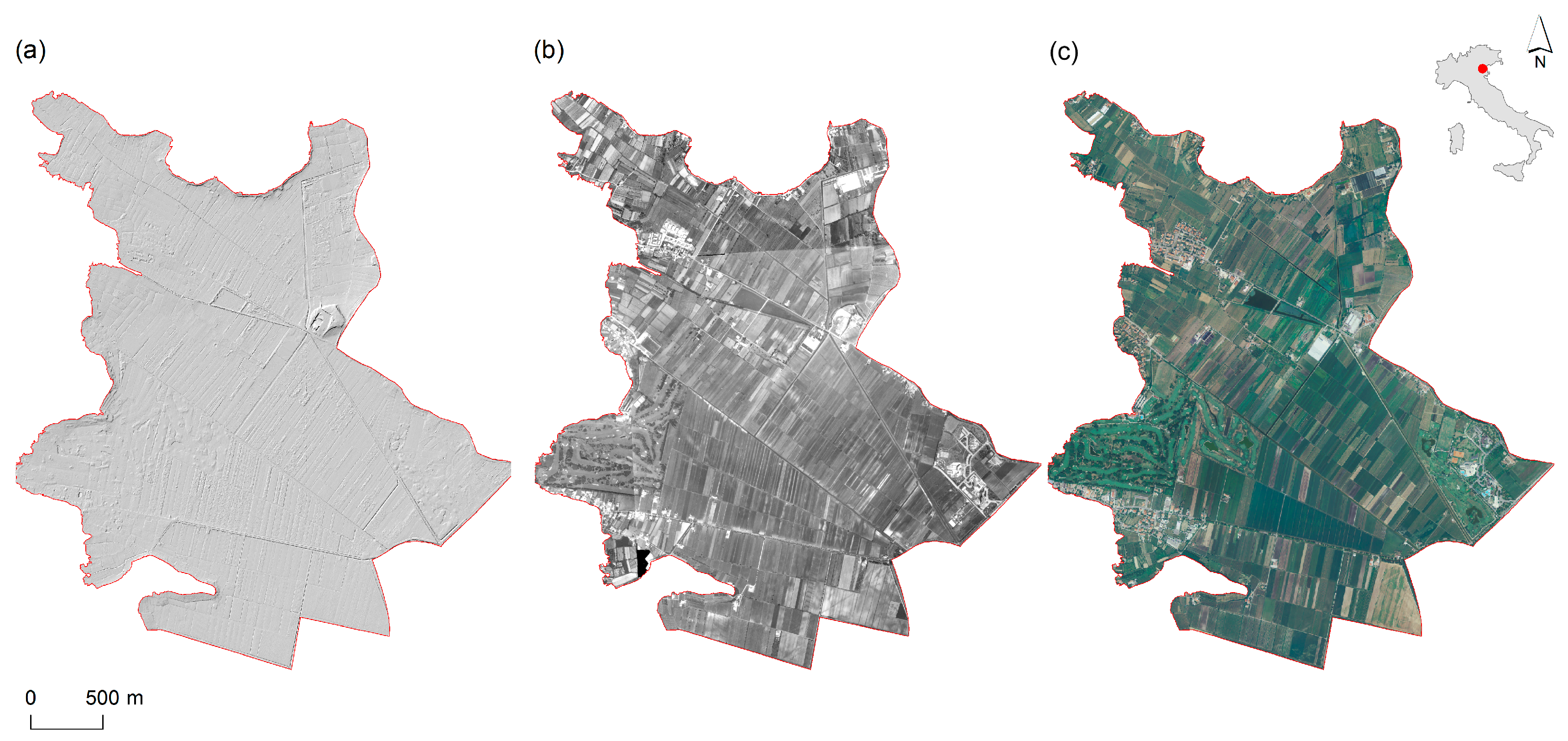
Figure 2.
Hyetographs simulated for the calculation of the updated Network Saturation Index (uNSI). Hyetographs include: a dimensionless rainfall (Sym01) [47], hyetographs for rainfalls of 1, 2, 4, 8, 24, 48, 72, 168, 240 h (Sym02 to Sym09 respectively) [48], the SCS/NRCS hydrographs (type I (for a design storm of 24 and 48 h), type Ia (for 24 h), type II (for a design storm of 24 and 48 h) and type III (for 24 h)) (Sym10 to Sym15 respectively) [49], and two more hyetographs proposed for a rainfall of 72 and 96 h (Sym16 and Sym17) [50].

Figure 3.
Simulated hyetograph for Sym01 for an event having a return period of 2 years, duration of ~1 h and cumulative rainfall of ~32.5 mm; the effective rainfall producing runoff for different antecedent moisture conditions is shown in red.
Figure 3.
Simulated hyetograph for Sym01 for an event having a return period of 2 years, duration of ~1 h and cumulative rainfall of ~32.5 mm; the effective rainfall producing runoff for different antecedent moisture conditions is shown in red.

Figure 4.
Drainage density (Drainden) and Storage Capacity (Storcap) in 1983 and 2010, and relative differences.
Figure 4.
Drainage density (Drainden) and Storage Capacity (Storcap) in 1983 and 2010, and relative differences.

Figure 5.
(a–f) Drainage density (Drainden) (left panel) and Storage Capacity (Storcap) (middle panel) in 1983 and 2010, and overview of the landscape (right panel) for the same years. The figure exemplifies changes in the sizes of the plot, and changes in the network system, and the resulting characteristics of the network.
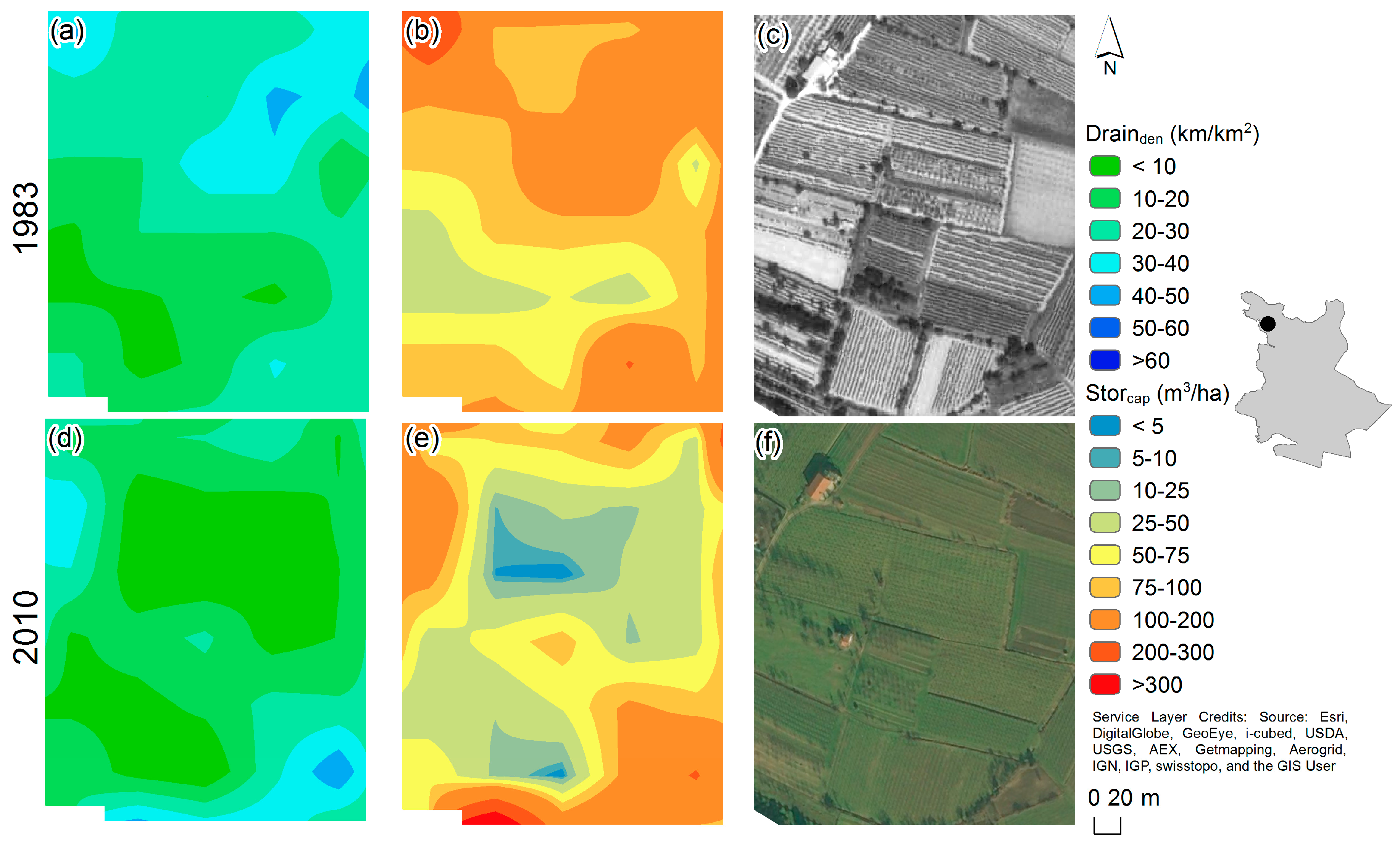
Figure 6.
Average ponding time for the considered soil. Ponding time (evaluated considering all hyetograph types) as a function of the Return Period (a) averaged for each of the considered antecedent soil moisture condition (0 to 100% saturation), and (b) averaged considering all saturation conditions. (c) average ponding time considering all hyetograph types and return periods as a function of the antecedent soil moisture condition (saturation). In (b) and (c) different prediction bounds for Equation (4) are shown: BoundOB describes yn+1(x), for all x, while BoundF shows the fitted equation for all x. Note that the intervals associated with a new observation (OB) are wider than the fitted function (F) intervals because of the additional uncertainty in predicting a new response value (the curve plus random errors). Note that in (a), 0% and 1% saturation overlap, presenting minimal differences.

Figure 7.
Average difference in uNSI between 2010 and 1982. A negative sign indicates a faster response of the network in 2010. Differences in uNSI (evaluated considering all hyetograph types) as a function of the Return period (a) averaged for each of the considered antecedent soil moisture condition (0 to 100% saturation), and (b) averaged considering all saturation conditions. (c) Average difference between uNSI considering all hyetograph types and return periods as a function of the antecedent soil moisture condition (saturation). In (b) and (c) different prediction bounds are shown: BoundOB describes yn+1(x), for all x, while BoundF shows the fitted equation for all x. Note that the intervals associated with a new observation (OB) are wider than the fitted function (F) intervals because of the additional uncertainty in predicting a new response value (the curve plus random errors).

Figure 8.
Estimated effects on the response (ponding time (a) and ΔuNSI (b)) from changing each predictor value (percentage of the total storm period that has occurred at the start of the heaviest burst—BrLoc%, number of bursts—Brn, hyetograph triangularity—TRN, asymmetry of the storm—asym), averaging out the effects of the other predictors. Values of the predictors are chosen automatically to produce a relatively large effect on the response.
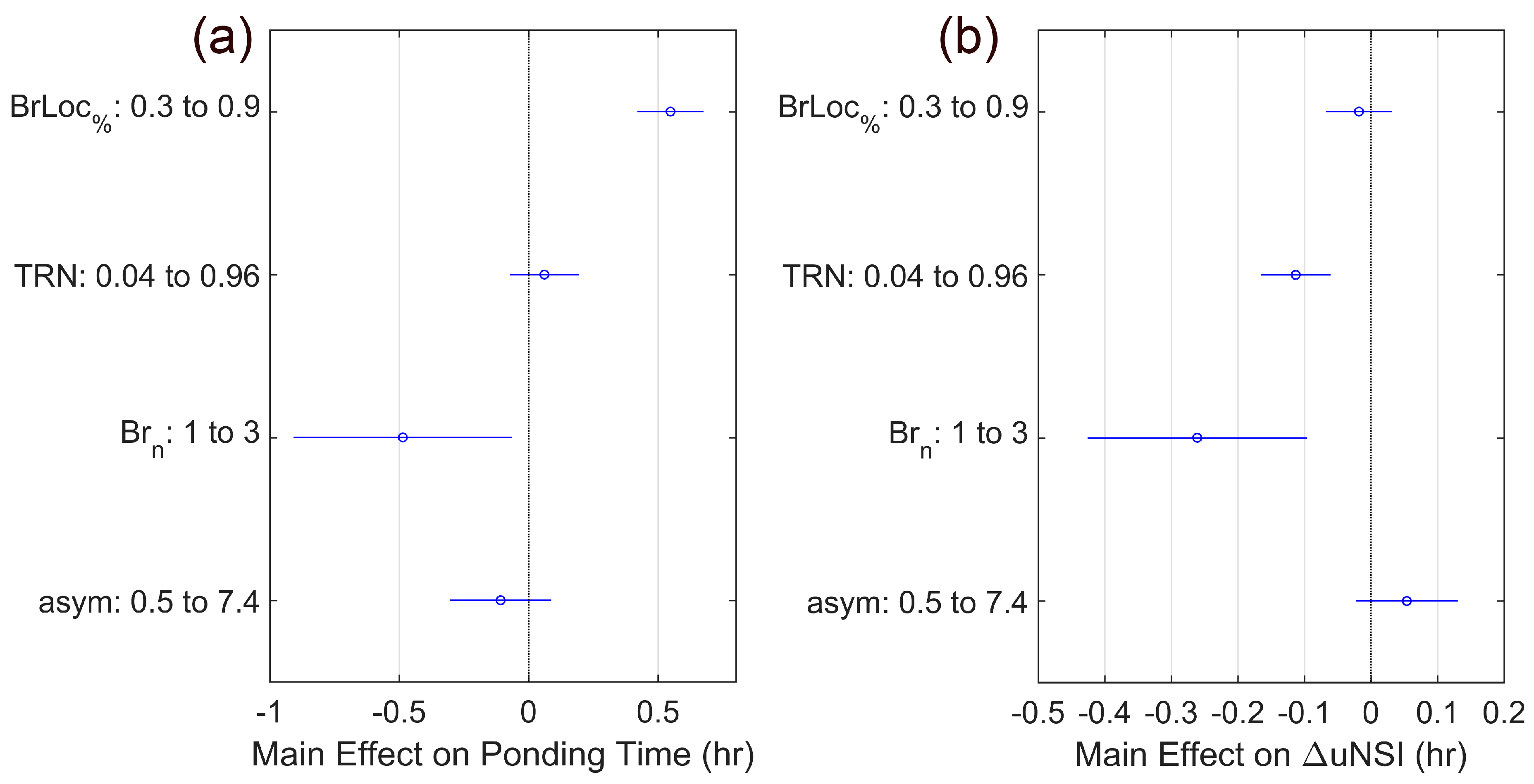
Figure 9.
Estimated effects on ponding time of keeping one predictor fixed (percentage of the total storm period that has occurred at the start of the heaviest burst—BrLoc%, number of bursts—Brn, hyetograph triangularity—TRN, asymmetry of the storm—asym) while varying the other. The average effect is shown as a circle, while the horizontal bars are showing the confidence interval for the estimated effect. The blue symbols represent the overall average effect obtained by changing one predictor independently from the other, while the red ones represent the average effect achieved by changing one predictor over different values of the other one.
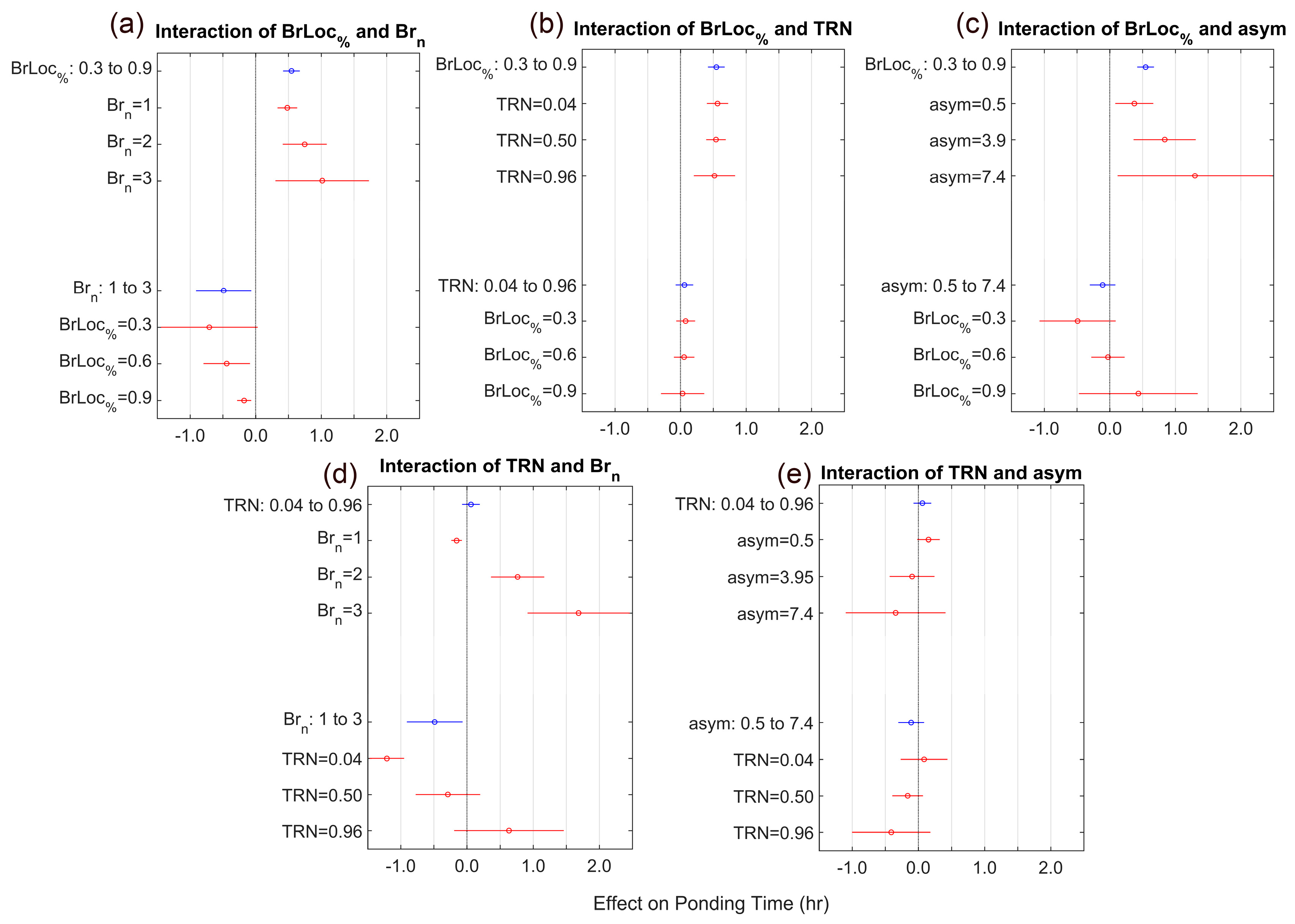
Figure 10.
Estimated effects on ΔuNSI of keeping one predictor fixed (percentage of the total storm period that has occurred at the start of the heaviest burst—BrLoc%, number of bursts—Brn, hyetograph triangularity—TRN, asymmetry of the storm—asym) while varying the other. The average effect is shown as a circle, while the horizontal bars are showing the confidence interval for the estimated effect. The blue symbols represent the overall average effect obtained by changing one predictor independently from the other, while the red ones represent the average effect achieved by changing one predictor over different values of the other one.

Figure 11.
Local difference in uNSI between 2010 and 1982. A negative sign indicates a faster response of the network in 2010. Differences are evaluated considering all hyetographs and (a–c) all return periods averaged for each specified antecedent soil moisture condition (Sat); (d–f) all saturation conditions averaged for the specified return period (Rp); and (g) displays some characteristics of the urbanisation settings and regulations for the area [27].
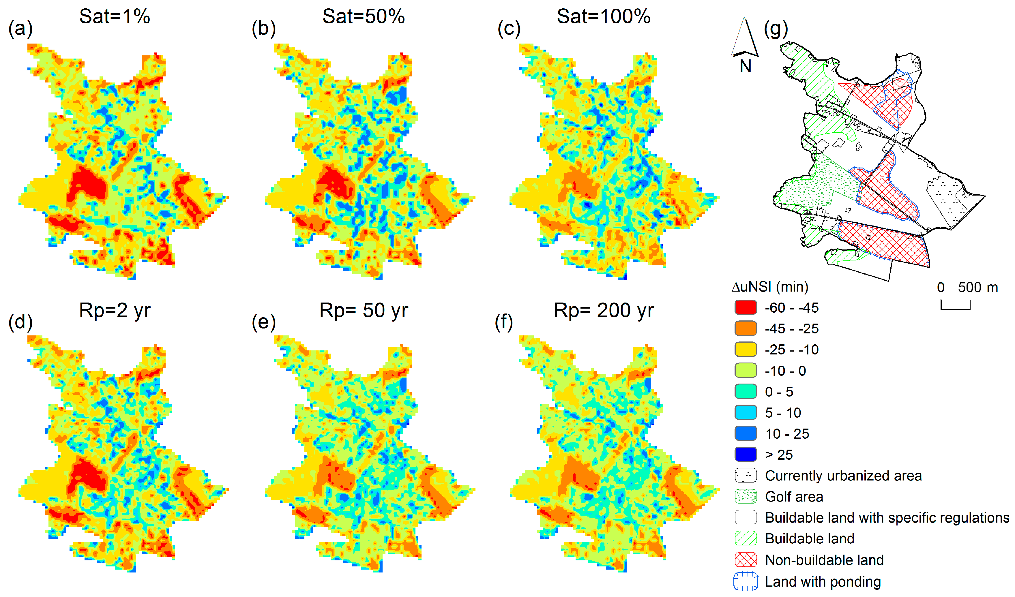

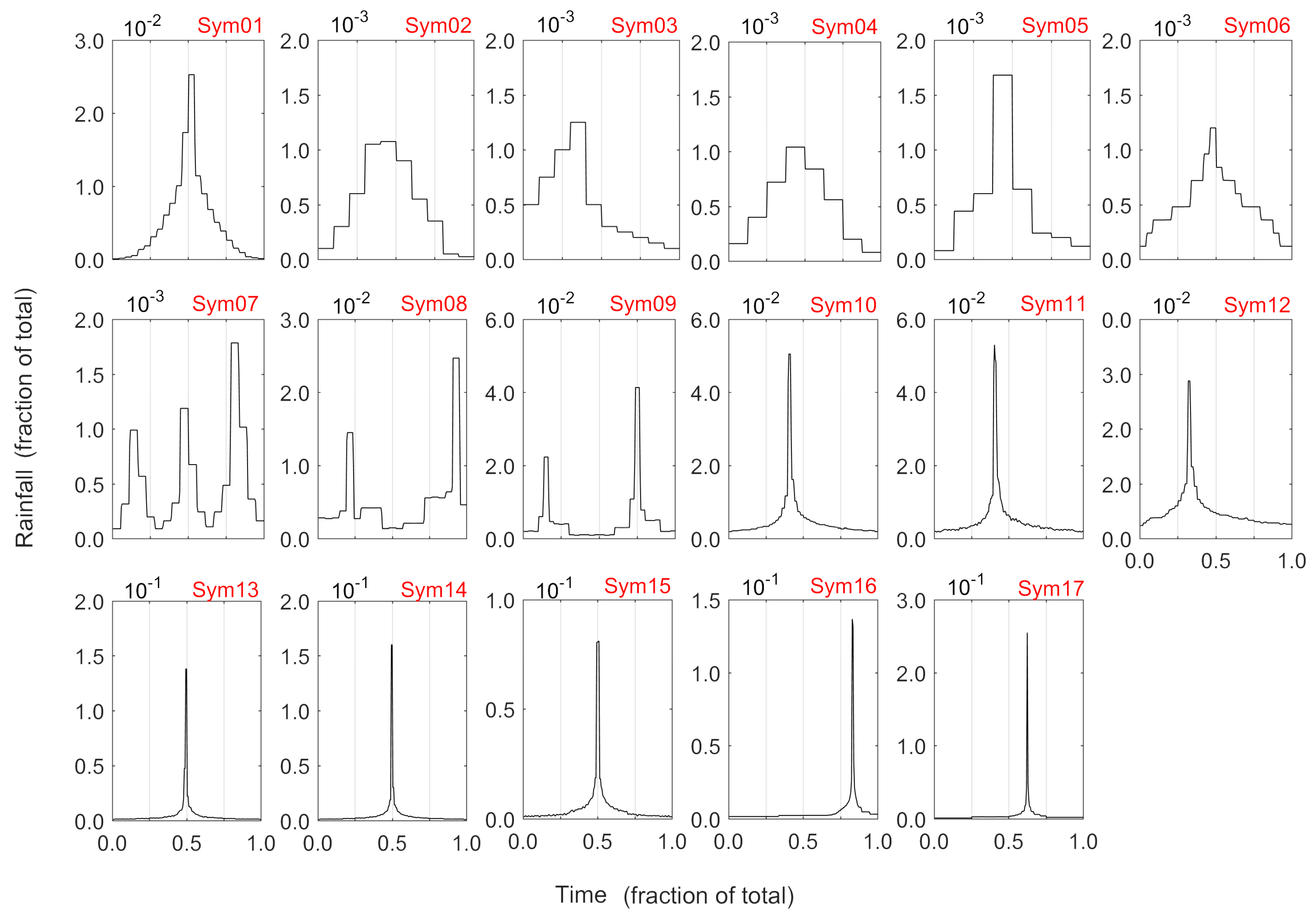
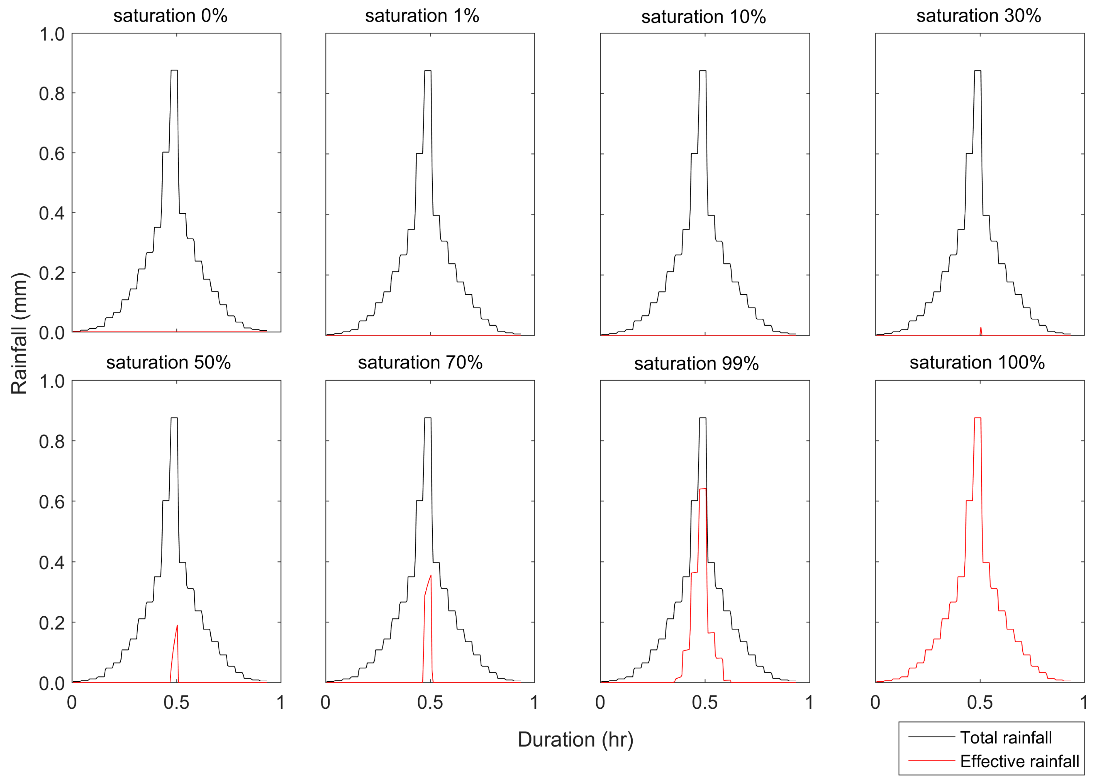
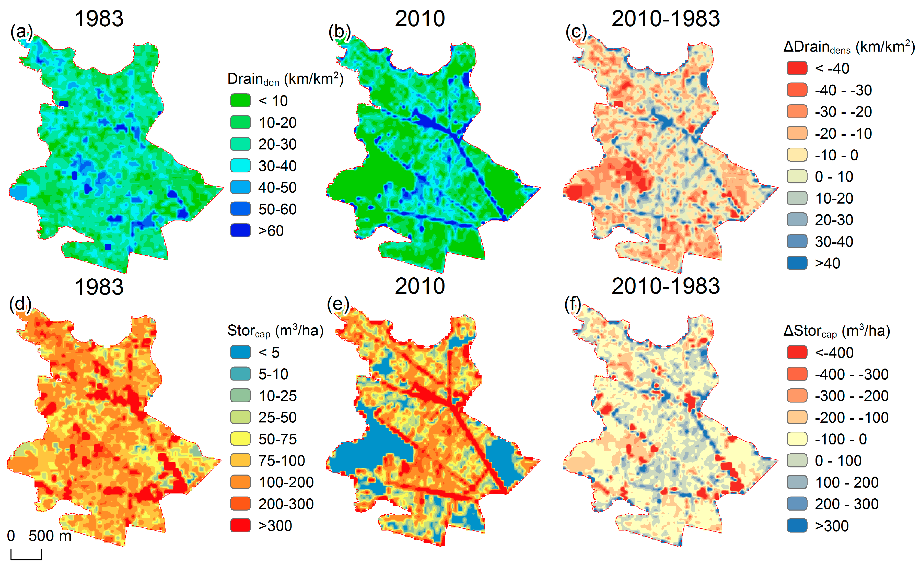
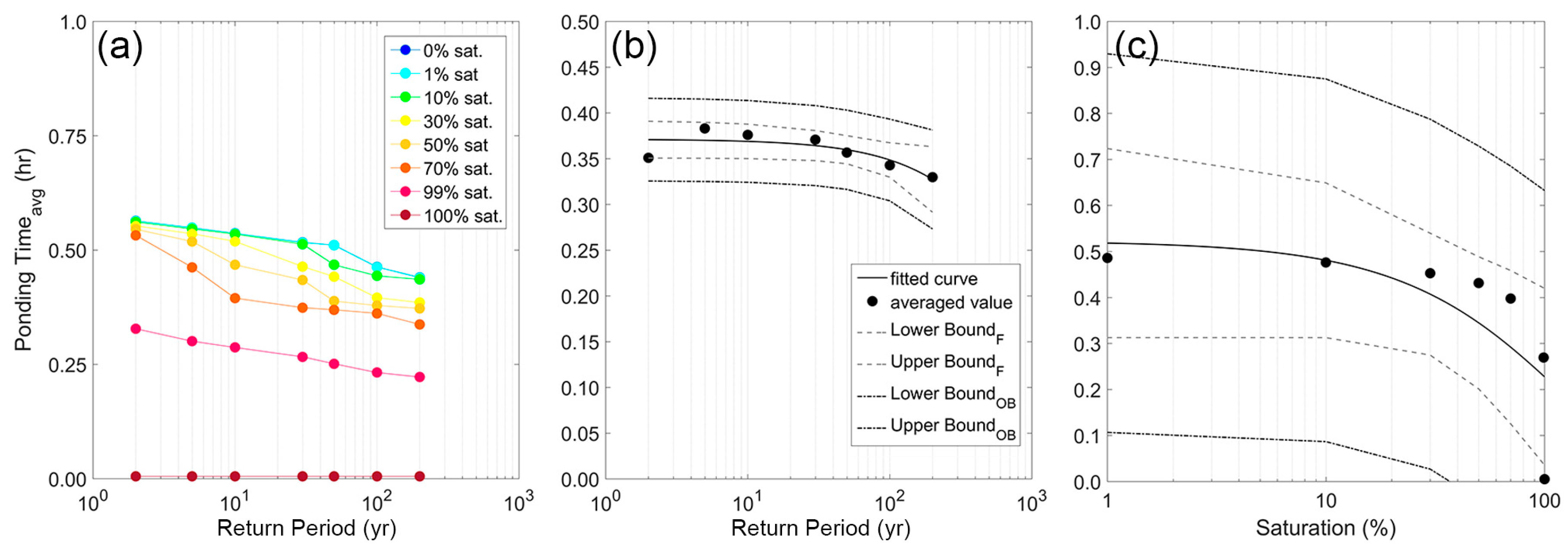
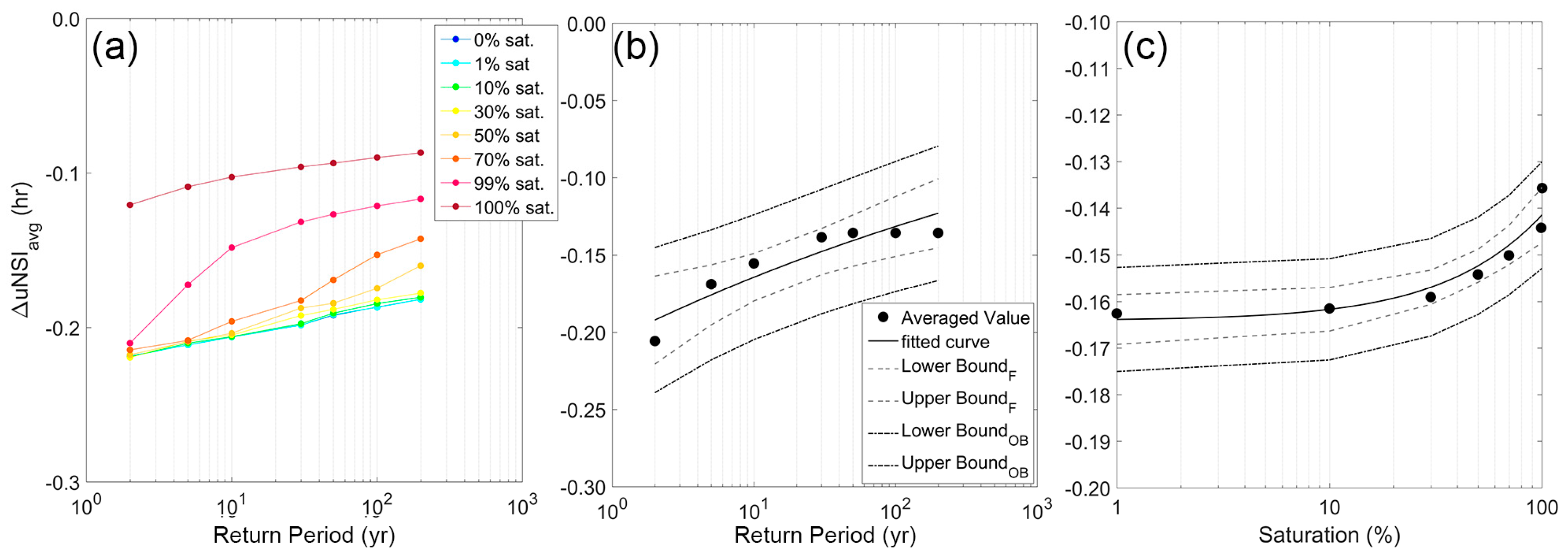
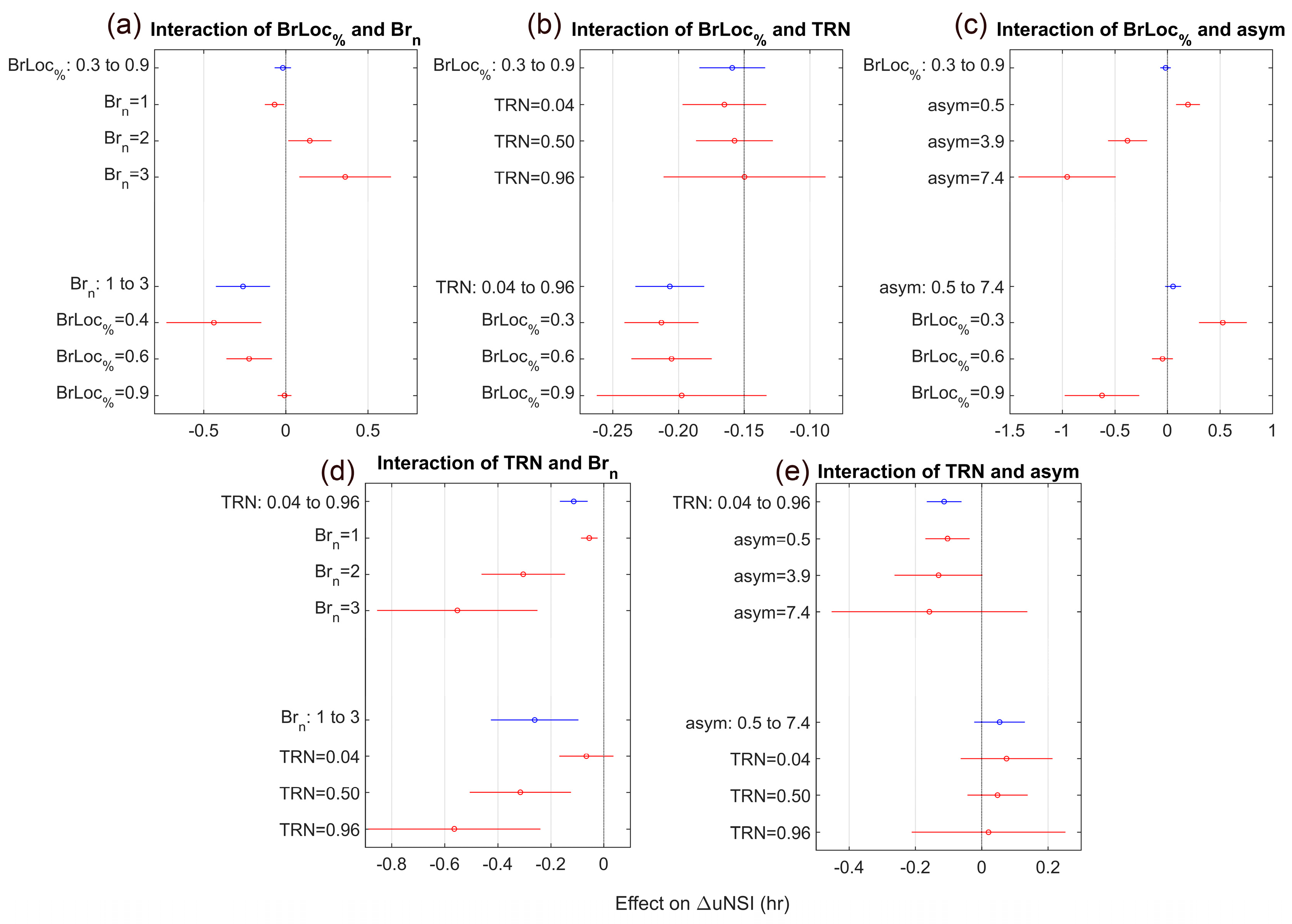
Table 1.
Main soil characteristics that are available for the study area [28].
| Parameter | Value | |
|---|---|---|
| Effective hydraulic conductivity | Ks | 43.79 mm·h−1 |
| Matric pressure at the wetting front | Ψf | 130 mm |
| Saturated moisture content | θs | 0.63 |
Table 2.
Classification of the hyetographs according to the four defined criteria: location of the heaviest burst within the storm period (BrLocqtl), percentage of the total storm period that has occurred at the start of the heaviest burst (BrLoc%), number of bursts (Brn), hyetograph triangularity (TRN), asymmetry of the storm (asym).
| BrLoc% | Brn | TRN | Asym | |
|---|---|---|---|---|
| Sym01 | 0.5 | 1 | 0.4 | 1.8 |
| Sym02 | 0.5 | 1 | 0.9 | 1.5 |
| Sym03 | 0.4 | 1 | 0.8 | 1.5 |
| Sym04 | 0.5 | 1 | 1.0 | 1.3 |
| Sym05 | 0.4 | 1 | 0.6 | 1.0 |
| Sym06 | 0.5 | 1 | 0.8 | 0.9 |
| Sym07 | 0.8 | 3 | 0.6 | 3.0 |
| Sym08 | 0.9 | 2 | 0.4 | 7.4 |
| Sym09 | 0.8 | 2 | 0.2 | 2.1 |
| Sym10 | 0.4 | 1 | 0.2 | 0.6 |
| Sym11 | 0.4 | 1 | 0.2 | 0.6 |
| Sym12 | 0.3 | 1 | 0.3 | 0.5 |
| Sym13 | 0.5 | 1 | 0.1 | 1.1 |
| Sym14 | 0.5 | 1 | 0.1 | 1.6 |
| Sym15 | 0.5 | 1 | 0.1 | 1.9 |
| Sym16 | 0.8 | 1 | 0.1 | 1.8 |
| Sym17 | 0.6 | 1 | 0.0 | 1.7 |
Table 3.
Fitted coefficients, 95% confidence intervals (CI95) and goodness of fit (R2 and Root Mean Square Error—RMSE) for Equation (4) when considering the ponding time (PT) as a function of the return period or the saturation condition.
| PT = f (Return Period) | PT = f (Saturation Condition) | |
|---|---|---|
| a | 0.37 (CI95 = 0.36, 0.39) | 0.52 (CI95 = 0.36, 0.68) |
| b | −6.29 × 10⁻⁴ (CI95 = −1.14 × 10⁻³, 1.18 × 10⁻⁴) | −0.83 (CI95 = −1.61, −0.04) |
| RMSE | 0.01 h | 0.1 h |
| R2 | 0.68 | 0.62 |
Table 4.
Fitted coefficients, 95% confidence intervals (CI95) and goodness of fit (R2 and Root Mean Square Error—RMSE) for Equation (4) when considering the ΔuNSI (difference between the network response in 2010 vs. 1983) as a function of the return period or as a function of the saturation condition.
| ΔuNSI = f (Return period) | ΔuNSI = f (Saturation condition) | |
|---|---|---|
| a | −0.19 (CI95 = −0.21, −0.18) | −0.17 (CI95 = −0.18, −0.16) |
| b | −1.33 × 10⁻³ (CI95 = −1.23 × 10⁻³, 3.37 × 10⁻⁴) | −0.15 (CI95 = −0.19, −0.11) |
| RMSE | 0.01 h | 0.003 h |
| R2 | 0.72 | 0.92 |
© 2017 by the authors. Licensee MDPI, Basel, Switzerland. This article is an open access article distributed under the terms and conditions of the Creative Commons Attribution (CC BY) license ( http://creativecommons.org/licenses/by/4.0/).
Share and Cite
MDPI and ACS Style
Sofia, G.; Tarolli, P. Hydrological Response to ~30 years of Agricultural Surface Water Management. Land 2017, 6, 3. https://doi.org/10.3390/land6010003
AMA Style
Sofia G, Tarolli P. Hydrological Response to ~30 years of Agricultural Surface Water Management. Land. 2017; 6(1):3. https://doi.org/10.3390/land6010003
Chicago/Turabian StyleSofia, Giulia, and Paolo Tarolli. 2017. "Hydrological Response to ~30 years of Agricultural Surface Water Management" Land 6, no. 1: 3. https://doi.org/10.3390/land6010003
Note that from the first issue of 2016, this journal uses article numbers instead of page numbers. See further details here.