
Modeling Future Urban Sprawl and Landscape Change in the Laguna de Bay Area, Philippines
by
 ,
,
Kotaro Iizuka
1,*, 
Brian A. Johnson
2 ,
,
Akio Onishi
3,
Damasa B. Magcale-Macandog
4,
Isao Endo
2 and
Milben Bragais
4 1
Center for Southeast Asian Studies (CSEAS), Kyoto University, 46, Yoshida Shimoadachicho, Sakyo-ku Kyoto-shi, Kyoto 606-8501, Japan
2
Institute for Global Environmental Strategies (IGES), 2108-11 Kamiyamaguchi, Hayama, Kanagawa 240-0115, Japan
3
Faculty of Environmental Studies, Tokyo City University, 3-3-1 Ushikubo-nishi, Tsuzuki-ku, Yokohama, Kanagawa 224-8551, Japan
4
Institute of Biological Sciences, University of the Philippines Los Baños, College, Laguna 4031, Philippines
*
Author to whom correspondence should be addressed.
Land 2017, 6(2), 26; https://doi.org/10.3390/land6020026
Submission received: 6 March 2017
/
Revised: 10 April 2017
/
Accepted: 11 April 2017
/
Published: 14 April 2017
(This article belongs to the Special Issue Urban Land Systems: An Ecosystems Perspective)
Abstract
:This study uses a spatially-explicit land-use/land-cover (LULC) modeling approach to model and map the future (2016–2030) LULC of the area surrounding the Laguna de Bay of Philippines under three different scenarios: ‘business-as-usual’, ‘compact development’, and ‘high sprawl’ scenarios. The Laguna de Bay is the largest lake in the Philippines and an important natural resource for the population in/around Metro Manila. The LULC around the lake is rapidly changing due to urban sprawl, so local and national government agencies situated in the area need an understanding of the future (likely) LULC changes and their associated hydrological impacts. The spatial modeling approach involved three main steps: (1) mapping the locations of past LULC changes; (2) identifying the drivers of these past changes; and (3) identifying where and when future LULC changes are likely to occur. Utilizing various publically-available spatial datasets representing potential drivers of LULC changes, a LULC change model was calibrated using the Multilayer Perceptron (MLP) neural network algorithm. After calibrating the model, future LULC changes were modeled and mapped up to the year 2030. Our modeling results showed that the ‘built-up’ LULC class is likely to experience the greatest increase in land area due to losses in ‘crop/grass’ (and to a lesser degree ‘tree’) LULC, and this is attributed to continued urban sprawl.
1. Introduction
Urban sprawl is occurring at an accelerated pace in many developing countries worldwide due to rapid global economic and population growth coupled with globalization. Currently, 54% of the world’s population lives in urban areas, and the United Nations has predicted that by 2050, 66% of the world’s population will live in urban areas [1]. This rapid increase in urban population has forced nations to meet the changing demands for necessities such as food, energy, land, and water. A major concern related to this urban sprawl is land-use (LU)/land-cover (LC) change, which can dramatically alter the landscape in areas with high rates of urban expansion [2]. These LULC changes are often based on the plans of local governments to increase economic development and to support their growing populations. However, such plans may fail to consider other factors, including climate conditions, water resources, and food security [3,4]. Since population increases are expected to continue in many developing countries, governments need to take appropriate action to ensure that urbanization measures consider these factors. Thus, policymakers need to understand the historical trends in LULC change and must visualize future LULC scenarios to ensure the safety and standard of living of the residents [4]. LULC changes and related problems will likely continue to be major issues in the future [5,6], and, for governments to strategically plan future LULC development, they need to estimate the locations of LULC changes, the time scale of occurrence, and the factors driving these changes [7,8,9]. It is difficult to monitor LULC changes over large areas using field surveys or other ground-level data collection approaches, so many studies have instead detected and mapped LULC changes from above using satellite or aerial remote sensing data [2,10,11].
Nowadays, a great deal of attention is being paid in particular to rapidly growing cities in southeast Asia (and other regions), with the goal of understanding relationships between LULC changes and other factors such as climate change [12] and forestry [13]. The Metro Manila area of the Philippines is one of the most rapidly growing mega cities in the world [2], and, among other things, Manila’s urban sprawl has threatened the ecology of the agricultural lands located along the urban fringe [14] and increased flood vulnerability in the area [15]. Other impacts related to food security are also likely to emerge in this area if agricultural lands keeps decreasing and the population keeps increasing [16]. Additionally, if Manila’s urban sprawl continues into the remaining forest/agro-forest areas surrounding the city, various ecosystem services provided by these forest systems [17] will cease or decline, while, if the forested areas are instead converted to agricultural lands, it may lead to land degradations that also significantly impact the environment (e.g., increased erosion) [18,19]. Urbanization-related issues have large impacts on both human and environmental well-being, and it is clear that development in the region is causing various problems for both people and the environment. Thus, the LULC change trends in such a rapidly developing region should be monitored, and future LULC changes should be estimated to assess the impacts of future LULC changes.
The Laguna de Bay, located to the southeast of Metro Manila, is the largest lake in the Philippines and an important source of water for the population of Metro Manila and the surrounding cities and towns. Several river basins drain into this lake, and the LULC conditions of these drainage basins can have a significant effect on the lake water quality and quantity owing to different rainfall-runoff rates and pollutant loads of different LULC types [20]. Previous LULC change modeling studies in this region have focused mostly on the Metro Manila area [14,15,21,22], which does not give the full picture of the changes affecting the lake. Some past studies have also focused on specific drainage basins of the lake [19,23], but few works have studied the LULC changes of the entire surrounding landscape of the Laguna de Bay. According to the Global Footprint Network [24] Ecological Footprint Report, the Laguna lake watershed has undergone LULC changes during the last 30 years, wherein large rural areas have been converted into commercial, residential, and industrial areas. It was noted that the major LULC change occurred between 2003 and 2010, when the built up areas increased by 116%. During this period, the closed forests, observed mostly in the west, northwest, and southern parts of the lake, were reduced by 35% [25]. The lake has been the catch basin of much of the runoff from Metro Manila, so it has been heavily impacted by Metro Manila’s urbanization and population increase. As Metro Manila has developed, the lake’s water quality has deteriorated owing to increases in agricultural, industrial, and domestic pollution. Moreover, previous studies have reported that 66% of the lake watershed is vulnerable to erosion caused by urban growth, deforestation, and mining activities. Further, about four million tons of suspended solids flow into the lake annually [26]. From such perspectives, several local governments based along the lake as well as the national Laguna Lake Development Authority (a national government agency) have expressed interest in future LULC predictions and maps.
Using historical data, we can obtain information on past LULC changes that can be used to help model future LULC changes [11,27,28,29]. LULC change modeling for territorial planning has a long history, and a variety of modeling methods have been assessed at various locations, time periods, and spatial scales/spatial resolutions [30]. In the general sense, land change approaches can be roughly categorized into six types of approaches [31]; machine learning and statistical, cellular automata, sector-based economic, spatially disaggregated economic, agent-based, and hybrid approaches. In this work, we focused on the machine learning category, namely the Multilayer-Perceptron (MLP) Artificial Neural Network (ANN) approach, which is gaining attention for modeling LULC changes. ANN are powerful tools for modeling complex behaviors [32] (e.g, relationships between land transitions and their driving forces), and the usage of ANN for LULC change modeling has increased in recent years. As one example, Grekousis et al. [33] demonstrated the use of ANN to model future urban growth based on demographic time-series data. Triantakonstantis and Stathakis [32] used MLP for modeling future LULC transition probabilities based on information on past LULC changes and geomorphic drivers such as elevation, slope, and distance variables from specific land features, etc. Similar methods can be seen in a number of studies, although the number and types of driver variables utilized vary [27,34,35,36,37,38].
Past studies have been conducted at various geographical locations and spatial extents, e.g., the city level or provincial level. However, not many works have used the MLP method for modeling complex larger regions. In our case, we have focused on a larger ecological scale that encompasses multiple municipalities and provinces, each of which have different development policies, infrastructure, topography, climatic conditions, etc. Therefore, the MLP method for modeling the LULC transitions throughout the region becomes a strong decision tool, even when prior knowledge is lacking [31,37], and this is one of its advantages compared to other methods like SLEUTH (Slope, Land use map, Excluded area, Urban area, Transportation map, Hillside area), which require coefficient values to be set [39], and other cellular automata methods that require a suitability map [40] based on prior knowledge of change behavior. MLP can also handle a large number of data sets, so it could be a good predictor for recognizing the patterns of the changes in the area.
Our main objective in this study is to model the future LULC changes in the river basins that drain into the Laguna de Bay up to year 2030. This work implements the MLP with the Markov Chain method embedded in the Land Change Modeler (LCM) of the TerrSet software package [41]. This model is based on transition probabilities calculated using historical LULC change data and other freely/openly available geospatial datasets.
2. Study Area
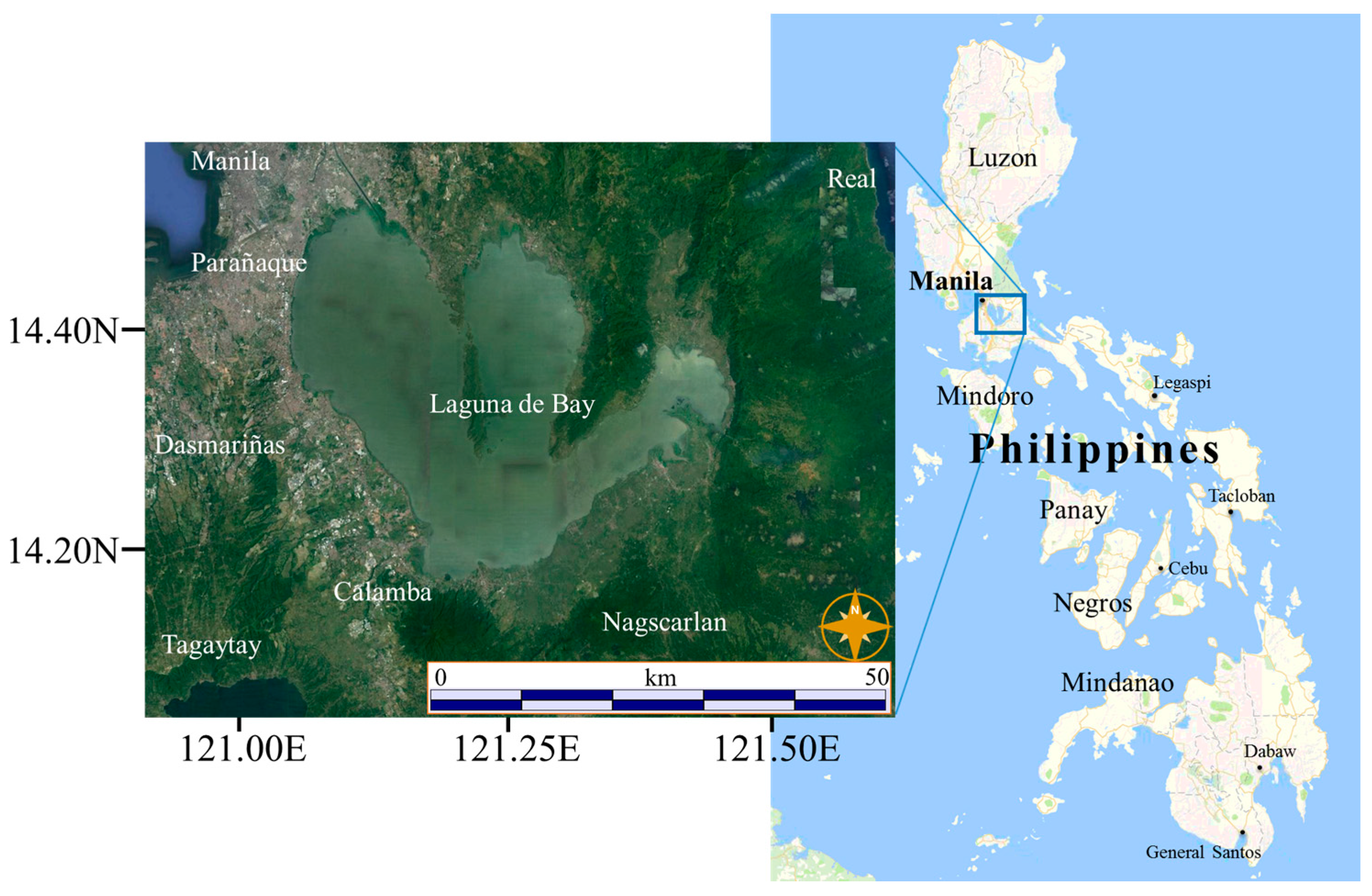
The Philippines is one of the most rapidly developing countries in Asia. In particular, the Metropolitan Manila area has experienced large and rapid LULC changes owing to urban area expansion [2,6]. The Laguna de Bay, located just southeast of Manila, is the largest and most important and dynamic lake in the Philippines owing to its vital economic, political, and socio-cultural significance. With a surface area of 900 km2, this lake is also one of the largest in Southeast Asia. From the 21 major river systems, more than 100 rivers that traverse the 292,000 ha watershed flow into the lake. The study area includes the municipalities surrounding the Laguna de Bay, located southeast of Metro Manila. Figure 1 shows that Metro Manila, situated to the northwest, has a denser urban concentration; while smaller, less densely populated cities and municipalities can be seen in the west and southwest areas surrounding the Laguna de Bay. The population of this area was estimated to be about 15 million in 2010 [42]. Agricultural lands are distributed mainly along the southwestern, southeastern, and northeastern shores of the lake. Large forest areas are located on the east side of the lake with mountain ranges (300–600 m), the highest peak of which, Mt. Banahao (2170 m), is located southeast of the lake. Just south of Laguna de Bay, Mt. Makilling (1090 m) is seen. The area is broad and the climate varies along different provinces of the area. Average annual temperatures are cooler in the mountainous areas (23 °C) than in the lower altitude plains and cities (25 °C and 27 °C respectively). Annual precipitation ranges from over 3000 mm in the east mountainous areas to 1900 mm in the western area around Manila bay. The area in focus is approximately 60 km × 80 km in the north-south and east-west directions, respectively, and it was chosen to visualize how urban sprawl will affect the LULC in the areas surrounding the Laguna de Bay. Therefore, we have ignored the center and northern areas of Metro Manila, even though it also experienced urban sprawl.
3. Materials and Methods
3.1. Overview
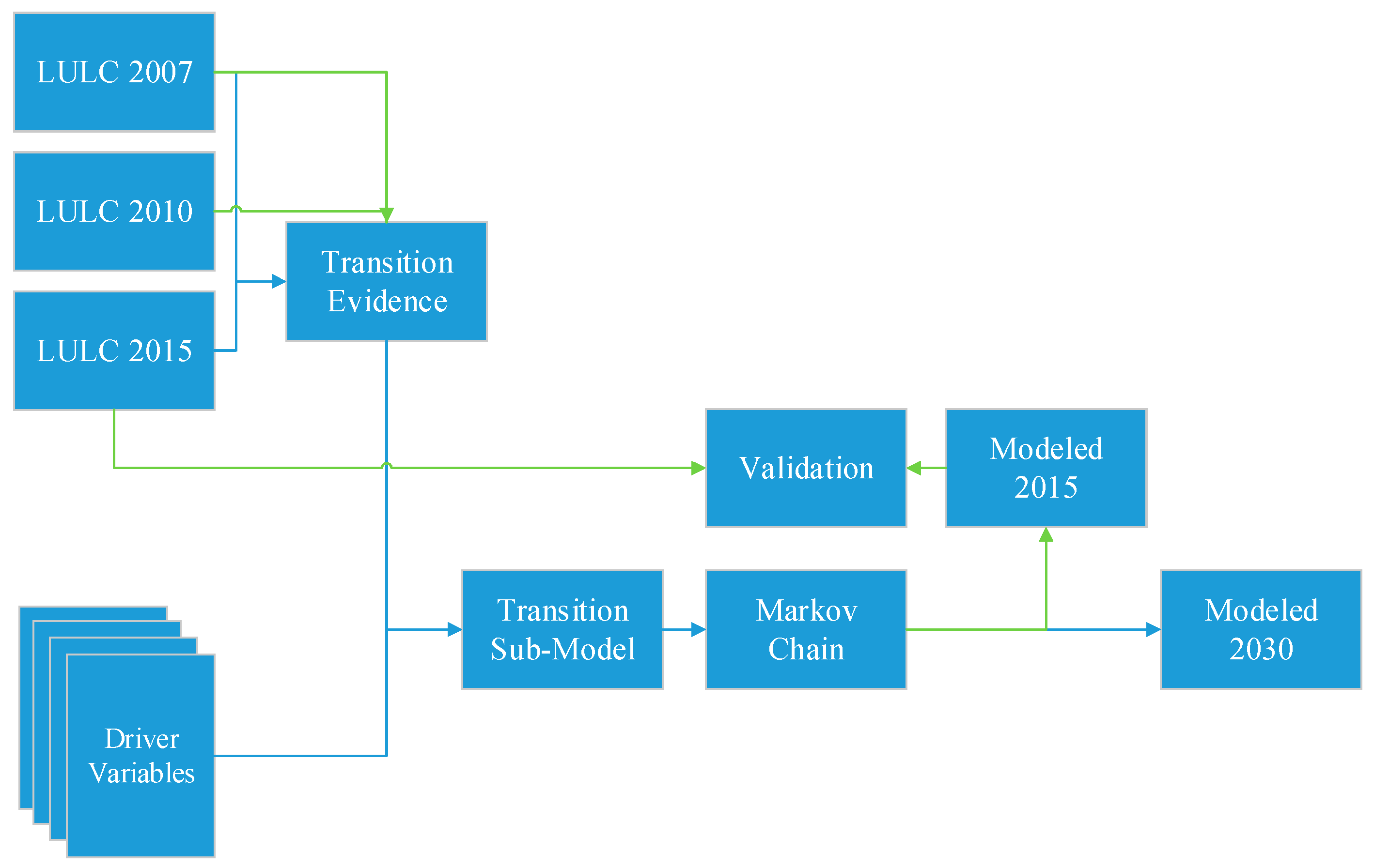
As shown in Figure 2, the overall flowchart of the study details three main steps in generating maps of future LULC. The first step is to gather evidence of past LULC transitions by identifying the historical LULC changes in the area. For this, a map of recent LULC change from 2007 to 2015 was generated by using optical and synthetic aperture radar (SAR) satellite images from 2007 and 2015 and automated image classification techniques. Four LULC classes, including Built-up, Forests, Crop-Grass, and Water Bodies, were mapped for each year, and the LULC changes between 2007 and 2015 were identified by overlaying the two maps. The full details of the LULC change mapping methodology employed in this study are given in Johnson et al. [44], although brief information will be stated about the methods and the result of the developed LULC change map. In the second step, drivers of these historical LULC changes were identified by using various ancillary spatial datasets containing demographic, topographic, and climate information. In the third and final step, the future LULC of the area (2030) was modeled and mapped by using Markov Chain analysis.
In addition to the main procedure, the validity of the LULC change model was examined by comparing a ‘simulated 2015 LULC map’ with a ‘reference 2015 LULC map’. The ‘simulated 2015 LULC map’ was generated using similar methods to those mentioned above. First, LULC maps from the years 2007 and 2010 were utilized along with the ancillary spatial datasets to model the LULC conditions in the year 2015 LULC (i.e., simulated 2015 LULC map). This map was then compared with the actual (i.e., reference) 2015 LULC map.
3.2. LULC Maps of 2007, 2010 and 2015
To develop a categorical LULC change map of the study area, we utilized optical (Landsat 5 and Landsat 8) and synthetic aperture radar (ALOS PALSAR-1 and PALSAR-2) satellite images from the years 2007, 2010, and 2015 and classified the pixels in the images from each year into one of four LULC classes (Built-up, Crop-Grass, Trees, and Water) using a semi-unsupervised classification approach [44]. Crop-Grass includes cropland, paddy fields, grassland, and pasture (however the majority lies within paddy and other agriculture). Trees includes forest and agroforestry plantations (e.g., coconut, banana, etc.). This four class LULC classification system, although relatively simple, was chosen because it was representative of the area and allowed us to maintain a relatively high LULC change mapping accuracy (adding more specific LULC classes usually decreases LULC mapping accuracy, and LULC change mapping accuracy even more so due to error propagation). The overall accuracy of the 2007–2015 LULC change map was estimated as 90.2%.
3.3. Evidence of LULC Change Transition
By using the two different periods of the LULC change maps, the net change in area of each LULC class was calculated, and the spatial distributions of all of the LULC changes were analyzed. The areas of transition and persistence of each LULC type within the 2007–2015 analysis was for both training and validation data with all of the driver variables when performing transition sub-modeling.
3.4. Collection and Processing of Data on Potential Driver Variables
Spatial data related to various potential drivers of LULC change were collected via the Internet. Only datasets which were openly available online were used, so our modeling approach can easily be replicated by other researchers. The drivers influencing LULC change processes are extremely diverse as well as highly variable from one location to another [45,46]. What is known is that the changes are typically the results of the local population’s responses to economic opportunities [45], which gives relevance to various contextual features such as the distance from a location to nearby infrastructural features like major roads, town centers, and so forth, and many works show these kind of factors to be used as potential drivers for calibrating the change probability. These context features are also considered in this work for the model calibration. However, as mentioned before, we are not so aware of all the LULC change drivers in the area, so we want to shed some light on the question of ‘What factors influence the LULC transitions?’ Thus, data for a large number of possible drivers was collected to test which variables had the greatest levels of influence on LULC changes (a brief explanation is made later for why each variable was considered as potentially relevant). Table 1 shows the complete list of collected data related to these drivers; not all of these datasets were selected for the final LULC modeling.
Gridded climate data with a 1 km resolution was obtained from the Philippine GIS Data Clearinghouse (PhilGIS) [47] (the original global dataset is distributed at WorldClim [52]). We included all of the climate data that was processed in the form of bioclimatic variables [53,54]. These climate variables can be considered drivers of LULC change because the agro-climatic zones with different climatic conditions can affect the suitability of agricultural lands for its productivity [55]; thus, no patterns of change in the preferred area might be identified relative to this factor. This is one challenge in our work since not many related studies implement climatic information in their calibration. The reason can be considered that, depending on the scale of the study area, the spatial variation of climatic factors might be too small to have any influence on LULC changes. However, our study area encompasses areas with different climatic conditions, which may allow us to identify if climate is affecting LULC change. Topographic data including elevation, slope, and aspect were obtained from the Shuttle Radar Topography Mission (SRTM) 1 s (30 m) digital elevation model (DEM) [48]. Topography is often a significant driver of LULC change [56] because areas with steep slopes are typically more difficult and thus less likely than flatter areas to be converted to built-up land or cropland. The SRTM DEM contains only elevation information; therefore, gridded slope and aspect data were generated by using the TerrSet software package [41]. Road and waterway data through March 03, 2016, were collected from OpenStreetMap (OSM) [49], and a 25 m grid map containing the Euclidean distance of each pixel to the nearest road/waterway was calculated by using TerrSet software [41]. The distance from roads in addition to other various LULC context features are often drivers of LULC change because more developed road networks are found with a greater rate of conversion [57]. This study focuses not only on the roads in general but also on different types/functions of roads by separating roads into detailed classes. It is expected that the importance of different road types could further distinguish the patterns of transitions throughout the study region. The case is similar for the waterways. Nightlight intensity information in the form of monthly average radiance composite images was obtained from the Visible Infrared Imaging Radiometer Suite (VIIRS) and Global Defense Meteorological Satellite Program-Operational Linescan System (DMSP-OLS) nighttime lights time series dataset [50]. The nightlight changes from 2007 to 2015 were computed by performing radiometric normalization of the images to ensure that the 2007 data had a radiance range similar to that of the 2015 data. The differences in radiance at each pixel location were then calculated. Nightlight intensity was considered a driver variable because it is strongly correlated with economic activity and the gross domestic product (GDP) [58,59]. Changes in nightlight intensity over time can also be considered an indicator of economic growth. Polygon data on the locations of protected areas were collected from the PhilGIS [47]. By using this dataset, the distance from each pixel to the nearest protected area was calculated in TerrSet [41], and all pixels located within a protected area were assumed to experience no LULC conversions in the LULC change modeling process. Unique LULC data such as golf course information were also collected and used to generate the distance information from those features. Compared to other unique LULC features such as markets and town centers, the location of a golf course would mostly not change over time, and there would be a lesser chance for new land areas to be developed as golf courses, keeping the consistency of the patterns; therefore we have used those data. Gridded population data were obtained from WorldPop [51]. This data is based on census population counts at the Barangay level but were downscaled to a 100 m × 100 m grid level utilizing various other spatial datasets, as outlined in Stevens et al. [60] and Linard et al. [61]. Population growth was calculated on the basis of population change between 2007 and 2015. All of these gridded datasets were resampled from their original resolutions to a 25 m resolution by using a cubic convolution resampling approach to match the resolution of the LULC change map (25 m) of the area. For the visual interpretation of the variables used in the model, summarized images are given in Figure S1 of the supplementary materials.
The explanatory power of all of these variables in relation to different LULC transitions was computed and examined by using Cramer’s V [38]. Also known as Cramer’s Coefficient (V), this method is used for quantifying the explanatory power of each variable, which is an optional quick test used to determine whether the variables are worthy of consideration in the model [29]. The final variables used for the modeling will be considered on certain criteria of this value.
3.5. Processing Transition Sub-Models (MLP)
MLP, a type of ANN method widely used for modeling complex behaviors and patterns, uses the back propagation algorithm to learn the characteristics of all the factors influencing the LULC transitions. Several studies show the advantages of MLP compared to logistic regression and other empirical models [62,63]. Further details of the MLP algorithm can be found in Riccioli et al. [37]. In our study, MLP’s ability to handle a large number of input variables (some of which may be irrelevant and/or highly correlated with one another) in the model calibration process was very useful, as it allowed us to investigate over 20 explanatory variables. We focused on modeling the changes of three LULC classes; Built-up, Crop-Grass, and Trees. For all of the variables measuring ‘distance from’ a pixel to some geographic feature (e.g., road, built-up area, etc.), the distances were recalculated at a one year interval using that year’s modeled LULC map. A random sample of 10,000 pixels from the 2007–2015 LULC change map was used for the building model. Of these, 50% were used for training and 50% were used for testing through a cross-validation process.
3.6. Change Modeling (Three Scenarios)
The probability of changes occurring in different years in the future was calculated using Markov Chain analysis, a technique for predictive change modeling that is able to model future changes based on past changes. On the basis of the observed data between the two periods (2007 and 2015 in our case), the Markov Chain computes the probability that a pixel will change from one LULC type to another within a specified period [64]. Table 2 shows the matrix of the probability that each LULC category will change to every other category (base rate), which is known as the transition probability. In this method, the probability is determined by the actual changes shown in the developed LULC map; further details have been reported by Takada et al. [65]. The target year of the modeling in the present study was set to 2030; the transition for each year was also produced to review the continuous dynamic changes in the study area. A total of three scenarios were output for the comparison. The base scenario considers the transition rate to be the same as the 2007 to 2015 change rate (i.e., a ‘business-as-usual scenario’). The second scenario is if the development policy changes and the rate of LULC change reduces to half of the 2007–2015 transition rate (i.e., a ‘compact development scenario’). The third scenario is if the rate of LULC change further accelerates to twice the 2007–2015 rate (i.e., a ‘high sprawl scenario’). The deceleration and acceleration of the transition rates are controlled by simply half and double the values for each changing class in the transition probability matrix, respectively.
During the process of the simulation, the data of protected areas are used as constrain maps to control the process of transitions. The transition potentials associated with each transition are multiplied by the constraints map [64], so a value of 1 means unconstrained, while a values near to 0 acts as a disincentive and above 1 acts as an incentive. The protected area is given the value of very near 0 (i.e., 0.01).
3.7. Validation of Modeled Map
We assessed the validity of the model by comparing the simulated 2015 LULC (i.e., derived from LULC modeling using the 2007–2010 LULC change data) with the reference (i.e., mapped) 2015 LULC. Utilizing the 2007 and 2010 LULC maps, a LULC change model was calibrated using the same driver variables as used in the 2007–2015 calibration. Using the 2007–2010 model, the year 2015 LULC was simulated, and the projected 2015 map was compared with the reference 2015 map. Two statistical indexes were calculated for the validation; Figure of Merit (FoM) [66] and Kappa Index [67]. FoM determines the accuracy of LULC hits (model predicted change and actually observed change) compared with the sum of hits, misses (model predicted persistence but is observed change), and false alarms (model predicted change but it observed persistence), giving 0% for no match between the modeled and the reference map and 100% for a perfect match. Kappa Index is widely used in the remote sensing society for assessing the reliability of the map. Other than the standard Kappa (Kstandard), Kappa for no ability (Kno) and Kappa for location (Klocation) are computed. Kno considers and fixes the major problems of the standard Kappa, wherein it penalizes for large quantification error and fails to reward the simulation for specifying quantity [67]. Klocation indicates how well the grid cells are located on the landscape [64,67]. Kappa values range from −1 (no agreement) to 1 (perfect agreement). The water bodies were masked out for the computation.
4. Results
4.1. 2007–2015 LULC Changes
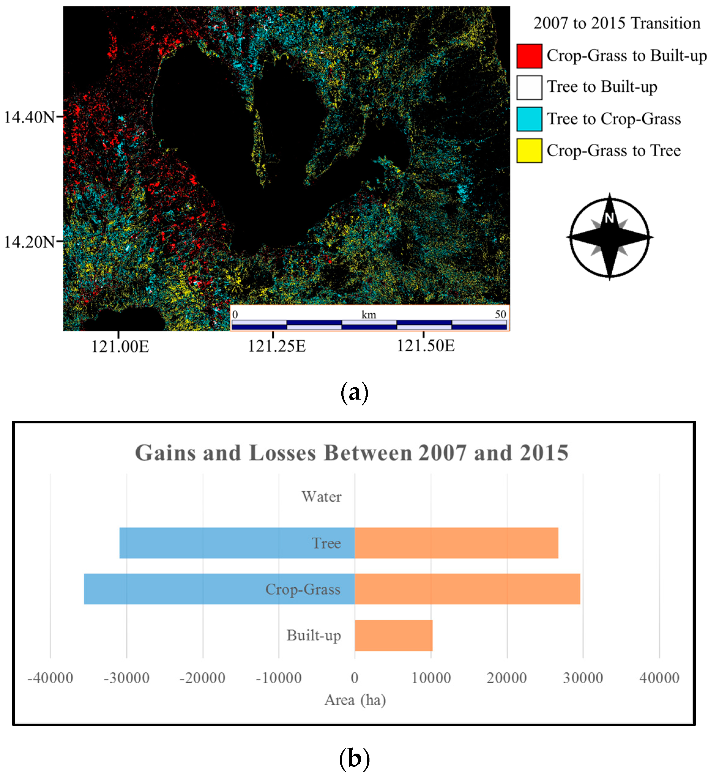
By using the Cross-Tabulation module, the transitions of each class from 2007 to 2015 were computed, as shown in Figure 3a. The gains and the losses for each LULC type, in ha, are also shown in Figure 3b. The transition map confirmed that the majority of changes in the Built-Up class are attributed to decreases in the Crop-Grass area, although a significant number of Trees areas are expected to become Built-Up land outside the protected forest areas.
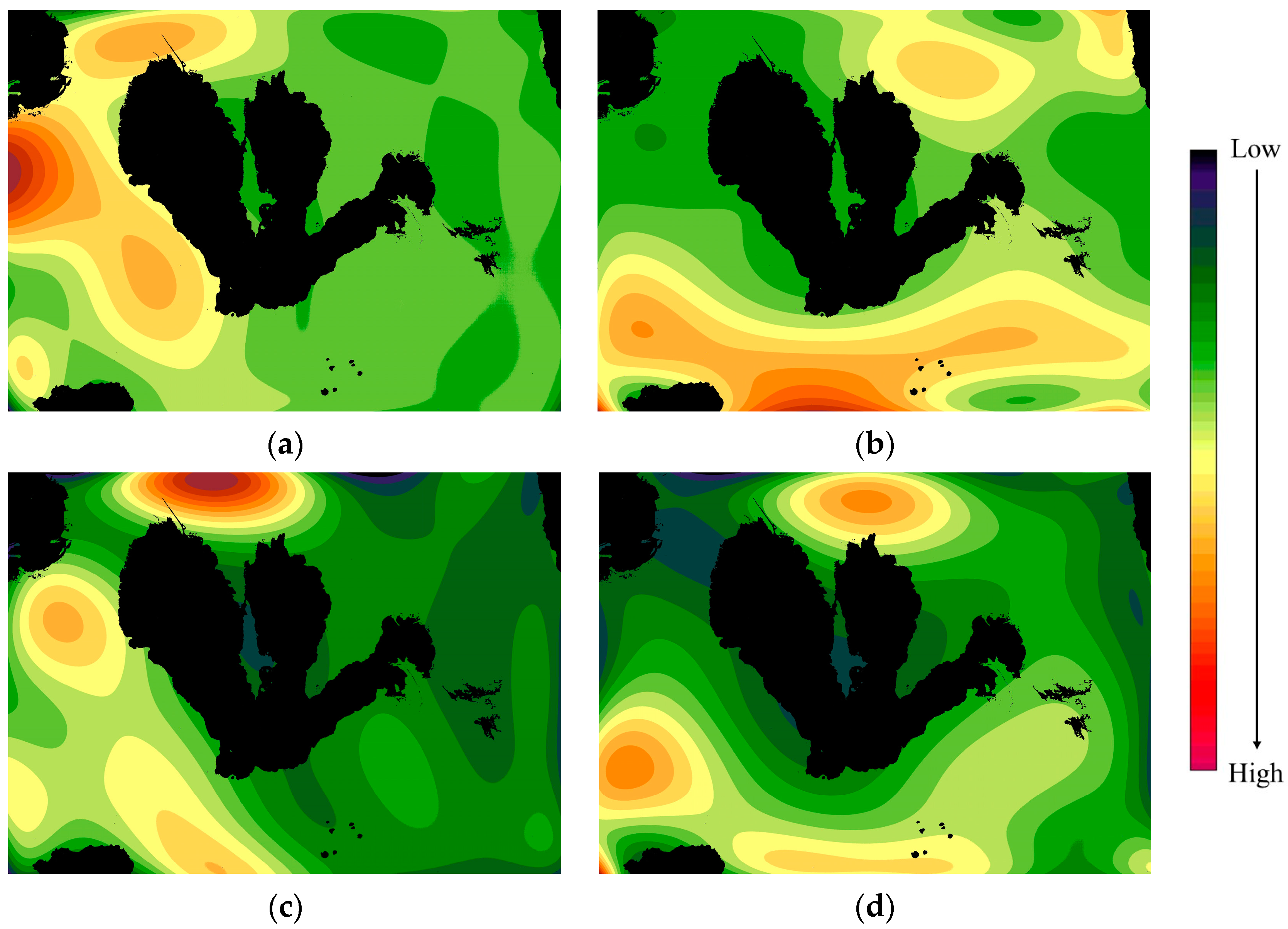
For a visual understanding of the change patterns, Figure 4 shows the spatial variation of the different LULC transition trends. The spatial change pattern of the surface was created by coding areas of change with 1 and areas of no change with 0, while treating the values in a similar manner as that for quantitative values [64] and then interpolating them by using a 9th polynomial order function. The transition trend map is shown for each class transitioning to another including Crop-Grass to Built-Up, Trees to Built-Up, Trees to Crop-Grass, and Crop-Grass to Trees. This method enables identification and understanding of the spatial trends of the transition, which can provide a better comprehension of the sites of different changes at different spatial locations. The assumption shows the change patterns that occurred in the area from 2007 to 2015. For the Built-Up class, significant changes were detected from north to south along the west side of the Laguna de Bay. High probabilities of transition were detected from the Trees (Crop-Grass) class to Built-Up class north (west) of the center of the study area. The trends for the Trees class changing into Crop-Grass were most dominant north of the center of the study area, followed secondly by the southwest area and thirdly by the south to southeast area. The largest changes were recognized at the southwestern side; however, smaller but important signs were detected at different parts of the surrounding environment, which possibly has relationships with the smaller cities located nearby. The changes of Crop-Grass to Trees were located mostly at the southern side of the study area, which is near protected areas. Thus, the Grass-Shrub-type LC is slowly changing into denser and taller vegetation due to the absence of effects from human activities.
4.2. LULC Modeling
4.2.1. Potential Explanatory Power of Driver Variables
Table 3 shows the driver variables selected for modeling of the transition potential. Each variable has a potential explanatory power that describes the strength of its relationship to the actual transition of the classes and is computed by contingency table analysis. V takes values from 0 to 1. Values near 0 show little association between variables, whereas those near 1 indicate strong association. A value of about 0.15 contains little information for explanation; more than 0.4 is considered to be a good variable [64]. Only the final variables selected for the model are listed in the table. The selection criteria was that a variable had either (i) an overall V value greater than 0.3 or (ii) V values greater than 0.15 for all of the individual LULC classes. For example, although for Dist_Protect the overall V value is below 0.3, each class shows values above 0.15.
Table 4 shows the priority of the drivers compared with other variables, showing which are the most and least influential. Table 4 (a) to (d) show the accuracy and rankings of each variable that has the largest effect on the skill of the model for (a) Crop-Grass to Built-Up; (b) Crop-Grass to Trees; (c) Trees to Built-Up; and (d) Trees to Crop-Grass. The accuracy is based on the results of the 5,000 testing pixels. The most (least) influential variable for model (a) was NL_2015 (BIO12). For model (b), the most (least) influential was DEM (NL_2015). For model (c), the most (least) influential was Pop_2007 (Road_Dist2). For model (d), the most (least) influential was Slope (NL_ch). The accuracy of each transition model in explaining its overall power for detecting the correct changes are Crop-Grass to Built-Up, 74.21%; Crop-Grass to Trees, 70.37%; Trees to Built-Up, 90.91%; and Trees to Crop-Grass, 74.31%.
4.2.2. LULC Change Modeling and its Landscape
For visual interpretation of the dynamic changes in LULC classes for each stage of the modeling (each year of 2016–2030), Video S1 is provided in the supplementary material (for business-as-usual scenario). Here, we discuss only the beginning (2015), middle (2023), and end (2030) years of the LULC map. Figure 5 shows that changes occurred from the modeling at the Laguna de Bay region. A few significant characteristic trends of change depending on each LULC class can be identified. For the Built-Up classes, the first large change is the expansion of urban areas spreading more southward and expansion at the west side of the Laguna de Bay. This type of trend has occurred in the past. Google Earth images from the 1980s in those regions [68] show strong evidence of rapid LULC change in the southern part of Metro Manila and at the west side of the Laguna de Bay. Built-Up areas have expanded in the southwestern part of the study area near a smaller lake and show development along road infrastructures at the east side of this lake. At the east side of the Laguna de Bay, significantly fewer LULC changes have occurred compared with the west side because the east side of the lake consists mainly of rural areas with low population density and less infrastructure that are thus not affected by rapid development.
For the Crop-Grass class, the main changes were detected in three areas. The first includes changes along with the development of Built-Up areas at the west side of Laguna de Bay. In addition, the Crop-Grass class area has expanded and has ensured a considerable amount of area by invading the Trees class. The second site is at the east coast of the Laguna de Bay, where Built-Up areas have not changed significantly, although the Crop-Grass class has again ensured its area by invading large amounts of Trees class areas. The third location is at the center north of the Laguna de Bay, where a similar trend of Crop-Grass invading the Trees class was noted. Future scenarios can change depending on whether countermeasures for protecting the forests were planned and implemented. Similar to using the protected areas as constraining images for unchanges, probability maps for specific regions can be applied to reduce the transition probabilities of those areas. These types of planning scenarios for the forested areas can be considered a strong decision tool for planning REDD+ (Reducing Emissions from Deforestation and forest Degradation in developing countries) actions [69] because total changes in forests can be easily calculated quantitatively, enabling sound estimation of the CO2 uptakes in those regions.
For the Trees class, the mountainous area at the east side of the Laguna de Bay and the protected areas show increments of Trees Class transition from the Crop-Grass. This occurrence depends on the ages of the people living in those rural areas, which have higher elevations and rugged terrain. When the residents become older, the land becomes more difficult to access. Agricultural lands would then begin to change into abandoned areas; thus, the trend in Crop-Grass LULC type would decrease. Other possible factors include the impact of the National Greening Program of the government [70]. In other regions, the majority of the Trees class trend shows a decrease in total area owing to its transition to the Built-Up and Crop-Grass classes.
4.2.3. LULC Change Statistics
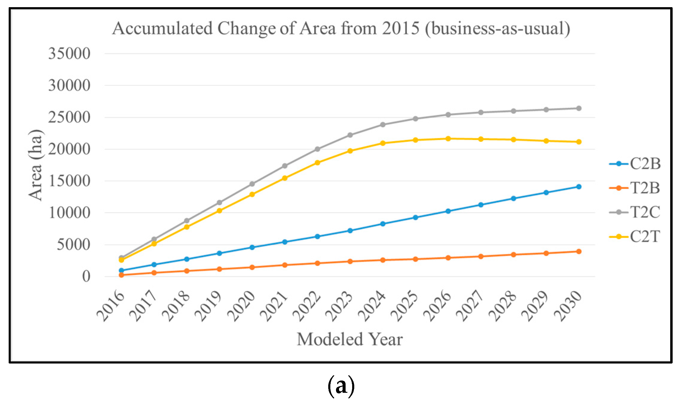
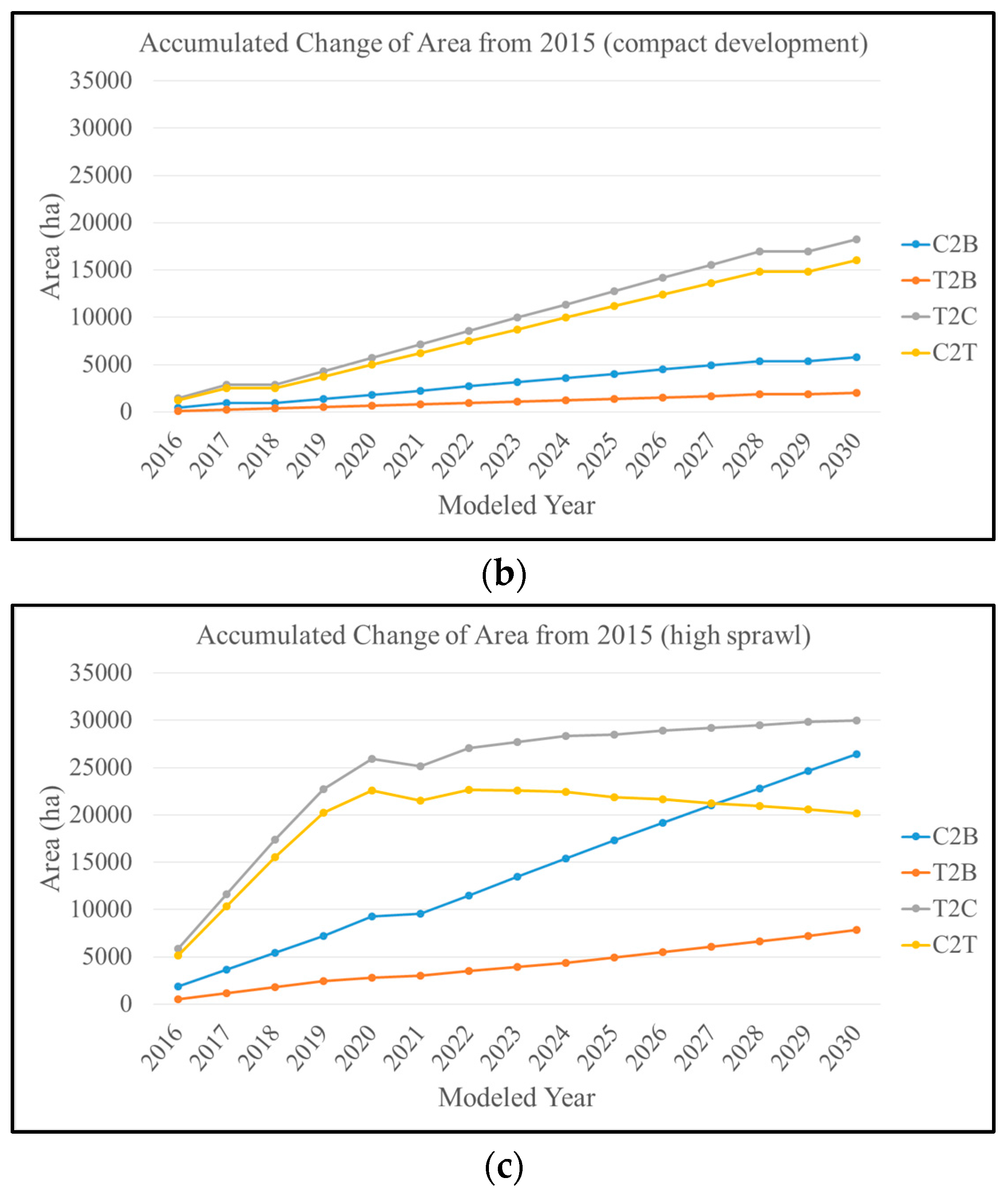
Figure 6 shows the accumulated increase in land area of each transition class from the starting year of 2015 to 2030 in yearly increments for the business-as-usual scenario, compact development scenario, and high sprawl scenario. In the business-as-usual scenario, most of the LULC change classes showed increases in total area and different growing rates; however, the Crop-Grass to Trees class showed a decrease in area beginning in 2026. The Trees to Crop-Grass and Crop-Grass to Trees classes showed a polynomial-like increase, resulting in increases of 26,409 ha and 21,166 ha, respectively, in 2030. The Crop-Grass to Built-Up and Trees to Built-Up classes showed a linear increase of land area, resulting in increases of 14,137 ha and 3946 ha, respectively, in 2030. These changes are limited to the study area. More meaningful values might be extracted when areas are divided according to administrative boundaries. In-depth information on the LULC changes for each municipal boundary is given in Spreadsheet S1 in the supplementary material. For the compact development scenario, all of the classes show a linear-like increase compared to the business-as-usual scenario. The Trees to Crop-Grass and Crop-Grass to Trees classes shows increases of 18,274 and 16,036 ha respectively, which is about 70% of the business-as-usual scenario changes. The Crop-Grass to Built-up and Trees to Built-up showed 5783 and 2000 ha increases, indicating slightly less than 50% of their areas modeled in the business-as-usual scenario. These values are similar to the modeled 2021 LULC in the business-as-usual scenario. The high sprawl scenario shows a similar pattern to the business-as-usual scenario but with a steeper increase and faster point of decrease in increments for the Crop-Grass to Trees class. The Trees to Crop-Grass and Crop-Grass to Trees classes show increases of 30,021 and 20,182 ha, respectively. The former class shows a 113% increase, but the latter remains at 95% of that of the business-as-usual scenario, showing that more Crop-Grass conversions are occurring. Crop-Grass to Built-up and Trees to Built-up classes also show an increase compared to business-as-usual scenario (26,446 and 7836 ha respectively, approximate double the area of business-as-usual scenario).
4.3. 2007–2010 Model Validation
Firstly, FoM was carried out by computing hits, misses, and false alarms between the modeled and reference LULC maps of the year 2015. The total number of pixels with hits, misses, and false alarms was 517,671, 642,064, and 964,127 respectively, resulting in a FoM of 24.37%. Secondly, Kappa statistics were computed using the modeled and reference LULC maps. The calculated Kappa statistics were: Kstandard = 0.5825; Kno = 0.6620; and Klocation = 0.6217. A Kappa value of 1 indicates total agreement and 0 indicates totally by chance. This can be interpreted as for example using the Kstandard value that the modeled 2015 map is 58% better than a chance agreement.
5. Discussion
5.1. Influences of Driver Variables Overview
Generally, the topographical drivers such as DEM and SLOPE influenced the LULC transitions for all classes. As expected, areas of higher elevations and areas with steep slopes tended to experience higher rates of transition to trees, while lower and flatter areas were more likely to convert from tree-covered areas to built-up or agricultural lands. Context drivers showed a strong influence for all LULC change classes other than the Crop-Grass to Built-up class, with the Dist_Canal variable being the top candidate for the other three transition classes. These transitions were thus affected by water availability. Road infrastructure has shown also importance (and also road type), which is logical because they are highly related to people’s mobility. The nightlight and population data showed a straightforward result of influencing changes to Built-up land. For example, Crop-Grass to Built-up transitions occurred more frequently in areas with higher populations, while Trees to Built-up transitions occurred more frequently in lower populated areas. Biophysical drivers (climatic variables) did not show as much influence as expected, although some relations were shown for variables such as BIO15 (precipitation seasonality). Our primary expectation was that LULC changes to Crop-Grass might have some relationship with climate, but this was not the case in our study (the slope and population of the nearby area were much more significant drivers).
5.2. Scenarios of the Future
Comparing the three different scenarios of future changes that we modeled in this study, although the locations of the transitions did not change significantly (because all three scenarios were based on the same transition model), the quantity and rate of LULC changes differed. If we look at the compact development scenario, where the transition rate is half of business-as-usual scenario, the conversion to Built-up in 2030 does not catch up even to that of 2022 in the business-as-usual scenario. On the other hand, if we double the rate, the development of built-up area would be mostly completed at 2023 compared to 2030 for the business-as-usual scenario. Studies on the potential impacts of these development scenarios on the local environment are still under progress, although we have concerns related to crop production, biodiversity loss (including losses of patches and corridors for wildlife), changes in local climate due to increasing heat fluxes, flood vulnerability, and river and lake water quality. A work by Wijesekara et al. [71] shows good practice of how modeling results can be used as decision/planning tools.
To achieve higher accuracy for the modeling results, two possible factors can be investigated; improving the accuracy of the LULC change map of the region and/or incorporating the zoning policies and development plans of the local governments into the modeling process. The development plans can help determine better scenarios and model areas with higher chances for transitions and the manner of development. A limitation of future modeling, especially using Markov Chains that possess stationary distribution, is that the development rate is considered from past evidence of the changes. If this rate remains constant, the trend is closer to actual trend of future change. However, past information does not always explain future modeling, meaning this can vary depending on decisions by the government or local authorities.
5.3. Other Relating Works
In this section, we compare the results of our study with those of other similar studies. First of all, how does our LULC change modeling accuracy compare to that of other similar studies? As stated in the results section, the FoM was calculated in our study as 24.37%. If we look at other similar studies for comparison, the FoM values range from 1% to 59% depending on the spatial resolution, spatial extent, and number of LULC classes mapped [40]. To compare with our study, the Twin Cities or Detroit case [40] would be the most appropriate, as these studies used maps with a similar spatial resolution, number of pixels, and number of LULC classes to our study. These two studies had FoM values of 11% and 15% respectively; slightly lower than our FoM, even though we included one additional LULC class. The studies with much higher FoM values typically had access to site-specific driver variable information (local land allocation plans) and/or aggregated modeling results to coarser spatial resolutions (i.e., larger pixel sizes) to reduce the number of locational errors [40]. Although the LULC models implemented differ among studies and have different reference characteristics, this kind of comparison can give a general idea of the modeling accuracy of our study.
Comparing our study to others that used the same MLP Markov Chain modeling method that we used [32,34,35,36,37,38,72], we can find a few important aspects for discussion. One is that many previous studies did not provide reasoning for why certain driver variables were considered or discuss why certain factors were heavily influencing different types of LULC conversions. Although the number and types of driver variables investigated differ among studies, the level of importance of each variable and the reasons why the variable is affecting LULC changes also likely varies due to different social demands and issues in each study area. By understanding the factors driving LULC conversions, local governments can have a better idea of the issues that region that is facing. We addressed this in our study by first hypothesizing why each variable may be relevant and then by measuring the influence of each variable and discussing why certain variables were relevant for different types of LULC transitions. A second point that we would like to discuss is related to model behavior. Olmedo et al. [36] showed an important aspect of changes, which could not be simulated due to the acceleration of changes that occurred in the reference year, which did not show during the calibration time period. The MLP method is a stationary model, so it is determined that it will keep the same transition rate. This means, if the development scenario changes in the future, it could either increase or decrease its changing rates, resulting in an inaccurate projection. This issue is one reason why we simulated three scenarios of the future LULC in our study area. However, most other works only simulate one future scenario. Due to this model behavior issue and also to provide useful options to government agencies in the area, we recommend considering at least a few different scenarios in addition to the business-as-usual scenario. A third point we would like to emphasize is that there should be some general consensus for presenting model validation results. For instance, one issue with Kappa and other traditional LULC accuracy metrics is that they typically give high accuracy values in study areas with few LULC changes and much lower accuracy values in areas with many LULC changes [37,38]. On the other hand, because the FoM is a ratio metric, it is unaffected by the quantity of LULC changes, so it is a good practice to also report FoM in LULC change modeling studies (as we have done in this study).
5.4. Accomplished Tasks and Future Works
This work follows similar processes to other MLP Markov Chain studies to model the future landscape of Laguna de Bay. Using Landsat and SAR images, a spatial resolution of 25 m was achieved, showing finer information compared to using Landsat data alone. Developing LULC maps in tropical regions such as the Philippines, Indonesia, or other Southeast Asian countries is a difficult task due to frequent cloud cover (which obstructs the view of the land surface for optical satellite images). Therefore utilizing SAR data was an advantage in developing the historical LULC change data. We have worked on finding the characteristics of the changing pattern and compared these with other related studies. The 27 variables we considered was an enormous amount, around double the number of variables from the study that showed the highest number (14 drivers [72]). We have found explainable relations with the drivers used, and the study gave a clear idea of how LULC is likely developing in this area. Although we did use a large number of driver variables, we could not take into account the local zoning policies of the cities and towns in the study area (due to a lack of data availability), which also have a significant effect on LULC change. It is a very time-consuming and challenging task to visit all of the municipalities in the area to collect (and possibly digitize) their zoning and development plans, but this would probably further enhance the modeling results.
We found that urban sprawl, which was the focus of this study, is expected to continue occurring throughout the future timeframe that we considered (2016–2030). Looking at the surrounding area as a continuous landscape, we were concerned especially with how the existing agricultural and forested lands could be maintained in the future. We plan to continue the work to present a scientific standard for how these lands should be preserved according to various social-environmental impacts, which could be caused by the future LULC changes.
6. Conclusions
The objectives of this study were to model and map the future LULC of the Laguna de Bay area of the Philippines, which has a significant impact on the lake’s water quantity and water quality. The study area is significant mainly because of the importance of the lake to the population of Metro Manila and the surrounding cities and towns. The future LULC was modeled and mapped by using Markov Chain analysis, and the transition probabilities were calculated by using historical LULC change data and freely available data related to the drivers of the LULC changes such as demographic, economic, topographic, infrastructure, and climate variables. Three questions are addressed in this work: (1) Where are different LULC changes taking place?; (2) What are the variables that best explain the changes (e.g., what are the drivers)?; and (3) What is the rate at which these changes are likely to take place? The major LULC changes in the area included an increase in Built-Up areas at the west side of the Laguna de Bay, south of Metro Manila, and changes of many areas between the Crop-Grass and Trees classes, owing to logging, cropland abandonment, reforestation, and other factors. In total, approximately 7800 to 44,000 ha of land within the study area are modeled to be converted to the Built-Up class by 2030, depending on the development scenario. We tested three scenarios: ‘business-as-usual’, ‘compact development’, and ‘high urban sprawl’. The study has shown the extent of the changed areas in addition to the patterns and the locations of these future changes and identified the variables considered to be significant drivers of these changes (which varied for different types of LULC transitions). This information can be used by decision makers in deciding the necessary actions for preventing issues that might arise if such developments occur. The increase in Built-Up areas can affect local environmental factors such as temperature, local climatic conditions, and ecological effects [73,74]. These issues could also directly affect biodiversity and health by leading to an increase in the number of mosquitos carrying malaria and dengue fever [75,76]. Flooding is likely to become more frequent owing to the increase in urban areas; therefore, more strategic measures need to be developed to mitigate the impacts. The method implemented in this study can be used as a tool for making more informed decisions. Future work will assess the environmental impacts from future changes in the urban environments according to the various scenarios of development.
Supplementary Materials
The following are available online at www.mdpi.com/2073-445X/6/2/26/s1. Figure S1: Interpretation of all driver variables included in the model. (a) BIO3; (b) BIO6; (c) BIO7; (d) BIO12; (e) BIO15; (f) BIO19; (g) DEM; (h) SLOPE; (i) Dist_Built; (j); Dist_Crop; (k) Dist_Tree; (l) Dist_Water; (m) Road_Dist1; (n) Road_Dist2; (o) Road_Dist3; (p) Road_Dist4; (q) Dist_River; (r) Dist_Canal; (s) Dist_Stream; (t) Dist_Golf; (u) Dist_Protect; (v) Pop_2007; (w) Pop_2015; (x) Pop_Ch; (y) NL_2007; (z) NL_2015; (A) NL_Ch; Spreadsheet S1: Each LULC class total area (hectare) within each municipal boundaries for the ‘business-as-usual’, ‘compact development’, and ‘high urban sprawl’ scenarios; Video S1: LULC dynamics for Laguna de Bay region 2016–2030.
Author Contributions
K.I. designed, collected, and analyzed the data and took the lead in writing this article. B.A.J. collected and analyzed the data and edited the manuscript. A.O., D.B.M.-M., I.E., and M.B. gave critical information and revisions to this manuscript in all sections to improve in the quality of the work.
Conflicts of Interest
The authors declare no conflict of interest.
References
- World Urbanization Prospects: The 2014 Revision (ST/ESA/SER.A/352); Population Division, Department of Economic and Social Affairs, United Nations: New York, NY, USA, 2015.
- Taubenböck, H.; Esch, T.; Felbier, A.; Wiesner, M.; Roth, A.; Dech, S. Monitoring urbanization in mega cities from space. Remote Sens. Environ. 2012, 117, 162–176. [Google Scholar] [CrossRef]
- Gill, S.E.; Handley, J.F.; Ennos, A.R.; Pauleit, S. Adapting Cities for Climate Change: The Role of the Green Infrastructure. Built Environ. 2007, 33, 115–133. [Google Scholar] [CrossRef]
- Satterthwaite, D.; McGranahan, G.; Tacoli, C. Urbanization and its implications for food and farming. Philos. Trans. R. Soc. B 2010, 365, 2809–2820. [Google Scholar] [CrossRef] [PubMed]
- Oliver, T.H.; Morecroft, M.D. Interactions between climate change and land use change on biodiversity: Attribution problems, risks, and opportunities. WIREs Clim. Chang. 2014, 5, 317–335. [Google Scholar] [CrossRef]
- Edelman, D.J. Managing the Urban Environment of Manila. Adv. Appl. Sociol. 2016, 6, 101–133. [Google Scholar] [CrossRef]
- Bürgi, M.; Hersperger, A.M.; Schneeberger, N. Driving forces of landscape change—Current and new directions. Landsc. Ecol. 2004, 19, 857–868. [Google Scholar] [CrossRef]
- Figueroa, F.; Sánchez–Cordero, V.; Meave, J.A.; Trejo, I. Socioeconomic context of land use and land cover change in Mexican biosphere reserves. Environ. Conserv. 2009, 36, 180–191. [Google Scholar] [CrossRef]
- Kolb, M.; Mas, J.F.; Galicia, L. Evaluating drivers and transition potential models in a complex landscape in southern Mexico. Int. J. Geogr. Inf. Sci. 2013, 27, 1804–1827. [Google Scholar] [CrossRef]
- Seto, K.; Güneralp, B.; Hutyra, L. Global forecasts of urban expansion to 2030 and direct impacts on biodiversity and carbon pools. Proc. Natl. Acad. Sci. USA 2012, 109, 16083–16088. [Google Scholar] [CrossRef] [PubMed]
- Han, H.; Yang, C.; Song, J. Scenario Simulation and the Prediction of Land Use and Land Cover Change in Beijing, China. Sustainability 2015, 7, 4260–4279. [Google Scholar] [CrossRef]
- Pitman, A.J.; de Noblet-Ducoudré, N.; Avila, F.B.; Alexander, L.V.; Boisier, J.-P.; Brovkin, V.; Delire, C.; Cruz, F.; Donat, M.G.; Gayler, V.; et al. Effects of land cover change on temperature and rainfall extremes in multi-model ensemble simulations. Earth Syst. Dyn. 2012, 3, 213–231. [Google Scholar]
- Lasco, R.D.; Pulhin, F.B. Forest land use change in the Philippines and climate change mitigation. Mitig. Adapt. Strateg. Glob. Chang. 2000, 5, 81–97. [Google Scholar] [CrossRef]
- Malaque, I.R.; Yokohari, M. Urbanization process and the changing agricultural landscape pattern in the urban fringe of Metro Manila, Philippines. Environ. Urban 2007, 19, 191–206. [Google Scholar] [CrossRef]
- Murakami, A.; Palijon, A.M. Urban Sprawl and Land Use Characteristics in the Urban Fringe of Metro Manila, Philippines. J. Asian Archit. Build. Eng. 2005, 1, 177–183. [Google Scholar] [CrossRef]
- Alexandratos, N.; Bruinsma, J. World Agriculture towards 2030/2050: The 2012 Revision; ESA Working Paper No. 12-03; FAO: Rome, Italy, 2012. [Google Scholar]
- Perry, D.A.; Oren, R.; Hart, S.C. Forest Ecosystems, 2nd ed.; The Johns Hopkins University Press: Baltimore, MD, USA, 2008. [Google Scholar]
- Rola, A.C.; Sajise, J.A.U.; Harder, D.; Alpuerto, J.M. Soil conservation decision and upland corn productivity: A Philippine case study. Asian J. Agric. Dev. 2009, 6, 1–19. [Google Scholar]
- Briones, R.U.; Ella, V.B.; Bantayan, N.C. Hydrologic Impact Evaluation of Land Use and Land Cover Change in Palico Watershed, Batangas, Philippines Using the SWAT Model. J. Environ. Sci. Manag. 2016, 19, 96–107. [Google Scholar]
- Tongson, E.E.; Faraon, A.A. Hydrologic Atlas of Laguna de Bay 2012; Laguna Lake Development Authority and WWF-Philippines: Quezon City, Philippines, 2012. [Google Scholar]
- Murayama, Y.; Estoque, R.C.; Subasinghe, S.; Hou, H.; Gong, H. Land-Use/Land-Cover Changes in Major Asian and African Cities. Ann. Rep. Multi Use Soc. Econ. Data Bank 2015, 92, 11–58. [Google Scholar]
- Boori, M.S.; Choudhary, K.; Kupriyanov, A.; Kovelskiy, V. Satellite data for Singapore, Manila and Kuala Lumpur city growth analysis. Data Brief. 2016, 7, 1576–1583. [Google Scholar] [CrossRef] [PubMed]
- Abino, A.C.; Kim, S.Y.; Jang, M.N.; Lee, Y.J.; Chung, J.S. Assessing land use and land cover of the Marikina sub-watershed, Philippines. Forest Sci. Technol. 2015, 11, 65–75. [Google Scholar] [CrossRef]
- Global Footprint Network. Ecological Footprint Report: Restoring Balance in Laguna Lake Region; Global Footprint Network: Oakland, CA, USA, 2013. [Google Scholar]
- Wealth Accounting and the Valuation of Ecosystem Services (WAVES). Ecosystem Accounts Inform Policies for Better Resource Management of Laguna de Bay. Available online: https://www.wavespartnership.org/en/knowledge-center/ecosystem-accounts-inform-policies-better-resource-management-laguna-de-bay (accessed on 20 March 2017).
- Rañola, R.F., Jr.; Rañola, F.M.; Casin, C.S.; Tan, M.F.O. LakeHEAD Progress Report: The Social and Economic Basis for Managing Environmental Risk for Sustainable Food and Health in Watershed Planning: The Case of Silang-Sta; Rosa Sub-Watershed Communities in Lake Laguna Region; Research Institute for Humanity and Nature: Kyoto, Japan, 2010–2011. [Google Scholar]
- Mishra, V.N.; Rai, P.K.; Mohan, K. Prediction of land use changes based on land change modeler (LCM) using remote sensing: A case study of Muzaffarpur (Bihar), India. J. Geogr. Inst. Jovan Cvijic 2014, 64, 111–127. [Google Scholar] [CrossRef]
- Fathizad, H.; Rostami, N.; Faramarzi, M. Detection and prediction of land cover changes using Markov chain model in semi-arid rangeland in western Iran. Environ. Monit. Assess. 2015, 187, 629. [Google Scholar] [CrossRef] [PubMed]
- Megahed, Y.; Cabral, P.; Silva, J.; and Caetano, M. Land Cover Mapping Analysis and Urban Growth Modelling Using Remote Sensing Techniques in Greater Cairo Region—Egypt. ISPRS Int. J. Geo Inf. 2015, 4, 1750–1769. [Google Scholar] [CrossRef]
- Agarwal, C.; Green, G.M.; Grove, J.M.; Evans, T.P.; Schweik, C.M. A Review and Assessment of Land-Use Change Models Dynamics of Space, Time, and Human Choice; U.S. Dept. of Agriculture: Quilcene, WA, USA; Forest Service: Washington, DC, USA; Northeastern Research Station: Newtown Square, PA, USA, 2002.
- National Research Council. Advancing Land Change Modeling: Opportunities and Research Requirements. Chapter: 2 Land Change Modeling Approaches; The National Academies Press: Washington, DC, USA, 2014. [Google Scholar]
- Triantakonstantis, D.; Stathakis, D. Urban growth prediction in Athens, Greece, using Artificial Neural Networks. Int. J. Civil Environ. Struct. Construct. Archit. Eng. 2015, 9, 234–238. [Google Scholar]
- Grekousis, G.; Manetos, P.; Photis, Y.N. Modeling urban evolution using neural networks, fuzzy logic and GIS: The case of the Athens metropolitan area. Cities 2013, 30, 193–203. [Google Scholar] [CrossRef]
- Zhai, R.; Zhang, C.; Li, W.; Boyer, M.A.; Hanink, D. Prediction of Land Use Change in Long Island Sound Watersheds Using Nighttime Light Data. Land 2016, 5, 44. [Google Scholar] [CrossRef]
- Ahmed, B.; Ahmed, R. Modeling Urban Land Cover Growth Dynamics Using Multi-Temporal Satellite Images: A Case Study of Dhaka, Bangladesh. ISPRS Int. J. Geo Inf. 2012, 1, 3–31. [Google Scholar] [CrossRef]
- Olmedo, M.T.C.; Pontius, R.G., Jr.; Paegelow, M.; Mas, J.-M. Comparison of simulation models in terms of quantity and allocation of land change. Environ. Model. Softw. 2015, 69, 214–221. [Google Scholar] [CrossRef]
- Riccioli, F.; El Asmar, T.; El Asmar, J.P.; Fagarazzi, C.; Casini, L. Artificial neural network for multifunctional areas. Environ. Monit. Assess. 2016, 188, 67. [Google Scholar] [CrossRef] [PubMed]
- Wang, W.; Zhang, C.; Allen, J.M.; Li, W.; Boyer, M.A.; Segerson, K.; Silander, J.A. Analysis and Prediction of Land Use Changes Related to Invasive Species and Major Driving Forces in the State of Connecticut. Land 2016, 5, 25. [Google Scholar] [CrossRef]
- Chaudhuri, G.; Clarke, K. The SLEUTH and land use change model: A review. Environ. Resour. Res. 2013, 1, 88–105. [Google Scholar]
- Pontius Jr, R.G.; Boersma, W.; Castella, J.-C.; Clarke, K.; de Nijs, T.; Dietzel, C.; Duan, Z.; Fotsing, E.; Goldstein, N.; Kok, K.; et al. Comparing the input, output, and validation maps for several models of land change. Ann. Reg. Sci. 2008, 42, 11–47. [Google Scholar] [CrossRef]
- Clark Labs. TerrSet Geospatial Monitoring and Modeling Software; Clark Labs, Clark University: Worcester, MA, USA, 2015. [Google Scholar]
- Laguna Lake Development Authority, Water Quality Report: Laguna de Bay and Its Tributaries. Available online: http://www.llda.gov.ph/index.php?option=com_content&view=article&id=218&Itemid=679 (accessed on 20 March 2017).
- Google Earth, V 7.1.8.3036. (24 March 2016), Laguna de Bay, Philippines, 14.340535°N, 121.241762°E, Eye alt 62.90 km. DigitalGlobe 2016, Google 2016, CNES/Astrium 2016. Available online: http://www.earth.google.com (accessed on 20 March 2017).
- Johnson, B.A.; Iizuka, K.; Bragais, M.; Endo, I.; Magcale-Macandog, D. Employing crowdsourced geographic data and multi-temporal/multi-sensor satellite imagery to monitor land cover change: A case study in an urbanizing region of the Philippines. Comput. Environ. Urban Syst. 2017, 64, 184–193. [Google Scholar] [CrossRef]
- Lambin, E.F.; Turner, B.L.; Geist, H.J.; Agbola, S.B.; Angelsen, A.; Bruce, J.W.; Coomes, O.T.; Dirzo, R.; Fischer, G.; Folke, C.; et al. The causes of land-use and land-cover change: Moving beyond the myths. Glob. Environ. Chang. 2001, 11, 261–269. [Google Scholar] [CrossRef]
- Lambin, E.F.; Geist, H.J.; Lepers, E. Dynamics of land-use and land-cover change in tropical regions. Annu. Rev. Environ Resour. 2003, 28, 205–241. [Google Scholar] [CrossRef]
- PhilGIS—Philippines GIS Data Clearinghouse. Available online: https://www.philgis.org/ (accessed on 20 March 2017).
- EarthExplorer (USGS). Available online: https://earthexplorer.usgs.gov/ (accessed on 20 March 2017).
- OpenStreetMap—GEOFABRIK Downloads. Available online: http://download.geofabrik.de/asia/philippines.html (accessed on 3 March 2016 ).
- NOAA Earth Observtion Group (EOG). Available online: https://ngdc.noaa.gov/eog/ (accessed on 20 March 2017).
- WorldPop. Available online: http://www.worldpop.org.uk/ (accessed on 20 March 2017).
- WorldClim—Global Climate Data. Available online: http://www.worldclim.org/ (accessed on 20 March 2017).
- Hijmans, R.J.; Cameron, S.E.; Parra, J.L.; Jones, P.G.; Jarvis, A. Very high resolution interpolated climate surfaces for global land areas. Int J Climatol. 2005, 25, 1965–1978. [Google Scholar] [CrossRef]
- O’Donnell, M.S.; Ignizio, D.A. Bioclimatic Predictors for Supporting Ecological Applications in the Conterminous United States; U.S. Geological Survey Data Series 691; U.S. Geological Survey: Reston, VA, USA, 2012.
- Van Wart, J.; van Bussel, L.G.J.; Wolf, J.; Licker, R.; Grassini, P.; Nelson, A.; Boogaard, H.; Gerber, J.; Mueller, N.D.; Claessens, L.; et al. Use of agro-climatic zones to upscale simulated crop yield potential. Field Crops Res. 2013, 143, 44–55. [Google Scholar] [CrossRef]
- Kim, I.; Le, Q.B.; Park, S.J.; Tenhunen, J.; Koellner, T. Driving Forces in Archetypical Land-Use Changes in a Mountainous Watershed in East Asia. Land 2014, 3, 957–980. [Google Scholar] [CrossRef]
- Ruan, X.; Qiu, F.; Dyck, M. The effects of environmental and socioeconomic factors on land-use changes: A study of Alberta, Canada. Environ. Monit. Assess. 2016, 188, 446. [Google Scholar] [CrossRef] [PubMed]
- Mellander, C.; Lobo, J.; Stolarick, K.; Matheson, Z. Night-Time Light Data: A Good Proxy Measure for Economic Activity? PLoS ONE 2015, 10, e0139779. [Google Scholar] [CrossRef] [PubMed]
- Stathakis, D. Forecasting Urban Expansion Based on Night Lights. Int. Arch. Photogramm. Remote Sens. Spat. Inf. Sci. 2016, XLI-B8, 1049–1054. [Google Scholar] [CrossRef]
- Stevens, F.R.; Gaughan, A.E.; Linard, C.; Tatem, A.J. Disaggregating Census Data for Population Mapping Using Random Forests with Remotely-Sensed and Ancillary Data. PLoS ONE 2015, 10, e0107042. [Google Scholar] [CrossRef] [PubMed]
- Linard, C.; Gilbert, M.; Snow, R.W.; Noor, A.M.; Tatem, A.J. Population Distribution, Settlement Patterns and Accessibility across Africa in 2010. PLoS ONE 2012, 7, e31743. [Google Scholar] [CrossRef] [PubMed]
- Mas, J.F.; Puig, H.; Palacio, J.L.; Lopez, A.S. Modelling deforestation using GIS and artificial neural networks. Environ. Model. Softw. 2004, 19, 461–471. [Google Scholar] [CrossRef]
- Yuan, H.; Van Der Wiele, C.F.; Khorram, S. An automated artificial neural network system for land use/land cover classification from Landsat TM imagery. Remote Sens. 2009, 1, 243–265. [Google Scholar] [CrossRef]
- Eastman, J.R. TerrSet Help File; Clark University: Worcester, MA, USA, 2015. [Google Scholar]
- Takada, T.; Miyamoto, A.; Hasegawa, F.S. Derivation of a yearly transition probability matrix for land-use dynamics and its applications. Landsc Ecol. 2010, 24, 561–572. [Google Scholar] [CrossRef]
- Estoque, R.C.; Murayama, Y. Corrigendum to ‘Examining the potential impact of land use/cover changes on the ecosystem services of Baguio city, the Philippines: A Scenario-based analysis’. Appl. Geogr. 2012, 35, 316–326. [Google Scholar]
- Pontius, R.G. Quantification error versus location error in comparison of categorical maps. Photogramm. Eng. Remote Sens. 2000, 66, 1011–1016. [Google Scholar]
- Google Earth, V 7.1.8.3036. (31 December 1984; 30 December 1990; 31 December 1996; 31 December 2002; 31 December 2008), Laguna de Bay, Philippines, 14.340535°N, 121.241762°E, Eye alt 62.90 km. Landsat/Copernicus. Available online: http://www.earth.google.com (accessed on 20 March 2017).
- Iizuka, K.; Tateishi, R. Estimation of CO2 Sequestration by the Forests in Japan by Discriminating Precise Tree Age Category using Remote Sensing Techniques. Remote Sens. 2015, 7, 15082–15113. [Google Scholar] [CrossRef]
- National Greening Program, Department of Environment and Natural Resrouces. Available online: http://www.denr.gov.ph/priority-programs/national-greening-program.html (accessed on 20 March 2017).
- Wijesekara, G.N.; Farjad, B.; Gupta, A.; Qiao, Y.; Delaney, P.; Marceau, D.J. A comprehensive land-use/hydrological modeling system for scenario simulations in the Elbow River Watershed, Alberta, Canada. Environ Manag. 2014, 53, 357–381. [Google Scholar] [CrossRef] [PubMed]
- Losiri, C.; Nagai, M.; Ninsawat, S.; Shrestha, R.P. Modeling Urban Expansion in Bangkok Metropolitan Region Using Demographic–Economic Data through Cellular Automata-Markov Chain and Multi-Layer Perceptron-Markov Chain Models. Sustainability 2016, 8, 686. [Google Scholar] [CrossRef]
- Dale, V. The Relationship between Land-Use Change and Climate Change. Ecol. Appl. 1997, 7, 753–769. [Google Scholar] [CrossRef]
- Zhang, Y.; Smith, J.A.; Luo, L.; Wang, Z.; Baeck, M.L. Urbanization and Rainfall Variability in the Beijing Metropolitan Region. J. Hydrometeorol. 2014, 15, 2219–2235. [Google Scholar] [CrossRef]
- Bravo, L.; Roque, V.G.; Brett, J.; Dizon, R.; L’Azou, M. Epidemiology of Dengue Disease in the Philippines (2000–2011): A Systematic Literature Review. PLoS Negl. Trop. Dis. 2014, 8, e3027. [Google Scholar] [CrossRef] [PubMed]
- Su, G. Correlation of Climatic Factors and Dengue Incidence in Metro Manila, Philippines. Ambio 2008, 37, 292–294. [Google Scholar] [CrossRef]
Figure 1.
Overview of the study area, the Laguna de Bay district, and the surrounding environment in the Philippines. Metro Manila is shown in the northwest corner. Referenced from Google Earth [43].
Figure 1.
Overview of the study area, the Laguna de Bay district, and the surrounding environment in the Philippines. Metro Manila is shown in the northwest corner. Referenced from Google Earth [43].

Figure 2.
Overall flowchart of the methodology used in this study.

Figure 3.
(a) Area of transitions occurring from 2007 to 2015 for each land-use/land-cover (LULC) type; (b) Total area of gains and losses computed within the study area for each LULC type.
Figure 3.
(a) Area of transitions occurring from 2007 to 2015 for each land-use/land-cover (LULC) type; (b) Total area of gains and losses computed within the study area for each LULC type.

Figure 4.
Patterns or trends of transition through space for (a) Crop-Grass to Built-up; (b) Crop-Grass to Trees; (c) Trees to Built-up; and (d) Trees to Crop-Grass. Red (blue) color indicates the higher (lower) chances of transition. The data contain no specific values because no mean is represented.

Figure 5.
Land-use/land-cover (LULC) modeling of the Laguna de Bay environment for (a) 2015; (b) 2023; and (c) 2030. (a–c) shows the hard classified map; (d–f) shows the percentage of each LULC class within the study area. The numbers indicated after the alphabet represent the different modeled scenarios. Thus (a-1) is the business-as-usual scenario; (a-2) is the compact development scenario; and (a-3) is the high sprawl scenario. Legends in the pie-chart correspond to the colors of the LULC class in the hard classified map.
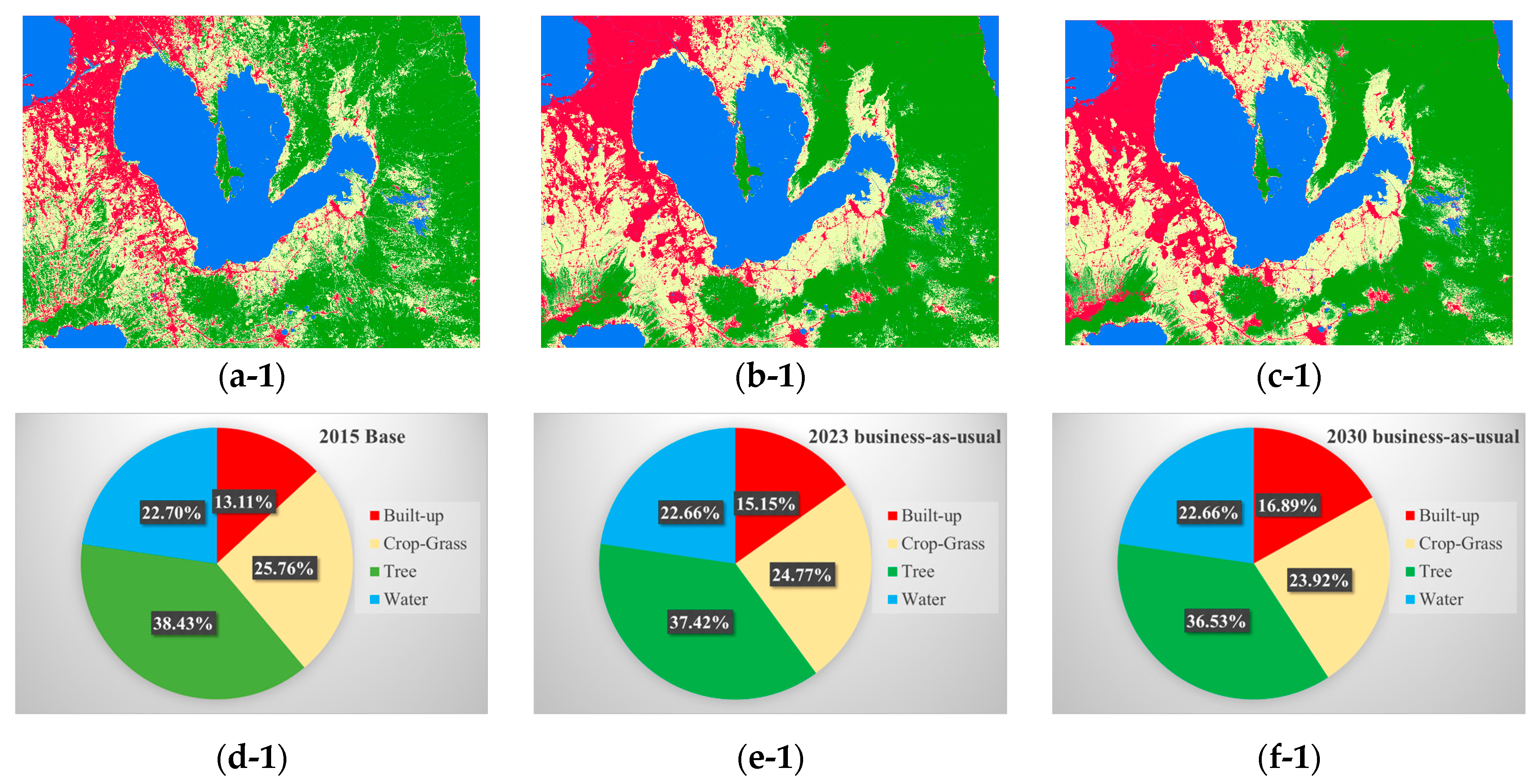
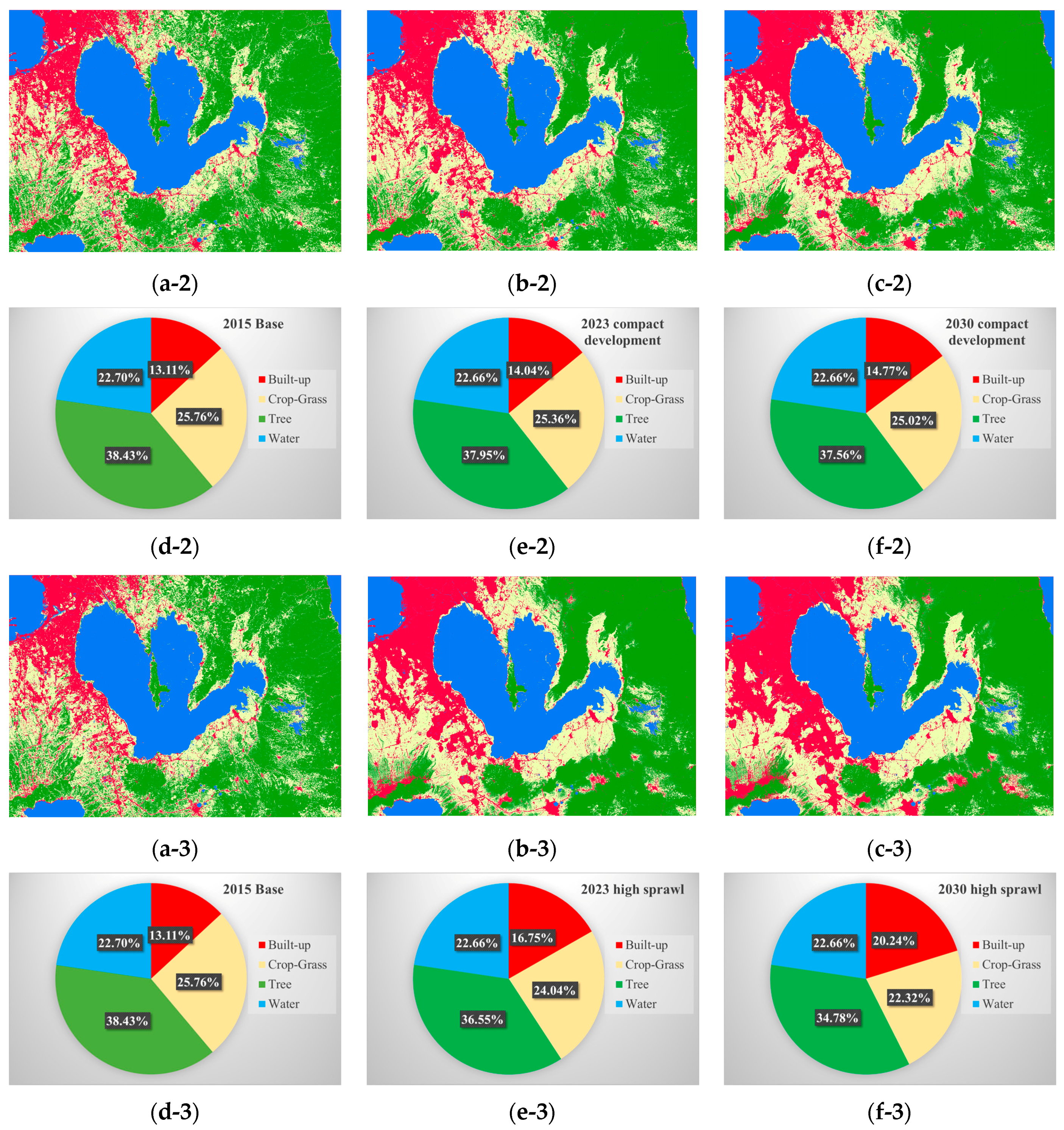
Figure 6.
Trends of LULC class and net area of increase at each stage of the modeling. The base year is 2015. C2B, Crop-Grass to Built-up; T2B, Trees to Built-up; T2C, Trees to Crop-Grass; C2T, Crop-Grass to Trees. (a) Business-as-usual scenario; (b) compact development scenario; (c) high sprawl scenario.


Table 1.
Complete list of all variables collected in this study.
| Category | Driver | Abbreviation | Unit | Year | Data Source |
|---|---|---|---|---|---|
| Climate | Annual Mean Temperature | BIO1 | °C | 1960–1990 | PhilGIS [47] |
| Mean Diurnal Range | BIO2 | ||||
| Isothermality | BIO3 | % | |||
| Temperature Seasonality | BIO4 | °C | |||
| Max. Temperature of Warmest Month | BIO5 | ||||
| Min. Temperature of Coldest Month | BIO6 | ||||
| Temperature Annual Range | BIO7 | ||||
| Mean Temperature of Wettest Quarter | BIO8 | ||||
| Mean Temperature of Driest Quarter | BIO9 | ||||
| Mean Temperature of Warmest Quarter | BIO10 | ||||
| Mean Temperature of Coldest Quarter | BIO11 | ||||
| Annual Precipitation | BIO12 | mm | |||
| Precipitation of Wettest Month | BIO13 | ||||
| Precipitation of Driest Month | BIO14 | ||||
| Precipitation Seasonality | BIO15 | % | |||
| Precipitation of Wettest Quarter | BIO16 | mm | |||
| Precipitation of Driest Quarter | BIO17 | ||||
| Precipitation of Warmest Quarter | BIO18 | ||||
| Precipitation of Coldest Quarter | BIO19 | ||||
| Topography | Elevation | DEM | m | 2000 | SRTM [48] |
| Slope | Slope | degrees | |||
| Aspect | Aspect | ||||
| Spatial Context | Distance from Built-up | Dist_Built | Lat/Long degrees | 2007 | Classified LULC 2007 |
| Distance from Crop-Grass | Dist_Crop | ||||
| Distance from Trees | Dist_Tree | ||||
| Distance from Water | Dist_Water | ||||
| Distance from Primary Road | Dist_Road1 | 3 March 2016 | OpenStreetMap [49] | ||
| Distance from Secondary Road | Dist_Road2 | ||||
| Distance from Tertiary Road | Dist_Road3 | ||||
| Distance from Other Roads | Dist_Road4 | ||||
| Distance from Canal | Dist_Canal | ||||
| Distance from River | Dist_River | ||||
| Distance from Stream | Dist_Stream | ||||
| Distance from Golf Course | Dist_Golf | 2004 | PhilGIS [47] | ||
| Distance from Protected Area | Dist_Protect | 2013 | |||
| Nightlight Data | Night Light Data 2007 | NL_2007 | DN | 2007 | NOAA Earth Observation Group [50] |
| Night Light Data 2015 | NL_2015 | nanoWatts/cm2/sr | 2015 | ||
| Night Light Change 2007 to 2015 | NL_Ch | - | |||
| Population | Population Map 2007 | Pop_2007 | People per hectare | 2007 | WorldPop [51] |
| Population Map 2015 | Pop_2015 | 2015 | |||
| Population Change 2007 to 2015 | Pop_Ch | - |
Table 2.
Markov transition probability matrix (business-as-usual scenario).
| Probability of changing to (2030): | |||||
|---|---|---|---|---|---|
| Built-Up | Crop-Grass | Trees | Water | ||
| LULC Given (2015) | Built-Up | 1.0000 | 0.0000 | 0.0000 | 0.0000 |
| Crop-Grass | 0.1137 | 0.5745 | 0.3118 | 0.0000 | |
| Trees | 0.0211 | 0.2372 | 0.7417 | 0.0000 | |
| Water | 0.0000 | 0.0000 | 0.0000 | 1.0000 | |
Table 3.
Test of the explanatory power (Cramer’s V) of each variable.
| Variable | |||||||||
|---|---|---|---|---|---|---|---|---|---|
| BIO3 | BIO6 | BIO7 | BIO12 | BIO15 | BIO19 | DEM | Slope | Dist-Built | |
| Overall | 0.3426 | 0.4680 | 0.4208 | 0.3250 | 0.4934 | 0.3757 | 0.6107 | 0.5649 | 0.3609 |
| Built-up | 0.2769 | 0.2908 | 0.2815 | 0.2803 | 0.5390 | 0.2748 | 0.4411 | 0.3142 | 0.3517 |
| Crop-Grass | 0.1242 | 0.1934 | 0.2315 | 0.1095 | 0.2223 | 0.1603 | 0.3273 | 0.3434 | 0.3583 |
| Trees | 0.4517 | 0.6166 | 0.6078 | 0.4476 | 0.6069 | 0.5680 | 0.6465 | 0.6220 | 0.2905 |
| Water | 0.4382 | 0.6450 | 0.5032 | 0.3886 | 0.5268 | 0.4256 | 0.8902 | 0.8400 | 0.4193 |
| Dist_Crop | Dist_Tree | Dist_Water | Road_Dist1 | Road_Dist2 | Road_Dist3 | Road_Dist4 | Road_River | Road_Canal | |
| Overall | 0.4469 | 0.5144 | 0.4352 | 0.3046 | 0.3767 | 0.3793 | 0.3921 | 0.3398 | 0.4165 |
| Built-Up | 0.1702 | 0.1664 | 0.2347 | 0.3634 | 0.4570 | 0.3979 | 0.3749 | 0.2757 | 0.4865 |
| Crop-Grass | 0.2912 | 0.2890 | 0.1899 | 0.2226 | 0.2815 | 0.3151 | 0.3746 | 0.2452 | 0.1678 |
| Trees | 0.2946 | 0.4073 | 0.6398 | 0.2488 | 0.3686 | 0.2974 | 0.2387 | 0.1875 | 0.5701 |
| Water | 0.7692 | 0.8848 | 0.5588 | 0.3390 | 0.3628 | 0.4630 | 0.5084 | 0.5261 | 0.3484 |
| Dist_Stream | Dist_Golf | Dist_Protect | Pop_2007 | Pop_2015 | P0p_Ch | NL_2007 | NL_2015 | NL_Ch | |
| Overall | 0.3612 | 0.3149 | 0.2484 | 0.4943 | 0.4910 | 0.5363 | 0.4659 | 0.4047 | 0.3218 |
| Built-Up | 0.3735 | 0.3941 | 0.2070 | 0.7183 | 0.7180 | 0.7132 | 0.6368 | 0.6597 | 0.4658 |
| Crop-Grass | 0.3159 | 0.1679 | 0.2147 | 0.3932 | 0.3838 | 0.4545 | 0.2989 | 0.1654 | 0.1922 |
| Trees | 0.3313 | 0.3677 | 0.2214 | 0.3731 | 0.3722 | 0.3477 | 0.5213 | 0.3142 | 0.3649 |
| Water | 0.4078 | 0.2746 | 0.3285 | 0.3308 | 0.3234 | 0.5002 | 0.2907 | 0.2046 | 0.1289 |
Table 4.
The sensitivity of the model in maintaining selected inputs. The output shows the accuracy of the case in which all combinations of variables were used except for one to remain constant. Together it shows the ranking of variables from most to least influential given to the models for (a) Crop-Grass to Built-Up; (b) Crop-Grass to Trees; (c) Trees to Built-Up; and (d) Trees to Crop-Grass.
| Variable Name | Model | Accuracy (%) | Influence Order | ||||||
|---|---|---|---|---|---|---|---|---|---|
| With all variables | (a) | (b) | (c) | (d) | (a) | (b) | (c) | (d) | |
| 74.21 | 70.37 | 90.91 | 74.31 | N/A | |||||
| BIO3 | Var.1 constant | 74.00 | 70.39 | 90.90 | 74.35 | 13 | 19 | 15 | 24 |
| BIO6 | Var.2 constant | 73.98 | 70.21 | 90.91 | 74.34 | 12 | 9 | 20 | 23 |
| BIO7 | Var.3 constant | 74.16 | 70.38 | 90.91 | 74.29 | 21 | 18 | 21 | 20 |
| BIO12 | Var.4 constant | 74.27 | 70.35 | 90.84 | 74.36 | 27 | 14 | 10 | 26 |
| BIO15 | Var.5 constant | 73.62 | 70.39 | 90.99 | 74.26 | 5 | 20 | 24 | 18 |
| BIO19 | Var.6 constant | 74.24 | 70.39 | 90.90 | 74.36 | 25 | 21 | 16 | 25 |
| DEM | Var.7 constant | 73.54 | 68.01 | 90.84 | 73.21 | 4 | 1 | 11 | 3 |
| Slope | Var.8 constant | 73.82 | 68.41 | 90.52 | 71.01 | 10 | 2 | 7 | 1 |
| Dist_Built | Var.9 constant | 74.16 | 70.39 | 90.92 | 74.14 | 20 | 22 | 22 | 15 |
| Dist_Crop | Var.10 constant | 74.21 | 70.37 | 90.91 | 74.30 | 23 | 17 | 18 | 21 |
| Dist_Tree | Var.11 constant | 74.21 | 70.37 | 90.91 | 74.31 | 22 | 16 | 17 | 22 |
| Dist_Water | Var.12 constant | 74.09 | 69.94 | 90.50 | 74.13 | 16 | 5 | 6 | 14 |
| Road_Dist1 | Var.13 constant | 74.15 | 70.31 | 90.99 | 74.02 | 17 | 10 | 25 | 6 |
| Road_Dist2 | Var.14 constant | 73.76 | 70.34 | 91.08 | 74.07 | 9 | 12 | 27 | 7 |
| Road_Dist3 | Var.15 constant | 74.08 | 70.21 | 91.00 | 73.92 | 15 | 8 | 26 | 5 |
| Road_Dist4 | Var.16 constant | 74.15 | 70.35 | 90.91 | 73.87 | 18 | 13 | 19 | 4 |
| Dist_Canal | Var.17 constant | 74.26 | 69.20 | 89.15 | 73.07 | 26 | 3 | 3 | 2 |
| Dist_River | Var.18 constant | 74.15 | 70.33 | 90.92 | 74.16 | 19 | 11 | 23 | 16 |
| Dist_Stream | Var.19 constant | 74.24 | 70.41 | 90.89 | 74.10 | 24 | 24 | 13 | 10 |
| Dist_Golf | Var.20 constant | 74.06 | 70.43 | 90.82 | 74.13 | 14 | 25 | 9 | 13 |
| Dist_Protect | Var 21 constant | 73.76 | 69.57 | 90.89 | 74.09 | 8 | 4 | 14 | 9 |
| NL_2007 | Var.22 constant | 73.67 | 70.36 | 90.12 | 74.10 | 7 | 15 | 5 | 11 |
| NL_2015 | Var.23 constant | 72.98 | 70.53 | 90.59 | 74.28 | 1 | 27 | 8 | 19 |
| NL_Ch | Var.24 constant | 73.38 | 70.47 | 90.85 | 74.37 | 3 | 26 | 12 | 27 |
| Pop_2007 | Var.25 constant | 73.30 | 70.10 | 88.55 | 74.08 | 2 | 6 | 1 | 8 |
| Pop_2015 | Var.26 constant | 73.64 | 70.12 | 88.74 | 74.11 | 6 | 7 | 2 | 12 |
| Pop_Ch | Var.27 constant | 73.82 | 70.39 | 89.90 | 74.22 | 11 | 23 | 4 | 17 |
© 2017 by the authors. Licensee MDPI, Basel, Switzerland. This article is an open access article distributed under the terms and conditions of the Creative Commons Attribution (CC BY) license (http://creativecommons.org/licenses/by/4.0/).
Share and Cite
MDPI and ACS Style
Iizuka, K.; Johnson, B.A.; Onishi, A.; Magcale-Macandog, D.B.; Endo, I.; Bragais, M. Modeling Future Urban Sprawl and Landscape Change in the Laguna de Bay Area, Philippines. Land 2017, 6, 26. https://doi.org/10.3390/land6020026
AMA Style
Iizuka K, Johnson BA, Onishi A, Magcale-Macandog DB, Endo I, Bragais M. Modeling Future Urban Sprawl and Landscape Change in the Laguna de Bay Area, Philippines. Land. 2017; 6(2):26. https://doi.org/10.3390/land6020026
Chicago/Turabian StyleIizuka, Kotaro, Brian A. Johnson, Akio Onishi, Damasa B. Magcale-Macandog, Isao Endo, and Milben Bragais. 2017. "Modeling Future Urban Sprawl and Landscape Change in the Laguna de Bay Area, Philippines" Land 6, no. 2: 26. https://doi.org/10.3390/land6020026
Note that from the first issue of 2016, this journal uses article numbers instead of page numbers. See further details here.