Article

Simulating Stakeholder-Based Land-Use Change Scenarios and Their Implication on Above-Ground Carbon and Environmental Management in Northern Thailand

1
Institute of Agricultural Sciences in the Tropics (Hans-Ruthenberg-Institute), Universität Hohenheim, 70593 Stuttgart, Germany
2
Uplands Programme (SFB 564), Chiang Mai Office, 50100 Chiang Mai, Thailand
3
Multiple Cropping Centre (MCC), Chiang Mai University, 50100 Chiang Mai, Thailand
*
Author to whom correspondence should be addressed.
Current Affiliation: Thünen Institute of International Forestry and Forest Economics, 21035 Hamburg, Germany.
Submission received: 2 October 2017 / Revised: 26 November 2017 / Accepted: 27 November 2017 / Published: 3 December 2017

Abstract

:
The objective of this study was to examine whether the coupling of a land-use change (LUC) model with a carbon-stock accounting approach and participatory procedures can be beneficial in a data-limited environment to derive implications for environmental management. Stakeholder-based LUC scenarios referring to different storylines of agricultural intensification and reforestation were simulated to explore their impact on above-ground carbon (AGC) for a period of twenty years (2009–2029). The watershed of Mae Sa Mai, Northern Thailand was used as a case study for this purpose. Coupled model simulations revealed that AGC stocks could be increased by up to 1.7 Gg C through expansion of forests or orchard areas. A loss of up to 0.4 Gg C would occur if vegetable production continue to expand at the expense of orchard and fallow areas. The coupled model approach was useful due to its moderate data demands, enabling the comparison of land-use types differing in AGC build-up rates and rotation times. The scenario analysis depicted clear differences in the occurrence of LUC hotspots, highlighting the importance of assessing the impact of potential future LUC pathways at the landscape level. The use of LUC scenarios based on local stakeholder scenarios offer a higher credibility for climate mitigation strategies but also underline the need to co-design policy frameworks that acknowledge the heterogeneity of stakeholder needs and environmental management frameworks.

1. Introduction

Land cover and land-use change are some of the most important drivers of global environmental degradation, often negatively affecting ecosystem functionality and local livelihoods [1]. In general, ‘land cover’ describes the observed biophysical attributes of the earth’s land surface, whereas ‘land- use’ refers to the exploitation of land cover caused by humans [2]. For the purpose of this study, we use the term ‘land-use change (LUC)’ to refer to both land cover and land-use change. With the rise of the Anthropocene, land-use changes have been particularly rapid and extensive in tropical environments, leading to the expansion of agricultural areas and the change from traditional farming to intensified cash crop production systems [3,4]. Climate mitigation initiatives, on the other hand, aim to reduce the loss of terrestrial carbon pools caused by land-use change and propagate environmental interventions that can sustain long-term carbon sinks [4,5,6]. Whether a landscape serves as a long-term carbon sink, depends, among other factors, on an increase in aboveground carbon through tree-based land-use systems, improved management of soil organic carbon pools, and the protection of forest reserves. In tropical environments in particular, maximum carbon sequestration can often be achieved by focusing on aboveground carbon rather than soil organic carbon due to smaller pool sizes and short mean residence times [7,8].
In many parts of Southeast Asia, national governments are reporting carbon stock changes as part of their climate change mitigation strategy. In the case of Thailand, recent estimates showed a decreasing impact of deforestation on the national carbon emission level mainly due to forest conservation schemes and an increase in industrial tree plantations [9,10]. But at the same time, expansion and intensification of agricultural production have become important LUC drivers at the landscape level, which is challenging the national carbon stock gains of the recent past [9,11,12]. This trend is especially prominent in mountainous Northern Thailand due to market-driven incentives and preferable climatic conditions [7,11]. In such a dynamic and transient environment, it is important to inform policy makers how future LUC will impact the provisioning of long-term aboveground carbon sinks, and what conclusions have to be drawn to sustain climate mitigation measures at the landscape level in the long run [5,12].
Various approaches and tools can be used to analyze LUC and to assess its potential impact on the provisioning of long-term aboveground carbon sinks. For example, earth observation systems can be used in combination with geographic information systems (GIS) to analyze time-series information of land-use change derived from space-borne or aerial remote sensors [13,14]. Dynamic and spatially explicit simulation models can be drawn for an LUC impact analysis, examining, for example, the impact of policy scenarios on the long-term evolution of above-ground carbon sinks [15,16]. In this context, participatory procedures are increasingly used to develop scenario storylines that reflect stakeholder’s perception of how a particular LUC trajectory may develop in the future [17,18].
Against this background, the objective of this study was to use an integrated assessment approach that builds on limited data needs to (i) assess current and future land-use change dynamics using scenario storylines developed by local stakeholders, (ii) evaluate the impact of a scenario-specific LUC pattern on above-ground carbon at the landscape level of Northern Thailand, and (iii) derive implications for environmental management. The integrated approach can be used for decision support and can be easily transferred and used by stakeholders who are concerned with environmental management at local and regional levels.
The dynamic and spatially-explicit ‘Dynamic Conversion of Land-use and its Effects’ (Dyna-CLUE) model [19] served in this study as the simulation engine to project LUC scenarios during the prospecting period of 2009 to 2029. By relying on the Dyna-CLUE approach, we followed the general study aim to use an assessment approach that can be easily adopted in other regions without further modifications. Scenario-specific storylines were developed combining information from field surveys, a GIS-based land-use change analysis, participatory focus group discussions and expert interviews with local stakeholders. The impact of a specific LUC scenario on above-ground carbon was examined through coupling the simulated scenario-specific LUC maps of Dyna-CLUE with a carbon-stock accounting procedure [16], with above-ground carbon data from our own field surveys and published regional studies. A sensitivity analysis was conducted to assess the uncertainty of simulated AGC ranges caused by the variability of utilized above-ground carbon model input data.
The results and discussion chapter presents the outcomes of coupled scenario modelling and discusses the usefulness of environmental management mechanisms driven by participatory, bottom-up approaches.

2. Materials and Methods
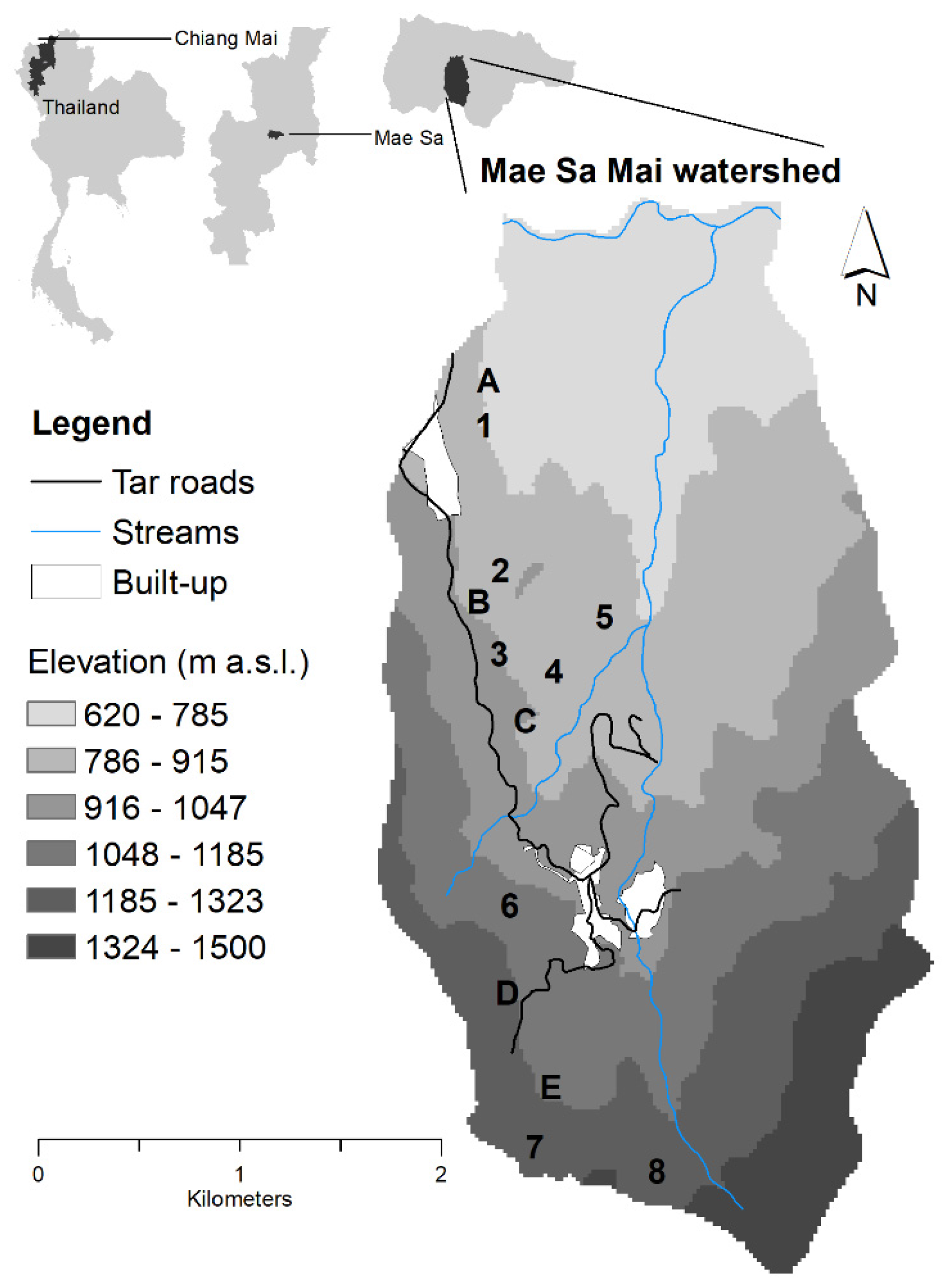
2.1. Study Area

The watershed of Mae Sa Mai was selected as the case study landscape because in tropical mountainous regions such as Northern Thailand, watersheds are critical spatial entities that provide important ecosystem services for society (e.g., carbon sinks, primary production, water cycling), and show distinct microclimate advantages (lower temperature, higher precipitation) for production of high-value crops such as vegetables. Mae Sa Mai watershed can be further regarded representative of areas in close proximities to regional market hubs (here: Chiang Mai city). The challenges the watershed faces have been also described for other mountainous regions of Mainland Southeast Asia [20] and tropical environments under transition, especially those with a strong dependence on agricultural production [11,19,21].
Mae Sa Mai watershed (MSMW) is a mountainous headwater catchment belonging to the larger Mae Sa basin. It is located at N 18°51′01′′ to E 98°52′20′′, about 40 km northwest of the provincial capital Chiang Mai City (Figure 1). MSMW covers an area of 10.6 km², and is sub-divided into Mae Sa Mai and Mae Sa Noi village, and the Queen Sirikit Botanical Garden. Topography is characterized by short, steep slopes, with small plateaus at elevation levels of 620 to 1440 m a.s.l. Soil types are predominantly Acrisols, Cambisols and to a smaller extent, Umbrisols [22]. A seasonal tropical climate prevails with a dry season from December to April and a rainy season from May to October, with an average annual precipitation of 1400 mm at 820 m a.s.l. [23].

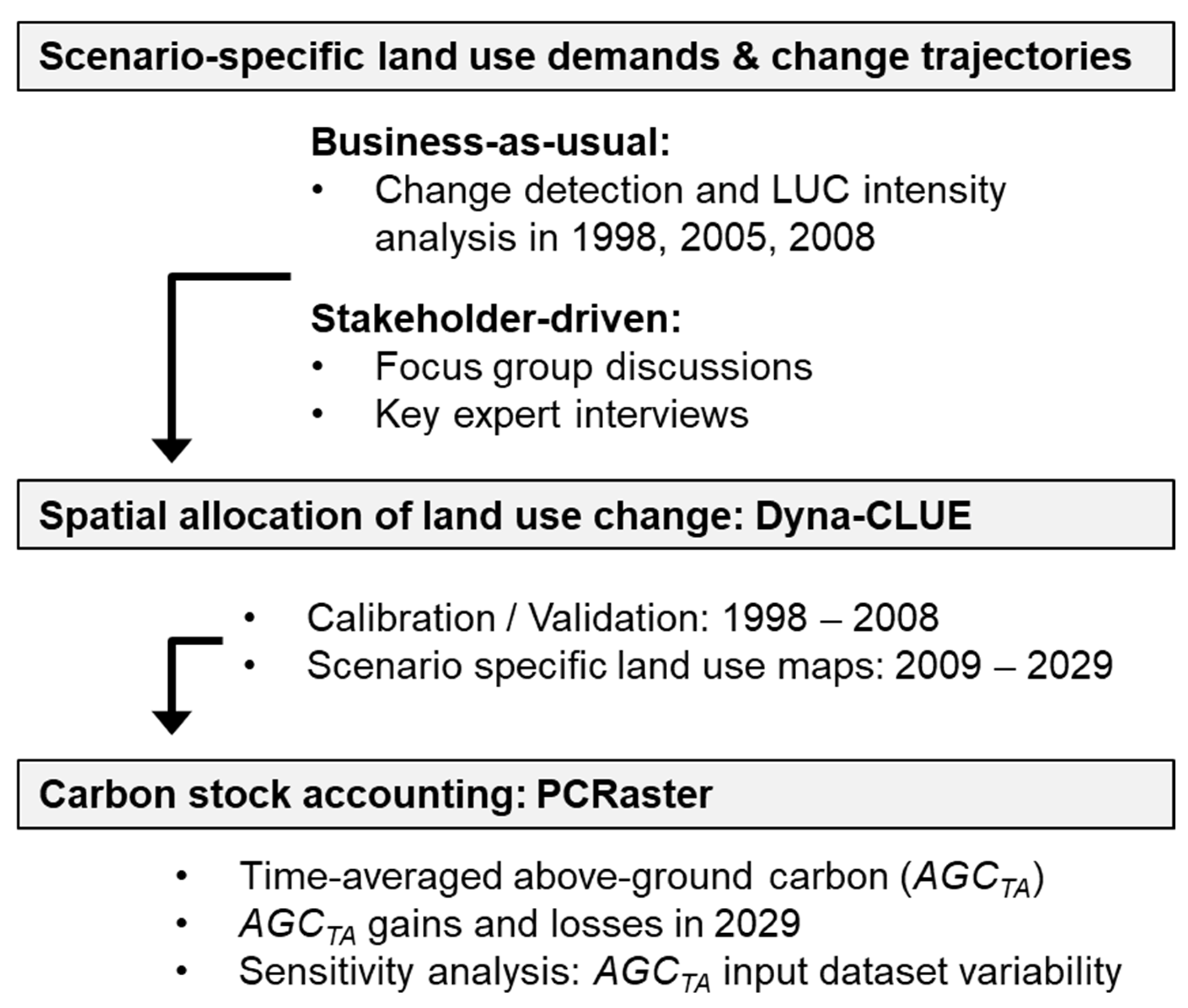
2.2. Scenario Development and Land-Use Change Modelling

An overview of the newly composed assessment framework is shown in Figure 2 with further descriptions presented in Section 2.2, Section 2.3 and Section 2.4.

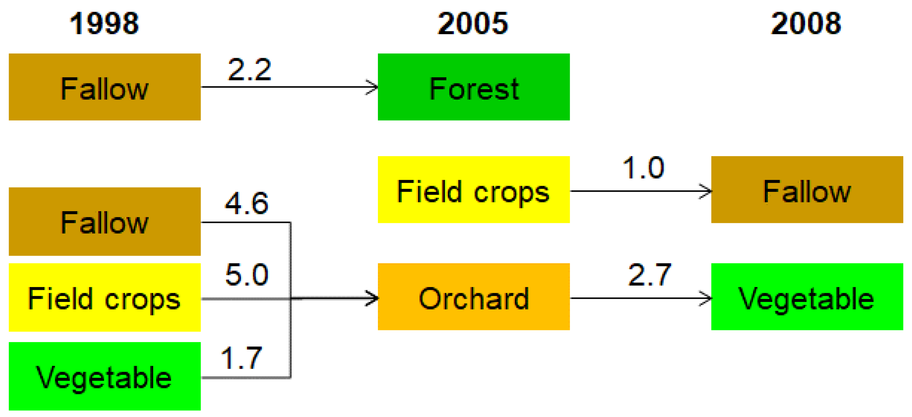
2.2.1. Land Use Change Analysis

An LUC analysis was conducted using available digitized and orthorectified secondary land-use maps referring to 1998 and 2005 [19,24], and our own field surveys in 2008. The originally reported twelve land-use classes in 1998 were merged into six land-use types (fallow, field crops, orchards, vegetables, secondary forests, built-up) to facilitate the analysis (Table 1). A wall-to-wall accuracy assessment that provides a statistical estimator of classified land use information (e.g., Kappa) [25] could not be conducted in this study because land-use maps for 1998 and 2005 were produced through a visual interpretation of printed aerial orthophotos in the field [19,24]. A similar approach was used for land-use patterns in 2008, building on a stratified field survey design, with land-use in 2005 as basic sampling unit as it resembled the local field owner structure and hence could be also regarded as a form of watershed land cadaster. For this purpose, MSMW was divided into eight sampling blocks; land-use patterns of 2005 were compared in the field with the observed patterns in November 2008 per sampling block. LUC was detected by visual comparison, for example, if cut-down fruit trees or newly established vegetable fields were detected in the field, the 2005 land-use map was updated accordingly. In addition, farmers of the identified LUC locations in 2008 were interviewed to crosscheck field observations and to serve as independent validation unit, respectively. Based on these approaches, an accuracy assessment as described above was not conducted because it was assumed that the interpretation of land-use types during field campaigns would lead to a realistic representation of land-use patterns during the observation years. The resulting land-use datasets were converted into raster format using a pixel size of 625 m² (25 × 25m) which corresponds to the smallest plot size of MSMW. All mapping work was done in ArcGIS 10.
Outcomes of the analysis were first used to detect the most recent land-use change patterns, and second, to identify gains and losses per land-use type trajectory during the assessment period of ten years.
The quantification of LUC between the observation years 1998, 2005 and 2008 was computed using a cross-tabular comparison to derive a transition matrix that identifies differences in extent of land-use type, and between two individual time periods. The second analysis step was described by [26] as ‘land-use intensity analysis’, which determines whether a land-use type i would have gained systematically from land-use type j and/or j lost systematically to i by:
Q t i j = ( C t i j / ( Y t + 1 Y t ) ) i j C t i j
where Qtij is the annual transition from land-use type i to j during time interval Yt+1 and Yt; Ctij is the number of pixels that transition from land-use type i at time interval Yt to land-use type j at time interval Yt+1; and t is the index of the initial time step of the interval (Yt, Yt+1). According to [26], the land-use intensity analysis does not require a minimum/maximum assessment period but needs at least three time periods for the analysis. It has to be further noted that the approach of [26] does not focus on analyzing crop yield intensification but focuses solely on spatial patterns of land-use intensification, expressed in percentage gains and losses, respectively.

2.2.2. Dyna-CLUE Modelling

The Dyna-CLUE model was chosen because its model complexity and spatial allocation algorithm, combined with its moderate data demands, has been proven valid in many tropical environments [12,27,28].

Calibration and Validation

Outcomes of the land-use change analysis were used as inputs to calibrate a Dyna-CLUE baseline scenario, using 1998 for calibration, and the reference years 2005 and 2008 for model validation. The calibrated model setting (for further details see also: Supplement S1) was evaluated for the period 1998–2008 (later referred to as ‘baseline scenario’), comparing the simulated land-use maps for 2005 and 2008 with their reference maps of the same years by using the goodness-of-fit (GOF) approach of [29]. The GOF approach compares the accuracy of the LUC model to the accuracy of its null model at multiple resolutions. A null model is defined as a model that assumes complete persistence of land-use across the simulated time period [29,30]. GOF requires three sets of maps to perform the analysis: (i) a reference map of the initial simulation year, e.g., land-use map 1998, (ii) a reference map of the final simulation year, e.g., land-use map 2008, and (iii) the corresponding land-use map as computed by Dyna-CLUE for 2008. The resulting GOF indicator (GOFt) compares the accuracy of the LUC model to the accuracy of its null model at multiple resolutions (ranging from 0 to 1, with 1 indicating a perfect model fit) [27].

Scenario-Specific Land-Use Demands and Simulated LUC Trajectories

Annual land-use demands for each scenario were set in the Dyna-CLUE model following a specific storyline and the spatial restrictions imposed by forest conservation areas and the Queen Sirikit botanical garden. Overall, five LUC scenarios were developed, with a summary of each scenario, and the methods and tools used to develop a specific storyline are presented in Table 2.
Scenario TREND extends the observed LUC patterns (2005–2008) up to 2029 based on the outcomes of the aforementioned land-use change analysis. A twenty-year scenario period was employed following the assumption of [10] that this period would be needed in the case of Thailand to halt deforestation nationwide. The OFF-FARM and CROP-SHIFT storylines build on participatory focus group discussions with 32 villagers, using adapted Participatory Appraisal techniques that were described in detail by [18]. In this case, participant groups were composed by a mixture of local key persons such as village headmen, farmers who cultivate plots in MSMW, and villagers not involved in any farming activities. Based on the participatory analysis, OFF-FARM scenario favors a 25% reduction in farming activities and related land-use demand compared to the observed LUC trends during 1998–2008. This reduction would be induced by increasing off-farm working opportunities and the abandonment of farming activities. Similar trends were also discussed by [31] to overcome the declining profitability of litchi orchards in Northern Thailand. By contrast, the CROP-SHIFT storyline simulates a continuous shift of vegetable fields to maize-based farming systems which was driven by local stakeholders’ expectation that regional livestock feed demands will increase in the near future.
According to [32], livestock feed demand started to increase in many countries of South-East Asia due to changes in consumer preferences towards dairy and meat products. The calibrated land- use change trajectories of CROP-SHIFT lead to an increased land competition between vegetable and field crop sites. In the case of CROP-SHIFT, orchard conversion rates were set 10% lower than the calibrated rates of TREND.
The REFOREST and NEW ORCHARD storylines were deduced from key expert interviews with officers of the District Department of Agriculture, the Department of Forestry, and the Royal Project Foundation, a non-governmental organization engaged in regional extension services. REFOREST follows the Department of Forestry’s vision to convert fallow and vegetable fields to reforestation sites in MSMW by an annual rate of two hectares. NEW ORCHARD follows an intervention scheme proposed by the Royal Project Foundation and the Department of Agriculture to introduce a new fruit tree species (Persimon spp.) as a means of farm product diversification. In the NEW ORCHARD storyline, the expansion of orchards is at the expense of field crop or vegetable fields. For this case, the expansion of the new orchard area was set to a similar rate of 2 ha per year to enable the comparison of above-ground carbon stock build-up rates with the REFOREST storyline.

2.3. Carbon-Stock Accounting Procedure

The impact of a specific LUC scenario on above-ground carbon per grid cell (625 m²) was assessed with the time-averaged carbon-stock accounting procedure of [16]. In the case of this study, soil carbon stocks were not considered because especially in tropical environments, maximum carbon sequestration can be often achieved by focusing more on aboveground carbon than on soil organic carbon due to smaller pool sizes and short mean residence times [7,8]:
Δ A G C T A ( t , t + 1 ) = A t [ i = 1 n ( a i , t ( A G C T A ( i , t + 1 ) A G C T A ( i , t ) ) + ( a i , t + 1 a i , t ) A G C T A ( i , t ) ) ]
where ΔAGCTA(t,t+1) is the annual change in time-averaged above-ground carbon stocks at the landscape scale (Mg ha−1); ai is the land-use-type-specific fraction of total area A (ha); AGCTA(i,t) is the land-use-type-specific time-averaged above-ground carbon stock density (Mg ha−1) and t is the time step (years). Time-averaged stock data have the advantage of allowing a comparison of land-use types with different rotation lengths and carbon sequestration potentials, especially important for agriculturally dominated land-use systems, such as fruit tree orchards or field crop systems [4,33,34].
Time-averaged above-ground carbon (AGCTA) budgets were computed with the environmental modelling language PCRaster [35] by soft-coupling the scenario-specific LUC maps of Dyna-CLUE with the carbon stock accounting procedure of [16]. The input data required to compute a land-use type-specific and time-averaged above-ground carbon stock were obtained from field measurements and literature. A summary of AGCTA input data is presented in Table 3. Further information of field data collection and the underlying assumptions to compute the AGCTA database are described in more detail in Supplement S2 and S3.

2.4. Sensitivity Analysis

A sensitivity analysis was performed to relate the variability of the carbon-stock accounting input factors to the uncertainty of the soft-coupled simulation results. The analysis basically relates the level of AGCTA per land-use type to the variability in the computed AGCTA stock level in 2029. Accordingly, coupled AGC-LUC simulations were executed separately in PCRaster using the reported average (AGCTA-AVG), minimum (AGCTA-MIN) and maximum (AGCTA-MAX) range of AGCTA inputs (Table 3), resulting in a total of 15 AGC-LUC coupling scenarios.

3. Results and Discussion

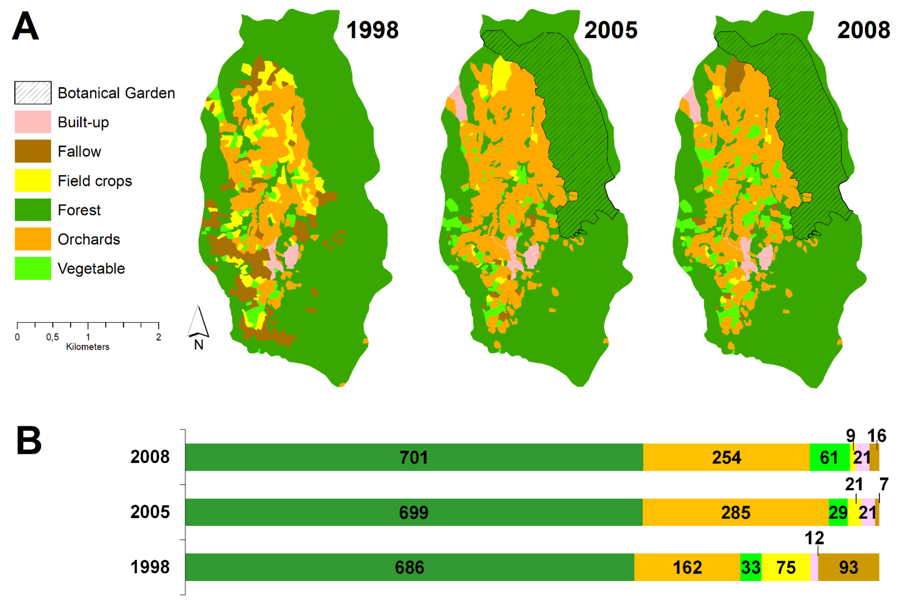
3.1. Spatial and Temporal Patterns of Land Use Change during 1998–2008

LUC patterns were mainly observed in the agricultural dominated areas of MSMW during the assessment period 1998–2008 (Figure 3A). For example, orchards increased from 162 ha in 1998 to 285 ha in 2005, and then fell again to 254 ha in 2008. By contrast, vegetable fields decreased from 33 ha in 1998 to 29 ha in 2005 and then rose to 62 ha in 2008. Field crops and fallow areas decreased continuously over the assessment period, with an area as low as 9 and 16 ha, respectively, in 2008. Built-up areas including residential houses, buildings related to the botanical garden, and paved surfaces increased to 20 ha in 2005 and remained stable thereafter. Secondary forests were the dominant land-use form in MSMW, covering approximately 70% or 700 ha of the total watershed area in 2008 (Figure 3B).
The land use-change intensity analysis (Equation (1)) detected four dominating LUC trajectories during 1998–2008 (Figure 4). In the period 1998–2005, one LUC trajectory referred to the increase of orchard plantations at the expense of fallow (−4.6%), field crops (−5.0%) and vegetable fields (−1.7%). A second trajectory could be related to the conversion of fallow (−2.2%) into secondary forest areas. Both trajectories came to a halt in 2006–2008, where two new trajectories were detected with one leading to the conversion of field crop areas into fallow land (+1.0%), and a second one that led to the conversion of orchards into vegetable fields (+2.7%).
Identified land-use change trajectories for the case of Mae Sa Mai watershed were also described by [43,44,45] in particular for the case of Mainland Southeast Asia. Land use intensifications mainly occurred as a series of push and pull factors that were often characterized by a mixture of economic and policy incentives. For example, the overall decrease in field crop and fallow field during 1998–2005 was driven by a push induced by a government initiative to reduce swiddening management practices in Northern Thailand [44,45]. During the same period, emerging cash crop opportunities and market-driven incentives led to the pull that drove the expansion of orchard areas [12]. The period 2006–2008 was characterized by a drop of litchi farm-gate prices that led to an increase of vegetable production areas spurred by increasing regional consumer demands for fresh vegetables [46]. Another pull was attributed to the increase in secondary forest areas due to national reforestation initiatives [11]. However, this pull was not directly detectable in the land-use change intensity analysis, as reforestation and secondary forests were merged into a single land-use class. An additional land-use type ‘reforestation’ would have been more suitable in this case. But as landscape features in tropical environments often appear in continuous gradients from small-scale subsistence to more homogenous landscape features, it is often difficult to simplify and classify landscapes by distinguishing discrete features one from another [47]. This was also seen in the relatively steep increase of built-up areas observed during 1998–2005, as the increase was mainly attributed to the construction of a new royal project foundation field station, and not necessarily attributed to the expansion of settlement areas.

3.2. Dyna-CLUE Modelling

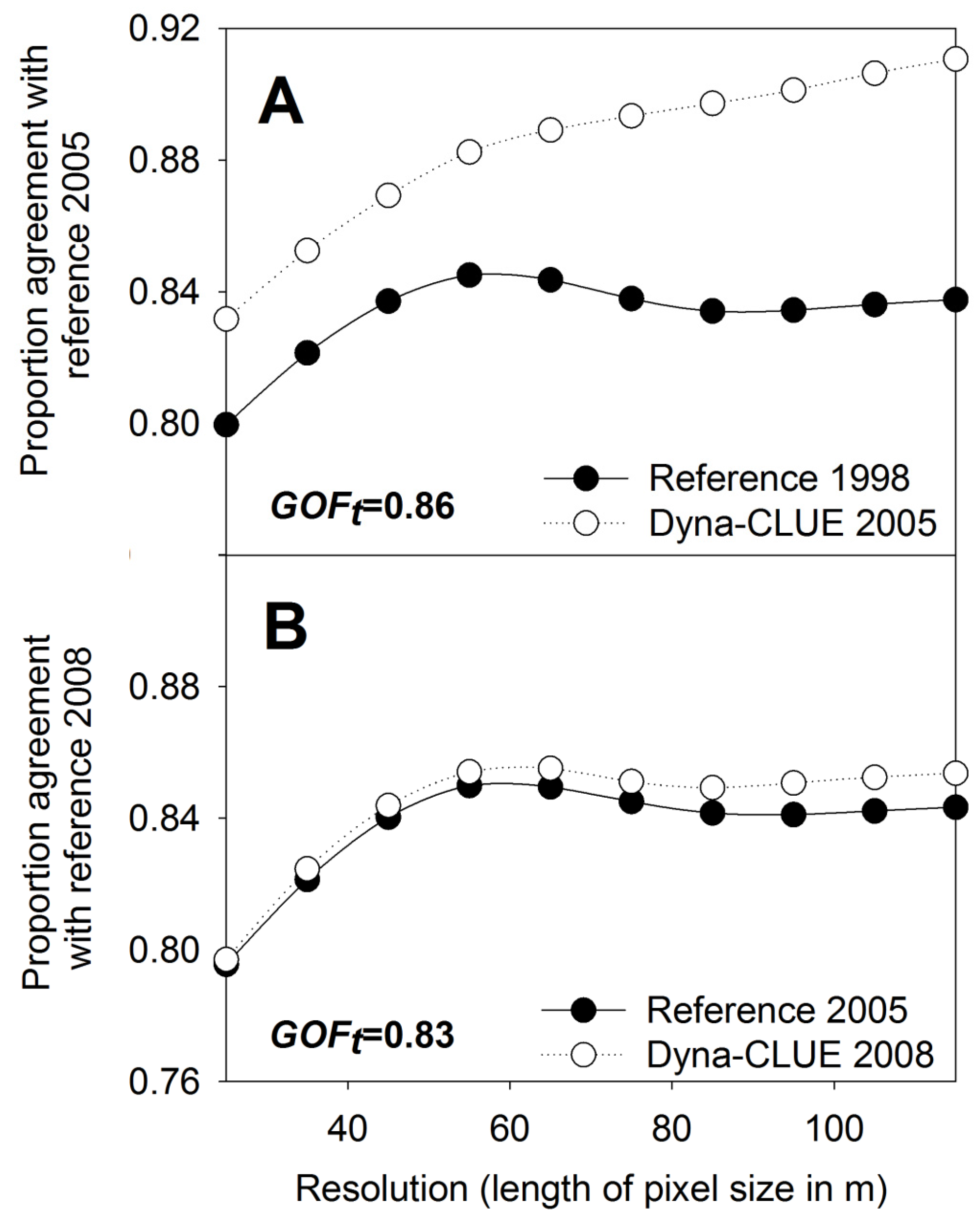
3.2.1. Significance of Baseline Regression Coefficients and Model Validation

The logit models that generated the regression coefficients for the baseline scenario calibration were able to explain the spatial occurrence of land-use types in MSMW in acceptable ranges as demonstrated by the satisfactory to good ROC values 0.74 (vegetable) and 0.98 (urban). Not all factors that were used in the regression computations were significant at p < 0.05 and those that were significant differed as a function of land-use type and prediction variable (Table S1).
For example, the location factor ‘distance-to-road’ was significant for orchards, which can be explained by the need to access plantations by pickup trucks. The factors ‘distance-to-streams’ and ‘road networks’ were significant for vegetables which can be explained by the need for irrigation water during dry seasons and motorized transportation of fresh products to nearby market hubs. Although expected, there was no significant correlation between soil type and occurrence of field crops or vegetable fields. This was probably related to the high fertilizer rates applied in MSMW, which do not necessarily result in fertile soil types.
The baseline model validation which refers to the simulated land-use maps of TREND scenario in 2005 and 2008 was compared with their corresponding land-use maps. The result revealed that simulations were more accurate than the null model at all resolutions (25 to 125 m). This was further confirmed by goodness-of-fit (GOFt) coefficients that were in the range of 0.80 to 0.91 (Figure 5) in both assessments periods.
The GOFt computations revealed that the agreement between simulated and observed land-use patterns during the examined baseline scenario period (1998–2008) was rather high (0.83–0.86) compared to other regional studies that relied on the Dyna-CLUE as LUC modelling engine [18,28,48]. One reason could be the relative large secondary forest cover (approximately 70%) in MSMW that did not substantially change in size or location during the assessment period from 1998–2008. But as the spatial validation procedure of [29] determines the fit between two maps across multiple resolutions, it becomes evident that the area of secondary forests was therefore predicted well at the initial resolution of 25 m. Nevertheless, the chosen validation procedure refers to standard LUC model validation approaches, and further follows the plea of [49] to validate modelling results with historic land-use data.

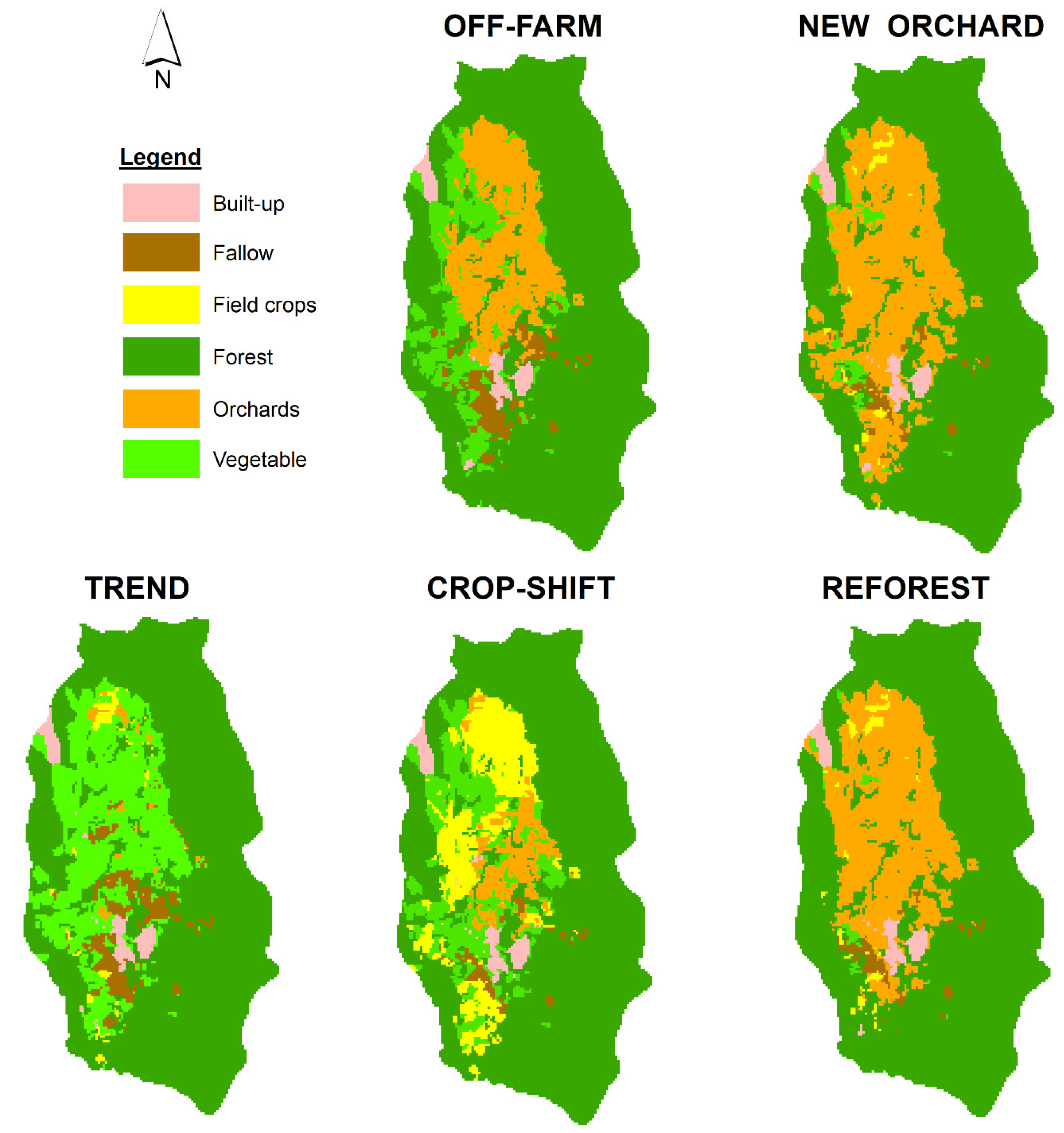
3.2.2. Scenario Analysis

The TREND scenario computations resulted in an almost complete conversion of orchards into vegetable fields by 2029 and the further clustering of fallow areas in close proximity to village areas (Figure 6). The stakeholder-driven LUC trends simulated with the OFF-FARM storyline projected vegetable fields close to roads, orchards remaining in the central valley bottom, and fallow fields occurring in close distance to the villages. The CROP-SHIFT storyline resulted in the formation of a field crop cluster in the northern, western or southern part of MSMW, and an orchard cluster in the central valley bottom. The spatial patterns simulated by NEW ORCHARD showed similar visual patterns as OFF-FARM computations, but differed by a projected larger vegetable area in the western part of MSMW. The LUC trajectories simulated by the REFOREST storyline led to an increase of secondary forest sites on the expense of agriculturally dominated land-use types. This was especially prominent in the southern part of MSMW, where the majority of new secondary forests plots were projected at high elevation and steep sloping locations.
The simulated scenario storylines suggested that future LUC patterns in MSMW will be mainly driven by external factors such as markets demands and environmental policies. Simulations further revealed that agriculture and cash crop production systems will remain important land-use components in 2029, but characterized by two slightly different LUC trajectory directions. Firstly, stakeholder-driven LUC patterns will lead to a continuation of land-use intensification that is driven by cash crop production, as also simulated with the CROP-SHIFT storyline. A similar trend was also described by [50], who could show that a continuous expansion of mono-cultural maize cropping leads to soil fertility decline and land degradation in the long run. The trend to expand vegetable production could be attributed to the promise of higher economic returns compared to declining litchi farm gate prices that started in 2006. Given the ongoing changes in consumer preferences [46], this trend will substantially influence upland farming patterns in Northern Thailand over the next decades [11].
The scenario analysis further revealed that an increase in off-farm working opportunities may further serve as an endogenous LUC driver, leading in this case to a reduction in land-use intensification patterns as simulated by the OFF-FARM storyline. Schreinemachers et al. [31] also observed that seasonal and even permanent migration of rural labor has started to influence the labor-intensive farm management practices in Northern Thailand, especially for areas in close proximity to urban centers such as Chiang Mai. Compared to market-demand-driven LUC scenarios described above, the institutionally-driven scenario storylines NEW ORCHARD and REFOREST focused on long-term land-use strategies favoring the built-up of above-ground carbon stocks. Although relevant from a carbon sequestration point of view, these storylines counteract stakeholder demands for fast economic returns as shown by CROP-SHIFT. This is because fruit trees are not productive in the first years of cultivation, and current reforestation policies in Thailand do not foresee economic returns unless financial remuneration or compensation payments will be achieved, for example, through a REDD+ project. But it is still questionable whether a fruit-tree-based land-use system can be economically viable due to rising labor costs [31]. Hence, it is important to provide other economic incentives for local orchard farmers, for example, through product certification or post-harvest product enhancements, to ensure the viability of fruit-tree-based farming systems in MSMW in the long run [11].

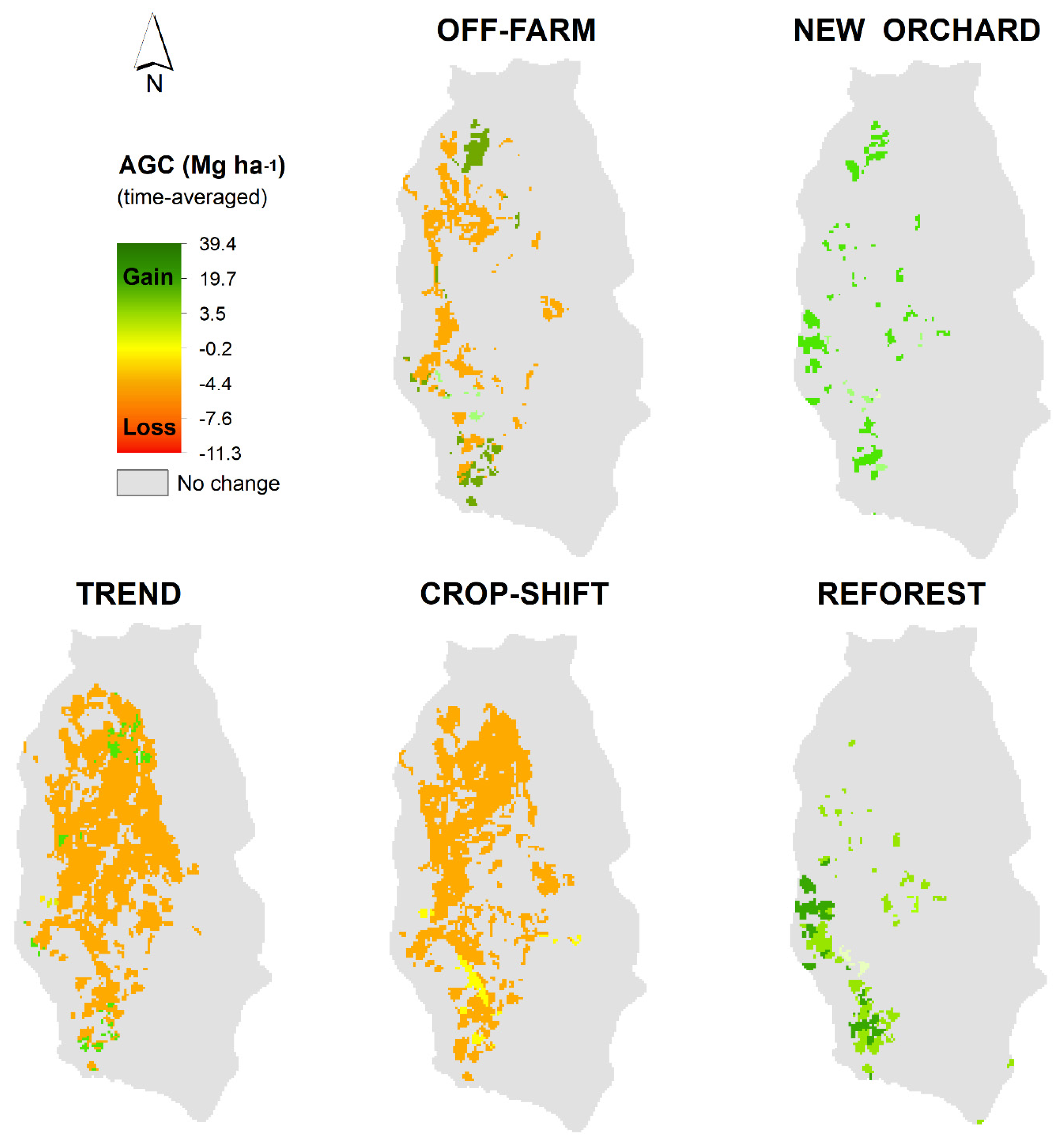
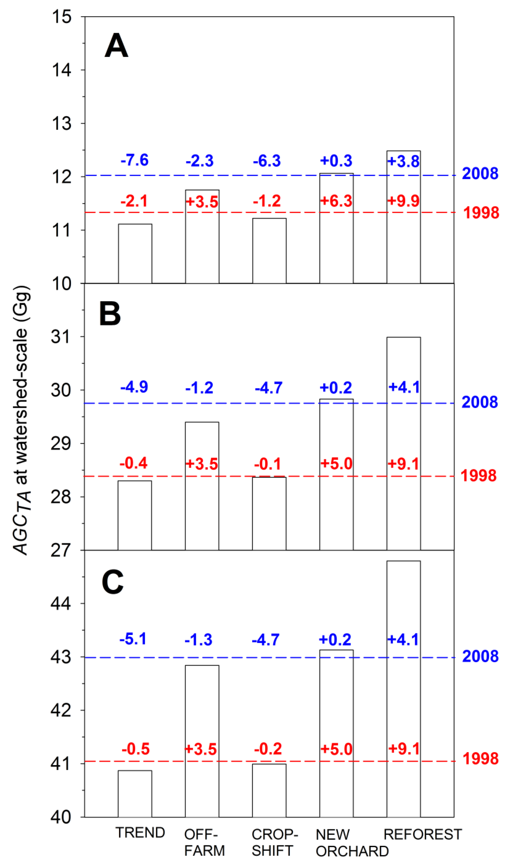
3.3. Impacts of Land-Use Change on Above-Ground Carbon Stocks and Implications for Environmental Management

The coupled LUC-AGC computations resulted in time-averaged AGC stock gains of 12 to 43 Gg, depending on employed input dataset, at the level of MSMW by 2029 (Figure 7). As a function of calibrated AGCTA input dataset, up to 1.7 Gg additional AGC could be achieved due to increasing reforestation and orchard areas.
On the contrary, up 0.4 Gg AGC stocks would be lost if current LUC trends continue until 2029. Unsurprisingly, LUC transitions that resulted in a conversion of perennial (fallow, orchards) to annual cropping systems depicted the largest reductions in time-averaged above-ground carbon stocks. Especially for those scenarios that favored a conversion of orchards into vegetable or field crop systems (TREND, OFF-FARM and CROP-SHIFT), above-ground carbon decreased by 1.2% (OFF-FARM) to 7.6% (TREND) at the watershed-scale.
This corresponds to a decrease of 0.45 to 1.01 Gg of above-ground carbon compared to the base year 2008 (Figure 8). TREND and CROP-SHIFT scenarios resulted in the overall largest above-ground carbon losses, independent of employed AGCTA input data level, off-setting the above-ground carbon gains achieved during 1998 to 2008. In contrast, LUC scenarios which favored a reduction in vegetable or field crop areas (NEW ORCHARD, REFOREST) lead to increase of above-ground carbon by 0.2 to 4.1% or 0.1 to 1.7 Gg until 2029. Coupled simulations also demonstrated distinctively different spatial patterns of above-ground carbon sources and sinks at the watershed scale by 2029. For example, the LUC pattern simulated in TREND leads to above-ground carbon losses of up to 7.7 Mg ha−1 for those grid cells where orchards were replaced by vegetable fields (Figure 7). By contrast, an increase in fallow or reforestation areas fostered the build-up of new above-ground carbon stocks, as is to be expected. This was, for example, prominent in the REFOREST scenario with new above-ground carbon stocks being computed in the range of 29–39 Mg AGCTA ha−1 on steep slopes and ridge-top locations. Different patterns were seen in the OFF-FARM simulations, where new above-ground carbon stocks were simulated to occur in the northern and south-western parts of MSMW instead.
The establishment of new tree plantations or reforestation areas is promoted by government agencies [10] as one of the most promising methods of building up long-term above-ground carbon stocks, as demonstrated by NEW ORCHARD or REFOREST scenarios. Nevertheless, there can be large variations in carbon sequestration potentials depending on tree species planted, management practices and local environmental conditions [4]. The reported minimum and average above-ground carbon stock data that were used in the carbon-stock accounting procedure were comparable to other studies in South-East Asia [3,4]. However, the maximum time-averaged above-ground carbon stock data computed with the coupled modelling procedure in 2029 were in parts higher than other estimates for tropical environments [51,52] as a result of overall wide range of values reported in literature. This type of uncertainty could be captured fairly well by the sensitivity analysis, further revealing the wide variation in prospected above-ground carbon stocks for 2029. This also highlights the importance of building on local above-ground carbon datasets instead of relying on default information from national or carbon stock assessment guidelines [6]. Ground-based inventories are essential because most satellite or aerial monitoring techniques, which many national carbon-emission-reporting strategies rely on, still exhibit limitations in adequately distinguishing between different tree-based land-use systems such as agroforests or small-scale landscape mosaics [4]. Furthermore, there is still a great uncertainty in many tropical landscapes regarding how much soil organic carbon (SOC) exists due to a lack of reference information, particularly for deep soils high in organic material [4]. Greatest losses of soil organic carbon are expected to occur shortly after forest conversion, but further long-lasting reductions in SOC may continue due to land use intensification, e.g., abandonment of fallow periods or mono-cultural cropping systems.

3.4. Local Stakeholders as Key Partners of Environmental Management

The range in scenario-specific above-ground carbon stock gains and losses highlights the trade-offs of agricultural production and economic incentives compared to long-term carbon sequestration goals. This contradicts current national policy concepts that attempt to integrate both concepts into a single framework [53]. It is further questionable whether focusing on a single land-use management goal such as long-term AGC sinks will be beneficial in the long-run. In the case of Thailand, current land-use policies counteract local stakeholder needs, as local LUC trajectories may not follow regional or national LUC trends upon which many policy decisions rely [36,43]. This conflict of objectives is the result of contrasting land-use policies that further challenge the implementation of policy frameworks such as REDD+. It is more important to acknowledge the local socio-ecological diversity and to rely on a mixture of socio-economical and ecosystem incentives that support the co-design of carbon sequestration needs and agricultural development pathways. By this means, spatial goal conflicts that were depicted through the scenario analysis, e.g., reforestation vs. agriculture, could be avoided. Neef [11] argued that incentive-based policies that are achieved through multi-stakeholder partnerships are necessary to overcome the current antagonisms of conservation and development strategies in landscapes such as MSMW.
Additionally, consideration must be also given to the format in which such findings are communicated to local stakeholders. For example, LUC and above ground carbon-stock maps generated by this study offer a visual interpretation of future LUC trajectories that statistical reports are unable to convey to local stakeholders or policymakers. Although there is little doubt that maps are powerful visualization tools, there is also the danger that a modelled scenario may be seized upon as a definite result. Hence, it is crucial to ensure that the ‘map end-users’ are aware of the embedded methodological limitations and uncertainties, e.g., as described for the land-use maps 1998–2008, through transparent communication strategies, putting researchers into the role of active mediators rather than mere observers. This emphasizes the usefulness of the participatory-driven storylines that demonstrated the land-use conflict potential in the context of MSMW, and many other watersheds in Southeast Asia or tropical environments. Taking local stakeholders’ viewpoints and assumptions into consideration is especially relevant for the development of integrated environmental management strategies at landscape level. This is paramount because it increases the credibility of environmental policies for local communities, but require stakeholders to be acknowledged as key partners in the development of sustainable environmental management approaches, rather than being perceived merely as adopters of top-down national environmental policies.

4. Conclusions

Efforts to reduce the impact of LUC on above-ground carbon pools and to establish sustainable climate mitigation mechanisms are currently being challenged by the intensification of agricultural production in many tropical landscapes. The combination of participatory approaches and modelling tools is particularly useful in data-limited environments such as Northern Thailand for the simulation of scenarios based on local stakeholder assumptions. The modelling tools that were part of the newly composed assessment approach build on Dyna-CLUE and PCRaster that were used to couple the carbon stock accounting procedure with the simulated LUC trajectories. The combination of these tools was beneficial not only on account of their moderate data requirements, but also because they enabled the comparison of land-use systems with different above-ground carbon build-up rates and rotation times. The use of LUC scenarios based on local stakeholder assumptions offers higher credibility for climate mitigation and environmental management strategies at the landscape level, further underlining the need to co-design policy frameworks that acknowledge local stakeholder needs.

Supplementary Materials

The following are available online at www.mdpi.com/2073-445X/6/4/85/s1.

Acknowledgments

The authors would like to thank the villagers of Mae Sa Mai and Mae Sa Noi and the members of the Upland office, Chiang Mai, Thailand, for their support during the course of study. This research was conducted within the framework of the Collaborative Research Programme “Sustainable Land use and Rural Development in Mountainous Regions of Southeast Asia” (SFB 564, The Uplands Program). The financial support of the Deutsche Forschungsgemeinschaft DFG (German Research Foundation) is gratefully acknowledged.

Author Contributions

M.L. and T.H. conceived and designed the research; M.L. conducted the analysis; M.L., S.S. and N.W. performed the field experiments; M.L. analyzed the data; M.L., T.H., A.J. and G.C. wrote the paper.

Conflicts of Interest

The authors declare no conflict of interest. The funding sponsors had no role in the design of the study; in the collection, analyses, or interpretation of data; in the writing of the manuscript, and in the decision to publish the results.

References

  1. Houghton, R.A.; House, J.I.; Pongratz, P.; van der Werf, G.R.; DeFries, R.S.; Hansen, M.C.; Le Quéré, C.; Ramankutty, N. Carbon emissions from land use and land-cover change. Biogeoscienes 2012, 9, 5125–5142. [Google Scholar] [CrossRef]
  2. Jansen, L.J.M.; Di Gregorio, A. Parametric land-cover and land-use classifications as tools for environmental change detection. Agric. Ecosyst. Environ. 2002, 91, 89–100. [Google Scholar] [CrossRef]
  3. Bruun, T.B.; de Neergaard, A.; Libach Burup, M.; Hepp, C.M.; Nylandsted Larsen, M.; Abel, C.; Aumtong, S.; Magid, J.; Mertz, O. Intensification of Upland Agriculture in Thailand: Development or Degradation? Land Degrad. Dev. 2016, 28, 83–94. [Google Scholar] [CrossRef]
  4. Ziegler, A.; Phelps, J.; Qi Yuen, J.; Webb, E.L.; Lawrence, D.; Fox, J.M.; Bruun, T.B.; Leisz, S.J.; Ryan, C.M.; Dressler, W.; et al. Carbon outcomes of major land-cover transitions in SE Asia: Great uncertainties and REDD+ policy implications. Glob. Chang. Biol. 2012, 18, 3087–3099. [Google Scholar] [CrossRef] [PubMed]
  5. Foley, J.A.; DeFries, R.; Asner, G.P.; Barford, C.; Bonan, G.; Carpenter, S.; Chapin, F.S.; Coe, M.T.; Daily, G.C.; Gibbs, H.K.; et al. Global consequences of land use. Sci. Total Environ. 2005, 309, 570–574. [Google Scholar] [CrossRef] [PubMed]
  6. UNFCCC. United Nations Framework Convention on Climate Change Outcome of the Ad Hoc Working Group on Long-term Cooperative Action under the Convention. Available online: http://unfccc.int/meetings/durban_nov_2011/meeting/6245.php (accessed on 5 April 2012).
  7. Bruun, T.B.; de Neergard, A.; Lawrence, D.; Ziegler, A.D. Environmental Consequences of the Demise in Swidden Cultivation in Southeast Asia: Carbon Storage and Soil Quality. Human Ecol. 2009, 37, 375–388. [Google Scholar] [CrossRef]
  8. Lal, R. Soil carbon sequestration to mitigate climate change. Geoderma 2004, 123, 1–22. [Google Scholar] [CrossRef]
  9. Fox, J.; Vogler, J.B.; Sen, O.L.; Giambelluca, T.W.; Ziegler, A.D. Simulating land-cover change in montane mainland Southeast Asia. Environ. Manag. 2012, 49, 968–979. [Google Scholar] [CrossRef] [PubMed]
  10. ONEP-Office of Natural Resources and Environmental Policy and Planning. Thailand’s Second National Communication under the United Nations Framework Convention on Climate Change; Ministry of Natural Resources and Environment: Bangkok, Thailand, 2010; p. 102.
  11. Neef, A. Fostering incentive-based policies and partnerships for integrated watershed Management in the Southeast Asian uplands. Southeast Asian Stud. 2012, 1, 247–271. [Google Scholar]
  12. Trébuil, G.; Ekasingh, B.; Ekasingh, M. Agricultural commercialisation, diversification, and conservation of renewable resources in northern Thailand highlands. Moussons. Recherche en Sciences Humaines sur l’Asie du Sud-Est 2006, 9–10, 131–155. [Google Scholar]
  13. Plieninger, T. Monitoring directions and rates of change in trees outside forests though multitemporal analysis of map sequences. Appl. Geogr. 2012, 32, 566–576. [Google Scholar] [CrossRef]
  14. Sumarga, E.; Hein, L. Mapping ecosystem services for land use planning, the case of Central Kalimantan. Environ. Manag. 2014, 54, 84–97. [Google Scholar] [CrossRef] [PubMed]
  15. Lusiana, B.; van Noordwijk, M.; Cadisch, G. Land sparing or sharing? Exploring livestock fodder options in combination with land use zoning and consequences for livelihoods and net carbon stocks using the FALLOW model. Agric. Ecosyst. Environ. 2012, 159, 145–160. [Google Scholar] [CrossRef]
  16. Van Noordwijk, M.; Suyamto, D.A.; Lusiana, B.; Ekadinata, A.; Hairiah, K. Facilitating agroforestation of landscapes for sustainable benefits: Tradeoffs between carbon stocks and local development benefits in Indonesia according to the FALLOW model. Agric. Ecosyst. Environ. 2008, 126, 98–112. [Google Scholar] [CrossRef]
  17. Anselme, B.; Bousquet, B.; Lyetc, A.; Etienne, M.; Fady, B.; LePage, C. Modelling of spatial dynamics and biodiversity conservation on Lure mountain (France). Environ. Model. Softw. 2010, 25, 1385–1398. [Google Scholar] [CrossRef]
  18. Lippe, M.; Thai Minh, T.; Neef, A.; Hilger, T.; Hoffmann, V.; Lam, N.T.; Cadisch, G. Building on qualitative datasets and participatory processes to simulate land use change in a mountain watershed of Northwest Vietnam. Environ. Model. Softw. 2011, 26, 1454–1466. [Google Scholar] [CrossRef]
  19. Verburg, P.H.; Overmars, K.P.; Huigen, M.G.A.; de Groot, W.T.; Veldkamp, A. Analysis of the effects of land use change on protected areas in the Philippines. Appl. Geogr. 2006, 26, 153–173. [Google Scholar] [CrossRef]
  20. Valentin, C.; Agus, F.; Alamban, R.; Boosaner, A.; Bricquet, J.P.; Chaplot, V.; de Guzman, T.; de Rouw, A.; Janeau, J.L.; Orange, D.; et al. Runoff and sediment losses from 27 upland catchments in Southeast Asia: Impact of rapid land use changes and conservation practices. Agric. Ecosyst. Environ. 2008, 124, 225–238. [Google Scholar] [CrossRef]
  21. Flotemersch, J.E.; Leibowitz, S.G.; Hill, R.A.; Stoddard, J.L.; Thoms, M.C.; Tharme, R.E. A watershed integrity definition and assessment approach to support strategic management of watersheds. River Res. Appl. 2016, 32, 1654–1671. [Google Scholar] [CrossRef]
  22. Schuler, U.; Herrmann, L.; Ingwersen, J.; Erbe, P.; Stahr, K. Comparing mapping approaches at subcatchment scale in northern Thailand with emphasis on the Maximum Likelihood approach. Catena 2010, 81, 137–171. [Google Scholar] [CrossRef]
  23. Fröhlich, H.; Schreinemachers, P.; Stahr, K.; Clemens, G. Policies and Innovations for Sustainable Land Use and Rural Development in Mountain Areas of Southeast Asia; Springer: Heidelberg, Germany, 2013; p. 490. [Google Scholar]
  24. Wünscher, T. Land Use Map of Mae Sa Mai Watershed 09/1998, Scale 1:10.000, Institute 490; University of Hohenheim: Stuttgart, Germany, 1998. [Google Scholar]
  25. Lillesand, T.M.; Kiefer, R.W. Remote Sensing and Image Interpretation, 4th ed.; Wiley & Sons: New York, NY, USA, 2000; p. 724. [Google Scholar]
  26. Aldwaik, S.Z.; Pontius, R.G. Intensity analysis to unify measurements of size and stationarity of land changes by interval, category, and transition. Landsc. Urban Plan. 2012, 106, 103–114. [Google Scholar] [CrossRef]
  27. Castella, J.-C.; Verburg, P.H. Combination of process-oriented and pattern-oriented models of land use change in a mountain area of Vietnam. Ecol. Model. 2007, 202, 410–420. [Google Scholar] [CrossRef]
  28. Trisurat, Y.; Alkemade, R.; Verburg, P.H. Projecting Land-Use Change and Its Consequences for Biodiversity in Northern Thailand. Environ. Manag. 2010, 45, 626–639. [Google Scholar] [CrossRef] [PubMed]
  29. Costanza, R. Model goodness of fit: A multiple resolution procedure. Ecol. Model. 1989, 47, 199–215. [Google Scholar] [CrossRef]
  30. Pontius, R.G.; Boersma, W.; Castella, J.-C.; Clarke, K.; de Nijs, T.; Dietzel, C.; Duan, Z.; Fotsing, E.; Goldstein, N.; Kok, K.; et al. Comparing the input, output, and validation maps for several models of land change. Annu. Reg. Sci. 2008, 42, 11–37. [Google Scholar] [CrossRef]
  31. Schreinemachers, P.; Potchanasin, C.; Berger, T.; Royrong, S. Agent-based assessment modeling for ex-ante assessment of tree crop innovations: Litchis in northern Thailand. Agric. Econ. 2010, 41, 519–536. [Google Scholar] [CrossRef]
  32. FAO. World Livestock 2011—Livestock in Food Security; FAO: Rome, Italy, 2011; p. 130. [Google Scholar]
  33. Hariah, K.; Dewi, S.; Agus, F.; Velarde, S.; Ekadinata, A.; Rahayu, S.; van Noordwijk, M. Measuring Carbon Stocks Across Land Use Systems: A Manual. Bogor, Indonesia; World Agroforestry Centre (ICRAF), SEA Regional Office: Nairobi, Kenya, 2011; p. 154. [Google Scholar]
  34. Yang, X.; Blagodatsky, S.; Lippe, M.; Liu, F.; Hammon, J.; Xu, J.; Cadisch, G. Land-use change impact on time-averaged carbon balances: Rubber expansion and reforestation in a biosphere reserve, South-West China. For. Ecol. Manag. 2016, 372, 149–163. [Google Scholar] [CrossRef]
  35. PCRaster. Available online: http://www.pcraster.geo.uu.nl (accessed on 18 August 2012).
  36. Thomas, D.; Preechapanya, P.; Saipothong, P. Landscape Agroforestry in Upper Tributary Watersheds of Northern Thailand. J. Agric. 2002, 18, 1–36. [Google Scholar]
  37. Matsumoto, N.; Paisancharoen, K.; Hakamata, T. Carbon balance in maize fields under cattle manure application and no-tillage cultivation in Northeast Thailand. Soil Sci. Tillage 2008, 54, 277–288. [Google Scholar] [CrossRef]
  38. Fukushima, M.; Kanzaki, M.; Hara, M.; Ohkubo, T.; Preechapanya, P.; Choocharon, C. Secondary forest succession after the cessation of swidden cultivation in the montane forest area in Northern Thailand. For. Ecol. Manag. 2008, 225, 1994–2006. [Google Scholar] [CrossRef]
  39. Kaewkron, P.; Kaewkla, N.; Thummikkapong, S.; Punsang, S. Evaluation of carbon storage in soil and plant biomass of primary and secondary mixed deciduous forests in the lower northern part of Thailand. Afr. J. Environ. Sci. Technol. 2011, 5, 8–14. [Google Scholar]
  40. Terakunpisut, J.; Gajaseni, N.; Ruankawe, N. Carbon sequestration potential in above-ground biomass of Thong Pha Phum National Forest, Thailand. Appl. Ecol. Environ. Res. 2007, 5, 93–102. [Google Scholar] [CrossRef]
  41. Petsri, S.; Pumijumnong, N. Above-ground carbon content in mixed deciduous forest and teak plantations. Environ. Nat. Resour. 2007, 5, 1–10. [Google Scholar]
  42. Gnanavelrajah, N.; Shresta, R.P.; Schmidt-Vogt, D.; Samarakoon, L. Carbon stock assessment and soil carbon management in agricultural land-uses in Thailand. Land Degrad. Dev. 2008, 19, 242–256. [Google Scholar] [CrossRef]
  43. Fox, J.; Vogler, J.B. Land-Use and Land-Cover Change in Montane Mainland Southeast Asia. Environ. Manag. 2005, 36, 394–403. [Google Scholar] [CrossRef] [PubMed]
  44. Hares, M. Forest conflict in Thailand: Northern minorities in focus. Environ. Manag. 2009, 43, 381–395. [Google Scholar] [CrossRef] [PubMed]
  45. Vanwambeke, S.O.; Somboon, P.; Lambin, E.F. Rural transformation and land use change in northern Thailand. Land Use Sci. 2008, 2, 1–29. [Google Scholar] [CrossRef]
  46. Lippe, R.S.; Seebens, H.; Isvilanonda, S. Urban Household Demand for Fresh Fruits and Vegetables in Thailand. Appl. Econ. J. 2010, 17, 1–26. [Google Scholar]
  47. Ardli, E.R.; Wolff, M. Land use and land cover change affecting habitat distribution in the Segara Anakan lagoon, Java, Indonesia. Reg. Environ. Chang. 2008, 9, 235–243. [Google Scholar] [CrossRef]
  48. Lusiana, B.; Suyamto, D.A.; van Noordwijk, M.; Mulia, R.; Joshi, L.; Cadisch, G. User’s perspective on validity of a simulation model for natural resource management. Int. J. Agric. Sustain. 2011, 9, 364–378. [Google Scholar]
  49. Verburg, P.H. Simulating feedbacks in land use and land cover change models. Landsc. Ecol. 2006, 21, 1171–1183. [Google Scholar] [CrossRef]
  50. Yap, V.Y.; de Neergaard, A.; Bruun, T.B. “To adopt or not to adopt?Legume adoption in maize-based systems of Northern Thailand: Constraints and potential. Land Degrad. Dev. 2017, 28, 731–741. [Google Scholar] [CrossRef]
  51. Becknell, J.M.; Kissing Kucek, L.; Powers, J.S. Aboveground biomass in mature and secondary seasonally dry tropical forests: A literature review and global synthesis. For. Ecol. Manag. 2012, 276, 88–95. [Google Scholar] [CrossRef]
  52. Palm, C.A.; Woomer, P.L.; Alegree, J.; Arevaldo, L.; Castilla, C.; Cordeiro, D.G.; Feigl, B.; Hariah, K.; Kotto-Same, J.; Mendes, A.; et al. Carbon Sequestration and Trace Gas Emissions in Slash-and-Burn and Alternative Land-Uses in the Humid Tropics; Final Report, Phase II, (TSBF); ASB Climate Change Working Group: Nairobi, Kenya, 2000. [Google Scholar]
  53. Laosuwan, T.; Utturak, P. Review of methods and potential role of remote sensing forest carbon stock measurement: A pilot project for REDD+ in Thailand. Int. J. Geoinform. 2013, 9, 39–48. [Google Scholar]
Figure 1. Location of Mae Sai Mai watershed (MSMW) in Chiang Mai province, Northern Thailand, indicating topographic and infrastructure features, and locations of above-ground biomass field measurements, with 1 to 8 referring to litchi orchards, A to E cabbage plots (for explanation see also: Supplemental Material S2 and S3).
Land 06 00085 g001
Figure 2. Conceptual study framework.
Land 06 00085 g002
Figure 3. Spatial (A) and temporal (B) distribution (in ha) of land-use types in Mae Sa Mai watershed in 1998, 2005 and 2008.
Land 06 00085 g003
Figure 4. LUC trajectories (>5 ha) detected through land-use change intensity analysis; values refer to net area change (%) of total watershed area (10.6 km²) in 1998, 2005 and 2008.
Land 06 00085 g004
Figure 5. Goodness-of-fit (GOFt) of TREND scenario simulated for the period of 1998 to 2008, with (A) computations for the period of 1998–2005 and (B) for 2006–2008, with GOFt = 1 referring to a perfect model fit.
Land 06 00085 g005
Figure 6. Results of the Dyna-CLUE scenario simulations in 2029 based on outcomes of the land-use change analysis (TREND), stakeholder assumptions (CROP-SHIFT, OFF-FARM) and institutional visions (NEW ORCHARD, REFOREST).
Land 06 00085 g006
Figure 7. Prospected scenario-specific time-averaged above-ground carbon (AGC) gains and losses (in Mg ha−1) in 2029 simulated with the coupled Dyna-CLUE carbon accounting model procedure.
Land 06 00085 g007
Figure 8. Time-averaged above-ground carbon (AGCTA) stocks (in Gg) computed with the coupled Dyna-CLUE carbon-accounting procedure per scenario in 2009–2029 at the watershed-scale, with (A) referring to employed minimum (AGCTA-MIN), (B) average (AGCTA-AVG), and (C) maximum (AGCTA-MAX) value input data; dashed lines refer to AGCTA stocks in 1998 (blue) and 2008 (red). Values denote the percentage change in AGCTA in 2029 compared to1998 and 2008.
Land 06 00085 g008
Table 1. Description of land-use types used for land-use change analysis in Mae Sa Mai watershed from 1998 to 2008.
Land Use TypeDescription
Built-upSettlement areas or buildings, i.e., royal project field station
FallowShort to intermediate fallow stages (<3 years), predominantly composed of grass and bushy vegetation
Field cropsMaize (Zea mays), paddy and upland rice (Oriza sativa)
OrchardsLitchi chinensis, Persimon spp. and Musa spp.
VegetablesBrassica spp. (i.e., common cabbage); leafy vegetables and others, (i.e., lettuce and carrots)
ForestsDegraded deciduous and dry evergreen forest types, with small reforestation patches of Pinus spp.
Table 2. Summary of scenario storylines and imposed land-use change trajectories simulated with Dyna-CLUE. Storylines build on outcomes of LUC analysis, participatory focus group discussions, and expert interviews.
ScenarioStoryline Description aBased onLUC Trajectories b
TRENDContinue LUC trends 2006–2008 to 2029. Change detection analysisORFA, VE
OFF-FARMLUC trajectory ‘Orchard to Vegetables/Fallow’ decreases related land-use demand by 25% compared to TREND due to increasing off-farm working opportunities and abandonment of farming activitiesFocus group discussionORFA, VE
CROP-SHIFTCash-crop shift from vegetables to maize-based cropping systems induced by regional demands for livestock feeds. Conversion rate of orchards-to-vegetables/fallow 10% lower then TRENDFocus group discussionORFC, VE
NEW ORCHARDFruit tree plantations (Persimon spp.) replace fallow, field crops and vegetable fields by 2 ha per year; other LUC trajectories are no longer active Key informant interviews c FA, FC, VEOR
REFORESTReforestation with local tree species replaces fallow and vegetable fields by 2 ha per year; other LUC trajectories are no longer active Key informant interviews dFC, FA, VESF
a LUC cannot occur in forest areas due to protected area and conservation zones. b Land-use types: FA—Fallow, FC—Field crop, OR—Orchard; VE—Vegetable, SF—Secondary forests. c Department of Agriculture, Royal Project Foundation. d Department of Forestry.
Table 3. Summary of land use type-specific input data (in Mg ha−1) employed for carbon-stock accounting; (AGCTA)—time-averaged above-ground-carbon per entire rotation period (Mg ha−1), AGCMAX—maximum above ground carbon stored in each land use type (Mg ha−1), AGCINC—annual above ground carbon increment (Mg ha−1), TR—time of land use rotation period (in years); avg—average, min—minimum, max—maximum referring to summarized input data ranges.
Land Use #AGCTAAGCMAXAGCINCTRReference
avgminmaxavgminmaxavgminmaxavgminmax
(Mg ha−1)(Mg ha−1 a−1)(years)
Fallow1.00.61.53.01.84.51.00.61.5333[7,36]
Field crops0.70.31.41.40.52.70.50.30.9111[7,37]
Orchards7.74.411.315.38.822.60.74.411.3221033own survey (n = 8)
Vegetables0.30.10.40.50.30.80.30.20.4111own survey (n = 5)
Secondary forests39.415.456.978.830.7113.81.60.62.3503968[4,7,36,38,39,40,41,42]
# Built-up areas were excluded from this list due to absence of vegetation features. Zea mays was chosen as a benchmark field crop, with the considered AGC stock referring only to those stocks remaining on the field after crop harvest. In the case of secondary forests, AGC stocks include biomass strata: trees, deadwood and under-storey vegetation; see also Supplemental Material S2 and S3 for further information.

