Improving Object-Based Land Use/Cover Classification from Medium Resolution Imagery by Markov Chain Geostatistical Post-Classification


Department of Geography & Center for Environmental Sciences and Engineering, University of Connecticut, Storrs, CT 06269, USA
*
Author to whom correspondence should be addressed.
Land 2018, 7(1), 31; https://doi.org/10.3390/land7010031
Submission received: 3 February 2018
/
Revised: 26 February 2018
/
Accepted: 5 March 2018
/
Published: 7 March 2018
(This article belongs to the Special Issue Land, Environment, and Policy)
Abstract
:Land use/land cover maps derived from remotely sensed imagery are often insufficient in quality for some quantitative application purposes due to a variety of reasons such as spectral confusion. Although object-based classification has some advantages over pixel-based classification in identifying relatively homogeneous land use/cover areas from medium resolution remotely sensed images, the classification accuracy is usually still relatively low. In this study, we aimed to test whether the recently proposed Markov chain random field (MCRF) post-classification method, that is, the spectral similarity-enhanced MCRF co-simulation (SS-coMCRF) model, can effectively improve object-based land use/cover classifications on different landscapes. Four study areas (Cixi, Yinchuan and Maanshan in China and Hartford in USA) with different landscapes and classification schemes were chosen for case studies. Expert-interpreted sample data (0.087% to 0.258% of total pixels) were obtained for each study area from the original Landsat images used in object-based pre-classification and other sources (e.g., Google satellite imagery). Post-classification results showed that the overall classification accuracies of the four cases were obviously improved over the corresponding pre-classification results by 14.1% for Cixi, 5% for Yinchuan, 11.8% for Maanshan and 5.6% for Hartford, respectively. At the meantime, SS-coMCRF also reduced the noise and minor patches contained in pre-classifications. This means that the Markov chain geostatistical post-classification method is capable of improving the accuracy and quality of object-based land use/cover classification from medium resolution remotely sensed imagery in various landscape situations.
1. Introduction
Land use/land cover maps can provide critical information to many applications, such as ecological and environmental management and urban planning. Researchers in different disciplines showed that land cover/use data have important values in many scientific fields, such as hydrology, agriculture and environment study [1,2]. Therefore, land cover/use data play an important role in the study and analysis of global and regional scenarios today [2,3,4].
Satellite remote sensing and GIS are common methods for mapping and detection of land use/cover and its changes [2,5,6,7,8], which can provide timely and visual geospatial information [9,10,11,12,13,14]. Due to the wide availability of satellite images, especially medium spatial resolution satellite images such as Landsat images, using satellite images to detect the spatial and temporal variation of land use/cover has been a subject undergoing intense study in remote sensing and GIS [12]. Many techniques have been developed to classify land use/cover classes from satellite images, including pixel-based classification methods and object-based classification methods [5,15,16,17]. The advantages and disadvantages of those techniques have been discussed in many studies [18,19]. Pixel-based classification methods have been widely used in land use/cover classification for generating land use/cover maps from low or medium spatial resolution remotely sensed images [11,20,21,22]. However, due to spectral confusion and ignoring spatial correlation, classification results from traditional pixel-based methods are relatively low in accuracy and usually fragmented, with the salt-and-pepper effect [23]. Although some methods (e.g., majority filter) may remove some noise, their capabilities in classification accuracy improvement are limited because they usually do not incorporate extra credible information from other sources to correct the misclassified pixels. In order to overcome this effect, object-based classification methods were proposed, which allows to group contiguous pixels with similar features into image objects for classification [24,25,26]. Several studies have proved that object-based classification has better performance than pixel-based classification, especially in fine resolution images. The results generated by object-based methods are much more homogeneous than the results generated by pixel-based classification methods. For example, Niemeyer and Canty [27] thought that object-oriented classification has advantages in detecting changes in finer resolution imagery [28]. However, the results of object-based classification rely highly on the correctness of the object generation step. On the one hand, medium resolution satellite images may not provide clear boundaries of some ground surface objects; on the other hand, land use/cover classification at medium or coarser spatial resolutions does not require identifying the exact shapes of ground surface individual objects but rather aim to provide relatively large patches of generalized land use/cover classes such as built-up area and farmland. Thus, the classification results by object-based methods using medium resolution remotely sensed images may be relatively low in accuracy when the objects are over- or under-segmented and identified incorrectly due to various reasons, such as spectral confusion and over- or under-emphasis of spectral variations within/between large objects [29].
Due to the importance of land cover/use information, the demand of accurate classification results is on the increase. In order to improve classification accuracy, many studies have been done to develop advanced classification methods [30,31,32]. However, due to the complexity of the landscape, insufficient quality of remotely sensed data, limitations of classification methods and many other factors, classifying remotely sensed images into a high-quality thematic map remains a challenge [32,33]. Land use/cover maps derived from remotely sensed imagery are still insufficient in quality for many quantitative application purposes [33,34,35,36]. Manandhar et al. [33] proved that the accuracy of land use/cover classification can be improved by integrating related ancillary data and knowledge-based rules into a classification. To improve the overall accuracy of a classification, the historical information about the land use/cover was employed to estimate the a priori probability of each class [37,38]. As an additional descriptive feature, ancillary data, such as height, slope or aspect, was also employed to improve classification accuracy in many studies [38,39].
In order to improve land use/cover classification accuracy, Li et al. [40] suggested a Markov chain random field (MCRF) co-simulation approach for post-classifying the pre-classified image data by traditional methods. This method utilizes expert-interpreted sample data from multiple sources as high-quality sample data in MCRF co-simulation, which takes the pre-classified image data set by a conventional classifier as an auxiliary data set. On the one hand, human eye is no doubt the most convenient, comprehensive and reliable tool for identifying land use/cover classes; on the other hand, more and more data sources about ground surface landscapes, such as Google satellite images, become available. Thus, through expert-interpreted sample data and co-simulation, the method brings extra reliable class label information and spatial correlation information into a pre-classified image so that the classification quality can be improved. Zhang et al. [41] demonstrated that the MCRF co-simulation (coMCRF) model can effectively improve the accuracies of land use/cover pre-classifications generated by several different pixel-based conventional classifiers for a relative large area with a complex landscape. To reduce the smoothing effect of spatial statistical models (mainly caused by the circular neighborhood) in post-classification, Zhang et al. [42] modified the coMCRF model by incorporating spectral similarity measures into a spectral similarity-enhanced MCRF co-simulation (SS-coMCRF) model for land use/cover post-classification. The advantage of the SS-coMCRF model over the coMCRF model is that it can better capture the shape features of some land use/cover objects that have relatively distinct spectral values (e.g., waterbodies).
Object-based classification represents another commonly-used classification approach in land use/cover classification from remotely sensed imagery. How to improve the classification accuracy over object-based classifications has been thus an important research topic. Although there may be a variety of methods for improving the accuracy of object-based classifications, the SS-coMCRF model can be a unique way because it improves classification accuracy by incorporating extra reliable information (i.e., expert-interpreted sample data from multiple sources and land use/cover class spatial correlations). The objectives of this study are to (1) test whether and how much the MCRF post-classification method (using the SS-coMCRF model) can improve the accuracies of land use/cover classifications produced by an object-based classifier from medium resolution satellite images; and (2) test the post-classification effect on different landscapes with different classification schemes by choosing four different case study areas.
2. Materials
2.1. Remote Sensing Data
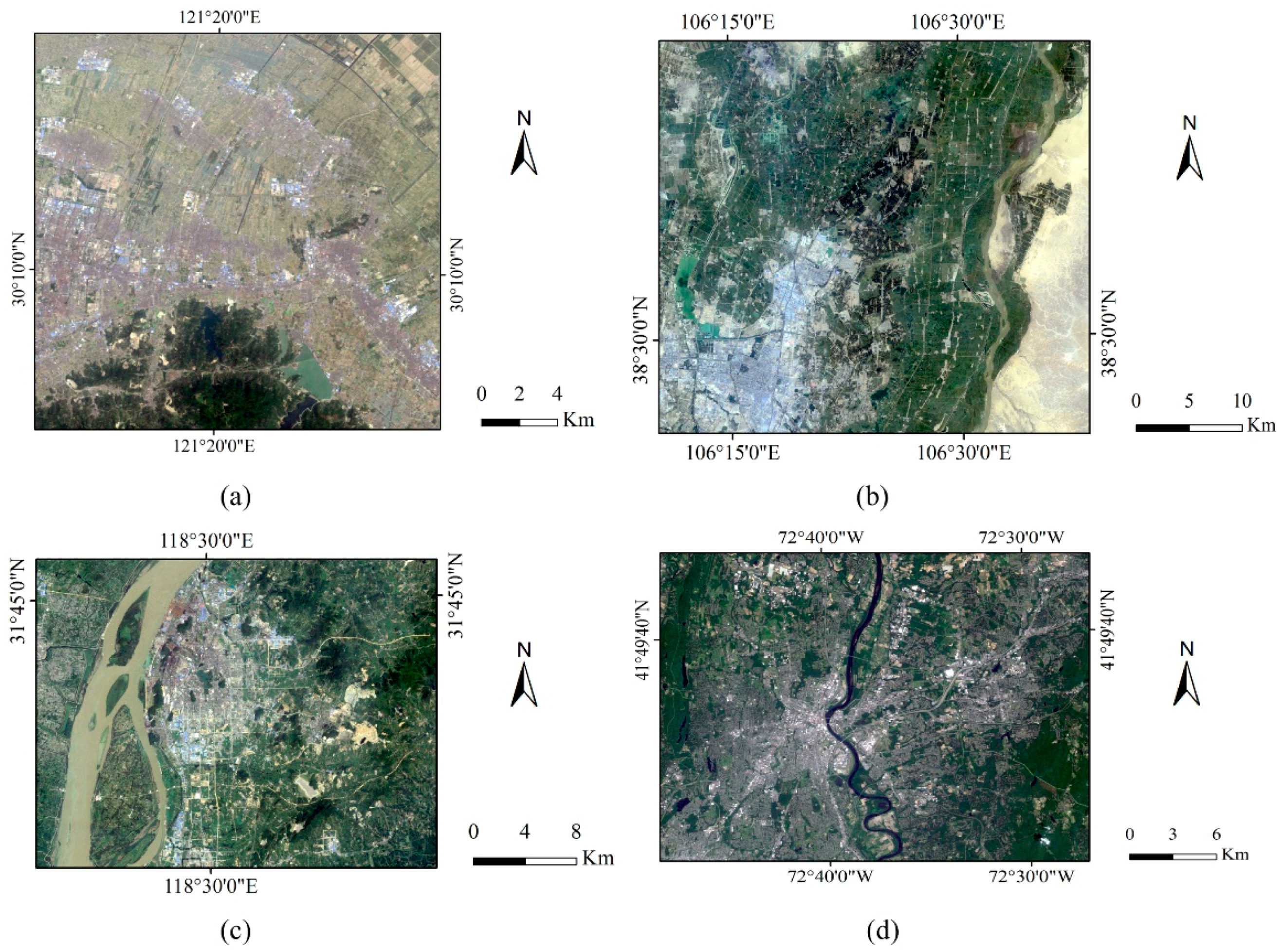
Four cases were chosen to be used in this research: (1) a part of Cixi city, Zhejiang, China, with upper left corner coordinates (121°13′47′′ E, 30°16′42″ N), recorded on 20 May 2011; (2) a part of Yinchuan city (including some area of nearby Shizuishan city), Ningxia, China, with upper left corner coordinates (106°10′33′′ E, 38°44′57″ N), recorded on 18 June 2011; (3) a part of Maanshan city, Anhui, China, with upper left corner coordinates (118°21′27″ E, 31°46′46″ N), recorded on 19 August 2010; (4) a part of Hartford, CT, USA, with upper left corner coordinates (72°48′4′′ W, 41°53′22″ N), recorded on 21 June 2011. Landsat 5 TM imagery was used in this study (see Figure 1). The images consist of seven spectral bands, with a medium spatial resolution of 30 m for Bands 1 to 5 and 7 and a spatial resolution of 120 m for Band 6. Therefore, Bands 1 to 5 and 7 were extracted for the classification purpose. The images were corrected for atmospheric and geometric distortion prior to use.
The image for the Cixi study area contains 722 columns by 702 rows of pixels and covers a variety of landscape elements, including urban areas, agricultural lands, lakes, rivers and mountains. Therefore, four major land use/cover classes were mapped, namely, built-up area, farmland, woodland and waterbody. The image for the Yinchuan study area, which includes a part of the adjacent Shizuishan city, contains 1354 columns by 1206 rows of pixels, with a complex landscape, including urban areas, agricultural lands, lakes, rivers, mountains and a large area of bare lands. Therefore, four major land use/cover classes were classified, namely, built-up area, farmland, bare land and waterbody. Bare land refers to the areas of bare soils or rocks with little vegetation cover. Generally, vegetation accounts for less than 15% of total cover. The image of the Maanshan study area contains 1047 columns by 800 rows of pixels. It has a more complex landscape, including urban areas, agricultural lands, rivers, mountains and residues of iron mines. So, five major land use/cover classes were mapped, namely, built-up area, farmland, woodland, bare land and waterbody. The image of the Hartford study area contains 995 columns by 809 rows of pixels. The landscape covers urban areas, agricultural lands, rivers, lakes and hills. Five major land use/cover classes were considered in classification, namely, high intensity development, low intensity development, farmland, woodland and waterbody. High intensity development refers to the areas with mainly constructed materials, such as urban cores. Low intensity development means the areas with a mixture of constructed materials and vegetation.
2.2. Expert-Interpreted Data
In this study, the SS-coMCRF model [42] was used to improve the accuracy of land use/cover classification by taking a pre-classified image as auxiliary data. To achieve this goal, pre-classification map data and expert-interpreted sample data were needed. For the purposes of land use/cover class identification and accuracy assessment, besides the Landsat images, some other reference data sources were needed for expert-interpretation of sample data (including sample data for validation). The other data sources we used in this study include Google earth imagery, fine resolution images from Terra server and satellite images from DigitalGlobe. The locations of sample data were randomly selected using ArcGIS. During the expert-interpretation process, unidentifiable pixels at selected locations were discarded and only identifiable pixels were interpreted as sample data. For each case study area, specific quantities of expert-interpreted sample data for post-classification and validation for each land use/cover class are given in Table 1. The total numbers of sample data (pixel class labels) used for post-classification for the four selected study areas are 1309 (0.258% of the total image pixels in the study area) for Cixi, 1428 (0.087% of the total image pixels in the study area) for Yinchuan, 1401 (0.167% of the total image pixels in the study area) for Maanshan and 1500 (0.186% of the total image pixels in the study area) for Hartford, respectively. As an example, Figure 2 shows the spatial distributions of the expert-interpreted sample data for post-classification and the expert-interpreted sample data for validation for the Yinchuan study area.
3. Methodology
3.1. General Procedure
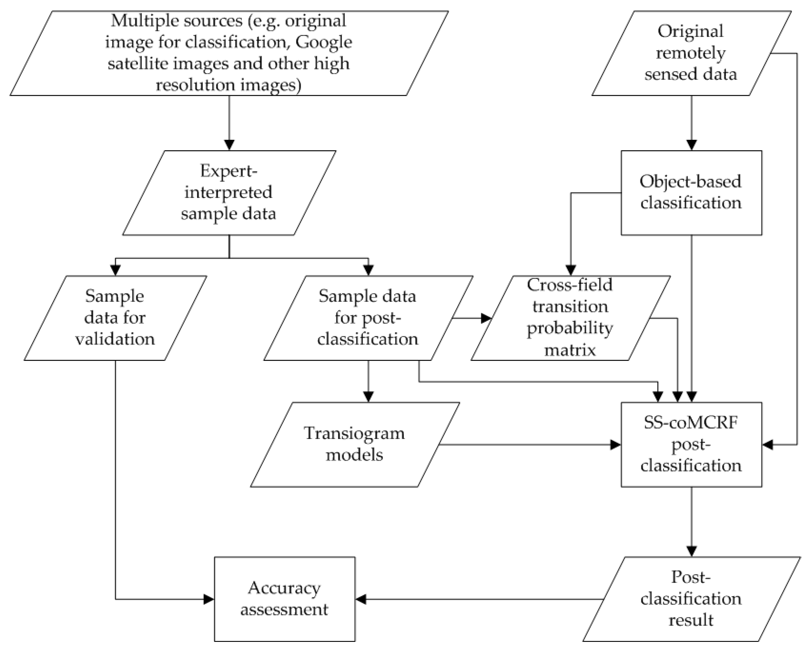
The flow chart of the MCRF post-classification methodology using the SS-coMCRF model was shown in Figure 3. An object-based classification method was employed to generate pre-classified image data. Sample data for post-classification simulation and accuracy assessment were expert-interpreted from multiple sources, such as the original image for classification, Google earth imagery, fine resolution images from Terra server and satellite images from DigitalGlobe. These sample data were split into two sets, one set for parameter estimation (i.e., estimation of transiogram models and cross-field transition probability matrix) and conditioning post-classification simulation and the other set for accuracy assessment (i.e., validation). The estimated parameters, together with pre-classified image data and the original remotely sensed image data, were inputs to the SS-coMCRF model for post-classification.
3.2. Spectral Similarity-Enhanced MCRF Co-Simulation Model
The core of the MCRF post-classification method is the coMCRF model [40] and the SS-coMCRF model [42], which incorporate all related data into a final classification through the post-classification operation to improve the accuracy of land use/cover classification. The coMCRF model is an extension of the MCRF model proposed by Li [43] in order to incorporate auxiliary data. The SS-coMCRF model is a modification of the coMCRF model in order to reduce the smoothing (or filtering) effect in post-classification, by incorporating spectral similarity measures based on the spectral values of the original remotely sensed image used in pre-classification. So, when the original remotely sensed image for land use/cover classification is available, the SS-coMCRF model can be used to reduce the loss of geometric features of some land use/cover classes in land use/cover post-classification.
Li [43] introduced the MCRF theory and the Markov chain geostatistical approach for simulating categorical fields. The MCRF model was derived by applying Bayes’ theorem [44] and sequential Bayesian updating to nearest data within a neighborhood and could be visualized as a probabilistic directed acyclic graph [40], thus being consistent with Bayesian Networks [44,45]. The conditional independence assumption for nearest data within a neighborhood, extended from a property of Pickard random fields, was used to simplify the MCRF full solution to a form that contains only transition probabilities [43,46]. The transiogram concept is one of the important components in this model. Li [47] introduced the transiogram as an accompanying spatial correlation measure of Markov chain geostatistics. The transiogram theoretically refers to a transition probability-lag function:
where represents the transition probability from class i to class j, Z(u) stands for a spatially stationary random variable at a specific location u and h, as a vector variable, refers to the separate distance between the two spatial points u and u + h. Visually, the transiogram is a transition probability-lag curve. While an auto-transiogram represents the autocorrelation of a land use/cover class, a cross-transiogram (i ≠ j) represents the cross-correlation of a pair of land use/cover classes. As transition probability, cross-transiograms are asymmetric and can be unidirectional.
Considering four nearest data and the quandrantal neighborhood (i.e., seeking one nearest datum from each quadrant sectoring the circular search area if there are nearest data in the quadrant), the SS-coMCRF model [42] can be given as:
where represents the location vector of a pixel, refers to the land use/cover class of the unobserved pixel at location ; to are the states of the four nearest neighbours around the unobserved location within a quadrantal neighbourhood; the left hand side of the equation is the posterior probability of class ; is a specific transition probability over the separation distance between locations and , which can be fetched from a corresponding transiogram model; represents the cross-field transition probability from class at the location in the primary field being simulated to class at the co-location in the covariate field (here the pre-classified image); and Spectrum here means the spectral data of the original remotely sensed image for pre-classification, which are used to calculate the spectral similarity-based constraining factor .
In above equation, the spectral similarity-based constraining factor S is calculated as:
where is the land use/cover class of pixel l; and are the spatial correlation measure (i.e., correlation coefficient) and Jaccard index of the spectral vectors (i.e., spectral values of different bands) and of pixel l and pixel k, respectively. See [42] for a detailed description of the SS-coMCRF model and the spectral similarity-based constraining factor.
3.3. Inputs and Outputs for the SS-coMCRF Model
In order to perform simulation using the SS-coMCRF model, cross-field transition probability matrix and transiogram models are required as input parameters, besides pre-classified image data, original remotely sensed image and expert-interpreted sample data. Transiogram models provide transition probability values at any needed lag values. Li and Zhang [48] proved that linear interpolation is more efficient than model fitting when samples are adequate and experimental transiograms are reliable. To take the advantage of the linear interpolation method, sufficient expert-interpreted sample data were selected to create reliable experimental transiograms in this study. Figure 4 shows a subset of transiogram models estimated from the expert-interpreted sample dataset for the Cixi case study. Table 2 shows the cross-field transition probability matrix, which expresses the cross correlations between classes of sample data and the pre-classified image data. One cross-field transition probability matrix is enough for a collocated co-simulation conditioned on one auxiliary data set and it can be calculated using the transitions from the selected sample points to their corresponding collocated points in the pre-classified image [40].
For each simulation case, the SS-coMCRF model generated one hundred of simulated realizations. Occurrence probabilities of land use classes at all pixels were estimated from the simulated realization maps. Based on the maximum probabilities, an optimal post-classification map was achieved for each case. After that, confusion matrix and Kappa coefficient were used to calculate the accuracy of each optimal post-classification map and pre-classified image using the corresponding validation data set.
3.4. Object-Based Classification
The object-based classification (OBC) approach was initially introduced in 1970s [49,50]. With the increased demand for OBC methods, many GIS software systems are available to use this kind of methods for classification. ENVI is one of the most commonly used software systems and it provides a K-Nearest Neighbor (KNN) object-based classification method. Due to its simplicity in implementation, clarity in theory and good performance in classification, KNN has become one of the most commonly used OBC methods. Therefore, the KNN method was employed for object-based classification in this study. The KNN object-based classification process has two steps: segmentation and classification. Segmentation is the way to partition a remote sensing image into different objects by merging pixels with similar attributes [51,52]. Segmentation is the most important part in object-based classification, because it can divide an image into homogeneous objects and ensure the classification results more accurate [50].
The KNN method was employed to segment an original remotely sensed image into land use segments and then chose a set of segments as training data based on different land use/cover classes to classify the segments. The parameters of segmentation were chosen based on visual inspection and researcher’s experience. Too many segments could increase processing time and were not necessary. In segment settings, the value of parameter Edge was set to 30 for detecting edges of features where objects of interest have sharp edges. Adjacent segments with similar spectral attributes can be merged. In this study, the value of Merge Level was set to 90 to merge over-segmented areas by using the Full Lambda Schedule algorithm. The value of Texture Kernel Size is the size (in pixels) of a moving box centered over each pixel in the image for computing texture attributes, which was set to 3. The resulting segments can clearly show boundaries of each land cover type. Because we conducted example-based classification, training data for classification were selected from segmented components. The number of object-based training samples was determined based on the researcher’s experience and 1000 object samples were randomly selected for each study case. Each training sample was chosen to contain only one land cover type. Based on the training samples and segments’ proximity to neighboring training regions, the KNN method assigned segments into different classes with the highest class confidence value.
4. Results and Discussions
4.1. Case 1
Figure 5 shows the pre-classification map and the corresponding MCRF post-classification map for the Cixi study area. Table 3 provides a comparison of classification accuracies between the pre-classification and the MCRF post-classification. The overall accuracy (OA) of the pre-classification map is 70.6%. However, the OA for the MCRF post-classification map is 84.7%. The overall improvement in land use/cover classification accuracy is 14.1%. The MCRF post-classification increased kappa coefficient from 0.552 to 0.762. In the pre-classification map, some built-up area pixels were misclassified into woodland and farmland. Due to the complexity of the landscape in this area, it is difficult to distinguish built-up area from woodland and farmland by purely using the KNN OBC method. After post-processing by MCRF co-simulation using the SS-coMCRF model, there are obvious increases in the producer’s accuracies of built-up area (increase from 65% to 87%), woodland (increase from 82% to 89%) and farmland (increase from 71% to 84%). In terms of the user’s accuracies, MCRF post-classification made improvements in the classification of built-up area (increase from 79% to 84%) and woodland (increase from 56% to 85%). However, the producer’s accuracy of waterbody decreased (from 57% to 50%). Considering that waterbody is a minor class, its accuracy assessment is not reliable and has little impact on the overall accuracy. Apparently, MCRF post-classification corrected many misclassified pixels and also reduced small noise features. A drawback is that some linear features (mainly roads or water channels here, pre-classified as linear objects of built-up area, woodland or waterbody), which were partially captured by the pre-classification, were lost in the MCRF post-classification map (Figure 5).
4.2. Case 2
Table 4 and Figure 6 present the pre-classification results by OBC and the corresponding post-classification results by SS-coMCRF for the Yinchuan study area. Compared with the pre-classification, the MCRF post-classification improved the OA by 5%. All classes have improvement in both producer’s accuracy and user’s accuracy. The MCRF post-classification increased kappa coefficient from 0.650 to 0.746. In the pre-classification map, bare land and built-up area were highly misclassified due to the confusion of their spectral values with farmland in the remotely sensed image, thus resulting in low producer’s accuracy for built-up area (69%) and bare land (68%). Meanwhile, low user’s accuracy (65%) also occurred for the built-up area in the pre-classification map due to the misclassification of some built-up area pixels into bare land and farmland. The MCRF post-classification operation changed this situation by correcting some misclassifications. Both producer’s accuracies and user’s accuracies of the four land use/cover classes were increased after MCRF post-classification. Similarly, most noise was removed in the post-classification map.
4.3. Case 3
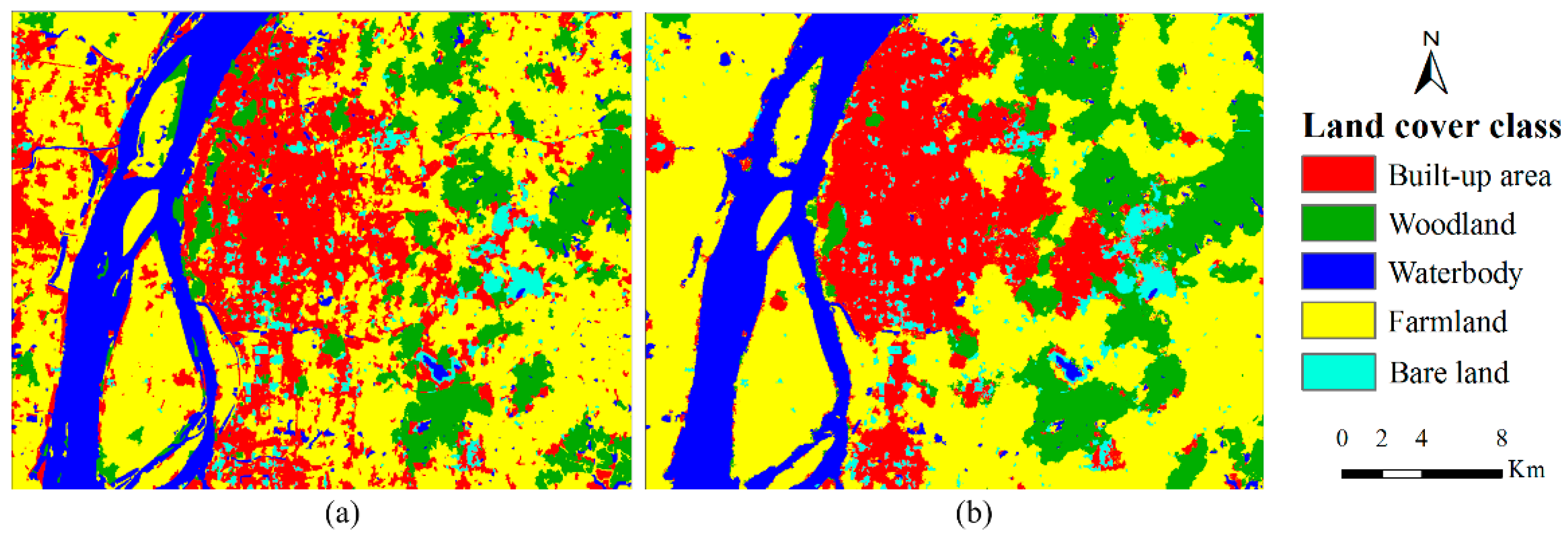
Results for Case 3 are provided in Figure 7 and Table 5. There are some residues of iron mines existing in the Maanshan city, which were classified as bare land. It is difficult to distinguish this kind of bare land from built-up area in this study area. That is why the pre-classification map has a relatively low producer’s accuracy for bare land (58%). Before post-classification, some bare land pixels were misclassified as built up area. After post-processing by the SS-coMCRF model, some misclassified bare land pixels were corrected. In the pre-classification map, because of spectral overlap of farmland with built-up area and woodland in the remotely sensed image, some pixels of built-up area and woodland were misclassified as farmland and similarly some pixels of farmland were misclassified as built-up area and woodland, thus resulting in relatively low producer’s accuracies (e.g., 63% for woodland and 70% for farmland). Because some waterbody areas were covered by water plants or other vegetation and those pixels were misclassified as farmland or woodland, the producer’s accuracy of waterbody was 85%. The MCRF post-classification operation changed this situation by correcting many misclassifications and consequently increased the OA and kappa coefficient by 11.8% and 0.165 (from 0.591 to 0.756), respectively. Specifically, post-classification improved the producer’s accuracies of built-up area, woodland, farmland and bare land by 9%, 13%, 13% and 19%, respectively and improved their user’s accuracies by 19%, 13%, 8% and 9%, respectively. The filtering effect of the MCRF post-classification method to noise was also clear.
4.4. Case 4
Hartford area has quite different landscape compared with other cases. The landscape was classified into five classes, including high intensity development, low intensity development, waterbody, farmland and woodland (Figure 8). Due to the complex landscape and the similarity between high intensity development and low intensity development, it is hard to distinguish these two classes. Therefore, many pixels of low intensity development were misclassified into high intensity development in the pre-classification map (Table 6). Therefore, high intensity development had a relatively low producer’s accuracy (69%). MCRF post-classification was able to correct some misclassified pixels and the producer’s accuracy of high intensity development was improved to 79%. Meanwhile, farmland was also pre-classified with very low accuracy, mainly due to its spectral overlap with developed area (i.e., both high and low intensity development here). MCRF post-classification improved the producer’s accuracy of farmland by 6%. The complex landscape and the local living style (i.e., residential houses are usually scattered in forest or farmland) resulted in high spectral confusion among land use/cover classes except for waterbody. That should be the major reason why the pre-classification OA was relatively low (74.6%), even if waterbody was pre-classified with high accuracy. MCRF post-classification improved the OA by 5.6%. The MCRF post-classification increased kappa coefficient from 0.633 to 0.711.
4.5. Discussions
In this study, the KNN method was used to represent the OBC approach as the pre-classifier. The MCRF post-classification method improves land use/cover classification accuracy by taking extra reliable information (expert-interpreted sample data from multiple sources and class spatial correlations estimated from the sample data) into a pre-classification that is previously performed by a conventional pre-classifier, usually based on spectral data of an original remotely sensed image. It does not matter which method or what kind of methods was used to perform the pre-classification. Depending on image quality, landscape complexity, classification scheme and pre-classification operation, pre-classification accuracy may be relatively high or low; consequently, corresponding accuracy improvement by post-classification may be different (small or large). What we aim to explore in this study is that whether the MCRF post-classification method (here the SS-coMCRF model) can improve the accuracy of the classification results generated by the OBC approach, by incorporating extra reliable information that can be easily available. Although the OBC approach is segment-based and the SS-coMCRF model is pixel-based, this does not mean that the SS-coMCRF model cannot be applied to the classification maps generated by an object-based method. The testing cases in this study showed that the pre-classification results generated by the KNN method is relatively low and considerable accuracy improvement (5% to 14% depending on different landscape cases) could be achieved and some noise (including misclassified small segments) also could be removed by the MCRF post-classification method.
There are no strict requirements on multiple source reference images for interpreting sample data, because what the MCRF post-classification method needs are just the land cover/use class labels of some sample pixels rather than the whole images. So, reference images can include the original image for pre-classification, images at the same or similar resolutions and images with finer resolutions. Fine-resolution images are better for discerning the land cover/use classes of sample pixels. While widely-used classifiers mainly use spectral values for classification, human eye can utilize much more information (such as context information) to discern the land cover/use class of a pixel in an image. So, human eye observation may discern the correct land cover/use classes of many pixels in an image, even if some of them cannot be correctly classified in a classification. As long as the landscape did not change substantially (i.e., the nature of land cover/use did not change) in the study area during the time change, reference images at similar time or even in different seasons are suitable to use. In case some pre-selected pixels cannot be clearly discerned, they can be discarded or alternative discernable pixels at nearby places can be used. If one source (e.g., Google satellite imagery) is not sufficient for interpreting sample data, more data sources may be used. So, this sample data expert-interpretation process seems ambiguous but in fact it is practical, given the availability of many online and offline data sources at the present time.
One limitation of the MCRF post-classification method is that interpreting the needed sample dataset from multiple sources for performing co-simulation may be somewhat time consuming. Currently, this is the main overhead for improving land use/cover classification quality using the MCRF approach. Although a higher density of expert-interpreted sample data may result in larger accuracy improvement in post-classification, the accuracy improvement rate quickly decreases with increasing density of sample data, as demonstrated by Li et al. [40] and Zhang et al. [42]. Therefore, the basic requirement for the number of expert-interpreted sample data is that they should suit the estimation of reliable parameters for MCRF co-simulation.
5. Conclusions
This study demonstrated that the MCRF post-classification method (i.e., the SS-coMCRF model here) is effective in improving the accuracies of object-based land use/cover classification maps (generated by the OBC approach using the KNN method in this study) from medium resolution remotely sensed images with different landscapes and classification schemes. Specifically, in our case studies, MCRF post-classification operation improved the OAs of object-based land use/cover classifications by 14.1%, 5%, 11.8% and 5.6% for the Cixi, Yinchuan, Maanshan and Hartford study areas, respectively. Such accuracy improvement should be attributed to the incorporation of the expert-interpreted sample data and spatial correlation information, which can help correct a large portion of misclassified pixels in segments in various landscape situations. Besides improving classification accuracy, MCRF post-classification also can effectively remove classification noise or minor sizes of patches to a large extent, thus improving recognition of land use/cover patterns. Therefore, the MCRF post-classification method is much more than a filter that aims to remove classification noise and minor sizes of patches, because the filtering methods do not incorporate extra credible information from other sources into the post-classification and thus they may not improve much or may even reduce classification accuracy (Zhang et al. 2016 [41]).
Acknowledgments
This research is partially supported by USA NSF grant No. 1414108. Authors have the sole responsibility to all of the viewpoints presented in the paper.
Author Contributions
Wenjie Wang Weidong Li, Chuanrong Zhang and Weixing Zhang contributed to the research design. Wenjie Wang Weidong Li and Chuanrong Zhang contributed to the writing of the paper. Wenjie Wang undertook analysis of data. Wenjie Wang, Weidong Li, Chuanrong Zhang and Weixing Zhang contributed to the revisions and critical reviews from the draft to the final stages of the paper.
Conflicts of Interest
The authors declare no conflict of interest.
References
- Weng, Q. A remote sensing—GIS evaluation of urban expansion and its impact on surface temperature in the Zhujiang Delta, China. Int. J. Remote Sens. 2001, 22, 1999–2014. [Google Scholar] [CrossRef]
- Hassan, Z.; Shabbir, R.; Ahmad, S.S.; Malik, A.H.; Aziz, N.; Butt, A.; Erum, S. Dynamics of land use and land cover change (LULCC) using geospatial techniques: A case study of Islamabad Pakistan. SpringerPlus 2016, 5, 812. [Google Scholar] [CrossRef] [PubMed]
- Dwivedi, R.S.; Sreenivas, K.; Ramana, K.V. Cover: Land-use/land-cover change analysis in part of Ethiopia using Landsat Thematic Mapper data. Int. J. Remote Sens. 2005, 26, 1285–1287. [Google Scholar] [CrossRef]
- Erle, E.; Pontius, R. Land-Use and Land-Cover Change: The Encycl Earth; Cleveland, C.J., Ed.; Environmental Information Coalition, National Council for Science and the Environment: Washington, DC, USA, 2007; Available online: http://www.ecotope.org/people/ellis/papers/ellis_eoe_lulcc_2007.pdf (accessed on 29 May 2017).
- Lu, D.; Mausel, P.; Brondízio, E.; Moran, E. Change detection techniques. Int. J. Remote Sens. 2004, 25, 2365–2407. [Google Scholar] [CrossRef]
- Chen, X.; Vierling, L.; Deering, D. A simple and effective radiometric correction method to improve landscape change detection across sensors and across time. Remote Sens. Environ. 2005, 98, 63–79. [Google Scholar] [CrossRef]
- Nuñez, M.N.; Ciapessoni, H.H.; Rolla, A.; Kalnay, E.; Cai, M. Impact of land use and precipitation changes on surface temperature trends in Argentina. J. Geophys. Res. 2008, 113, D06111. [Google Scholar] [CrossRef]
- Rahman, A.; Kumar, S.; Fazal, S.; Siddiqui, M.A. Assessment of land use/land cover change in the North-West District of Delhi using remote sensing and GIS techniques. J. Indian Soc. Remote Sens. 2012, 40, 689–697. [Google Scholar] [CrossRef]
- Foody, G.M. Remote sensing of tropical forest environments: Towards the monitoring of environmental resources for sustainable development. Int. J. Remote Sens. 2003, 24, 4035–4046. [Google Scholar] [CrossRef]
- Herold, M.; Scepan, J.; Clarke, K.C. The use of remote sensing and landscape metrics to describe structures and changes in urban land uses. Environ. Plan. A 2002, 34, 1443–1458. [Google Scholar] [CrossRef]
- Yuan, F.; Sawaya, K.E.; Loeffelholz, B.C.; Bauer, M.E. Land cover classification and change analysis of the Twin Cities (Minnesota) Metropolitan Area by multitemporal Landsat remote sensing. Remote Sens. Environ. 2005, 98, 317–328. [Google Scholar] [CrossRef]
- Srivastava, P.K.; Han, D.; Rico-Ramirez, M.A.; Bray, M.; Islam, T. Selection of classification techniques for land use/land cover change investigation. Adv. Space Res. 2012, 50, 1250–1265. [Google Scholar] [CrossRef]
- Guneroglu, A. Coastal changes and land use alteration on Northeastern part of Turkey. Ocean. Coast. Manag. 2015, 118, 225–233. [Google Scholar] [CrossRef]
- El-Asmar, H.M.; Taha, M.M.N.; El-Sorogy, A.S. Morphodynamic changes as an impact of human intervention at the Ras El-Bar-Damietta Harbor coast, NW Damietta Promontory, Nile Delta, Egypt. J. Afr. Earth Sci. 2016, 124, 323–339. [Google Scholar] [CrossRef]
- Rundquist, D.C.; Narumalani, S.; Narayanan, R.M. A review of wetlands remote sensing and defining new considerations. Remote Sens. Rev. 2001, 20, 207–226. [Google Scholar] [CrossRef]
- Zhang, S.Q.; Zhang, S.K.; Zhang, J.Y. A study on wetland classification model of remote sensing in the Sangjiang Plain. Chin. Geogr. Sci. 2000, 10, 68–73. [Google Scholar] [CrossRef]
- Butt, A.; Shabbir, R.; Ahmad, S.S.; Aziz, N. Land use change mapping and analysis using Remote Sensing and GIS: A case study of Simly watershed, Islamabad, Pakistan. Egypt. J. Remote Sens. Space Sci. 2015, 18, 251–259. [Google Scholar] [CrossRef]
- Guo, Q.; Kelly, M.; Gong, P.; Liu, D. An object-based classification approach in mapping tree mortality using high spatial resolution imagery. GISci. Remote Sens. 2007, 44, 24–47. [Google Scholar] [CrossRef]
- Li, C.; Wang, J.; Wang, L.; Hu, L.; Gong, P. Comparison of classification algorithms and training sample sizes in urban land classification with landsat thematic mapper imagery. Remote Sens. 2014, 6, 964–983. [Google Scholar] [CrossRef]
- Mas, J.-F. Monitoring land-cover changes: A comparison of change detection techniques. Int. J. Remote Sens. 1999, 20, 139–152. [Google Scholar] [CrossRef]
- Yang, X. Satellite monitoring of urban spatial growth in the Atlanta metropolitan area. Photogramm. Eng. Remote Sens. 2002, 68, 725–734. [Google Scholar] [CrossRef]
- Zhou, W.; Troy, A.; Grove, M. Object-based land cover classification and change analysis in the Baltimore metropolitan area using multitemporal high resolution remote sensing data. Sensors 2008, 8, 1613–1636. [Google Scholar] [CrossRef] [PubMed]
- Jawak, S.D.; Devliyal, P.; Luis, A.J. A comprehensive review on pixel oriented and object oriented methods for information extraction from remotely sensed satellite images with a special emphasis on cryospheric applications. Adv. Remote Sens. 2015, 4, 177–195. [Google Scholar] [CrossRef]
- Blaschke, T.; Lang, S.; Lorup, E.; Strobl, J.; Zeil, P. Object-oriented image processing in an integrated GIS/remote sensing environment and perspectives for environmental applications. Environ. Inf. Plan. Politics Public 2000, 2, 555–570. [Google Scholar]
- Blaschke, T. Object based image analysis for remote sensing. ISPRS J. Photogramm. Remote Sens. 2010, 65, 2–16. [Google Scholar] [CrossRef]
- Myint, S.W.; Giri, C.P.; Wang, L.; Zhu, Z.; Gillette, S.C. Identifying mangrove species and their surrounding land use and land cover classes using an object-oriented approach with a lacunarity spatial measure. GISci. Remote Sens. 2008, 45, 188–208. [Google Scholar] [CrossRef]
- Niemeyer, I.; Canty, M.J. Pixel-based and object-oriented change detection analysis using high-resolution imagery. In Proceedings of the 25th Symposium on Safeguards and Nuclear Material Management, Stockholm, Sweden, 13–15 May 2003; pp. 2133–2136. [Google Scholar]
- Chen, G.; Hay, G.J.; Carvalho, L.M.T.; Wulder, M.A. Object-based change detection. Int. J. Remote Sens. 2012, 33, 4434–4457. [Google Scholar] [CrossRef]
- Qian, Y.; Zhang, K.; Qiu, F. Spatial contextual noise removal for post classification smoothing of remotely sensed images. In Proceedings of the 2005 ACM Symposium on Applied Computing, Santa Fe, New Mexico, 13–17 March 2005; pp. 524–528. [Google Scholar] [CrossRef]
- Gong, P.; Howarth, P.J. Frequency-based contextual classification and gray-level vector reduction for land-use identification. Photogramm. Eng. Remote Sens. 1992, 58, 423–437. [Google Scholar]
- Gallego, F.J. Remote sensing and land cover area estimation. Int. J. Remote Sens. 2004, 25, 3019–3047. [Google Scholar] [CrossRef]
- Lu, D.; Weng, Q. A survey of image classification methods and techniques for improving classification performance. Int. J. Remote Sens. 2007, 28, 823–870. [Google Scholar] [CrossRef]
- Manandhar, R.; Odeh, I.O.A.; Ancev, T. Improving the accuracy of land use and land cover classification of Landsat data using post-classification enhancement. Remote Sens. 2009, 1, 330–344. [Google Scholar] [CrossRef]
- Stow, D.A.; Collins, D.; McKinsey, D. Land use change detection based on multi-date imagery from different satellite sensor systems. Geocarto Int. 1990, 5, 3–12. [Google Scholar] [CrossRef]
- Foody, G.M. Status of land cover classification accuracy assessment. Remote Sens. Environ. 2002, 80, 185–201. [Google Scholar] [CrossRef]
- Wilkinson, G.G. Results and implications of a study of fifteen years of satellite image classification experiments. IEEE Trans. Geosci. Remote Sens. 2005, 43, 433–440. [Google Scholar] [CrossRef]
- Blaes, X.; Vanhalle, L.; Defourny, P. Efficiency of crop identification based on optical and SAR image time series. Remote Sens. Environ. 2005, 96, 352–365. [Google Scholar] [CrossRef]
- Recio, J.; Hermosilla, T.; Ruiz, L.; Fdez-Sarría, A. Analysis of the addition of qualitative ancillary data on parcel-based image classification. Int. Arch. Photogramm. Remote Sens. Spat. Inf. Sci. 2009, 38, 1–4. [Google Scholar]
- Lawrence, R.L.; Wrlght, A. Rule-based classification systems using classification and regression tree (CART) analysis. Photogramm. Eng. Remote Sens. 2001, 67, 1137–1142. [Google Scholar] [CrossRef]
- Li, W.; Zhang, C.; Willig, M.R.; Dey, D.K.; Wang, G.; You, L. Bayesian Markov chain random field cosimulation for improving land cover classification accuracy. Math. Geosci. 2015, 47, 123–148. [Google Scholar] [CrossRef]
- Zhang, W.; Li, W.; Zhang, C. Land cover post-classifications by Markov chain geostatistical cosimulation based on pre-classifications by different conventional classifiers. Int. J. Remote Sens. 2016, 37, 926–949. [Google Scholar] [CrossRef]
- Zhang, W.; Li, W.; Zhang, C.; Li, X. Incorporating spectral similarity into Markov chain geostatistical cosimulation for reducing smoothing effect in land cover postclassification. IEEE J. Sel. Top. Appl. Earth Obs. Remote Sens. 2017, 10, 1082–1095. [Google Scholar] [CrossRef]
- Li, W. Markov chain random fields for estimation of categorical variables. Math. Geol. 2007, 39, 321–335. [Google Scholar] [CrossRef]
- Bayes, M.; Price, M. An essay towards solving a problem in the doctrine of chances. By the Late Rev. Mr. Bayes, F. R. S. Communicated by Mr. Price, in a Letter to John Canton, A. M. F. R. S. Philos. Trans. R. Soc. Lond. 1763, 53, 370–418. [Google Scholar] [CrossRef]
- Jaffray, J. Bayesian updating and belief functions. In Classic Works of the Dempster-Shafer Theory of Belief Functions; Springer: Berlin/Heidelberg, Germany, 2008; Volume 219, pp. 555–576. [Google Scholar]
- Li, W.; Zhang, C. A single-chain-based multidimensional Markov chain model for subsurface characterization. Environ. Ecol. Stat. 2008, 15, 157–174. [Google Scholar] [CrossRef]
- Li, W. Transiograms for characterizing spatial variability of soil classes. Soil Sci. Soc. Am. J. 2007, 71, 881–893. [Google Scholar] [CrossRef]
- Li, W.; Zhang, C. Linear interpolation and joint model fitting of experimental transiograms for Markov chain simulation of categorical spatial variables. Int. J. Geogr. Inf. Sci. 2010, 24, 821–839. [Google Scholar] [CrossRef]
- De Kok, R.; Schneider, T.; Baatz, M. Object based image analysis of high resolution data in the alpine forest area. In Proceedings of the Joint Workshop for ISPRS WG I/1, I/3 AND IV/4, Sensors and Mappinhg from Space, Hanover, Germany, 27–30 September 1999; pp. 27–30. [Google Scholar]
- Yan, G.; Mas, J.-F.; Maathuis, B.H.P.; Xiangmin, Z.; Van Dijk, P.M. Comparison of pixel-based and object-oriented image classification approaches—A case study in a coal fire area, Wuda, Inner Mongolia, China. Int. J. Remote Sens. 2006, 27, 4039–4055. [Google Scholar] [CrossRef]
- Wolf, R. Redefining the concept of insulation. Tech. Text. Int. 1996, 5, 18–20. [Google Scholar] [CrossRef]
- Bhaskaran, S.; Paramananda, S.; Ramnarayan, M. Per-pixel and object-oriented classification methods for mapping urban features using Ikonos satellite data. Appl. Geogr. 2010, 30, 650–665. [Google Scholar] [CrossRef]
Figure 1.
Landsat 5 images used in case studies: (a) a part of Cixi city, Zhejiang, China; (b) a part of Yinchuan city, Ningxia, China; (c) a part of Maanshan city, Anhui, China; (d) a part of Hartford, CT, USA.
Figure 1.
Landsat 5 images used in case studies: (a) a part of Cixi city, Zhejiang, China; (b) a part of Yinchuan city, Ningxia, China; (c) a part of Maanshan city, Anhui, China; (d) a part of Hartford, CT, USA.

Figure 2.
Expert-interpreted land use/cover sample data for the study area in Yinchuan: (a) a subset of 1428 sample data for MCRF co-simulation (0.087% of the total image pixels); and (b) a subset of 518 sample data for validation.
Figure 2.
Expert-interpreted land use/cover sample data for the study area in Yinchuan: (a) a subset of 1428 sample data for MCRF co-simulation (0.087% of the total image pixels); and (b) a subset of 518 sample data for validation.
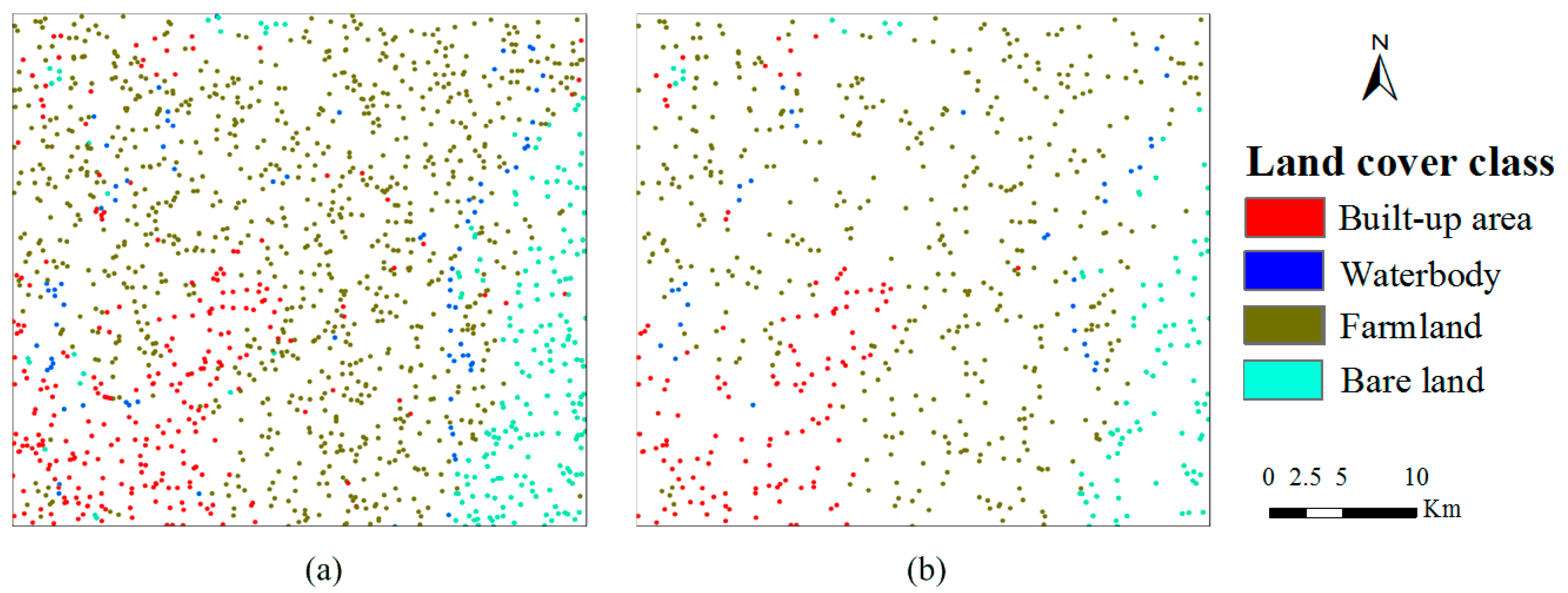
Figure 3.
The flow chart of the MCRF post-classification methodology using the SS-coMCRF model.

Figure 4.
A subset of transiogram models estimated from the expert-interpreted sample data for the Cixi case study. P(1-1) denotes the auto transition probability of built-up area. P(1-2) denotes the cross-transition probability from built-up area to woodland. P(1-3) denotes the cross-transition probability from built-up area to waterbody. P(1-4) denotes the cross-transition probability from built-up area to farmland. Lag is the separate distance between a pair of data points.
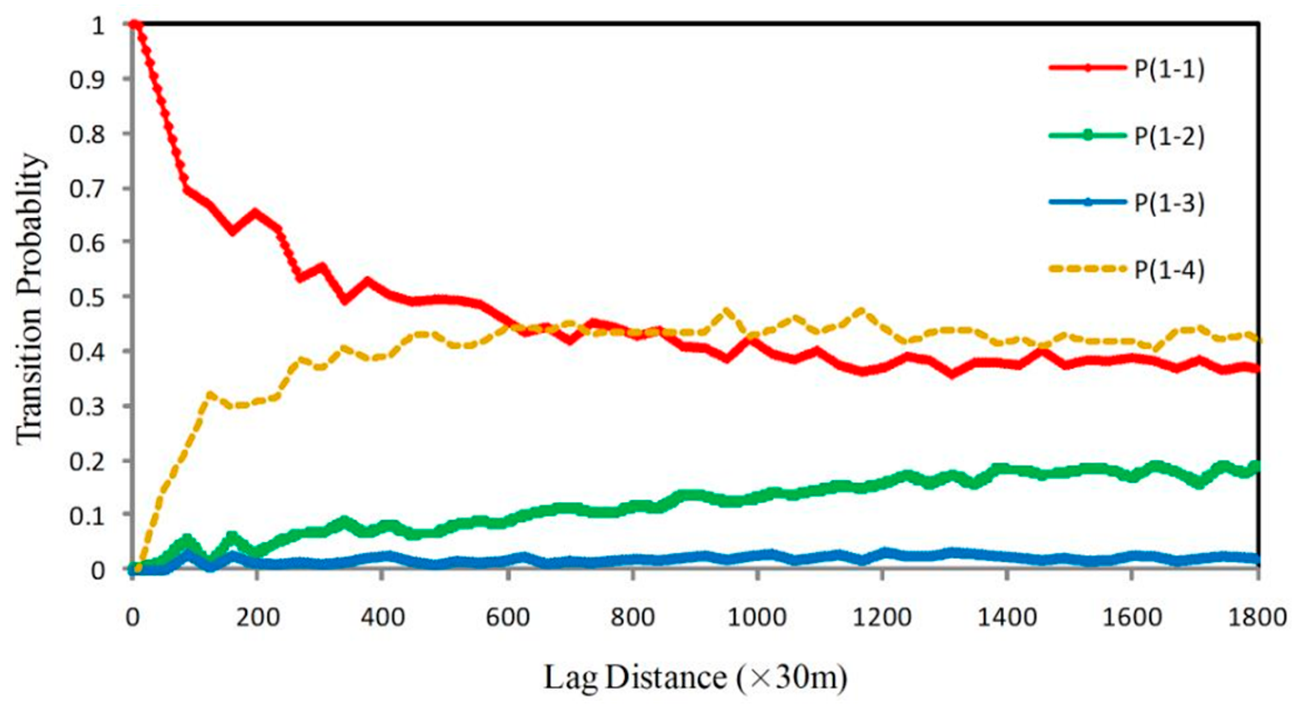
Figure 5.
Land use/cover classification results for the Cixi study area: (a) pre-classification map; (b) MCRF post-classification map.
Figure 5.
Land use/cover classification results for the Cixi study area: (a) pre-classification map; (b) MCRF post-classification map.
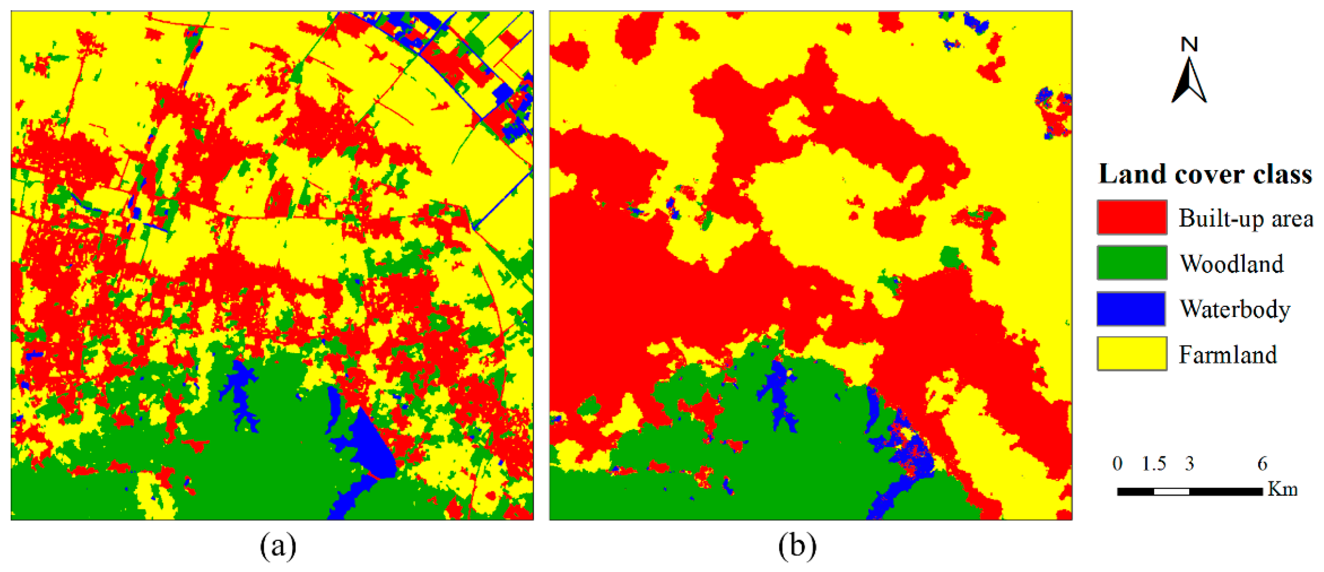
Figure 6.
Land use/cover classification results for the Yinchuan study area: (a) pre-classification map; (b) MCRF post-classification.
Figure 6.
Land use/cover classification results for the Yinchuan study area: (a) pre-classification map; (b) MCRF post-classification.
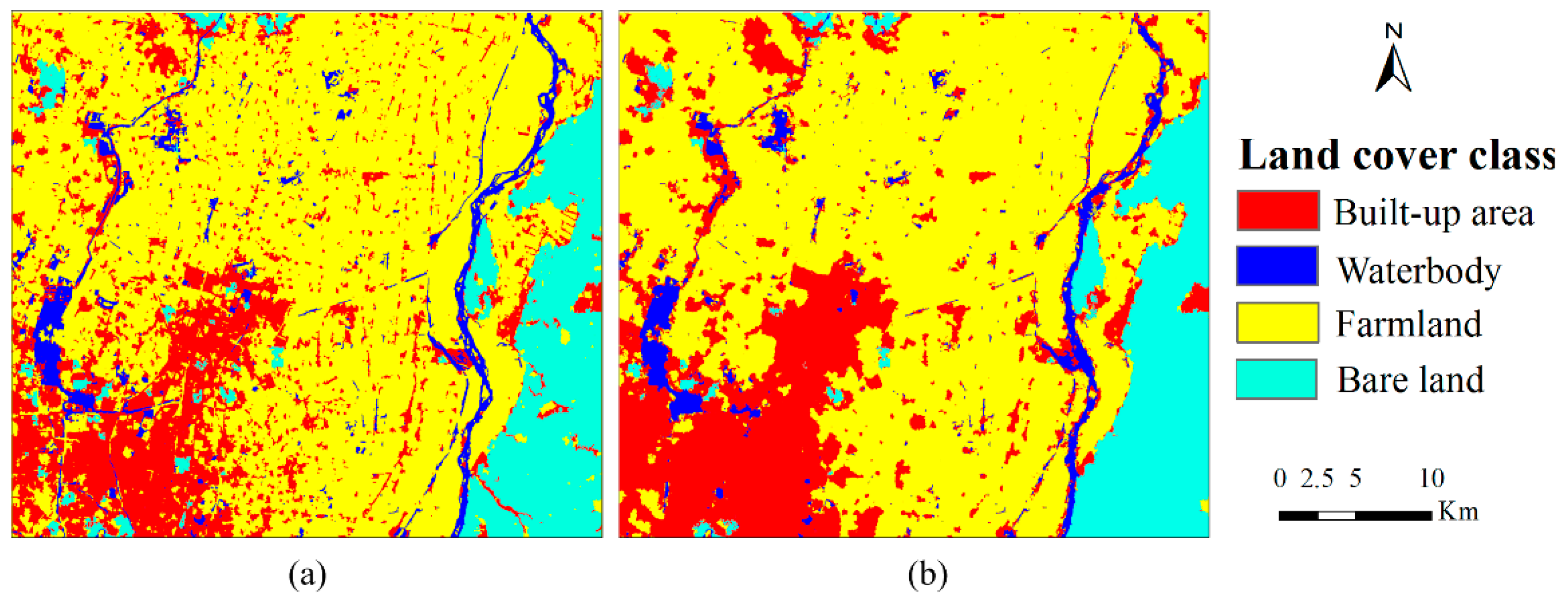
Figure 7.
Land use/cover classification results for the Maanshan study area: (a) pre-classification map; (b) MCRF post-classification map.
Figure 7.
Land use/cover classification results for the Maanshan study area: (a) pre-classification map; (b) MCRF post-classification map.

Figure 8.
Land use/cover classification results for the Hartford study area: (a) pre-classification map; (b) MCRF post-classification.
Figure 8.
Land use/cover classification results for the Hartford study area: (a) pre-classification map; (b) MCRF post-classification.


Table 1.
Quantities of expert-interpreted sample datasets and validation data sets for the four case studies.
Table 1.
Quantities of expert-interpreted sample datasets and validation data sets for the four case studies.
| Cixi City | Expert-Interpreted Sample Data (Pixels) | Validation Data (Pixels) | Yinchuan City | Expert-Interpreted Sample Data (Pixels) | Validation Data (Pixels) |
| Built-up area | 512 | 147 | Built-up area | 338 | 121 |
| Woodland | 150 | 71 | Farmland | 882 | 324 |
| Waterbody | 31 | 14 | Waterbody | 59 | 20 |
| Farmland | 616 | 193 | Bare land | 149 | 53 |
| Total | 1309 | 425 | Total | 1428 | 518 |
| Maanshan City | Expert-Interpreted Sample Data (Pixels) | Validation Data (Pixels) | Hartford City | Expert-Interpreted Sample Data (Pixels) | Validation Data (Pixels) |
| Built-up area | 347 | 134 | High intensity development | 299 | 94 |
| Woodland | 208 | 80 | Farmland | 429 | 167 |
| Waterbody | 80 | 67 | Waterbody | 36 | 14 |
| Farmland | 699 | 269 | Bare land | 114 | 30 |
| Bare land | 67 | 26 | Low intensity development | 622 | 277 |
| Total | 1401 | 576 | Total | 1500 | 582 |
Table 2.
Cross-field transition probability matrix from classes of the expert-interpreted dataset to classes of the pre-classified data by the object-based classification for the Cixi case study.
Table 2.
Cross-field transition probability matrix from classes of the expert-interpreted dataset to classes of the pre-classified data by the object-based classification for the Cixi case study.
| Cross-Field Transition Probability | |||||
|---|---|---|---|---|---|
| Pre-Classification Data | |||||
| Class ** | C1 | C2 | C3 | C4 | |
| Expert-interpreted sample data | C1 | 0.602 | 0.077 | 0.005 | 0.317 |
| C2 | 0 | 0.932 | 0 | 0.068 | |
| C3 | 0.231 | 0.231 | 0.538 | 0 | |
| C4 | 0.086 | 0.126 | 0.007 | 0.781 | |
** C1—Built-up area; C2—Woodland; C3—Waterbody; C4—Farmland.
Table 3.
Accuracy assessment for pre-classification and corresponding post-classification for the Cixi study area.
Table 3.
Accuracy assessment for pre-classification and corresponding post-classification for the Cixi study area.
| Object-Based Pre-Classification | MCRF Post-Classification | |||||||||||
|---|---|---|---|---|---|---|---|---|---|---|---|---|
| Class ** | C1 | C2 | C3 | C4 | Total | User’s Accuracy (%) | C1 | C2 | C3 | C4 | Total | User’s Accuracy (%) |
| C1 | 96 | 2 | 1 | 22 | 121 | 79 | 128 | 2 | 1 | 22 | 153 | 84 |
| C2 | 12 | 58 | 2 | 31 | 109 | 56 | 2 | 63 | 0 | 9 | 80 | 85 |
| C3 | 0 | 0 | 8 | 2 | 10 | 80 | 0 | 0 | 7 | 0 | 7 | 100 |
| C4 | 39 | 11 | 3 | 138 | 185 | 72 | 17 | 6 | 6 | 162 | 185 | 85 |
| Total | 147 | 71 | 14 | 193 | 425 | 147 | 71 | 14 | 193 | 425 | ||
| Producer’s accuracy (%) | 65 | 82 | 57 | 71 | 70.6 | 87 | 89 | 50 | 84 | 84.7 | ||
** C1—Built-up area; C2—Woodland; C3—Waterbody; C4—Farmland.
Table 4.
Accuracy assessment for pre-classification and corresponding post-classification for the Yinchuan study area.
Table 4.
Accuracy assessment for pre-classification and corresponding post-classification for the Yinchuan study area.
| Object-Based Classification | MCRF Post-Classification | |||||||||||
|---|---|---|---|---|---|---|---|---|---|---|---|---|
| Class ** | C1 | C2 | C3 | C4 | Total | User’s Accuracy (%) | C1 | C2 | C3 | C4 | Total | User’s Accuracy (%) |
| C1 | 83 | 33 | 0 | 11 | 128 | 65 | 97 | 26 | 0 | 9 | 132 | 73 |
| C2 | 32 | 287 | 5 | 6 | 330 | 87 | 21 | 294 | 3 | 5 | 323 | 91 |
| C3 | 0 | 2 | 15 | 0 | 17 | 88 | 0 | 2 | 17 | 0 | 19 | 89 |
| C4 | 6 | 2 | 0 | 36 | 44 | 82 | 3 | 2 | 0 | 39 | 44 | 89 |
| Total | 121 | 324 | 20 | 53 | 518 | 121 | 324 | 20 | 53 | 518 | ||
| Producer’s accuracy (%) | 69 | 89 | 75 | 68 | 81.3 | 80 | 91 | 85 | 74 | 86.3 | ||
** C1—Built-up area; C2—Farmland; C3—Waterbody; C4—Bare land.
Table 5.
Accuracy assessment for pre-classification and corresponding SS-coMCRF post-classification for the Maanshan study area.
Table 5.
Accuracy assessment for pre-classification and corresponding SS-coMCRF post-classification for the Maanshan study area.
| Object-Based Pre-Classification | MCRF Post-Classification | |||||||||||||
|---|---|---|---|---|---|---|---|---|---|---|---|---|---|---|
| Class ** | C1 | C2 | C3 | C4 | C5 | Total | User’s Accuracy (%) | C1 | C2 | C3 | C4 | C5 | Total | User’s Accuracy (%) |
| C1 | 101 | 9 | 0 | 51 | 7 | 168 | 60 | 112 | 2 | 0 | 23 | 4 | 141 | 79 |
| C2 | 4 | 50 | 5 | 23 | 0 | 82 | 61 | 1 | 61 | 3 | 16 | 1 | 82 | 74 |
| C3 | 0 | 3 | 57 | 0 | 2 | 66 | 92 | 0 | 2 | 62 | 1 | 0 | 65 | 95 |
| C4 | 28 | 18 | 4 | 187 | 2 | 235 | 78 | 19 | 15 | 1 | 223 | 1 | 259 | 86 |
| C5 | 1 | 0 | 1 | 8 | 15 | 25 | 60 | 2 | 0 | 1 | 6 | 20 | 29 | 69 |
| Total | 134 | 80 | 67 | 269 | 26 | 576 | 134 | 80 | 67 | 269 | 26 | 576 | ||
| Producer’s accuracy (%) | 75 | 63 | 85 | 70 | 58 | 71.2 | 84 | 76 | 92 | 83 | 77 | 83.0 | ||
** C1—Built-up area; C2—Woodland; C3—Waterbody; C4—Farmland; C5—Bare land.
Table 6.
Accuracy assessment for pre-classification and corresponding post-classification for the Hartford study area.
Table 6.
Accuracy assessment for pre-classification and corresponding post-classification for the Hartford study area.
| Object-Based Pre-Classification | MCRF Post-Classification | |||||||||||||
|---|---|---|---|---|---|---|---|---|---|---|---|---|---|---|
| Class ** | C1 | C2 | C3 | C4 | C5 | Total | User’s Accuracy (%) | C1 | C2 | C3 | C4 | C5 | Total | User’s Accuracy (%) |
| C1 | 65 | 17 | 0 | 2 | 43 | 127 | 51 | 74 | 12 | 0 | 1 | 33 | 120 | 62 |
| C2 | 6 | 140 | 0 | 3 | 31 | 180 | 78 | 5 | 147 | 0 | 3 | 27 | 182 | 81 |
| C3 | 0 | 0 | 12 | 0 | 0 | 12 | 100 | 0 | 0 | 12 | 0 | 0 | 12 | 100 |
| C4 | 11 | 6 | 0 | 21 | 7 | 45 | 46 | 5 | 4 | 0 | 22 | 5 | 36 | 61 |
| C5 | 12 | 4 | 2 | 4 | 196 | 218 | 90 | 10 | 4 | 2 | 4 | 212 | 232 | 91 |
| Total | 94 | 167 | 14 | 30 | 277 | 582 | 94 | 167 | 14 | 30 | 277 | 582 | ||
| Producer’s accuracy (%) | 69 | 84 | 86 | 70 | 71 | 74.6 | 79 | 88 | 86 | 73 | 77 | 80.2 | ||
** C1—High intensity development; C2—Woodland; C3—Waterbody; C4—Farmland; C5—Low intensity development.
© 2018 by the authors. Licensee MDPI, Basel, Switzerland. This article is an open access article distributed under the terms and conditions of the Creative Commons Attribution (CC BY) license (http://creativecommons.org/licenses/by/4.0/).
Share and Cite
MDPI and ACS Style
Wang, W.; Li, W.; Zhang, C.; Zhang, W. Improving Object-Based Land Use/Cover Classification from Medium Resolution Imagery by Markov Chain Geostatistical Post-Classification. Land 2018, 7, 31. https://doi.org/10.3390/land7010031
AMA Style
Wang W, Li W, Zhang C, Zhang W. Improving Object-Based Land Use/Cover Classification from Medium Resolution Imagery by Markov Chain Geostatistical Post-Classification. Land. 2018; 7(1):31. https://doi.org/10.3390/land7010031
Chicago/Turabian StyleWang, Wenjie, Weidong Li, Chuanrong Zhang, and Weixing Zhang. 2018. "Improving Object-Based Land Use/Cover Classification from Medium Resolution Imagery by Markov Chain Geostatistical Post-Classification" Land 7, no. 1: 31. https://doi.org/10.3390/land7010031
Note that from the first issue of 2016, this journal uses article numbers instead of page numbers. See further details here.