Tetraquark Spectroscopy: A Symmetry Analysis

Abstract

We present a detailed analysis of the symmetry properties of a four-quark wave function and its solution by means of a variational approach for simple Hamiltonians. We discuss several examples in the light and heavy-light meson sector.

1. Introduction

The potentiality of the quark model for hadron physics in the low-energy regime became first manifest when it was used to classify the known hadron states. Describing hadrons as $q\overline{q}$ or $qqq$ configurations, their quantum numbers were correctly explained. This assignment was based on the comment by Gell-Mann [1] Ge64 introducing the notion of quark: “It is assuming that the lowest baryon configuration ($qqq$) gives just the representations 1, 8 and 10, that have been observed, while the lowest meson configuration ($q\overline{q}$) similarly gives just 1 and 8”. Since then, it has been assumed that these are the only two configurations involved in the description of physical hadrons. However, color confinement is also compatible with other multiquark structures like the tetraquark $qq\overline{q}\overline{q}$ first introduced by Jaffe [2]. During the last two decades there appeared a number of experimental data that are hardly accommodated in the traditional scheme defined by Gell-Mann.

One of the first scenarios where the existence of bound multiquarks was proposed was a system composed of two light quarks and two heavy antiquarks ($nn\overline{Q}\overline{Q}$). These objects are called heavy-light tetraquarks due to the similarity of their structure with the heavy-light mesons ($n\overline{Q}$). Although they may be experimentally difficult to produce and also to detect [3] it has been argued that for sufficiently large heavy quark mass the tetraquark should be bound [4,5]. The stability of a heavy-light tetraquark relies on the heavy quark mass. The heavier the quark the more effective the short-range Coulomb attraction to generate binding, in such a way that it could play a decisive role to bind the system. Moreover the $\overline{Q}\overline{Q}$ pair brings a small kinetic energy into the system contributing to stabilize it.

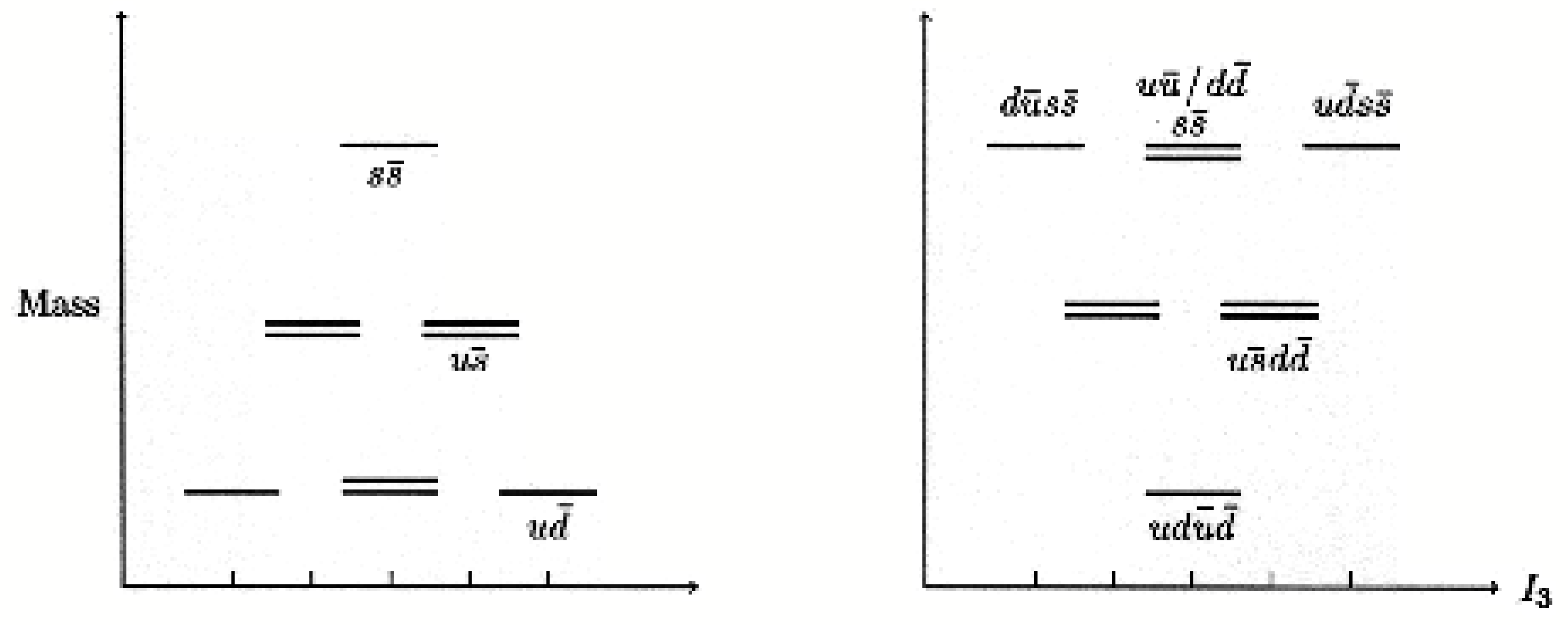
Another interesting scenario where tetraquarks may be present corresponds to the scalar mesons, $J^{PC}=0^{++}$. To obtain a positive parity state from a $q\overline{q}$ pair one needs at least one unit of orbital angular momentum. Apparently this costs an energy around 0.5 GeV1, making the lightest theoretical scalar states to be around 1.3 GeV, far from their experimental error bars. However, a $qq\overline{q}\overline{q}$ state can couple to $J^{PC}=0^{++}$ without orbital excitation and, as a consequence, they could coexist and mix with $q\overline{q}$ states in this energy region. Furthermore, the color and spin dependent interaction arising from the one-gluon exchange, favors states where quarks and antiquarks are separately antisymmetric in flavor. Thus, the energetically favored flavor configuration for $qq\overline{q}\overline{q}$ is $[{(qq)}_{\overline{3}}{(\overline{q}\overline{q})}_3]$, a flavor nonet, having the lightest multiplet spin 0. The most striking feature of a scalar $qq\overline{q}\overline{q}$ nonet in comparison with a $q\overline{q}$ nonet is a reversed mass spectrum (see Figure 1). One can see a degenerate isosinglet and isotriplet at the top of the multiplet, an isosinglet at the bottom, and a strange isodoublet in between. The resemblance to the experimental structure of the light scalar mesons is striking.

Four-quark states could also play an important role in the charm sector. Since 2003 there have been discovered several open-charm mesons: the $D_{sJ}^{\ast }(2317)$, the $D_{sJ}(2460)$, and the $D_0^{\ast }(2308)$. In the subsequent years several new states joined this exclusive group either in the open-charm sector: the $D_{sJ}(2860)$, or in the charmonium spectra: the $X(3872)$, the $X(3940)$, the $Y(3940)$, the $Z(3940)$, the $Y(4260)$, and the $Z(4430)$ among others [6]. It seems nowadays unavoidable to resort to higher order Fock space components to tame the bewildering landscape arising with these new findings. Four-quark components, either pure or mixed with $q\overline{q}$ states, constitute a natural explanation for the proliferation of new meson states [7,8,9]. They would also account for the possible existence of exotic mesons as could be stable $cc\overline{n}\overline{n}$ states, the topic for discussion since the early 1980s [10,11].

All these scenarios suggest the study of $qq\overline{q}\overline{q}$ structures and their possible mixing with the $q\overline{q}$ systems to understand the role played by multiquarks in the hadron spectra. The manuscript is organized as follows. In Section 2. the variational formalism necessary to evaluate four-quark states is discussed in detail with special emphasis on the symmetry properties. In Section 3. the way to exploit discrete symmetries to determine the four-quark decay threshold is discussed. In Section 4. the formalism to evaluate four-quark state probabilities is sketched. In Section 5. we discuss some examples of four-quark states calculated using this formalism. Finally, we summarize in Section 6. our conclusions.

2. Four-Quark Spectra

2.1. Solving the four-body system

The four-quark ($qq\overline{q}\overline{q}$) problem will be addressed by means of the variational method, specially suited for studying low-lying states. The nonrelativistic Hamiltonian will be given by

$$H=\sum _{i=1}^4\left(m_i+\frac{{\overrightarrow{p}}_i^2}{2m_i}\right)+\sum _{i<j=1}^{4}V({\overrightarrow{r}}_{ij})$$

(1)

where the potential $V({\overrightarrow{r}}_{ij})$ corresponds to an arbitrary two-body interaction. The extension of this formalism to consider many-body interactions is discussed in [12,13].

The variational wave function must include all possible flavor-spin-color channels contributing to a given configuration. For each channel s, the wave function will be the tensor product of a color ($\left|C_{s_1}\right.〉$), spin ($\left|S_{s_2}\right.〉$), flavor ($\left|F_{s_3}\right.〉$), and radial ($\left|R_{s_4}\right.〉$) component,

$$\left|{\varphi }_s\right.〉=\left|C_{s_1}\right.〉\otimes \left|S_{s_2}\right.〉\otimes \left|F_{s_3}\right.〉\otimes \left|R_{s_4}\right.〉$$

(2)

where $s\equiv \{s_1,s_2,s_3,s_4\}$. The procedure to construct the wave function will be detailed later on. Once the spin, color and flavor parts are integrated out the coefficients of the radial wave function are obtained by solving the system of linear equations

$$\sum _{s^{\prime }s}\sum _i{\beta }_{s_4}^{(i)}[\langle R_{s_4^{\prime }}^{(j)}\left|H\right|R_{s_4}^{(i)}\rangle -E\langle R_{s_4^{\prime }}^{(j)}|R_{s_4}^{(i)}\rangle {\delta }_{s,s^{\prime }}]=0\forall j$$

(3)

where the eigenvalues are obtained by a minimization procedure.

2.2. Four-body wave function

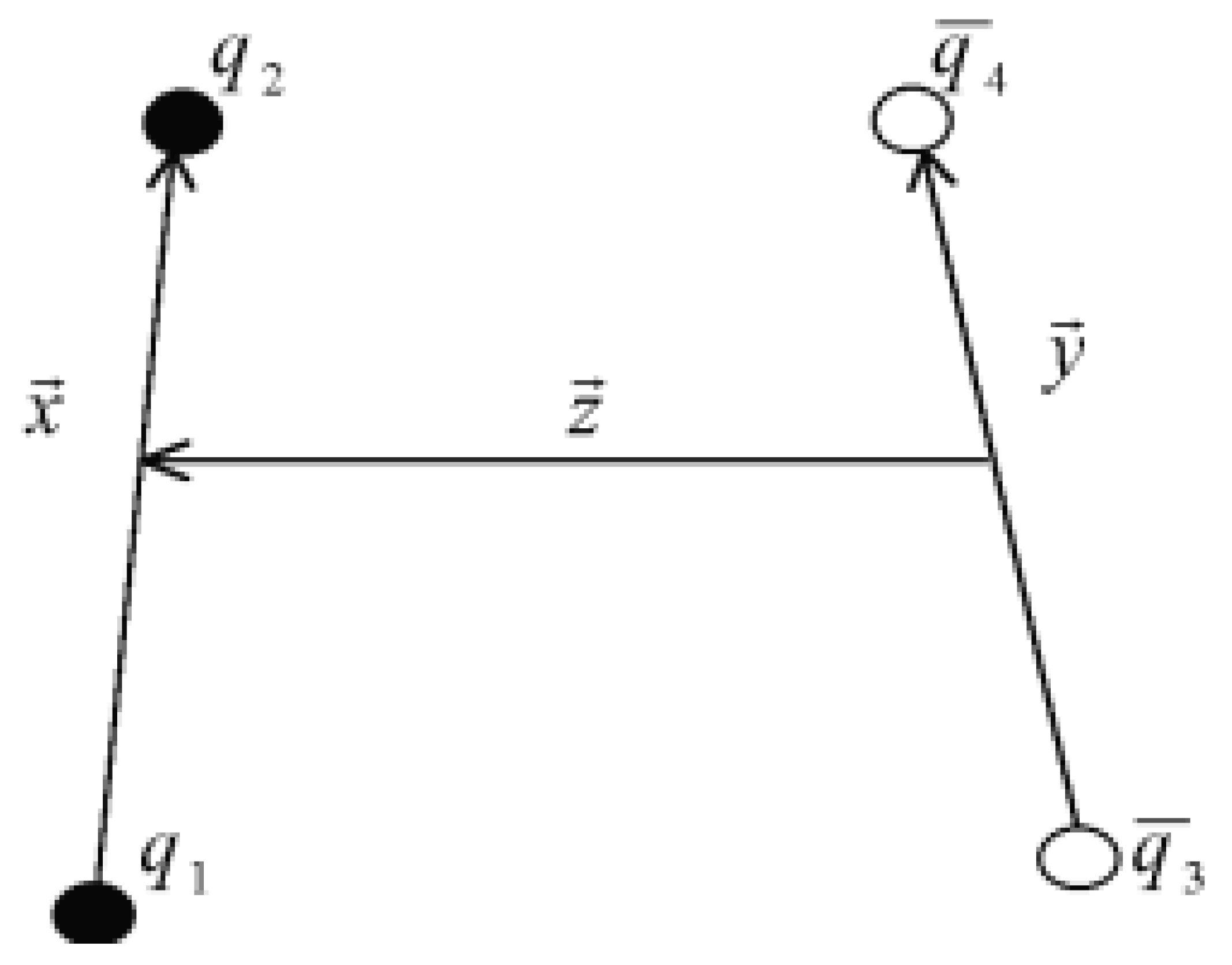
For the description of the $q_1{q}_2\overline{q_3}\overline{q_4}$ wave function we consider the four-body Jacobi coordinates depicted in Figure 2:

$$\begin{array}{lll}\overrightarrow{x}& =& {\overrightarrow{r}}_1-{\overrightarrow{r}}_2\\ \overrightarrow{y}& =& {\overrightarrow{r}}_3-{\overrightarrow{r}}_4\\ \overrightarrow{z}& =& \frac{m_1{\overrightarrow{r}}_1+m_2{\overrightarrow{r}}_2}{m_1+m_2}-\frac{m_3{\overrightarrow{r}}_3+m_4{\overrightarrow{r}}_4}{m_3+m_4}\\ \overrightarrow{R}& =& \frac{\sum m_i{\overrightarrow{r}}_i}{\sum m_i}\end{array}$$

(4)

where indices 1 and 2 will stand for quarks and 3 and 4 for antiquarks. Let us now describe each component of the variational wave function (efr) separately. The total wave function should have well-defined permutation properties under the exchange of identical particles: quarks or antiquarks. The Pauli principle must be satisfied for each subsystem of identical particles2. This imposes restrictions on the quantum numbers of the basis states.

2.3. Color space

There are three different ways of coupling two quarks and two antiquarks into a colorless state:

$$\begin{array}{lll}[(q_1{q}_2)({\overline{q}}_3{\overline{q}}_4)]& \equiv & \{|{\overline{3}}_{12}{3}_{34}\rangle ,|6_{12}{\overline{6}}_{34}\rangle \}\equiv {\{|\overline{3}3\rangle }_c^{12},|6\overline{6}{\rangle }_c^{12}\}\end{array}$$

(5a)

$$\begin{array}{lll}[(q_1{\overline{q}}_3)(q_2{\overline{q}}_4)]& \equiv & \{|1_{13}{1}_{24}\rangle ,|8_{13}{8}_{24}\rangle \}\equiv {\{|11\rangle }_c{,|88\rangle }_c\}\end{array}$$

(5b)

$$\begin{array}{lll}[(q_1{\overline{q}}_4)(q_2{\overline{q}}_3)]& \equiv & \{|1_{14}{1}_{23}\rangle ,|8_{14}{8}_{23}\rangle \}\equiv {\{|1^{\prime }{1}^{\prime }\rangle }_c,|8^{\prime }{8}^{\prime }{\rangle }_c\}\end{array}$$

(5c)

being the three of them orthonormal basis. Each coupling scheme allows to define a color basis where the four-quark problem can be solved. Only two of these states have well defined permutation properties: $|\overline{3}{3\rangle }_c^{12}$, is antisymmetric under the exchange of both quarks and antiquarks, $(AA)$, and $|6\overline{6}{\rangle }_c^{12}$ is symmetric, $(SS)$. Therefore, the basis Equation 5a is the most suitable one to deal with the Pauli principle. The other two, Equations 5b, 5c are hybrid bases containing singlet-singlet (physical) and octet-octet (hidden-color) vectors. The three basis are related through [15,16]:

$$\begin{array}{lll}{|11\rangle }_c& =& \sqrt{\frac{1}{3}}|\overline{3}{3\rangle }_c^{12}+\sqrt{\frac{2}{3}}{|6\overline{6}\rangle }_c^{12}\\ {|88\rangle }_c& =& -\sqrt{\frac{2}{3}}|\overline{3}{3\rangle }_c^{12}+\sqrt{\frac{1}{3}}{|6\overline{6}\rangle }_c^{12},\end{array}$$

(6)

and

$$\begin{array}{lll}|1^{\prime }{1}^{\prime }{\rangle }_c& =& -\sqrt{\frac{1}{3}}|\overline{3}{3\rangle }_c^{12}+\sqrt{\frac{2}{3}}{|6\overline{6}\rangle }_c^{12}\\ |8^{\prime }{8}^{\prime }{\rangle }_c& =& \sqrt{\frac{2}{3}}|\overline{3}{3\rangle }_c^{12}+\sqrt{\frac{1}{3}}{|6\overline{6}\rangle }_c^{12}\end{array}$$

(7)

To evaluate color matrix elements the two-body color operators are introduced in the same manner as in angular momentum theory,

$${\overrightarrow{\lambda }}_i·{\overrightarrow{\lambda }}_j=\frac{1}{2}\left({\overrightarrow{\lambda }}_{ij}^2-{\overrightarrow{\lambda }}_i^2-{\overrightarrow{\lambda }}_j^2\right)$$

(8)

where ${\overrightarrow{\lambda }}_i$ are the $SU{(3)}_c$ Gell-Mann matrices acting on quark i, and ${\overrightarrow{\lambda }}_{ij}^2$ is the Casimir operator. For an irreducible representation $\psi (\lambda \mu )$, the eigenvalue of the Casimir operator is given by:

$${\overrightarrow{\lambda }}_{ij}^2\psi (\lambda \mu )=\frac{4}{3}\left({\lambda }^2+{\mu }^2+\lambda \mu +3\lambda +3\mu \right)\psi (\lambda \mu )$$

(9)

In the color space a quark is described by $3_c=(10)$ and an antiquark by ${\overline{3}}_c=(01)$, so

$$\begin{array}{lll}{\overrightarrow{\lambda }}_i^2\psi (10)& =& {\overrightarrow{\lambda }}_i^2[3_c]=\frac{16}{3}[3_c]=\frac{16}{3}\psi (10)\\ {\overrightarrow{\lambda }}_i^2\psi (01)& =& {\overrightarrow{\lambda }}_i^2[{\overline{3}}_c]=\frac{16}{3}[{\overline{3}}_c]=\frac{16}{3}\psi (01)\end{array}$$

(10)

Two quarks in a symmetric state, 6 or $\overline{6}$, have $(\lambda \mu )=(20)$ and therefore

$${\overrightarrow{\lambda }}_i^2\psi (20)={\overrightarrow{\lambda }}_i^2[6_c]={\overrightarrow{\lambda }}_i^2[{\overline{6}}_c]=\frac{40}{3}\psi (20)$$

(11)

while two quarks in an antisymmetric state, 3 or $\overline{3}$, have $(\lambda \mu )=(01)$, being the same value as Equation (10). Using these expressions, the color matrix elements summarized in

Table 1. Color matrix elements.

$\widehat{\mathit{O}}$	$({\overrightarrow{\mathit{\lambda }}}_1·{\overrightarrow{\mathit{\lambda }}}_2)$	$({\overrightarrow{\mathit{\lambda }}}_3·{\overrightarrow{\mathit{\lambda }}}_4)$	$({\overrightarrow{\mathit{\lambda }}}_1·{\overrightarrow{\mathit{\lambda }}}_3)$	$({\overrightarrow{\mathit{\lambda }}}_2·{\overrightarrow{\mathit{\lambda }}}_4)$	$({\overrightarrow{\mathit{\lambda }}}_1·{\overrightarrow{\mathit{\lambda }}}_4)$	$({\overrightarrow{\mathit{\lambda }}}_2·{\overrightarrow{\mathit{\lambda }}}_3)$
${}_c^{12}\langle \overline{3}3|\widehat{O}{|\overline{3}3\rangle }_c^{12}$	$-8/3$	$-8/3$	$-4/3$	$-4/3$	$-4/3$	$-4/3$
${}_c^{12}\langle 6\overline{6}|\widehat{O}{|6\overline{6}\rangle }_c^{12}$	$4/3$	$4/3$	$-10/3$	$-10/3$	$-10/3$	$-10/3$
${}_c^{12}\langle \overline{3}3|\widehat{O}{|6\overline{6}\rangle }_c^{12}$	0	0	$-2\sqrt{2}$	$-2\sqrt{2}$	$2\sqrt{2}$	$2\sqrt{2}$

, may be easily evaluated.

2.4. Spin space

The spin part of the wave function can be written as

$${\left[{(s_1{s}_2)}_{S_{12}}{(s_3{s}_4)}_{S_{34}}\right]}_S\equiv {|S_{12}{S}_{34}\rangle }_s^{12}$$

(12)

where the spin of the two quarks (antiquarks) is coupled to $S_{12}$ ($S_{34}$). Two identical spin-$1/2$ fermions in a $S=0$ state are antisymmetric $(A)$ under permutations while those coupled to $S=1$ are symmetric $(S)$. In

Table 2. Spin basis vectors for all possible total spin states $(S)$. The “Symmetry” column stands for the symmetry properties of the pair of quarks and antiquarks.

S	Vector	Symmetry
0	${|00\rangle }_s^{12}$	AA
	${|11\rangle }_s^{12}$	SS
	${|01\rangle }_s^{12}$	AS
1	${|10\rangle }_s^{12}$	SA
	${|11\rangle }_s^{12}$	SS
2	${|11\rangle }_s^{12}$	SS

we have included the corresponding vectors for each total spin together with their symmetry properties.

Using this notation is straightforward to evaluate the four-body spin matrix elements,

$${}_s^{12}\langle S_{12}{S}_{34}|{\overrightarrow{\sigma }}_i·{\overrightarrow{\sigma }}_j{|S_{12}^{\prime }{S}_{34}^{\prime }\rangle }_s^{12}=\left[2S_{ij}(S_{ij}+1)-3\right]{\delta }_{S_{12},S_{12}^{\prime }}{\delta }_{S_{34},S_{34}^{\prime }}{\delta }_{S,S^{\prime }}$$

(13)

for $(ij)=(12)$ or (34) and where ${\overrightarrow{\sigma }}_i$ is the spin operator acting over particle i. To calculate the other spin operators we should reorder the spin wave function [14]

$$\begin{array}{c}{\left[{(s_1{s}_2)}_{S_{12}}{(s_3{s}_4)}_{S_{34}}\right]}_S=\sum _{k,l}{(-1)}^{2S_{12}+s_2+2s_3+s_4+l+S}\sqrt{2k+1}\sqrt{2l+1}\sqrt{2S_{12}+1}\sqrt{2S_{34}+1}\\ \left\{\begin{array}{ccc}{S}_{12}& s_3& k\\ s_4& S& S_{34}\end{array}\right\}\left\{\begin{array}{ccc}{s}_2& s_1& S_{12}\\ s_3& k& l\end{array}\right\}{\left[{\left[{(s_1{s}_3)}_l{s}_2\right]}_k{s}_4\right]}_S\end{array}$$

(14)

Now one can calculate the matrix element for the case $s_1=s_2=s_3=s_4=\frac{1}{2}$,

$$\begin{array}{l}{}_s^{12}\langle S_{12}{S}_{34}|{\overrightarrow{\sigma }}_1·{\overrightarrow{\sigma }}_3{|S_{12}^{\prime }{S}_{34}^{\prime }\rangle }_s^{12}=\\ =\sqrt{2S_{12}+1}\sqrt{2S_{12}^{\prime }+1}\sqrt{2S_{34}+1}\sqrt{2S_{34}^{\prime }+1}\sum _{k,l}(2k+1)(2l+1)\left[2l(l+1)-3\right]\times \\ \times \left\{\begin{array}{ccc}{S}_{12}& 1/2& k\\ 1/2& S& S_{34}\end{array}\right\}\left\{\begin{array}{ccc}{S}_{12}^{\prime }& 1/2& k\\ 1/2& S& S_{34}^{\prime }\end{array}\right\}\left\{\begin{array}{ccc}1/2& 1/2& S_{12}\\ 1/2& k& l\end{array}\right\}\left\{\begin{array}{ccc}1/2& 1/2& S_{12}^{\prime }\\ 1/2& k& l\end{array}\right\}\end{array}$$

(15)

The same can be done for the other spin operators, $({\overrightarrow{\sigma }}_1·{\overrightarrow{\sigma }}_4)$, $({\overrightarrow{\sigma }}_2·{\overrightarrow{\sigma }}_4)$ and $({\overrightarrow{\sigma }}_2·{\overrightarrow{\sigma }}_3)$, using the expressions given above. The results are resumed in

Table 3. Spin matrix elements.

S		$({\overrightarrow{\mathit{\sigma }}}_1·{\overrightarrow{\mathit{\sigma }}}_2)$	$({\overrightarrow{\mathit{\sigma }}}_3·{\overrightarrow{\mathit{\sigma }}}_4)$	$({\overrightarrow{\mathit{\sigma }}}_1·{\overrightarrow{\mathit{\sigma }}}_3)$	$({\overrightarrow{\mathit{\sigma }}}_2·{\overrightarrow{\mathit{\sigma }}}_4)$	$({\overrightarrow{\mathit{\sigma }}}_1·{\overrightarrow{\mathit{\sigma }}}_4)$	$({\overrightarrow{\mathit{\sigma }}}_2·{\overrightarrow{\mathit{\sigma }}}_3)$
	${}_s^{12}\langle 00|\widehat{O}{|00\rangle }_s^{12}$	$-3$	$-3$	0	0	0	0
0	${}_s^{12}\langle 11|\widehat{O}{|11\rangle }_s^{12}$	1	1	$-2$	$-2$	$-2$	$-2$
	${}_s^{12}\langle 00|\widehat{O}{|11\rangle }_s^{12}$	0	0	$-\sqrt{3}$	$-\sqrt{3}$	$\sqrt{3}$	$\sqrt{3}$
	${}_s^{12}\langle 01|\widehat{O}{|01\rangle }_s^{12}$	$-3$	1	0	0	0	0
	${}_s^{12}\langle 10|\widehat{O}{|10\rangle }_s^{12}$	1	$-3$	0	0	0	0
1	${}_s^{12}\langle 11|\widehat{O}{|11\rangle }_s^{12}$	1	1	$-1$	$-1$	$-1$	$-1$
	${}_s^{12}\langle 01|\widehat{O}{|10\rangle }_s^{12}$	0	0	1	1	$-1$	$-1$
	${}_s^{12}\langle 10|\widehat{O}{|11\rangle }_s^{12}$	0	0	$\sqrt{2}$	$-\sqrt{2}$	$-\sqrt{2}$	$\sqrt{2}$
	${}_s^{12}\langle 01|\widehat{O}{|11\rangle }_s^{12}$	0	0	$-\sqrt{2}$	$\sqrt{2}$	$-\sqrt{2}$	$\sqrt{2}$
2	${}_s^{12}\langle 11|\widehat{O}{|11\rangle }_s^{12}$	1	1	1	1	1	1

.

2.5. Flavor space

Before discussing the flavor part of the wave function one must specify the required flavor symmetry, $SU(2)$ or $SU(3)$. In the former case, u and d quarks are identical whether in the latter, u, d, and s are indistinguishable. In the following, n will stand for light u and d quarks and Q for heavy ones, c or b. s quarks will be considered heavy if flavor $SU(2)$ is assumed and light otherwise.

For the flavor part one finds several different possible four-quark states depending on the number of light quarks. They can be classified depending on whether they are made of undistinguishable quarks in one of the pairs (and therefore the Pauli principle must be imposed) or not. In following subsections we will discuss the important role played by the Pauli principle in the description of the four-quark states properties. This classification is illustrated in

Table 4. Pauli-based classification of four-quark states. ✓ indicates that the quark/antiquark pair requires the application of the Pauli principle, being the notation (pair of quarks, pair of antiquarks). The third and fourth columns contain the recoupling corresponding to bases 5b and 5c.

(12)(34)	Pauli	(13)(24)	(14)(23)
$(nn)(\overline{n}\overline{n})$	$(✓,✓)$	$(n\overline{n})(n\overline{n})$	$(n\overline{n})(n\overline{n})$
$(nn)(\overline{n}\overline{Q})$	$(✓,X)$	$(n\overline{n})(n\overline{Q})$	$(n\overline{Q})(n\overline{n})$
$(nn)({\overline{Q}}_1{\overline{Q}}_2)$	$(✓,✓$ if ${\overline{Q}}_1={\overline{Q}}_2$)	$(n{\overline{Q}}_1)(n{\overline{Q}}_2)$	$(n{\overline{Q}}_2)(n{\overline{Q}}_1)$
$(n{Q}_1)(\overline{n}{\overline{Q}}_2)$	$(X,X$)	$(n\overline{n})(Q_1{\overline{Q}}_2)$	$(n{\overline{Q}}_2)(Q_1\overline{n})$
$(n{Q}_1)({\overline{Q}}_2{\overline{Q}}_3)$	$(X,✓$ if ${\overline{Q}}_2={\overline{Q}}_3$)	$(n{\overline{Q}}_2)(Q_1{\overline{Q}}_3)$	$(n{\overline{Q}}_3)(Q_1{\overline{Q}}_2)$
$(Q_1{Q}_2)({\overline{Q}}_3{\overline{Q}}_4)$	(✓ if $Q_1=Q_2$, ✓ if ${\overline{Q}}_3={\overline{Q}}_4$)	$(Q_1{\overline{Q}}_3)(Q_2{\overline{Q}}_4)$	$(Q_1{\overline{Q}}_4)(Q_2{\overline{Q}}_3)$

. Symmetry properties of the flavor wave function are summarized in

Table 5. Symmetry properties of the flavor wave function under the exchange of quarks (the same holds for antiquarks). ${}^{†}$ If flavor $SU(3)$ is assumed, symmetric and antisymmetric flavor wave functions with $I=1/2$ can be constructed, i.e., $(us\pm su)/\sqrt{2}$).

Flavor	Symmetry
$nn$$I=0$	A
$nn$$I=1$	S
$nn$$I=1/2^{†}$	S/A
$QQ$$I=0$	S

.

The flavor $SU(2)$ matrix elements can be evaluated by means of the same relations shown in Section 2.4. For those corresponding to flavor $SU(3)$ the procedure will require the explicit construction of the flavor wave function by means of the $SU(3)$ isoscalar factors given in [15,16]3. As an example we evaluate some of the flavor matrix elements needed for the description of heavy-light tetraquarks. They can be obtained using the matrix expression of ${\lambda }^a$,

$$\begin{array}{lll}{\lambda }^1=\left(\begin{array}{ccc}0& 1& 0\\ 1& 0& 0\\ 0& 0& 0\end{array}\right)& {\lambda }^2=\left(\begin{array}{ccc}0& -i& 0\\ i& 0& 0\\ 0& 0& 0\end{array}\right)& {\lambda }^3=\left(\begin{array}{ccc}1& 0& 0\\ 0& -1& 0\\ 0& 0& 0\end{array}\right)\\ {\lambda }^4=\left(\begin{array}{ccc}0& 0& 1\\ 0& 0& 0\\ 1& 0& 0\end{array}\right)& {\lambda }^5=\left(\begin{array}{ccc}0& 0& -i\\ 0& 0& 0\\ i& 0& 0\end{array}\right)& {\lambda }^6=\left(\begin{array}{ccc}0& 0& 0\\ 0& 0& 1\\ 0& 1& 0\end{array}\right)\\ {\lambda }^7=\left(\begin{array}{ccc}0& 0& 0\\ 0& 0& -i\\ 0& i& 0\end{array}\right)& {\lambda }^8=\left(\begin{array}{ccc}\frac{1}{\sqrt{3}}& 0& 0\\ 0& \frac{1}{\sqrt{3}}& 0\\ 0& 0& \frac{-2}{\sqrt{3}}\end{array}\right)& \end{array}$$

(16)

where, following the same convention, quarks and antiquarks are given by,

$$\begin{array}{ll}u& =\overline{u}=(1,0,0)\\ d& =\overline{d}=(0,1,0)\\ s& =\overline{s}=(0,0,1)\end{array}$$

(17)

The tetraquark flavor wave function corresponding to two light quarks coupled to total isospin I with $I_z=0$ and two heavy antiquarks can be written as

$$\left|\psi \right.〉=\frac{1}{\sqrt{2}}[ud+{(-1)}^{I+1}du][\overline{s}\overline{s}]$$

(18)

A typical flavor operator is

$${\overrightarrow{\tau }}_i·{\overrightarrow{\tau }}_j=\sum _{a=1}^3{\lambda }_i^a{\lambda }_j^a$$

(19)

where ${\lambda }_i^a$ are the $SU(3)$ flavor matrices defined above and ${\tau }_i$ are the isospin Pauli matrices, both acting on quark i. So the same expression obtained for the spin operators holds here:

$$〈\psi \left|\sum _{a=1}^3{\lambda }_1^a{\lambda }_2^a\right|\psi 〉=\left\{\begin{array}{cc}I=0& \to -3\\ I=1& \to 1\end{array}\right.$$

(20)

Alternatively one can write the flavor matrix element as

$$\begin{array}{lll}〈\psi |\sum _{a=1}^3{\lambda }_1^a{\lambda }_2^a|\psi 〉& =& 〈\frac{ud+{(-1)}^{I+1}du}{\sqrt{2}}\left|\sum _{a=1}^3{\lambda }_1^a{\lambda }_2^a\right|\frac{ud+{(-1)}^{I+1}du}{\sqrt{2}}〉=\\ & =& \frac{1}{2}\sum _{a=1}^3\{〈ud\left|{\lambda }_1^a{\lambda }_2^a\right|ud〉+〈du\left|{\lambda }_1^a{\lambda }_2^a\right|du〉+\\ & +& {(-1)}^{I+1}〈du\left|{\lambda }_1^a{\lambda }_2^a\right|ud〉+{(-1)}^{I+1}〈ud\left|{\lambda }_1^a{\lambda }_2^a\right|du〉\}=\\ & =& \sum _{a=1}^3\left\{〈u|{\lambda }^a|u〉〈d|{\lambda }^a|d〉+{(-1)}^{I+1}{\left|〈u|{\lambda }^a|d〉\right|}^2\right\}=\\ & =& -1+2{(-1)}^{I+1}=\left\{\begin{array}{cc}I=0& -3\\ I=1& 1\end{array}\right.\end{array}$$

(21)

Other matrix elements of interest are,

$$\begin{array}{l}〈\psi |{\lambda }_1^8{\lambda }_2^8|\psi 〉=\frac{1}{3}\\ 〈\psi |{\lambda }_3^8{\lambda }_4^8|\psi 〉=\frac{4}{3}\\ 〈\psi |{\lambda }_1^8{\lambda }_3^8|\psi 〉=〈\psi |{\lambda }_2^8{\lambda }_3^8|\psi 〉=〈\psi |{\lambda }_1^8{\lambda }_4^8|\psi 〉=〈\psi |{\lambda }_2^8{\lambda }_4^8|\psi 〉=-\frac{2}{3}\end{array}$$

(22)

2.6. Radial space

The most general radial wave function with orbital angular momentum $L=0$ may depend on the six scalar quantities that can be constructed with the Jacobi coordinates of the system, they are: ${\overrightarrow{x}}^2$, ${\overrightarrow{y}}^2$, ${\overrightarrow{z}}^2$, $\overrightarrow{x}·\overrightarrow{y}$, $\overrightarrow{x}·\overrightarrow{z}$ and $\overrightarrow{y}·\overrightarrow{z}$. We define the variational spatial wave function as a linear combination of generalized Gaussians,

$$\left|R_{s_4}\right.〉=\sum _{i=1}^n{\beta }_{s_4}^{(i)}{R}_{s_4}^i(\overrightarrow{x},\overrightarrow{y},\overrightarrow{z})=\sum _{i=1}^n{\beta }_{s_4}^{(i)}{R}_{s_4}^i$$

(23)

where n is the number of Gaussians we use for each color-spin-flavor component. $R_{s_4}^i$ depends on six variational parameters, $a_s^i$, $b_s^i$, $c_s^i$, $d_s^i$, $e_s^i$, and $f_s^i$, one for each scalar quantity. Therefore, any tetraquark will depend on $6\times n\times n_s$ variational parameters (where $n_s$ is the number of different channels allowed by the Pauli Principle). Equation (23) should have well defined permutation symmetry under the exchange of both quarks and antiquarks,

$$\begin{array}{lll}{P}_{12}(\overrightarrow{x}\to -\overrightarrow{x})R_{s_4}^i& =& P_x{R}_{s_4}^i\\ P_{34}(\overrightarrow{y}\to -\overrightarrow{y})R_{s_4}^i& =& P_y{R}_{s_4}^i\end{array}$$

(24)

where $P_x$ and $P_y$ are $-1$ for antisymmetric states, $(A)$, and $+1$ for symmetric ones, $(S)$. One can build the following radial combinations, $(P_x{P}_y)=(SS)$, $(SA)$, $(AS)$ and $(AA)$:

$$\begin{array}{lll}(SS)\Rightarrow R_1^i& =& \mathrm{Exp}\left(-a_s^i{\overrightarrow{x}}^2-b_s^i{\overrightarrow{y}}^2-c_s^i{\overrightarrow{z}}^2-d_s^i\overrightarrow{x}\overrightarrow{y}-e_s^i\overrightarrow{x}\overrightarrow{z}-f_s^i\overrightarrow{y}\overrightarrow{z}\right)\\ & +& \mathrm{Exp}\left(-a_s^i{\overrightarrow{x}}^2-b_s^i{\overrightarrow{y}}^2-c_s^i{\overrightarrow{z}}^2+d_s^i\overrightarrow{x}\overrightarrow{y}+e_s^i\overrightarrow{x}\overrightarrow{z}-f_s^i\overrightarrow{y}\overrightarrow{z}\right)\\ & +& \mathrm{Exp}\left(-a_s^i{\overrightarrow{x}}^2-b_s^i{\overrightarrow{y}}^2-c_s^i{\overrightarrow{z}}^2-d_s^i\overrightarrow{x}\overrightarrow{y}+e_s^i\overrightarrow{x}\overrightarrow{z}+f_s^i\overrightarrow{y}\overrightarrow{z}\right)\end{array}$$

(25)

$$\begin{array}{lll}(SA)\Rightarrow R_2^i& =& \mathrm{Exp}\left(-a_s^i{\overrightarrow{x}}^2-b_s^i{\overrightarrow{y}}^2-c_s^i{\overrightarrow{z}}^2-d_s^i\overrightarrow{x}\overrightarrow{y}-e_s^i\overrightarrow{x}\overrightarrow{z}-f_s^i\overrightarrow{y}\overrightarrow{z}\right)\\ & -& \mathrm{Exp}\left(-a_s^i{\overrightarrow{x}}^2-b_s^i{\overrightarrow{y}}^2-c_s^i{\overrightarrow{z}}^2+d_s^i\overrightarrow{x}\overrightarrow{y}-e_s^i\overrightarrow{x}\overrightarrow{z}+f_s^i\overrightarrow{y}\overrightarrow{z}\right)\\ & +& \mathrm{Exp}\left(-a_s^i{\overrightarrow{x}}^2-b_s^i{\overrightarrow{y}}^2-c_s^i{\overrightarrow{z}}^2+d_s^i\overrightarrow{x}\overrightarrow{y}+e_s^i\overrightarrow{x}\overrightarrow{z}-f_s^i\overrightarrow{y}\overrightarrow{z}\right)\\ & -& \mathrm{Exp}\left(-a_s^i{\overrightarrow{x}}^2-b_s^i{\overrightarrow{y}}^2-c_s^i{\overrightarrow{z}}^2-d_s^i\overrightarrow{x}\overrightarrow{y}+e_s^i\overrightarrow{x}\overrightarrow{z}+f_s^i\overrightarrow{y}\overrightarrow{z}\right)\end{array}$$

(26)

$$\begin{array}{lll}(AS)\Rightarrow R_3^i& =& \mathrm{Exp}\left(-a_s^i{\overrightarrow{x}}^2-b_s^i{\overrightarrow{y}}^2-c_s^i{\overrightarrow{z}}^2-d_s^i\overrightarrow{x}\overrightarrow{y}-e_s^i\overrightarrow{x}\overrightarrow{z}-f_s^i\overrightarrow{y}\overrightarrow{z}\right)\\ & +& \mathrm{Exp}\left(-a_s^i{\overrightarrow{x}}^2-b_s^i{\overrightarrow{y}}^2-c_s^i{\overrightarrow{z}}^2+d_s^i\overrightarrow{x}\overrightarrow{y}-e_s^i\overrightarrow{x}\overrightarrow{z}+f_s^i\overrightarrow{y}\overrightarrow{z}\right)\\ & -& \mathrm{Exp}\left(-a_s^i{\overrightarrow{x}}^2-b_s^i{\overrightarrow{y}}^2-c_s^i{\overrightarrow{z}}^2+d_s^i\overrightarrow{x}\overrightarrow{y}+e_s^i\overrightarrow{x}\overrightarrow{z}-f_s^i\overrightarrow{y}\overrightarrow{z}\right)\\ & -& \mathrm{Exp}\left(-a_s^i{\overrightarrow{x}}^2-b_s^i{\overrightarrow{y}}^2-c_s^i{\overrightarrow{z}}^2-d_s^i\overrightarrow{x}\overrightarrow{y}+e_s^i\overrightarrow{x}\overrightarrow{z}+f_s^i\overrightarrow{y}\overrightarrow{z}\right)\end{array}$$

(27)

$$\begin{array}{lll}(AA)\Rightarrow R_4^i& =& \mathrm{Exp}\left(-a_s^i{\overrightarrow{x}}^2-b_s^i{\overrightarrow{y}}^2-c_s^i{\overrightarrow{z}}^2-d_s^i\overrightarrow{x}\overrightarrow{y}-e_s^i\overrightarrow{x}\overrightarrow{z}-f_s^i\overrightarrow{y}\overrightarrow{z}\right)\\ & -& \mathrm{Exp}\left(-a_s^i{\overrightarrow{x}}^2-b_s^i{\overrightarrow{y}}^2-c_s^i{\overrightarrow{z}}^2+d_s^i\overrightarrow{x}\overrightarrow{y}-e_s^i\overrightarrow{x}\overrightarrow{z}+f_s^i\overrightarrow{y}\overrightarrow{z}\right)\\ & -& \mathrm{Exp}\left(-a_s^i{\overrightarrow{x}}^2-b_s^i{\overrightarrow{y}}^2-c_s^i{\overrightarrow{z}}^2+d_s^i\overrightarrow{x}\overrightarrow{y}+e_s^i\overrightarrow{x}\overrightarrow{z}-f_s^i\overrightarrow{y}\overrightarrow{z}\right)\\ & +& \mathrm{Exp}\left(-a_s^i{\overrightarrow{x}}^2-b_s^i{\overrightarrow{y}}^2-c_s^i{\overrightarrow{z}}^2-d_s^i\overrightarrow{x}\overrightarrow{y}+e_s^i\overrightarrow{x}\overrightarrow{z}+f_s^i\overrightarrow{y}\overrightarrow{z}\right)\end{array}$$

(28)

By defiing the function

$$g(s_1,s_2,s_3)=\mathrm{Exp}\left(-a_s^i{\overrightarrow{x}}^2-b_s^i{\overrightarrow{y}}^2-c_s^i{\overrightarrow{z}}^2-s_1{d}_s^i\overrightarrow{x}\overrightarrow{y}-s_2{e}_s^i\overrightarrow{x}\overrightarrow{z}-s_3{f}_s^i\overrightarrow{y}\overrightarrow{z}\right)$$

(29)

we can build the vectors

$$\overrightarrow{G_s^i}=\left(\begin{array}{c}g(+,+,+)\\ g(-,+,-)\\ g(-,-,+)\\ g(+,-,-)\end{array}\right)$$

(30)

and

$$\begin{array}{lll}\overrightarrow{{\alpha }_{SS}}& =& (+,+,+,+)\\ \overrightarrow{{\alpha }_{SA}}& =& (+,-,+,-)\\ \overrightarrow{{\alpha }_{AS}}& =& (+,+,-,-)\\ \overrightarrow{{\alpha }_{AA}}& =& (+,-,-,+)\end{array}$$

(31)

what allows to write in a compact way Equations 25–28,

$$\begin{array}{lll}(SS)& \Rightarrow & R_1^i=\overrightarrow{{\alpha }_{SS}}·\overrightarrow{G_s^i}\\ (SA)& \Rightarrow & R_2^i=\overrightarrow{{\alpha }_{SA}}·\overrightarrow{G_s^i}\\ (AS)& \Rightarrow & R_3^i=\overrightarrow{{\alpha }_{AS}}·\overrightarrow{G_s^i}\\ (AA)& \Rightarrow & R_4^i=\overrightarrow{{\alpha }_{AA}}·\overrightarrow{G_s^i}\end{array}$$

(32)

Such a radial wave function includes all possible relative orbital angular momenta coupled to $L=0$. This can be seen through the relation:

$$\begin{array}{l}\mathrm{Exp}\left(-d_s^i\overrightarrow{x}\overrightarrow{y}-e_s^i\overrightarrow{x}\overrightarrow{z}-f_s^i\overrightarrow{y}\overrightarrow{z}\right)=\frac{1}{\sqrt{4\pi }}\sum _{{\ell }_x=0}^{\infty }\sum _{{\ell }_y=0}^{\infty }\sum _{{\ell }_z=0}^{\infty }{\left[{[Y_{{\ell }_x}(\widehat{x})Y_{{\ell }_y}(\widehat{y})]}_{{\ell }_z}{Y}_{{\ell }_z}(\widehat{z})\right]}_0\\ \sum _{{\ell }_1,{\ell }_2,{\ell }_3}(2{\ell }_1+1)(2{\ell }_2+1)(2{\ell }_3+1)〈{\ell }_{1}0{\ell }_{2}0|{\ell }_x〉〈{\ell }_{1}0{\ell }_{3}0|{\ell }_y〉〈{\ell }_{2}0{\ell }_{3}0|{\ell }_z〉\left\{\begin{array}{ccc}{\ell }_x& {\ell }_y& {\ell }_z\\ {\ell }_3& {\ell }_2& {\ell }_1\end{array}\right\}\\ \left(\sqrt{\frac{\pi }{2d_s^{i}xy}}{I}_{{\ell }_1+1/2}(d_s^{i}xy)\right)\left(\sqrt{\frac{\pi }{2e_s^{i}xz}}{I}_{{\ell }_2+1/2}(e_s^{i}xz)\right)\left(\sqrt{\frac{\pi }{2f_s^{i}yz}}{I}_{{\ell }_3+1/2}(f_s^{i}yz)\right)\end{array}$$

(33)

where ${\ell }_x$, ${\ell }_y$ and ${\ell }_z$ are the orbital angular momenta associated to coordinates $\overrightarrow{x}$, $\overrightarrow{y}$ and $\overrightarrow{z}$, and $I_a(x)$ are the modified Bessel functions.

The radial wave functions defined above have also well-defined symmetry properties on the $\overrightarrow{z}$ coordinate. Being $P_{(12)(34)}(\overrightarrow{z}\to -\overrightarrow{z})R_{s_4}^i=P_z{R}_{s_4}^i$ one obtains,

$$\begin{array}{lll}{P}_{(12)(34)}{R}_1^i& =& +R_1^i\\ P_{(12)(34)}{R}_2^i& =& -R_2^i\\ P_{(12)(34)}{R}_3^i& =& -R_3^i\\ P_{(12)(34)}{R}_4^i& =& +R_4^i\end{array}$$

(34)

To evaluate radial matrix elements we will use the notation introduced in Equation 32:

$$〈R_{\gamma }^i\left|f(x,y,z)\right|R_{\beta }^j〉={\int }_V({\overrightarrow{\alpha }}_{S_{\gamma }}·{\overrightarrow{G}}_s^i)f(x,y,z)({\overrightarrow{\alpha }}_{S_{\beta }}·{\overrightarrow{G}}_{s^{\prime }}^j)dV={\overrightarrow{\alpha }}_{S_{\gamma }}·F^{ij}·{\overrightarrow{\alpha }}_{S_{\beta }}$$

(35)

where $\gamma$ and $\beta$ stand for the symmetry of the radial wave function and $F^{ij}$ is a matrix whose element $(a,b)$ is defined through,

$$F_{ab}^{ij}={\int }_V{({\overrightarrow{G}}_s^i)}_a{({\overrightarrow{G}}_{s^{\prime }}^j)}_{b}f(x,y,z)dV$$

(36)

being ${({\overrightarrow{G}}_s^i)}_a$ the component a of the vector ${\overrightarrow{G}}_s^i$. From Equation 29 one obtains,

$$g(s_1,s_2,s_3)g(s_1^{\prime },s_2^{\prime },s_3^{\prime })=\mathrm{Exp}\left(-a_{ij}{\overrightarrow{x}}^2-b_{ij}{\overrightarrow{y}}^2-c_{ij}{\overrightarrow{z}}^2-{\overline{s}}_{ij}\overrightarrow{x}\overrightarrow{y}-{\overline{e}}_{ij}\overrightarrow{x}\overrightarrow{z}-{\overline{f}}_{ij}\overrightarrow{y}\overrightarrow{z}\right)$$

(37)

where we have shortened the previous notation according to $a_s^i\to a_i$, $a_{ij}=a_i+a_j$ and ${\overline{d}}_{ij}=(s_1{d}_i+s_1^{\prime }{d}_j)$. Therefore, all four-body radial matrix elements will contain integrals of the form

$$I={\int }_V\mathrm{Exp}\left(-a_{ij}{\overrightarrow{x}}^2-b_{ij}{\overrightarrow{y}}^2-c_{ij}{\overrightarrow{z}}^2-{\overline{s}}_{ij}\overrightarrow{x}\overrightarrow{y}-{\overline{e}}_{ij}\overrightarrow{x}\overrightarrow{z}-{\overline{f}}_{ij}\overrightarrow{y}\overrightarrow{z}\right)f(x,y,z)d\overrightarrow{x}d\overrightarrow{y}d\overrightarrow{z}$$

(38)

where the functions $f(x,y,z)$ are the potentials. Being all of them radial functions (not depending on angular variables) one can solve the previous integral by noting:

$$\int \mathrm{Exp}[-\sum _{i,j=1}^n{A}_{ij}{\overrightarrow{x}}_i{\overrightarrow{x}}_j]f\left(|\sum {\alpha }_k{\overrightarrow{x}}_k|\right)d{\overrightarrow{x}}_1...d{\overrightarrow{x}}_n={\left(\frac{{\pi }^n}{detA}\right)}^{\frac{3}{2}}4\pi {\left(\frac{{\Omega }_{ij}}{\pi }\right)}^{\frac{3}{2}}F({\Omega }_{ij},f)$$

(39)

where

$$\begin{array}{ccc}\hfill \frac{1}{{\Omega }_{ij}}& =& \overline{\alpha }·A^{-1}·\alpha \hfill \\ \hfill F(A,f)& =& \int e^{-A{u}^2}f(u)u^{2}du\hfill \\ \hfill detA& >& 0\hfill \\ \hfill \frac{1}{{\Omega }_{ij}}& >& 0\hfill \end{array}$$

(40)

One can extract some useful relations for the radial matrix elements using simple symmetry properties. Let us rewrite Equation 35

$$\begin{array}{lll}〈R_{\gamma }^i\left|f(x,y,z)\right|R_{\beta }^j〉& =& 〈R_{P_x{P}_y{P}_z}^i\left|f(x,y,z)\right|R_{P_x^{\prime }{P}_y^{\prime }{P}_z^{\prime }}^j〉\\ & =& {\int }_x{\int }_y{\int }_z{R}_{P_x{P}_y{P}_z}^{i}f(x,y,z)R_{P_x^{\prime }{P}_y^{\prime }{P}_z^{\prime }}^{j}d\overrightarrow{x}d\overrightarrow{y}d\overrightarrow{z}\end{array}$$

(41)

If $f(x,y,x)$ depends only in one coordinate, for example $\overrightarrow{x}$, the integrals over the other coordinates will be zero if one of them has different symmetry properties, $P_y\ne P_y^{\prime }$ or $P_z\ne P_z^{\prime }$ in our example. Therefore

$$\begin{array}{ccc}\hfill 〈R_{\gamma }^i\left|f(x)\right|R_{\beta }^j〉& \propto & {\delta }_{\gamma \beta }\\ \hfill 〈R_{\gamma }^i\left|f(y)\right|R_{\beta }^j〉& \propto & {\delta }_{\gamma \beta }\\ \hfill 〈R_{\gamma }^i\left|f(z)\right|R_{\beta }^j〉& \propto & {\delta }_{\gamma \beta }\\ \hfill 〈R_{\gamma }^i\left|\mathrm{Constant}\right|R_{\beta }^j〉& \propto & {\delta }_{\gamma \beta }\end{array}$$

(42)

The radial wave function described in this section is adequate to describe not only bound states, but also it is flexible enough to describe states of the two-meson continuum within a reasonable accuracy. We will came back to this point in Sect. 5.

2.7. Parity and $C-$parity

The parity of a tetraquark can be calculated as

$$P\left[R_{s_4}^i(\overrightarrow{x},\overrightarrow{y},\overrightarrow{z})\right]=R_{s_4}^i\left(\begin{array}{c}\overrightarrow{x}\to -\overrightarrow{x}\\ \overrightarrow{y}\to -\overrightarrow{y}\\ \overrightarrow{z}\to -\overrightarrow{z}\end{array}\right)={(-1)}^{{\ell }_x+{\ell }_y+{\ell }_z}{R}_{s_4}^i(\overrightarrow{x},\overrightarrow{y},\overrightarrow{z})$$

(43)

or using Equations 24 and 34,

$$P\left[R_{s_4}^i(\overrightarrow{x},\overrightarrow{y},\overrightarrow{z})\right]=P_{12}{P}_{34}{P}_{(12)(34)}{R}_{s_4}^i(\overrightarrow{x},\overrightarrow{y},\overrightarrow{z})=P_x{P}_y{P}_z{R}_{s_4}^i(\overrightarrow{x},\overrightarrow{y},\overrightarrow{z})$$

(44)

what in our case implies

$$P\left[R_{s_4}^i(\overrightarrow{x},\overrightarrow{y},\overrightarrow{z})\right]=\left\{\begin{array}{c}(+)(+)(+)R_1^i\\ (+)(-)(-)R_2^i\\ (-)(+)(-)R_3^i\\ (-)(-)(+)R_4^i\end{array}\right\}=\left\{\begin{array}{c}+R_1^i\\ +R_2^i\\ +R_3^i\\ +R_4^i\end{array}\right\}=+R_{s_4}^i(\overrightarrow{x},\overrightarrow{y},\overrightarrow{z})$$

(45)

Hence, this formalism describes positive parity states, being thus adequate to study tetraquark ground states.

From Equation 45 one can see that, not only the total wave function will be an eigenstate of the parity operator, but also each component will be. This is not the case for C-parity, where only the total wave function will be an eigenstate and therefore it must be obtained numerically for each state. The tetraquark $C-$parity will depend on the variational parameters and on the ${\beta }_s^{(i)}$ coefficients. This dependence is contained in the action of the $C-$parity operator over the different parts of the wave function which will give us the following relations:

$$C\left|R_{s_4}^i(\overrightarrow{x},\overrightarrow{y},\overrightarrow{z})\right.〉=R_{s_4}^i(\overrightarrow{y},\overrightarrow{x},-\overrightarrow{z})$$

(46)

and if $a_s^i=b_s^i$ and $e_s^i=f_s^i$ (what is a very common result),

$$C\left|R_{s_4}^i(\overrightarrow{x},\overrightarrow{y},\overrightarrow{z})\right.〉=\left\{\begin{array}{cc}{s}_4=1& \to +R_1^i\\ s_4=2& \to -R_3^i\\ s_4=3& \to -R_2^i\\ s_4=4& \to +R_4^i\end{array}\right.$$

(47)

The action of C over the spin part or the wave function is summarized in

Table 6. The action of C over the spin part or the wave function.

$\mathit{S}=0$	${\mathit{C}|00\rangle }_{\mathit{s}}^{12}=+{|00\rangle }_{\mathit{s}}^{12}$
	${C|11\rangle }_s^{12}=+{|11\rangle }_s^{12}$
	${C|01\rangle }_s^{12}=-{|10\rangle }_s^{12}$
$S=1$	${C|10\rangle }_s^{12}=-{|01\rangle }_s^{12}$
	${C|11\rangle }_s^{12}=+{|11\rangle }_s^{12}$
$S=2$	${C|11\rangle }_s^{12}=+{|11\rangle }_s^{12}$

. The action of C over the flavor part of the wave function has to be evaluated individually once the wave functions have been constructed.

2.8. $q\overline{q}\leftrightarrow qq\overline{q}\overline{q}$ mixing

Many of the possible four-quark systems may present $J^{PC}$ quantum numbers that can be reached not only by means of $qq\overline{q}\overline{q}$ configurations but also by $q\overline{q}$ ones and with similar energies. In these cases the possibility of a mixing between them cannot be discarded a priori and therefore, their most general wave function will read

$$\left|\mathrm{B}=0\right.〉=\sum _n{\Omega }_n\left|{(q\overline{q})}^n\right.〉={\Omega }_1\left|q\overline{q}\right.〉+{\Omega }_2\left|q\overline{q}q\overline{q}\right.〉+....$$

(48)

These particular systems may be described by a hamiltonian

$$H=H_0+H_1\mathrm{being}{H}_0=\left(\begin{array}{cc}{H}_{q\overline{q}}& 0\\ 0& H_{qq\overline{q}\overline{q}}\end{array}\right)H_1=\left(\begin{array}{cc}0& V_{q\overline{q}\leftrightarrow qq\overline{q}\overline{q}}\\ V_{q\overline{q}\leftrightarrow qq\overline{q}\overline{q}}& 0\end{array}\right)$$

(49)

where the nondiagonal terms can be treated perturbatively, therefore allowing to solve the two- and four-body sectors separately.

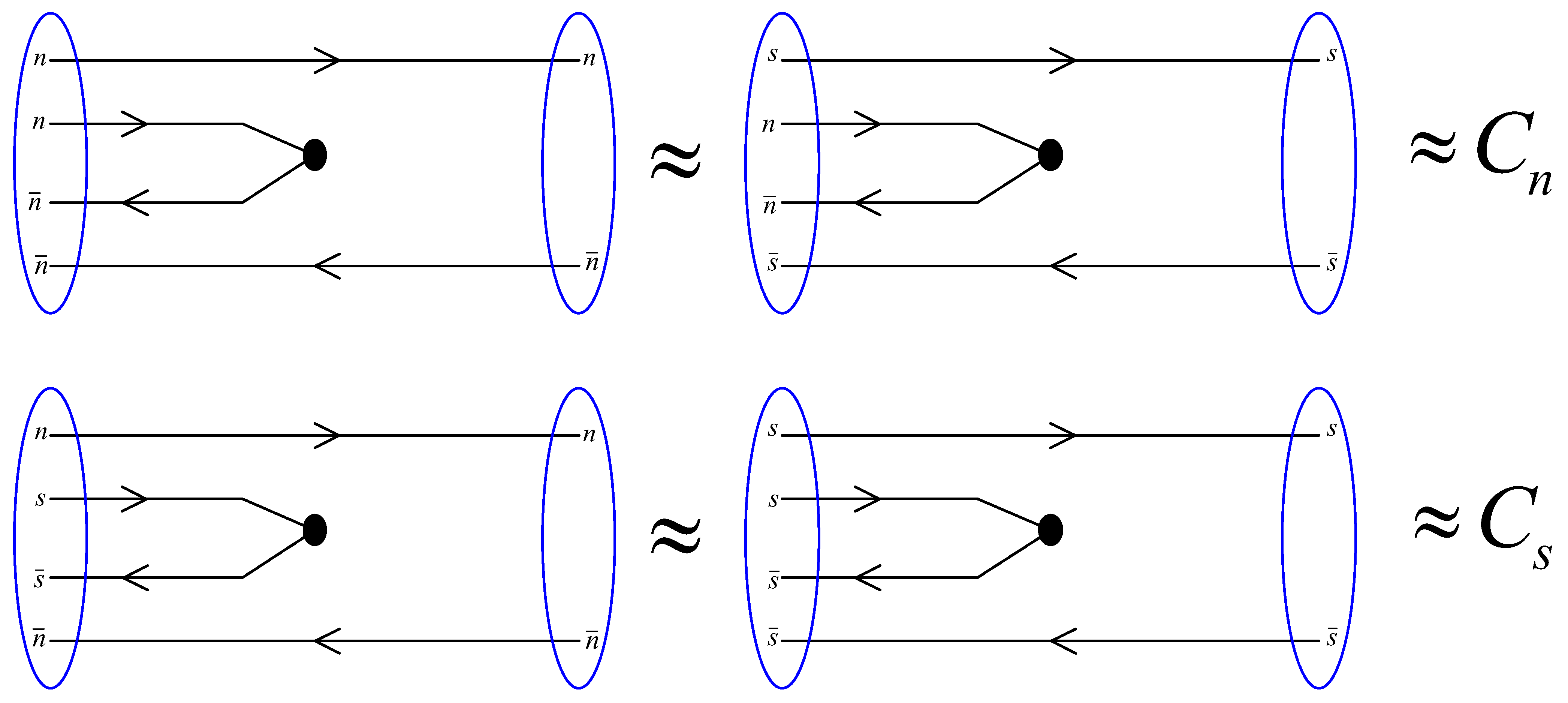
The Hamiltonian $H_1$ describes the mixing between two- and four-body configurations. Its explicit expression would require the knowledge of the operator annihilating a quark-antiquark pair into the vacuum. This could be done, for example, using a ${}^3{P}_0$ model, but the result will introduce an additional degree of uncertainty on the parametrization used to describe the vertex. Such a parametrization is determined by the energy scale at which the transition $qq\overline{q}\overline{q}\leftrightarrow q\overline{q}$ takes place. For the sake of simplicity this can be parametrized by looking to the quark pair that it is annihilated, and not to the spectator quarks that will form the final $q\overline{q}$ state:

$$V_{q\overline{q}\leftrightarrow qq\overline{q}\overline{q}}\Rightarrow \left\{\begin{array}{c}〈nn\overline{n}\overline{n}\left|V\right|n\overline{n}〉=〈ns\overline{n}\overline{s}\left|V\right|s\overline{s}〉=〈nn\overline{n}\overline{s}\left|V\right|n\overline{s}〉=C_n\\ 〈ss\overline{s}\overline{s}\left|V\right|s\overline{s}〉=〈ns\overline{n}\overline{s}\left|V\right|n\overline{n}〉=〈ns\overline{s}\overline{s}\left|V\right|n\overline{s}〉=C_s\end{array}\right.$$

(50)

A sketch of these mixing interactions is drawn in Figure 3. Such approach has been used in a series of papers to describe the light-scalar mesons and the open-charm and open-bottom meson sectors [17,18,19,20].

3. Four-Quark Stability and Threshold Determination

The color degree of freedom makes an important difference between four-quark systems and ordinary baryons or mesons. For baryons and mesons it is not possible to construct a color singlet using a subset of the constituents, thus only $q\overline{q}$ or $qqq$ states are proper solutions of the two- or three-quark interacting hamiltonian and therefore, all solutions correspond to bound states. However, this is not the case for four-quark systems. The color rearrangement of Equations 6, 7 makes that two isolated mesons are also a solution of the four-quark hamiltonian. In order to distinguish between four-quark bound states and simple pieces of the meson-meson continuum, one has to analyze the two-meson states that constitute the threshold for each set of quantum numbers.

These thresholds must be determined assuming quantum number conservation within exactly the same model scheme (same parameters and interactions) used in the four-quark calculation. When dealing with strongly interacting particles, the two-meson states should have well defined total angular momentum (J) and parity (P), the coupled scheme. If two identical mesons are considered, the spin-statistics theorem imposes a properly symmetrized wave function. Moreover, $C-$parity should be conserved in the final two-meson state for those four-quark states with well-defined $C-$parity. If noncentral forces are not considered, orbital angular momentum (L) and total spin (S) are also good quantum numbers, being this the uncoupled scheme.

An important property of four-quark states containing identical quarks, like for instance the $QQ\overline{n}\overline{n}$ system, that is crucial for the possible existence of bound states, is that only one physical threshold is allowed, $(Q\overline{n})(Q\overline{n})$ for the case of heavy-light tetraquarks. Consequently, particular modifications of the four-quark interaction, for instance a strong color-dependent attraction in the $QQ$ pair, would not be translated into the asymptotically free two-meson state. As discussed in [21], this is not a general property of four-quark spectroscopy, since the $Q\overline{Q}n\overline{n}$ four-quark state has two allowed physical thresholds: $(Q\overline{Q})(n\overline{n})$ and $(Q\overline{n})(n\overline{Q})$. The lowest thresholds for $nn\overline{Q}\overline{Q}$ states are given in [21], for $nQ\overline{n}\overline{Q}$ states in [22], and those for $QQ\overline{Q}\overline{Q}$ in [23]. We give in

Table 7. Lowest two-meson thresholds in the uncoupled (UN) and coupled (CO) schemes for two particular $cn\overline{c}\overline{n}$ (upper) and $cc\overline{n}\overline{n}$ (lower) states, see text for details. They have been calculated using the CQC model, see Section 5 for details. $M_1{M}_2{|}_L$ indicates the lowest threshold and L its relative orbital angular momentum. Energies are in MeV.

	UN						CO
S	0	1	2	0	1	2
I	0			1			0	1
$J^{PC}=1^{++}$	−	${J/\psi \omega |}_S$	−	−	${J/\psi \rho |}_S$	−	${J/\psi \omega |}_{S,D}$	${J/\psi \rho |}_{S,D}$
$(L=0)$	−	3745	−	−	3838	−	3745	3838
$J^{PC}=1^{--}$	$D\overline{D}{|}_P$	${\eta }_c{\omega |}_P$	$D^{\ast }{\overline{D}}^{\ast }{|}_P$	$D\overline{D}{|}_P$	${J/\psi \pi |}_P$	$D^{\ast }{\overline{D}}^{\ast }{|}_P$	${\eta }_c{\omega |}_P$	${J/\psi \pi |}_P$
$(L=1)$	3872	3683	4002	3872	3590	4002	3683	3590
$J^P=1^{+}$	−	$D{D}^{\ast }{|}_S$	−	−	$D{D}^{\ast }{|}_S$	−	$D{D}^{\ast }{|}_{S,D}$	$D{D}^{\ast }{|}_{S,D}$
$(L=0)$		3937			3937		3937	3937
$J^P=1^{-}$	${DD|}_P$	$D{D}^{\ast }{|}_P$	$D^{\ast }{D}^{\ast }{|}_P$	$D{D}_1{|}_S$	$D{D}^{\ast }{|}_P$	$D^{\ast }{D}_J^{\ast }{|}_{S,D}$	${DD|}_P$	$D{D}^{\ast }{|}_P$
$(L=1)$	3872	3937	4002	4426	3937	4499	3872	3937

the lowest threshold for same particular cases to illustrate their differences. We show both the coupled (CO) and the uncoupled (UN) schemes together with the final state relative orbital angular momentum of the decay products. We would like to emphasize that even when only central forces are considered the coupled scheme is the relevant one for experimental observations.

The relevant quantity for analyzing the stability of any four-quark state is ${\Delta }_E$, the energy difference between the mass of the four-quark system and that of the lowest two-meson threshold,

$${\Delta }_E=E_{4q}-E(M_1,M_2)$$

(51)

where $E_{4q}$ stands for the four-quark energy and $E(M_1,M_2)$ for the energy of the two-meson threshold. Thus, ${\Delta }_E<0$ indicates that all fall-apart decays are forbidden, and therefore one has a proper bound state. ${\Delta }_E\ge 0$ will indicate that the four-quark solution corresponds to an unbound threshold (two free mesons).

4. Probabilities in Four-Quark Systems

As discussed in the previous sections four-quark systems present a richer color structure than ordinary baryons or mesons. While the color wave function for standard mesons and baryons leads to a single vector, working with four-quark states there are different vectors driving to a singlet color state out of colorless or colored quark-antiquark two-body components. Thus, dealing with four-quark states an important question is whether we are in front of a colorless meson-meson molecule or a compact state, i.e., a system with two-body colored components. While the first structure would be natural in the naive quark model, the second one would open a new area on the hadron spectroscopy.

To evaluate the probability of physical channels (singlet-singlet color states) one needs to expand any hidden-color vector of the four-quark state color basis in terms of singlet-singlet color vectors. Given a general four-quark state this requires to mix terms from two different couplings, Equations 5b, 5c. If $(q_1,q_2)$ or $({\overline{q}}_3,{\overline{q}}_4)$ are identical quarks/antiquarks then, a general four-quark wave function can be expanded in terms of color singlet-singlet nonorthogonal vectors and therefore the determination of the probability of physical channels becomes cumbersome.

In [24] the two Hermitian operators that are well-defined projectors on the two physical singlet-singlet color states were derived,

$$\begin{array}{lll}{\mathcal{P}}_{{\mid 11〉}_c}& =& \left(P\widehat{Q}+\widehat{Q}P\right)\frac{1}{2(1-|{}_c{〈11\mid 1^{\prime }{1}^{\prime }〉}_c{|}^2)}\\ {\mathcal{P}}_{{\mid 1^{\prime }{1}^{\prime }〉}_c}& =& \left(\widehat{P}Q+Q\widehat{P}\right)\frac{1}{2(1-|{}_c{〈11\mid 1^{\prime }{1}^{\prime }〉}_c{|}^2)}\end{array}$$

(52)

where P, Q, $\widehat{P}$, and $\widehat{Q}$ are the projectors over the basis vectors 5b, 5c,

$$\begin{array}{lll}P& =& {\mid 11〉}_c{}_c〈11\mid \\ Q& =& {\mid 88〉}_c{}_c〈88\mid \end{array}$$

(53)

and

$$\begin{array}{lll}\widehat{P}& =& {\mid 1^{\prime }{1}^{\prime }〉}_c{}_c〈1^{\prime }{1}^{\prime }\mid \\ \widehat{Q}& =& {\mid 8^{\prime }{8}^{\prime }〉}_c{}_c〈8^{\prime }{8}^{\prime }\mid \end{array}$$

(54)

Using them and the formalism of [24], the four-quark nature (unbound, molecular or compact) can be explored. Such a formalism can be applied to any four-quark state, however, it becomes much simpler when distinguishable quarks are present. This would be, for example, the case of the $nQ\overline{n}\overline{Q}$ system, where the Pauli principle does not apply. In this system the bases 5b, 5c are distinguishable due to the flavor part, they correspond to $[(n\overline{c})(c\overline{n})]$ and $[(n\overline{n})(c\overline{c})]$ as indicated in Table 4, and therefore they are orthogonal. This makes that the probability of a physical channel can be evaluated in the usual way for orthogonal basis [19]. The non-orthogonal bases formalism is required for those cases where the Pauli Principle applies either for the quarks or the antiquarks pairs, see Table 4. Relevant expressions can be found in [24].

5. Some Selected Results

To illustrate the formalism we have introduced, we discuss some illustrative results. We make use of a standard quark potential model, the constituent quark cluster (CQC) model. It was proposed in the early 90’s in an attempt to obtain a simultaneous description of the nucleon-nucleon interaction and the baryon spectra [25]. Later on it was generalized to all flavor sectors giving a reasonable description of the meson [26] and baryon spectra [27,28,29]. Explicit expressions of the interacting potentials and a detailed discussion of the model can be found in [26].

The performance of the numerical procedure we have presented described can be checked by comparing with other methods in the literature to understand its capability and advantages. Ref. [21] makes use of a hyperspherical harmonic (HH) expansion to study heavy-light tetraquarks, obtaining a mass of 3860.7 MeV ($K_{\max }=24$) for the $(L,S,I)=(0,1,0)$ $cc\overline{n}\overline{n}$ state using the CQC model. The variational formalism described here gives a value of 3861.4 MeV (with 6 Gaussians), in very good agreement. Concerning the unbound states, belonging to the two-meson continuum, the variational is able to describe reasonably their energies and root mean square radii. For the unbound $(L,S,I)=(0,0,1)$ $cc\overline{n}\overline{n}$ state the variational method gives a value of ${\Delta }_E=+5$ MeV to be compared with the value obtained with the HH formalism ($K=28$), ${\Delta }_E=+33$. This is due to the flexibility of the expansion in terms of generalized Gaussians and its ability to mimic the oscillatory behavior of the continuum wave functions, something that is more difficult using an expansion in terms of Laguerre functions [21].

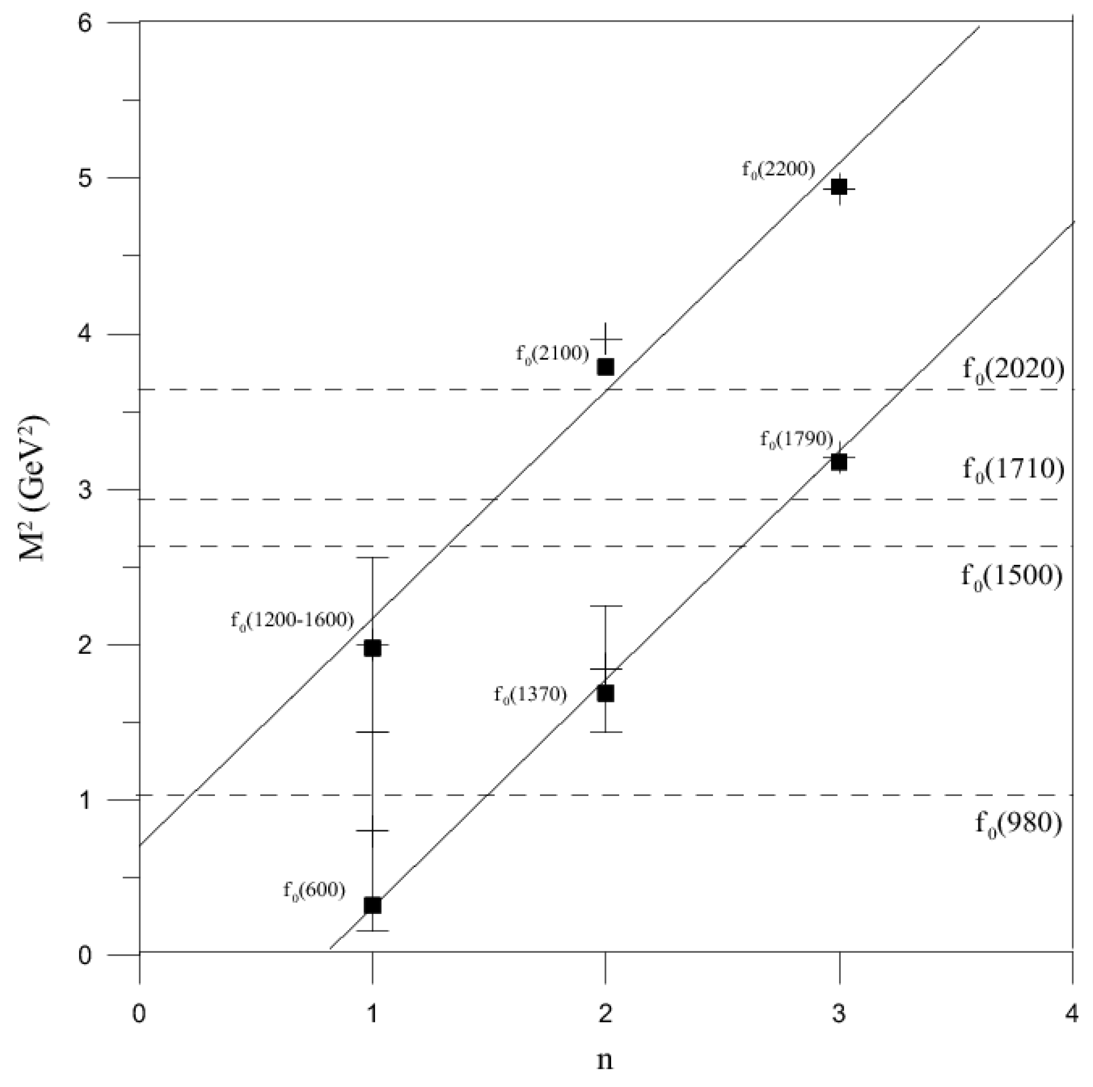
Let us now discussed some particular examples where four-quark structures could be present. First of all we center our attention on the light scalar-isoscalar mesons. In [18] scalar mesons below 2 GeV were studied in terms of the mixing of a chiral nonet of tetraquarks with conventional $q\overline{q}$ states using the scheme described in Section 2.8. We show in

Table 8. Mass, in MeV, and flavor dominant component of the light scalar-isoscalar mesons.

State	PDG	Mass	Flavor
$f_0(600)$	400−1200	568	$(n{\overline{n}}_{1P})$
$f_0(980)$	980±10	999	$(nn\overline{n}\overline{n})$
$f_0(1200-1600)$	1400±200	1299	$(s{\overline{s}}_{1P})$
$f_0(1370)$	1200−1500	1406	$(n{\overline{n}}_{2P})$
$f_0(1500)$	1507±5	1611	$(ns\overline{n}\overline{s})$
$f_0(1710)$	1714±5	1704	(glueball)
$f_0(1790)$	1790${}_{-30}^{+40}$	1782	$(n{\overline{n}}_{3P})$
$f_0(2020)$	1992±16	1902	$(ss\overline{s}\overline{s})$
$f_0(2100)$	2103±17	1946	$(s{\overline{s}}_{2P})$
$f_0(2200)$	2197±17	2224	$(s{\overline{s}}_{3P})$

results for the energies and dominant flavor component of the scalar-isoscalar mesons when considering also the mixing with a scalar glueball based on intuition from lattice QCD [30,31,32,33]. The results show a nice correspondence between theoretical predictions and experiment. This assignment suggests that there are four isoscalar mesons that are not dominantly $q\overline{q}$ states, they are the $f_0(980)$ (dominantly a $nn\overline{n}\overline{n}$ state), the $f_0(1500)$ (dominantly a $ns\overline{n}\overline{s}$ state), the $f_0(1710)$ (dominantly a glueball) and the $f_0(2020)$ (dominantly a $ss\overline{s}\overline{s}$ state). This is clearly seen in Figure 4 where we have constructed the two Regge trajectories associated to the isoscalar mesons. As it is observed the masses of the $f_0(600)$, $f_0(1200-1600)$, $f_0(1370)$, $f_0(1790)$, $f_0(2100)$, $f_0(2200)$ fit nicely in one of the two Regge trajectories, while those corresponding to the $f_0(980)$, $f_0(1500)$, $f_0(1710)$, $f_0(2020)$ do not fit for any integer value. The exception would be the $f_0(2020)$ that it is the orthogonal state to the $f_0(2100)$ having almost 50% of four-quark component. The glueball component is shared between the three neighboring states: 20 % for the $f_0(1370)$, 2 % for the $f_0(1500)$ and 76 % for the $f_0(1710)$. These results assigning the larger glueball component to the $f_0(1710)$ are on the line with [31,32] and differ from those of [34,35,36] concluding that the $f_0(1710)$ is dominantly $s\overline{s}$ and [37] supporting a low-lying glueball camouflaged within the $f_0(600)$ peak.

Another interesting scenario where four-quark states may help in the understanding of the experimental data is the open-charm meson sector [17,19,20]. The positive parity open-charm mesons present unexpected properties quite different from those predicted by quark potential models if a pure $c\overline{q}$ configuration is considered. We include in

Table 9. Probabilities (P), in %, of the wave function components and masses (QM), in MeV, of the open-charm and open-bottom mesons with $I=0$ (left) and $I=1/2$ (right) once the mixing between $q\overline{q}$ and $qq\overline{q}\overline{q}$ configurations is considered. Experimental data (Exp.) are taken from [6].

$\mathit{I}=0$						$\mathit{I}=1/2$
$J^P=0^{+}$			$J^P=1^{+}$			$J^P=0^{+}$
QM	2339	2847	QM	2421	2555	QM	2241	2713
Exp.	2317.8±0.6	−	Exp.	2459.6±0.6	$2535.4\pm 0.6$	Exp.	2352±50	−
P($cn\overline{s}\overline{n}$)	28	55	P($cn\overline{s}\overline{n}$)	25	$\sim 1$	P($cn\overline{n}\overline{n}$)	46	49
P($c{\overline{s}}_{1^{3}P}$)	71	25	P($c{\overline{s}}_{1^{1}P}$)	74	$\sim 1$	P($c{\overline{n}}_{1P}$)	53	46
P($c{\overline{s}}_{2^{3}P}$)	$\sim 1$	20	P($c{\overline{s}}_{1^{3}P}$)	$\sim 1$	98	P($c{\overline{n}}_{2P}$)	$\sim 1$	5
QM	5679	6174	QM	5713	5857	QM	5615	6086
P($bn\overline{s}\overline{n}$)	0.30	0.51	P($bn\overline{s}\overline{n}$)	0.24	$\sim 0.01$	P($bn\overline{n}\overline{n}$)	0.48	0.46
P($b{\overline{s}}_{1^{3}P}$)	0.69	0.26	P($b{\overline{s}}_{1^{1}P}$)	0.74	$\sim 0.01$	P($b{\overline{n}}_{1P}$)	0.51	0.47
P($b{\overline{s}}_{2^{3}P}$)	$\sim 0.01$	0.23	P($b{\overline{s}}_{1^{3}P}$)	$\sim 0.01$	0.99	P($b{\overline{n}}_{2P}$)	$\sim 0.01$	0.07

some results considering the mixing between $c\overline{q}$ configurations and four-quark states. Let us first analyze the nonstrange sector. The ${}^3{P}_0$ $c\overline{n}$ pair and the $cn\overline{n}\overline{n}$ have a mass of 2465 MeV and 2505 MeV, respectively. Once the mixing is considered one obtains a state at 2241 MeV with 46% of four-quark component and 53% of $c\overline{n}$ pair. The lowest state, representing the $D_0^{\ast }(2308)$, is above the isospin preserving threshold $D\pi$, being broad as observed experimentally. The mixed configuration compares much better with the experimental data than the pure $c\overline{n}$ state. The orthogonal state appears higher in energy, at 2713 MeV, with and important four-quark component.

Concerning the strange sector, the $D_{sJ}^{\ast }(2317)$ and the $D_{sJ}(2460)$ are dominantly $c\overline{s}$ $J=0^{+}$ and $J=1^{+}$ states, respectively, with almost 30% of four-quark component. Without being dominant, it is fundamental to shift the mass of the unmixed states to the experimental values below the $DK$ and $D^{\ast }K$ thresholds. Being both states below their isospin-preserving two-meson threshold, the only allowed strong decays to $D_s^{\ast }\pi$ would violate isospin and are expected to have small widths. This width has been estimated assuming either a $q\overline{q}$ structure [38,39], a four-quark state [40] or vector meson dominance [41] obtaining in all cases a width of the order of 10 keV. The second isoscalar $J^P=1^{+}$ state, with an energy of 2555 MeV and 98% of $c\overline{s}$ component, corresponds to the $D_{s1}(2536)$. Regarding the $D_{sJ}^{\ast }(2317)$, it has been argued that a possible $DK$ molecule would be preferred with respect to an $I=0$ $cn\overline{s}\overline{n}$ tetraquark, what would anticipate an $I=1$ $cn\overline{s}\overline{n}$ partner nearby in mass [42]. The present results support the last argument, namely, the vicinity of the isoscalar and isovector tetraquarks. However, the coupling between the four-quark state and the $c\overline{s}$ system, only allowed for the $I=0$ four-quark states due to isospin conservation, opens the possibility of a mixed nature for the $D_{sJ}^{\ast }(2317)$, the remaining $I=1$ pure tetraquark partner appearing much higher in energy. The $I=1$ $J=0^{+}$ and $J=1^{+}$ four-quark states appear above 2700 MeV and cannot be shifted to lower energies.

We finally tackled an interesting problem in tetraquark spectroscopy, the molecular or compact nature of four-quark bound states. This problem requires the determination of probabilities in non-orthogonal bases mathematically addressed in [24]. We show in

Table 10. Heavy-light four-quark state properties for selected quantum numbers. All states have positive parity and total orbital angular momentum $L=0$. Energies are given in MeV. The notation $M_1{M}_2{\mid }_{\ell }$ stands for mesons $M_1$ and $M_2$ with a relative orbital angular momentum ℓ. $P{[|\overline{3}3\rangle }_c^{12}{(|6\overline{6}\rangle }_c^{12})]$ stands for the probability of the $3\overline{3}(\overline{6}6)$ components given in Equation (5a) and $P[{\mid 11〉}_c({\mid 88〉}_c)]$ for the $11(88)$ components given in Equation (5b). $P_{MM}$, $P_{M{M}^{\ast }}$, and $P_{M^{\ast }{M}^{\ast }}$ have been calculated following the formalism of [24], and they represent the probability of finding two-pseudoscalar ($P_{MM}$), a pseudoscalar and a vector ($P_{M{M}^{\ast }}$) or two vector ($P_{M^{\ast }{M}^{\ast }}$) mesons.

$(\mathit{S},\mathit{I})$	(0,1)	(1,1)	(1,0)	(1,0)	(0,0)
Flavor	$cc\overline{n}\overline{n}$	$cc\overline{n}\overline{n}$	$cc\overline{n}\overline{n}$	$bb\overline{n}\overline{n}$	$bb\overline{n}\overline{n}$
Energy	3877	3952	3861	10395	10948
Threshold	$DD{\mid }_S$	$D{D}^{\ast }{\mid }_S$	$D{D}^{\ast }{\mid }_S$	$B{B}^{\ast }{\mid }_S$	$B_{1}B{\mid }_P$
${\Delta }_E$	+5	+15	$-76$	−217	$-153$
$P{[|\overline{3}3\rangle }_c^{12}]$	0.333	0.333	0.881	0.974	0.981
$P{[|6\overline{6}\rangle }_c^{12}]$	0.667	0.667	0.119	0.026	0.019
$P[{\mid 11〉}_c]$	0.556	0.556	0.374	0.342	0.340
$P[{\mid 88〉}_c]$	0.444	0.444	0.626	0.658	0.660
$P_{MM}$	1.000	−	−	−	0.254
$P_{M{M}^{\ast }}$	−	1.000	0.505	0.531	−
$P_{M^{\ast }{M}^{\ast }}$	0.000	0.000	0.495	0.469	0.746

some examples of results obtained for heavy-light tetraquarks. One can see how independently of their binding energy, all of them present a sizable octet-octet component when the wave function is expressed in the 5b coupling. Let us first of all concentrate on the two unbound states, ${\Delta }_E>0$, one with $S=0$ and one with $S=1$, given in Table 10. The octet-octet component of basis 5b can be expanded in terms of the vectors of basis 5c as explained in the previous section. Then, the probabilities are concentrated into a single physical channel, $MM$ or $M{M}^{\ast }$ [$MM$ stands for two identical pseudoscalar D (B) mesons and $M{M}^{\ast }$ for a pseudoscalar D (B) meson together with its corresponding vector excitation, $D^{\ast }$ ($B^{\ast }$)]. In other words, the octet-octet component of the basis 5b or 5c is a consequence of having identical quarks and antiquarks. Thus, four-quark unbound states are represented by two isolated mesons. This conclusion is strengthened when studying the root mean square radii, leading to a picture where the two quarks and the two antiquarks are far away, ${\langle x^2\rangle }^{1/2}\gg 1$ fm and ${\langle y^2\rangle }^{1/2}\gg 1$ fm, whereas the quark-antiquark pairs are located at a typical distance for a meson, ${\langle z^2\rangle }^{1/2}\le 1$ fm. Let us now turn to the bound states shown in Table 10, ${\Delta }_E<0$, one in the charm sector and two in the bottom one. In contrast to the results obtained for unbound states, when the octet-octet component of basis 5b is expanded in terms of the vectors of basis 5c, one obtains a picture where the probabilities in all allowed physical channels are relevant. It is clear that the bound state must be generated by an interaction that it is not present in the asymptotic channel, sequestering probability from a single singlet-singlet color vector from the interaction between color octets. Such systems are clear examples of compact four-quark states, in other words, they cannot be expressed in terms of a single physical channel.

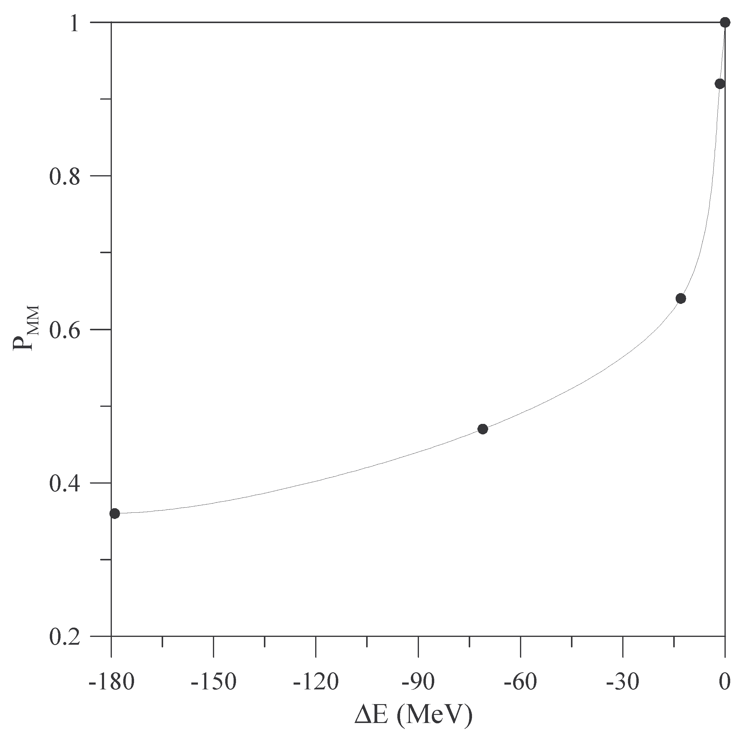
We have studied the dependence of the probability of a physical channel on the binding energy. For this purpose we have considered the simplest system from the numerical point of view, the $(S,I)=(0,1)$ $cc\overline{n}\overline{n}$ state. Unfortunately, this state is unbound for any reasonable set of parameters. Therefore, we bind it by multiplying the interaction between the light quarks by a fudge factor. Such a modification does not affect the two-meson threshold while it decreases the mass of the four-quark state. The results are illustrated in Figure 5, showing how in the ${\Delta }_E\to 0$ limit, the four-quark wave function is almost a pure single physical channel. Close to this limit one would find what could be defined as molecular states. When the probability concentrates into a single physical channel ($P_{M_1{M}_2}\to 1$) the system gets larger than two isolated mesons [20]. One can identify the subsystems responsible for increasing the size of the four-quark state. Quark-quark (${\langle x^2\rangle }^{1/2}$) and antiquark-antiquark (${\langle y^2\rangle }^{1/2}$) distances grow rapidly while the quark-antiquark distance (${\langle z^2\rangle }^{1/2}$) remains almost constant. This reinforces our previous result, pointing to the appearance of two-meson-like structures whenever the binding energy goes to zero.

6. Summary

We have presented a detailed analysis of the symmetry properties of a four-quark wave function and its solution by means of a variational approach for simple Hamiltonians. The numerical capability of the method has been analyzed. We have also emphasized the relevance of a correct analysis of the two-meson thresholds when dealing with the stability of four-quark systems. We have discussed the potential importance of four-quark structures in several different systems: the light scalar-isoscalar mesons and the open-charm mesons. We have also introduced the necessary ingredients to study the nature of four-quark bound states, distinguishing between molecular and compact four-quark states.

Although the present analysis has been performed by means of a particular quark interacting potential, the CQC model, the conclusions derived are independent of the quark-quark interaction used. They mainly rely on using the same hamiltonian to describe tensors of different order, two and four-quark components in the present case. When dealing with a complete basis, any four-quark deeply bound state has to be compact. Only slightly bound systems could be considered as molecular. Unbound states correspond to a two-meson system. A similar situation would be found in the two baryon system, the deuteron could be considered as a molecular-like state with a small percentage of its wave function on the $\Delta \Delta$ channel, whereas the $H-$dibaryon would be a compact six-quark state. When working with central forces, the only way of getting a bound system is to have a strong interaction between the constituents that are far apart in the asymptotic limit (quarks or antiquarks in the present case). In this case the short-range interaction will capture part of the probability of a two-meson threshold to form a bound state. This can be reinterpreted as an infinite sum over physical states. This is why the analysis performed here is so important before any conclusion can be made concerning the existence of compact four-quark states beyond simple molecular structures.

If the prescription of using the same hamiltonian to describe all tensors in the Fock space is relaxed, new scenarios may appear. Among them, the inclusion of many-body forces is particularly relevant. In [12,13] the stability of $QQ\overline{n}\overline{n}$ and $Q\overline{Q}n\overline{n}$ systems was analyzed in a simple string model considering only a multiquark confining interaction given by the minimum of a flip-flop or a butterfly potential in an attempt to discern whether confining interactions not factorizable as two-body potentials would influence the stability of four-quark states. The ground state of systems made of two quarks and two antiquarks of equal masses was found to be below the dissociation threshold. While for the cryptoexotic $Q\overline{Q}n\overline{n}$ the binding decreases when increasing the mass ratio $m_Q/m_n$, for the flavor exotic $QQ\overline{n}\overline{n}$ the effect of mass symmetry breaking is opposite. Others scenarios may emerge if different many-body forces, like many-body color interactions [43,44] or ’t Hooft instanton-based three-body interactions [45], are considered.

References

- Gell-Mann, M.A. Schematic model of baryons and mesons. Phys. Lett. 1964, 8, 214–215. [Google Scholar] [CrossRef]
- Jaffe, R.L. Multiquark hadrons.I.Phenomenology of Q2 mesons. Phys. Rev. D 1977, 15, 267–280. [Google Scholar] [CrossRef]
- Moinester, M.A. How to search for doubly charmed baryons and tetraquarks. Z. Phys. A 1996, 355, 349–362. [Google Scholar] [CrossRef]
- Zouzou, S.; Silvestre-Brac, B.; Gignoux, C.; Richard, J.M. Four quark bound states. Z. Phys. C 1986, 30, 457–468. [Google Scholar] [CrossRef]
- Heller, L.; Tjon, J.A. On the existence of stable dimesons. Phys. Rev. D 1987, 35, 969–974. [Google Scholar] [CrossRef]
- Amsler, C.; Doser, M.; Antonelli, M.; Asner, D.; Babu, K.S.; Baer, H.; Band, H.R.; Barnett, R.M.; Beringer, J.; Bergren, E.; et al. Review of Particle Physics. Phys. Lett. B 2008, 667, 1–1340. [Google Scholar] [CrossRef]
- Jaffe, R.L. Exotica. Phys. Rep. 2005, 409, 1–45. [Google Scholar] [CrossRef]
- Swanson, E.S. The new heavy mesons: A status report. Phys. Rep. 2006, 429, 243–305. [Google Scholar] [CrossRef]
- Klempt, E.; Zaitsev, A. Glueballs, hybrids, multiquarks: Experimental facts versus QCD inspired concepts. Phys. Rep. 2007, 454, 1–202. [Google Scholar] [CrossRef]
- Ader, J.P.; Richard, J.M.; Taxil, P. Do narrow heavy multiquark states exist? Phys. Rev. D 1982, 25, 2370–2382. [Google Scholar] [CrossRef]
- Ballot, J.L.; Richard, J.M. Four quark states in additive potentials. Phys. Lett. B 1983, 123, 449–451. [Google Scholar] [CrossRef]
- Vijande, J.; Valcarce, A.; Richard, J.-M. Stability of multiquarks in a simple string model. Phys. Rev. D 2007, 76, 114013:1–114013:5. [Google Scholar] [CrossRef]
- Ay, C.; Richard, J.M.; Rubinstein, J.H. Stability of asymmetric tetraquarks in the minimal-path linear potential. Phys. Lett. B 2009, 674, 227–231. [Google Scholar] [CrossRef]
- Quantum theory of angular momentum; Varshalovich, D.A.; Moskalev, A.N.; Khersonsky, V.K. (Eds.) World Scientific: Singapore, 1988. [Google Scholar]
- de Swart, J.J. The octet model and its Clebsch-Gordan coefficients. Rev. Mod. Phys. 1963, 35, 916–939. [Google Scholar] [CrossRef]
- Kaeding, T.A. Tables of SU(3) isoscalar factors. 1995. Available online: http://arxiv.org/abs/nucl-th/9502037 (accessed on 23 November 2009).
- Vijande, J.; Fernández, F.; Valcarce, A. Open-charm meson spectroscopy. Phys. Rev. D 2006, 73, 034002:1–034002:9. [Google Scholar] [CrossRef]
- Vijande, J.; Valcarce, A.; Fernández, F.; Silvestre-Brac, B. Nature of the light scalar mesons. Phys. Rev. D 2005, 72, 034025:1–034025:8. [Google Scholar] [CrossRef]
- Vijande, J.; Valcarce, A.; Fernández, F. B meson spectroscopy. Phys. Rev. D 2008, 77, 017501:1–017501:4. [Google Scholar] [CrossRef]
- Vijande, J.; Valcarce, A.; Fernández, F. A multiquark description of the DsJ(2860) and DsJ(2700). Phys. Rev. D 2009, 79, 037501:1–037501:4. [Google Scholar] [CrossRef]
- Vijande, J.; Valcarce, A.; Barnea, N. Exotic meson-meson molecules and compact four–quark states. Phys. Rev. D 2009, 79, 074010:1–074010:16. [Google Scholar] [CrossRef]
- Vijande, J.; Weissman, E.; Barnea, N.; Valcarce, A. Do bound states exist? Phys. Rev. D 2007, 76, 094022:1–094022:17. [Google Scholar] [CrossRef]
- Barnea, N.; Vijande, J.; Valcarce, A. Four-quark spectroscopy within the hyperspherical formalism. Phys. Rev. D 2006, 73, 054004:1–054004:11. [Google Scholar] [CrossRef]
- Vijande, J.; Valcarce, A. Probabilities in nonorthogonal bases: Four–quark systems. Phys. Rev. C 2009, 80, 035204:1–035204:10. [Google Scholar] [CrossRef]
- Valcarce, A.; Garcilazo, H.; Fernández, F.; González, P. Quark–model study of few–baryon systems. Rep. Prog. Phys. 2005, 68, 965–1042. [Google Scholar] [CrossRef]
- Vijande, J.; Fernández, F.; Valcarce, A. Constituent quark model study of the meson spectra. J. Phys. G 2005, 31, 481–506. [Google Scholar] [CrossRef]
- Valcarce, A.; Garcilazo, H.; Vijande, J. Constituent quark model study of light- and strange-baryon spectra. Phys. Rev. C 2005, 72, 025206:1–025206:9. [Google Scholar] [CrossRef]
- Garcilazo, H.; Vijande, J.; Valcarce, A. Faddeev study of heavy-baryon spectroscopy. J. Phys. G 2007, 34, 961–976. [Google Scholar] [CrossRef]
- Valcarce, A.; Garcilazo, H.; Vijande, J. Towards an understanding of heavy baryon spectroscopy. Eur. Phys. J. A 2008, 37, 217–225. [Google Scholar] [CrossRef]
- Bali, G.S. QCD forces and heavy quark bound states. Phys. Rep. 2001, 343, 1–136. [Google Scholar] [CrossRef]
- McNeile, C.; Michael, C. Mixing of scalar glueballs and flavor-singlet scalar mesons. Phys. Rev. D 2001, 63, 114503:1–114503:11. [Google Scholar] [CrossRef]
- Lee, W.; Weingarten, D. Scalar quarkonium masses and mixing with the lightest scalar glueball. Phys. Rev. D 2000, 61, 014015:1–014015:17. [Google Scholar] [CrossRef]
- Amsler, C.; Close, F.E. Evidence for a scalar glueball. Phys. Lett. B 1995, 353, 385–390. [Google Scholar] [CrossRef]
- Amsler, C. Further evidence for a large glue component in the f0(1500) meson. Phys. Lett. B 2002, 541, 22–28. [Google Scholar] [CrossRef]
- Amsler, C.; Close, F.E. Is f0(1500) a scalar glueball? Phys. Rev. D 1996, 53, 295–311. [Google Scholar] [CrossRef]
- Close, F.E.; Kirk, A. Scalar glueball-qq¯ mixing above 1 GeV and implications for lattice QCD. Eur. Phys. J. C 2001, 21, 531–543. [Google Scholar] [CrossRef]
- Vento, V. Scalar glueball spectrum. Phys. Rev. D 2006, 73, 054006:1–054006:7. [Google Scholar] [CrossRef]
- Godfrey, S. Testing the nature of the (2317)+ and DsJ(2463)+ states using radiative transitions. Phys. Lett. B 2003, 568, 254–260. [Google Scholar] [CrossRef]
- Bardeen, W.A.; Eichten, E.J.; Hill, C.T. Chiral multiplets of heavy-light mesons. Phys. Rev. D 2003, 68, 054024:1–054024:11. [Google Scholar] [CrossRef]
- Nielsen, M. DsJ+(2317)→Ds+π0 decay width. Phys. Lett. B 2006, 634, 35–38. [Google Scholar] [CrossRef]
- Colangelo, P.; de Fazio, F. Understanding DsJ(2317). Phys. Lett. B 2003, 570, 180–184. [Google Scholar] [CrossRef]
- Barnes, T.; Close, F.E.; Lipkin, H.J. Implications of a DK molecule at 2.32 GeV. Phys. Rev. D 2003, 68, 054006 (1–5). [Google Scholar] [CrossRef]
- Dmitrašinović, V. Cubic Casimir operator of SUC(3) and confinement in the nonrelativistic quark model. Phys. Lett. B 2001, 499, 135–140. [Google Scholar] [CrossRef]
- Dmitrašinović, V. Color SU(3) symmetry, confinement, stability, and clustering in the q2q2 system. Phys. Rev. D 2003, 67, 114007:1–114007:12. [Google Scholar] [CrossRef]
- ’t Hooft, G. Computation of the quantum effects due to a four-dimensional pseudoparticle. Phys. Rev. D 1976, 14, 3432–3450. [Google Scholar] [CrossRef]