Mixing Matrix Estimation of Underdetermined Blind Source Separation Based on Data Field and Improved FCM Clustering


College of Information and Communication Engineering, Harbin Engineering University, Harbin 150001, China
*
Author to whom correspondence should be addressed.
Symmetry 2018, 10(1), 21; https://doi.org/10.3390/sym10010021
Submission received: 3 November 2017
/
Revised: 2 January 2018
/
Accepted: 3 January 2018
/
Published: 9 January 2018
Abstract
:In modern electronic warfare, multiple input multiple output (MIMO) radar has become an important tool for electronic reconnaissance and intelligence transmission because of its anti-stealth, high resolution, low intercept and anti-destruction characteristics. As a common MIMO radar signal, discrete frequency coding waveform (DFCW) has a serious overlap of both time and frequency, so it cannot be directly used in the current radar signal separation problems. The existing fuzzy clustering algorithms have problems in initial value selection, low convergence rate and local extreme values which will lead to the low accuracy of the mixing matrix estimation. Consequently, a novel mixing matrix estimation algorithm based on data field and improved fuzzy C-means (FCM) clustering is proposed. First of all, the sparsity and linear clustering characteristics of the time–frequency domain MIMO radar signals are enhanced by using the single-source principal value of complex angular detection. Secondly, the data field uses the potential energy information to analyze the particle distribution, thus design a new clustering number selection scheme. Then the particle swarm optimization algorithm is introduced to improve the iterative clustering process of FCM, and finally get the estimated value of the mixing matrix. The simulation results show that the proposed algorithm improves both the estimation accuracy and the robustness of the mixing matrix.
1. Introduction
Blind Source Separation (BSS) is used to solve the mixing matrix estimation. It can extract the source signals from the observed signals under the condition that little priori knowledge of sources or channel is obtained except for the independence of signals. In recent years, as a popular signal processing method, it has been successfully applied to many fields, such as: voice signal processing [1], biomedical engineering [2], array signal processing [3], image processing [4], mechanical fault diagnosis [5] and so on. According to the different numbers of observed signals and sources, blind source separation can be divided into three cases including undetermined, normal and overdetermined. Among them, underdetermined blind source separation (UBSS) is most popular in the current research because it best fits the practical application.
Sparse results analysis (SCA) [6] is the most representative method in blind source separation. Its performance usually depends on the sparseness of the signal. However, many of the signals are not sparse in real applications, which require the sparsity of the signals to be increased by means of short-time Fourier transform (STFT), wavelet transform (WT) and other methods. In this paper, the sparse time-frequency representation of the signal is obtained by short-time Fourier transform and our work is mainly focused on the mixing matrix estimation of blind source separation [7,8]. Abrard and Deville [9] proposed a time–frequency ratio of mixtures (TIFROM) algorithm, but the algorithm requires the existence of an adjacent time–frequency domain in which only one source exists; Puigt and Deville [10] applied the TIFROM algorithm into delay mixing model. Arberet [11] proposed the direction estimation of mixing matrix (DEMIX) algorithm by extracting the time-frequency point when there is only one source signal. Arberet [12] then extended the DEMIX algorithm to the no echo mixing model, Kim and Yoo [13] also proposed a method of single source detection using the mixing matrix ratio in the time–frequency domain. The ratio is real when just one source signal exists, however, when two or more signals exist at that point, the ratio becomes plural. Dong [14] normalized the time–frequency coefficients of the observed signals; Xu [15] extends the single-source detection algorithm into image processing and realizes single-source detection in the Haar wavelet domain, but still has high complexity and sensitivivity to noise. For MIMO radar signals, the time–frequency overlap together with the low sparsity weaken the effect of the mentioned algorithms. Ai [16] proposed a method using high-order cumulants and tensor decomposition, however, the great influence of noise leads to low robustness. Guo [17] proposed a hybrid method based on single-source detection and data field dynamics clustering, but the process of seeking the potential point is too slow.
On the analysis above, we propose a single-source principal value of complex angular detection method based on the characteristics of MIMO radar signals. The orthogonal discrete frequency-coding waveforms (DFCW) are processed by the STFT transform. The influence of noisy and isolated points in the observed signal space is filtered out, which improves both the sparseness and linear clustering. Due to the fact that the fuzzy C-means algorithm is easy affected by initial clustering centers, a data field aided fuzzy C-means clustering algorithm is proposed. Firstly, a new clustering number selection scheme is designed by constructing data field of the observed data particles. Since FCM may be interpreted as an optimal problem, it could be integrated with particle swarm optimization (PSO). Secondly, we introduce PSO to improve the iterative clustering process of FCM. The simulation results show that the proposed method has improved accuracy of mixing matrix estimation.
This paper is organized as follows. In Section 2, we briefly introduce the model of MIMO radar signals. In Section 3, the detection method of single-source principal value of complex angular is described. In Section 4 and Section 5, a novel estimation method based on two-step preprocessing of fuzzy clustering is proposed. The experimental results are given in Section 6. Finally, some conclusions are given in Section 7.
2. Model of MIMO Radar Signals
In order to avoid mutual interference among the transmission channels, MIMO radar transmits the ideal orthogonal waveform through spatially distributed antennas, which mainly includes frequency division waveform and code segment waveform. Thanks to its strong anti-detection ability and simplicity of implementation, DFCW is commonly used in MIMO radar systems. The signal model has the following form
where N is the total number of pulses, the sub-pulse width, L is the number of sub-pulses in n-th signal; the l-th sub-pulse frequency of the n-th signal is , , the frequency coding sequence of the n-th signal is expressed as
It can be further formulated as a sequence
3. Detection Method Based on Single-Source Principal Value of Complex Angular
3.1. Model of Underdetermined Blind Source Separation
For MIMO radar systems, the observed signal obtained by the receiving antenna can be regarded as the weighted sum of the transmitted signals. When the number of receiving antennas is smaller than that of the transmitting antennas, the signal separation is in accordance with UBSS. And the UBSS linear instantaneous mixing model can be expressed as
where represents M observed signals, represents N source signals, represents order mixing matrix, is the k-th column vector of mixing matrix, and means additive white noise.
3.2. Single-Source Principal Value of Complex Angular Detection
STFT transform is carried out on both sides of the Equation (5) to obtain the mixing model in the time–frequency domain.
where and are complex coefficients after the short-time Fourier transform of observed and source signal at the time–frequency point , respectively. If there is only one source at the time point , Equation (5) will have the following form:
where and represent the real and imaginary parts of signal , respectively. In the complex plane, the angular is formed by the positive real axis and the vector Z. The vector Z is made up of and the origin of coordinates. It can be denoted as , then we can conclude . However, any complex number of vectors in the complex plane will have an infinite number of angles, so we take a value for that satisfies for the principal angular, representing the direction of the complex vector. From Equation (7) we can get:
that is, when only source acts, each channel signal has the same principal value of the complex angular, and is located on the same line in the complex plane. According to the above inference, the signal after STFT transformation is extracted by using Equation (8) as the constraint, consequently the directionality in frequency domain of the observed signal is more significant. But in the actual signal detection, the constraints of Equation (8) are too harsh and can be relaxed as:
where is the detection threshold, and when there is only one source , the signal detected by the complex angular principal value will be linearly distributed in the complex plane. The direction vectors of each line correspond to a column vector in the mixing matrix, respectively.
4. Mixing Matrix Estimation Based on Two-Step Preprocessing Fuzzy Clustering
4.1. Fuzzy C-Means Clustering Algorithm
FCM algorithm is an improvement of the early hard C-means clustering method. In this algorithm, data classification is achieved by minimizing the objective function. Compared with K-means clustering algorithm, the degree of membership defined in the range of is used to determine the degree of the element belonging to a cluster center in the cluster signal space.
Let represent n signals to be clustered in S-dimensional Euclidean space, where ’s eigenvector is denoted as . The signals have clustering centers with position . The objective function of FCM is shown below:
Among them, is the weighting index through which the fuzzy degree of the clustering can be adjusted. indicates the Euclidean distance of the k-th signal to the i-th clustering center. The partitioning matrix is indicated as . represents the membership degree of the signal to be clustered. Moreover, the membership relationship between the clustering signal and the set is expressed as . For , each membership degree has the following relationship:
The constraint condition is Equation (11). The purpose of clustering is to minimize the objective function, i.e., . We introduce the Lagrangian multiplier so the new objective function is constructed.
The membership degree and clustering center can be derived by the partial derivative of Equation (12).
The procedures for the FCM algorithm are as follows:
Step 1: Set the number of cluster centers , weighted index , iteration stop threshold , maximum iteration number , initial cluster center , and initialization iteration number to 0;
Step 2: Calculate the initial distance matrix ;
Step 3: The membership matrix is updated by Equation (13);
Step 4: The cluster center is updated by Equation (14), and the number of iterations is added one;
Step 5: Then the distance matrix is calculated again, and the objective function is calculated by Equation (10). If the result is smaller than the iteration stop threshold or exceeds the maximum iteration number, the algorithm terminates and outputs the result, otherwise it jumps to step 4.
The FCM algorithm requires setting the number of cluster centers and initializing the membership matrix. Equations (13) and (14) are acquired by the Lagrangian multiplier method to calculate the membership degree matrix and the value of the clustering center until reaching the terminal condition. The FCM algorithm is a kind of good soft clustering method, but the algorithm has two principal shortcomings: First, the number of clustering centers must be given in advance. For most of signals, however, the optimal clustering number is unknown; second, the algorithm is an optimization method based on gradient descent—essentially a local search algorithm which is sensitive to the initial value. The clustering center generated by random initialization can easily lead to a local extreme value problem in the clustering process.
4.2. Introduce Data Field to Select the Number of Cluster Centers
In view of the shortcomings of FCM, in this section, the theory of data field is proposed to estimate the number of clustering signals in advance. And then guide the subsequent steps.
This method treats the signals to be clustered as particles with mass in the multidimensional data space. The particles generate fields in the data space. As a result, they will produce forces on the other particles as well as the other particles will also produce the corresponding forces. The data space is denoted as , represents the set of particles in the data space. The theory of data potential field is augmented by the nuclear field concept in physics and the interaction of all particles forms a data field, which can be analytically modeled by a scalar potential function and a vector intensity function [18,19,20]. The Cartesian grid is used to divide the space, so the potential function of the point vector Z is given as the formula:
where is the Euclidean distance between the point vector and , satisfies the normalization condition , and is the radiation factor that controls the interacting distance between two particles.
The distribution of potential function can be given by the equipotential diagram of each plane projection in the coordinate system. The potential of a certain position in the graph and the intensity of the equipotential line are proportional to the intensity of the position distribution. In the data field space, the particle with the same clustering characteristics will show a distribution of concentric curve. The method can be used effectively to specify the default parameter of clustering centers.
4.3. Using the Particle Swarm Optimization Algorithm to Optimize the Clustering Center
The particle swarm optimization algorithm is a swarm intelligence algorithm inspired by the social behavior of the population. The PSO algorithm works with a population of possible solutions rather than a single individual. Assuming that the population size is denoted by . The position of i-th particle in the S-dimensional spaces can be expressed as . The velocity of i-th particle can be indicated as . Particle velocity can be dynamically adjusted by its own and companions’ experiences to optimize the precision of the search process. It indicates that if a particle discovers a promising solution, other particles will move toward to it and explore this region more extensively. In order to reduce the likelihood of the particle leaving the search place, the velocity of the particle is clamped to a maximum , when , make .
The quality of particles can be evaluated by the fitness function . In the process of single particle and whole particle iterations, two variables are defined to record the location of the maximum value of the fitness function. The position of the maximum value of fitness function in single particle iteration is called individual extremum, denoted as ; similarly the position in whole particle iteration is called the global extremum . In the iterative process, and can be continuously updated according to and .
In Equations (16) and (17), , , represents the time of current iteration, represents the inertia weight, represents cognitive and social factors respectively, are regarded as two random numbers. The termination condition is the iteration time has reached its maximum or the fitness value of global extremum satisfies the preset stop threshold. The output result is the highest fitness in the whole iteration process, that is, the global extreme value denoted as .
The particle swarm optimization algorithm is introduced to improve the iterative clustering process of FCM. The fuzzy C-means algorithm is a gradient descent based optimization algorithm. Compared with FCM, particle swarm optimization is a kind of population-based optimization algorithm. Through appropriate values of inertia weight, cognitive factor, social factor along with other parameters, PSO can search for more areas in the solution space of the objective function to be optimized. In this way, an improved accuracy of clusters and efficient method can be obtained.
5. Implementation Steps of the Improved Method
In order to overcome the shortcomings of the FCM algorithm mentioned in the first section, we introduce the particle swarm optimization algorithm to increase the randomness of the search process as well as increase the degree and uniformity of the initial solution space. By means of these, a better global search ability is obtained. To be specific, by combining the PSO algorithm with the FCM algorithm, the iterative updating process of the “membership degree matrix—clustering center” in the FCM algorithm is optimized by the PSO optimization process. The velocity and position of the iterative process is optimized by self and social cognition, breaking the shortcoming of lacking variety in the search direction, and ultimately enhancing the ability of global optimization.
The purpose of the FCM clustering algorithm is to get the minimum value of the objective function, as shown in Equation (10), whereas in the PSO algorithm, when the global optimal solution is searched, the fitness function obtains the maximum value. Therefore, the fitness evaluation of the particle can refer to the objective function of FCM and be improved as follows [21]:
where is a constant, is the membership degree matrix obtained by FCM algorithm iteratively and stands for the membership degree of sample belonging to cluster center .
In this paper, a mixing matrix estimation method based on data field aided fuzzy C-means clustering algorithm is proposed. By introducing a data field and particle swarm optimization algorithm, the effectiveness of the FCM algorithm can be improved. The implementation steps of the proposed clustering algorithm are as follows:
Step 1: The data field of the aliasing MIMO radar observed signals with single-source principal value of complex angular detection is obtained, and the number of the data center to be clustered is acquired by the equipotential graph, denoted by ;
Step 2: Initialize the parameters: represents the population size, the number of clusters is , stands for the weighting index, the cognitive and social parameters are expressed as and respectively. The inertia factor is denoted as , the maximum number of iterations is set as , the velocity upper limit to and the iteration stop threshold are indicated as and ;
Step 3: Initialize the population of particles and generate the initial population randomly;
Step 4: Initialize the membership degree matrix , and use single step FCM to calculate the set of initial clustering center;
Step 5: Initialize the value of fitness function by using Equation (18);
Step 6: The best judgment: The current fitness value of the particle is compared with its individual extremum , and if it is greater than , the current position is assigned to . Furthermore, the individual extremum of the particle is compared with the global extremum of the population, and if it is greater than , will be updated to the current position;
Step 7: Population evolution: According to Equations (16) and (17), we can acquire the velocity and position of the next generation of particles and produce a new generation of population to be new cluster centers;
Step 8: We can achieve FCM clustering by using the number and locations of clustering centers respectively obtained by the data field and PSO algorithm. The iteration times denoted as and the value of the optimal clustering center in the iter-th iteration can be obtained;
Step 9: If the number of iterations reaches or the fitness reaches the threshold, the global optimal solution and the current membership matrix can be obtained, meanwhile, the algorithm terminates; otherwise, returns to step 6.
6. Simulation Results and Analysis
In order to verify the effectiveness of the proposed method, this paper makes a comparative experiment with the hierarchical clustering, K-means clustering, and tensor decomposition methods. The computer hardware used in the experiment is configured as Intel (R) Pentium (R) CPU G3260 @ 3.30GHz, with 4GB memory, a Windows 7 operating system, and MATLAB 8.1.0.604 (R2013a, MathWorks, Natick, MA, USA) as the development environment.
6.1. Evaluation Criteria of Estimation Error
The normalized mean square error is chosen as the evaluation criterion of the mixing matrix estimation [14,22,23], which can be expressed as:
where and represent the elements in the original and estimated mixing matrix, respectively. The estimation accuracy of the mixing matrix will increase as the normalized mean square error decreases.
6.2. Simulation Procedures
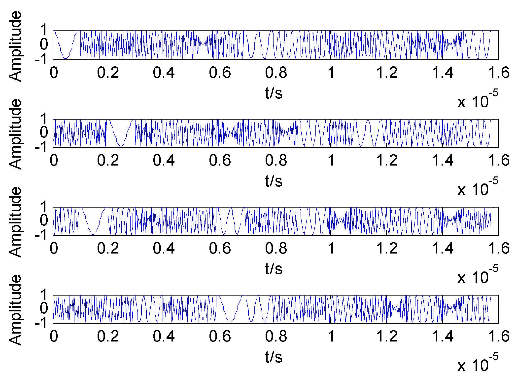
Suppose that the MIMO radar transmits four channel DFCW signals, i.e., . The pulse width is set to and the sub pulse width has a relation denoted as . The fundamental frequency is , let the bandwidth be and the sampling rate . Besides, is set to the default value of . After a series of experiments, the PSO algorithm has a population size of 20, and the number of cluster centers is equal to 4. The cognitive and social factors are set as 2 and the inertia weight is 0.3. Moreover, the maximum number of iterations is set to 20, the velocity upper limit is equal to 1.5, and the fitness function threshold . The value of the radiation factor in the data field is 0.1. The weighted index m in FCM algorithm is equal to 2, and the iteration stop threshold . The time domain waveform of the four transmission signals are shown in Figure 1.
The mixing matrix is chosen as the following form.
The mixing matrix is a -dimensional matrix, and three different noisy observed signals are received at the radar receivers. Figure 2 shows the distribution of the time–frequency points which belong to the three observed signals after STFT transformation. It can be seen that the time–frequency distribution in the figure is overlapped without obvious directionality.
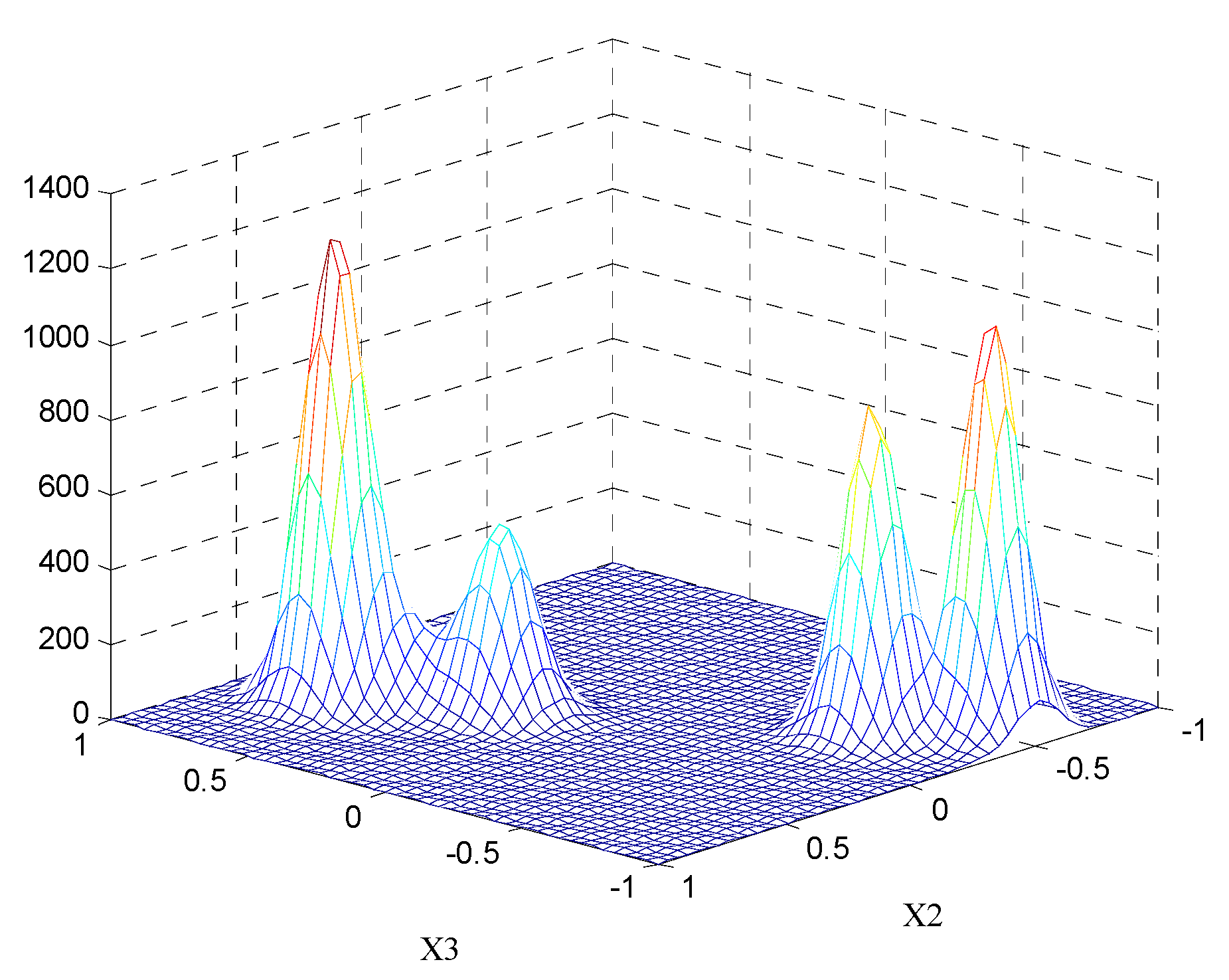
The observed signal is processed by a single-source principal value of complex angular detection. After that, the direction of the observed signal is obviously improved, but there are still many noisy and isolated points. As shown in Figure 3a, the measured data is regarded as particles in the data field and projected onto the unit hemisphere with a positive axis of . The potential value of the particles are calculated according to Equation (15). Using Cartesian grids, each dimension of data space is divided into 50 equal parts. The potential values at each grid point are obtained to establish the potential field. The projection of the potential field on three planes is given by Figure 3b–d, respectively. Figure 4 shows the three-dimensional potentiometric map on the X2–3 plane. In the diagram, the concentration of equipotential line and magnitude of the potential at a point are proportional to the density of the data points. By obtaining the extrema distribution of the potential points in each projection surface, initial values of the FCM algorithm can be provided. It can be determined that the number of clustering centers is equal to four.
The observed signal with obvious directivity after the test is iterated by the improved FCM clustering algorithm, and four global optimal convergence points are obtained. The spatial position vector of each convergence point corresponds to a column vector in the mixing matrix.
After the optimization of the cluster center by PSO and iterative clustering, the estimation result of the mixing matrix is obtained.
then the normalized mean square error of the mixing matrix estimation is calculated.
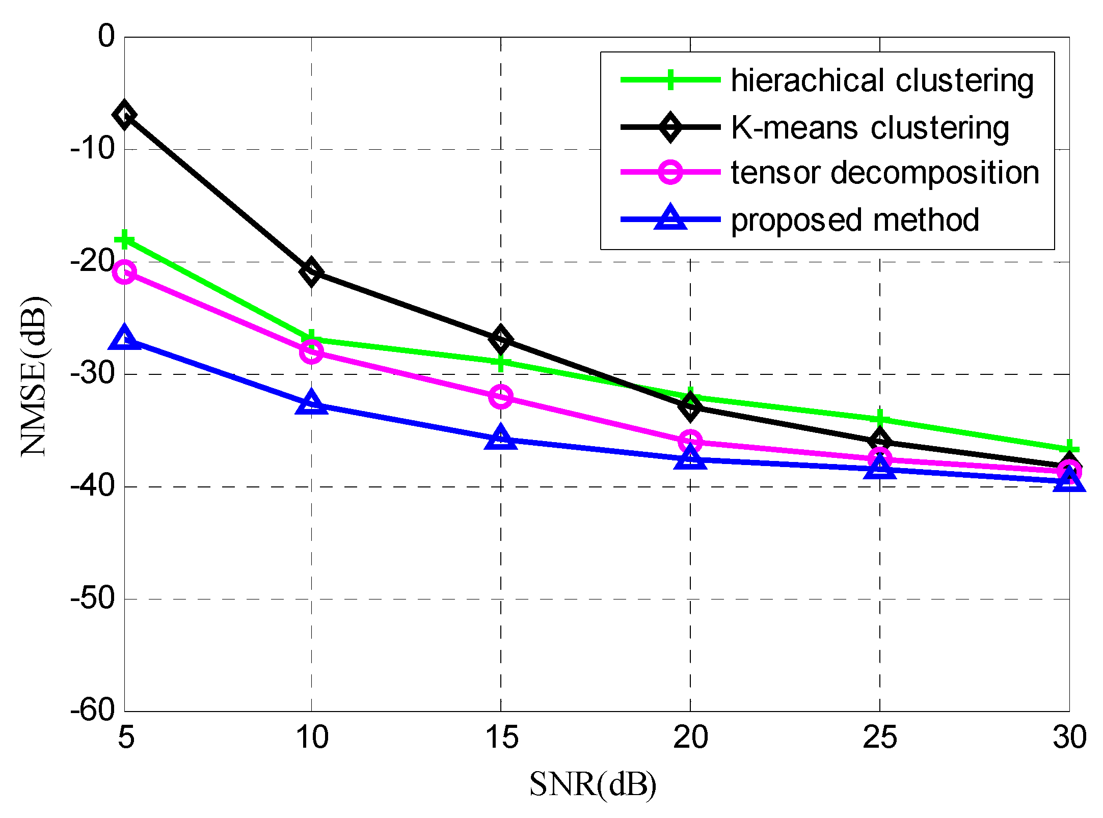
The method proposed in this paper is compared with the methods of hierarchical clustering, K-means clustering, and tensor decomposition. Figure 5 shows the averaged normalized mean square error obtained by 100 Monte Carlo independent tests when the signal-to-noise ratio (SNR) is in the range of for different methods. The simulation results show that with the increase of SNR, the estimation accuracy of each method will be improved. In this paper, due to the improvement of the iterative clustering process, the error value proposed by the method in question is the smallest, so a precise mixing matrix estimation can be achieved.
7. Conclusions
In order to improve the effect of mixing matrix estimation in the case of linear instantaneous mixture of MIMO radar DFCW signals, according to the time–frequency-sparse nature of the signal, firstly, the linear clustering characteristics are improved by single-source principal value of complex angular detection. Then, we propose a new selection scheme of clustering numbers based on the data field. And through the improved FCM clustering algorithm, mixing matrix can be estimated. The experimental results show that the proposed method can achieve higher estimation accuracy and robustness than other methods, which lays a good foundation for the accurate restoration of the MIMO radar source signals.
Acknowledgments
This work is supported by the National Key Research and Development Program of China (2016YFC0101700), the International S&T Cooperation Program of China (ISTCP) (No. 2015DFR10220), the Application Technology Research and Development of Heilongjiang Science and Technology Agency (No. GX16A007), National Natural Science Foundation of China (No. 61371172), the Application Technology Research and Development of Heilongjiang Science and Technology Agency (No. GC13A307), and the Fundamental Research Funds for the Central Universities (No. HEUCF1808).
Author Contributions
Qiang Guo and Chen Li conceived and designed the study. Chen Li and Guoqing Ruan performed the experiments. Chen Li wrote the paper. Qiang Guo, Chen Li and Guoqing Ruan reviewed and edited the manuscript. All authors read and approved the manuscript.
Conflicts of Interest
The authors declare no conflict of interest.
References
- Pedersen, M.S.; Wang, D. Two-microphone separation of speech mixtures. IEEE Trans. Neural Netw. 2008, 19, 475–492. [Google Scholar] [CrossRef] [PubMed] [Green Version]
- Abolghasemi, V.; Ferdowsi, S. Fast and incoherent dictionary learning algorithms with application to fMRI. Signal Image Video Process. 2015, 9, 147–158. [Google Scholar] [CrossRef]
- Xiang, W.; Huang, Z.; Zhou, Y. Semi-Blind Signal Extraction for Communication Signals by Combining Independent Component Analysis and Spatial Constraints. Sensors 2012, 12, 9024–9045. [Google Scholar]
- Aziz, M.A.E.; Khidr, W. Nonnegative matrix factorization based on projected hybrid conjugate gradient algorithm. Signal Image Video Process. 2015, 9, 1825–1831. [Google Scholar] [CrossRef]
- Wang, H.; Li, R.; Tang, G. A Compound Fault Diagnosis for Rolling Bearings Method Based on Blind Source Separation and Ensemble Empirical Mode Decomposition. PLoS ONE 2014, 9, e109166. [Google Scholar] [CrossRef] [PubMed]
- Hattay, J.; Belaid, S.; Lebrun, D. Digital in-line particle holography: Twin-image suppression using sparse blind source separation. Signal Image Video Process. 2015, 9, 1767–1774. [Google Scholar] [CrossRef]
- Romano, J.M.T.; Attux, R.; Cavalcante, C.C. Unsupervised Signal Processing: Channel Equalization and Source Seperation; CRC Press: Boca Raton, FL, USA, 2016. [Google Scholar]
- Naik, G.R.; Wang, W. Blind Source Separation; Springer: Berlin/Heidelberg, Germany, 2014. [Google Scholar]
- Abrard, F.; Deville, Y. A time-frequency blind signal separation method applicable to underdetermined mixtures of dependent sources. Signal Process. 2005, 85, 1389–1403. [Google Scholar] [CrossRef]
- Puigt, M.; Deville, Y. Time–frequency ratio-based blind separation methods for attenuated and time-delayed sources. Mech. Syst. Signal Process. 2005, 19, 1348–1379. [Google Scholar] [CrossRef] [Green Version]
- Arberet, S.; Gribonval, R.; Bimbot, F. A robust method to count and locate audio sources in a stereophonic linear anechoic mixture. In Proceedings of the IEEE International Conference on Acoustics, Speech and Signal Processing, ICASSP 2007, Honolulu, HI, USA, 15–20 April 2007. [Google Scholar]
- Arberet, S.; Gribonval, R.; Bimbot, F. A robust method to count and locate audio sources in a multichannel underdetermined mixture. IEEE Trans. Signal Process. 2010, 58, 121–133. [Google Scholar] [CrossRef] [Green Version]
- Kim, S.G.; Yoo, C.D. Underdetermined blind source separation based on subspace representation. IEEE Trans. Signal Process. 2009, 57, 2604–2614. [Google Scholar]
- Dong, T.; Lei, Y.; Yang, J. An algorithm for underdetermined mixing matrix estimation. Neurocomputing 2013, 104, 26–34. [Google Scholar] [CrossRef]
- Xu, J.; Yu, X.; Hu, D. A fast mixing matrix estimation method in the wavelet domain. Signal Process. 2014, 95, 58–66. [Google Scholar] [CrossRef]
- Ai, X.F.; Luo, Y.J.; Zhao, G.Q. Underdetermined blind separation of radar signals based on tensor decomposition. Syst. Eng. Electron. 2016, 38, 2505–2509. [Google Scholar]
- Guo, Q.; Ruan, G.; Nan, P. Underdetermined Mixing Matrix Estimation Algorithm Based on Single Source Points. Circuits Syst. Signal Process. 2017, 36, 4453–4467. [Google Scholar] [CrossRef]
- Giachetta, G.; Mangiarotti, L.; Sardanashvily, G. Advanced Classical Field Theory; World Scientific: Singapore, 2009. [Google Scholar]
- Kante, B.; Germain, D.; De Lustrac, A. Near field imaging of refraction via the magnetic field. Appl. Phys. Lett. 2014, 104, 021909. [Google Scholar] [CrossRef]
- Li, D.; Wang, S.; Gan, W. Data Field for Hierarchical Clustering. Int. J. Data Warehous. Min. 2011, 7, 43–63. [Google Scholar]
- Filho, T.M.S.; Pimentel, B.A.; Souza, R.M.C.R. Hybrid methods for fuzzy clustering based on fuzzy c-means and improved particle swarm optimization. Expert Syst. Appl. Int. J. 2015, 42, 6315–6328. [Google Scholar] [CrossRef]
- Sun, J.; Li, Y.; Wen, J. Novel mixing matrix estimation approach in underdetermined blind source separation. Neurocomputing 2016, 173, 623–632. [Google Scholar] [CrossRef]
- Reju, V.G.; Koh, S.N.; Soon, I.Y. An algorithm for mixing matrix estimation in instantaneous blind source separation. Signal Process. 2009, 89, 1762–1773. [Google Scholar] [CrossRef]
Figure 1.
Time domain waveform of transmitted signals.

Figure 2.
The time–frequency scatter plot of transmitted signals.
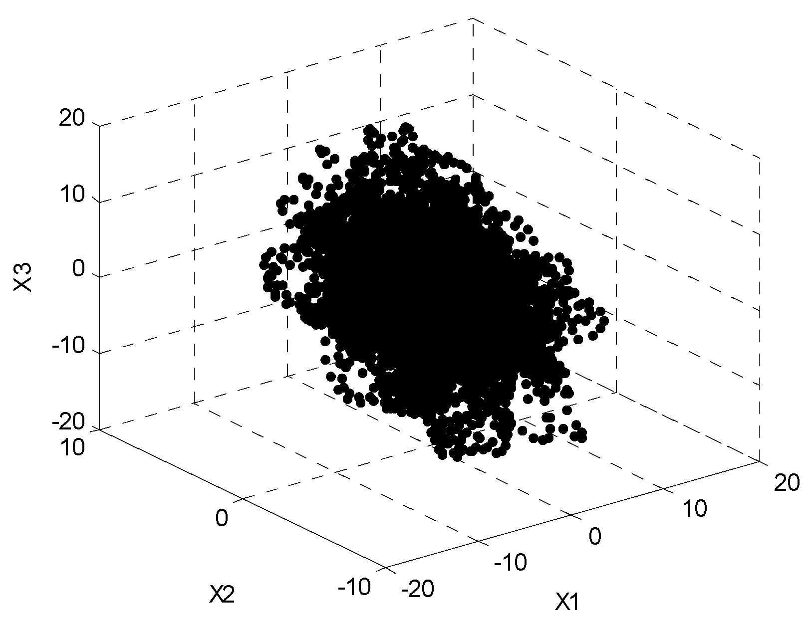
Figure 3.
(a) Distribution map on unit-positive hemispherical; (b) Potentiometric map on the X1–X2 plane; (c) Potentiometric map on the X1–X3 plane; (d) Potentiometric map on the X2–X3 plane.
Figure 3.
(a) Distribution map on unit-positive hemispherical; (b) Potentiometric map on the X1–X2 plane; (c) Potentiometric map on the X1–X3 plane; (d) Potentiometric map on the X2–X3 plane.
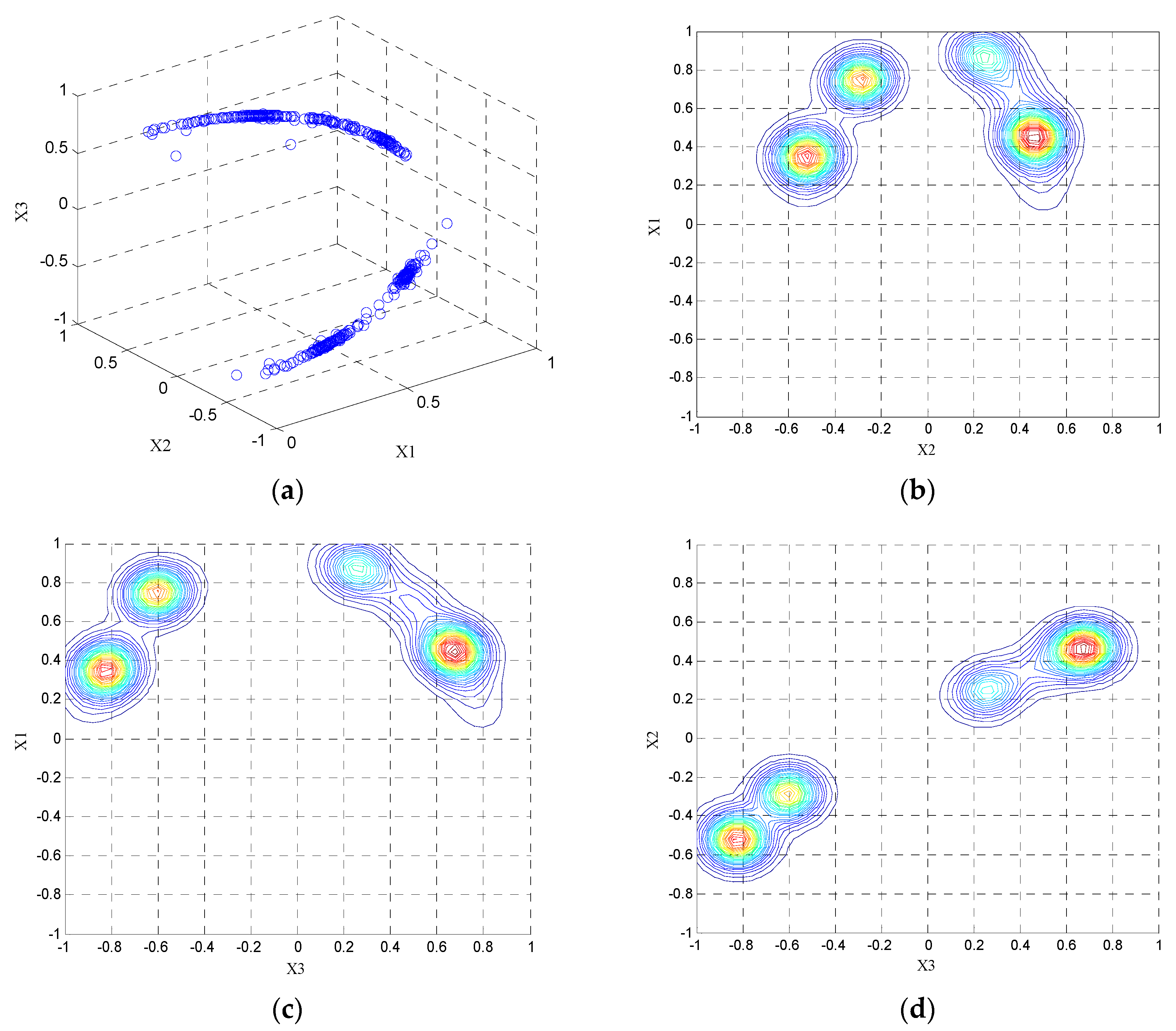
Figure 4.
Three-dimensional potentiometric map on the X2–X3 plane.

Figure 5.
Comparison chart of NMSE.

© 2018 by the authors. Licensee MDPI, Basel, Switzerland. This article is an open access article distributed under the terms and conditions of the Creative Commons Attribution (CC BY) license (http://creativecommons.org/licenses/by/4.0/).
Share and Cite
MDPI and ACS Style
Guo, Q.; Li, C.; Ruan, G. Mixing Matrix Estimation of Underdetermined Blind Source Separation Based on Data Field and Improved FCM Clustering. Symmetry 2018, 10, 21. https://doi.org/10.3390/sym10010021
AMA Style
Guo Q, Li C, Ruan G. Mixing Matrix Estimation of Underdetermined Blind Source Separation Based on Data Field and Improved FCM Clustering. Symmetry. 2018; 10(1):21. https://doi.org/10.3390/sym10010021
Chicago/Turabian StyleGuo, Qiang, Chen Li, and Guoqing Ruan. 2018. "Mixing Matrix Estimation of Underdetermined Blind Source Separation Based on Data Field and Improved FCM Clustering" Symmetry 10, no. 1: 21. https://doi.org/10.3390/sym10010021
Note that from the first issue of 2016, this journal uses article numbers instead of page numbers. See further details here.