How Symmetric Are Real-World Graphs? A Large-Scale Study

Karlsruhe Institute of Technology, Institute of Information Systems and Marketing, Kaiserstr. 12, 76131 Karlsruhe, Germany
*
Author to whom correspondence should be addressed.
Symmetry 2018, 10(1), 29; https://doi.org/10.3390/sym10010029
Submission received: 22 December 2017
/
Revised: 9 January 2018
/
Accepted: 10 January 2018
/
Published: 16 January 2018
Abstract
:The analysis of symmetry is a main principle in natural sciences, especially physics. For network sciences, for example, in social sciences, computer science and data science, only a few small-scale studies of the symmetry of complex real-world graphs exist. Graph symmetry is a topic rooted in mathematics and is not yet well-received and applied in practice. This article underlines the importance of analyzing symmetry by showing the existence of symmetry in real-world graphs. An analysis of over 1500 graph datasets from the meta-repository networkrepository.com is carried out and a normalized version of the “network redundancy” measure is presented. It quantifies graph symmetry in terms of the number of orbits of the symmetry group from zero (no symmetries) to one (completely symmetric), and improves the recognition of asymmetric graphs. Over 70% of the analyzed graphs contain symmetries (i.e., graph automorphisms), independent of size and modularity. Therefore, we conclude that real-world graphs are likely to contain symmetries. This contribution is the first larger-scale study of symmetry in graphs and it shows the necessity of handling symmetry in data analysis: The existence of symmetries in graphs is the cause of two problems in graph clustering we are aware of, namely, the existence of multiple equivalent solutions with the same value of the clustering criterion and, secondly, the inability of all standard partition-comparison measures of cluster analysis to identify automorphic partitions as equivalent.
1. Introduction
The analysis and understanding of the effects of symmetry has been a guiding principle in physics since the beginning of the 20th century [1]. The investigation of symmetry in network analysis—besides the area of (applied) math—seems not as far developed and depends on the field of research. Especially in chemistry, the recognition of graph symmetry plays a role, as the structure of molecules can be modeled with graphs and the distinction of molecular structures (i.e., checking for (non-) isomorphism) is of great interest [2]. This has also led to entropy-based measures, not only applicable in chemistry but also in the fields of biology, sociology and psychology [3,4].
The study of graph symmetries has been a field of research for many years [5]. Two graphs are said to be isomorphic if there exists a bijection of the set of nodes so that one graph equals the other under the transformation of the bijection. If bijections from a graph to itself besides the trivial identity bijection exist, a graph is symmetric and this symmetry is captured by the graph’s automorphism group. The formal details will be introduced in Section 2. Both problems (graph isomorphism—GI, and graph automorphism—GA) are not in and thus not easy to solve in general. For GI it is even unclear whether it is in (the complexity class of “nondeterministic polynomial-time complete” problems, often informally referred to as the class of the hardest problems to solve) [6]. Either way, efficient algorithms exist [7,8,9,10] and the latest research gathers momentum in lowering the theoretical worst-case complexity [11,12] (still under review as of September 2017).
The strict symmetry definition in terms of topological symmetry is not the only way to characterize graph symmetries, as Garlaschelli et al. [13] show in their review. Nonetheless, we concentrate on strict symmetry for the rest of this paper. Erdős and Rényi [14] showed that random graphs tend to be asymmetric, that is, there do not exist automorphisms that map nodes onto nodes by preserving the graph’s structure. In contrast, for graphs that are the result of structures (or processes, social relations, etc.) that occur in reality—thus the name real-world graphs—it has been shown that they do not obey the law of pure randomness [15] but follow other principles, such as the power law probability distribution [16]. Therefore, the conclusion “symmetries in real-world graphs are unlikely” is false without further evidence. Several empirical investigations on the actual symmetry of complex/real-world networks already exist [10,17,18], with an emphasis on [19], but all these publications have in common that only a very small selection of graphs (about 25 maximal) was taken into account. A theoretical overview of symmetry in complex networks is given by Garrido [20]. Our contribution is to undertake a symmetry analysis on a much larger scale, utilizing graph data from the meta-repository networkrepository.com (http://www.networkrepository.com, last accessed 28 August 2017) [21].
The rest of this article is organized as follows: We formally define graph symmetry and other concepts in Section 2 and will then describe the procedure we carried out (Section 3). We end by presenting the obtained results (Section 4) and by giving a short outlook (Section 6) and conclusion (Section 5). Our Appendices contain additional details on the analysis (Appendix A), a theorem and a proof concerning the redundancy measure we present in Section 3 (Appendix B), some more result diagrams (Appendix C), and additional results (Appendix D).
2. Definition of Graph Symmetry
A graph G is a set of nodes (or vertices) V and a set of edges E that together form a topological structure . We define (w. l. o. g.) and , which is a simple graph (no self-loops, no edge weights, no multiple edges) with at most edges. This definition makes nodes distinguishable by their label . Furthermore, it is sufficient to consider only connected graphs. That is, no two nodes exist that cannot be reached by a sequence of nodes connected by an edge (a path). For brevity, we write edges as where appropriate.
Let us now formally define isomorphisms and automorphisms of graphs. Both are bijections that map nodes onto nodes by preserving topology. These bijections are permutations of the node set and we write them as cycles. Two graphs and are isomorphic iff with and the mapping — the image of applied on u. If , is an automorphism of the graph G. The identity mapping is always a (trivial) automorphism. For any bijection there naturally exists an inverse and the composition of both bijections is . The set of all automorphisms that exist for a graph G form the group that obeys the four group properties:
- Identity: .
- Inverses: and .
- Closure: .
- Associativity: .
A subset of automorphisms that yields when applying the above properties is called a generating set; the elements are generators. If contains only , it is said to be trivial and G is said to be asymmetric. The group size is simply the number of elements (permutations) and if , G is symmetric.
The automorphism group induces equivalence classes of the nodes of the graph, which are called orbits. An orbit of a node u is defined as . That is, all nodes that can be mapped onto each other are on the same orbit and the set of all orbits is a non-overlapping partition of V. The number of nodes on an orbit defines its length. A node with an orbit length of one is said to be fixed by .
The definition of automorphisms can easily be extended to non-simple graphs. If E is allowed to be a multiset, multiple edges are possible. If edges are expressed by ordered tuples instead of sets, the graph is directed. In both cases, the above definitions are directly applicable. If we interpret the requirement as a constraint that limits the set of all possible bijections , we can think of further constraints, for example, induced by a function that assigns weights to edges. So for the automorphism of a weighted graph, additionally must hold.
The group containing all bijections of the above form is called the symmetric group of V and is denoted . The group is called a subgroup, denoted . The more constraints are introduced to define an automorphism of a graph, the smaller the subgroup becomes. Let, for example, G be a simple graph with the automorphism group and be the same graph with an additional edge weight function, then . This consequence will become important in Section 3.
3. Description of the Graph Symmetry Analysis Procedure
The analysis procedure can be divided into several independent steps. Each step is automated by implementing a Python script:
- Retrieval of graph metadata from networkrepository.com (includes the download link to the actual dataset).
- Selection of the datasets to download (by file size).
- Retrieval of the actual datasets (compressed zip-archives).
- Loading, selection and transformation of the graph data to perform the symmetry computations.
- Calculation of statistics and their analysis (discussed in Section 4).
The crucial part of the analysis is the computation of generators of the automorphism group of each graph in step four. The normalized network redundancy (introduced in Section 3.5) is based on the number of orbits that can be deduced from the generators.
We will give a brief overview of each of these steps before we present and interpret the results. Additional aspects and details are described in Appendix A. The analysis was performed in February/March 2017, thus all information we give was up-to-date at that time.
3.1. The Data Repository: networkrepository.com
networkrepository.com [21] is a platform that advertises to be “[t]he first interactive data and network repository with real-time analytics” (http://www.networkrepository.com, last accessed 28 August 2017). It lists about 3900 datasets and provides several (sometimes approximate) characteristics for each dataset. The datasets are grouped into classes of origin (for example, “Biological Networks”, “Cheminformatics”, “Social Networks”, etc.) with the smallest class containing less than 10 networks, the largest (“Miscellaneous Networks”) more than 2500. A striking advantage of this repository is that it also contains many datasets which can be found in other sources (for example, the one of GEPHI [22] (https://github.com/gephi/gephi/wiki/Datasets, last accessed 29 August 2017), SNAP [23] or the DIMACS challenges [24], 10th DIMACS challenge (http://dimacs.rutgers.edu/Challenges/, last accessed 29 August 2017)). This allowed us to easily retrieve many datasets at once without the need to combine several sources and—potentially—different data formats. A flaw of using this source of data is the presence of datasets that are not actual real-world graphs, as the discussion of the results will show.
3.2. Data Download Selection
We decided to download all datasets with a (compressed) size of about 70 megabytes or less. Even if this sounds to be very far away from “big data”, considering nodes, the largest network in our sample consisted of 11,950,757 nodes and m = 12,711,603 edges. Looking at the edges, the largest graph in the sample has nodes and m = 25,165,784 edges. The obvious reason for this is that large graphs also have, encoded as a list of edges, a fairly low consumption of disk space—mainly depending on the number of edges. Certainly, not the disk space but the algorithmic complexity of obtaining the automorphism group of a graph, which normally increases at least linearly with the size of the graph, was crucial for this decision. In the end, we downloaded a total of 3015 datasets with an overall compressed size of 11.5 gigabytes.
3.3. Data Formats
The downloaded graphs are encoded in either one of two plain-text data formats:
The former is a matrix format that contains the actual matrix format information in the first line, and each following line encodes a matrix entry by position. The latter also begins with some meta-information in the first lines, followed by a list of edges (one per line).
It is of high importance to understand how the graph data is encoded, to decide which datasets to choose (simple graphs) and which to exclude (all other graphs) from the symmetry analysis.
3.4. Data Analysis Selection
As stated in our introduction, we focus on simple graphs. One of the reasons is that saucy [10], which we used to compute generating sets for the automorphism groups, cannot handle weighted graphs. networkrepository.com also contains datasets of dynamic networks that change over time. These should be excluded as it is not clear which state of the network is the one to analyze (start, end, average, every state from start to end, …?). Some other datasets consist of disconnected components which we also excluded from further processing.
Often, for example, [19], non-simple graphs are “simplified” by removing multiple edges, loops and edge weights, and replacing edge 2-tuples (directed) by edge 2-sets (undirected). We refrained from doing so as this simplification is likely to “add” symmetry that is actually not present in the original version of the graph (see the example in Figure 1). This is why we view these properties as constraints in Section 2 that restrict the set of automorphisms of a graph. Sometimes, some of these simplifications may be appropriate, but as we want to analyze exact symmetry, this one in particular is not. However, additional results for simplified graphs are presented in Appendix D.
Another issue we had to face was the existence of duplicates, which had several causes: Sometimes the same graph was put into different classes, sometimes a graph existed in the same class but under a slightly different name. In the end, from the 3015 downloaded datasets, a total of 1805 were sorted out (non-simple graphs) and another 277 graphs were disconnected and thus also excluded from the analysis. From the remaining 933 graphs, 31 were identified as duplicates having a different name after manual postprocessing. Most of these duplicates were part of the “DIMACS10” class, which contains datasets from a graph clustering and partitioning challenge held in 2012 (http://www.cc.gatech.edu/dimacs10/, last accessed 30 August 2017). We found all graphs of this special class to be also contained in one of the other classes. Some other graphs were also duplicated in different classes, but only few were duplicated in the same class.
All in all, we decided to remove all duplicates from our analyses on the complete dataset but to keep duplicates for the analyses on the class level to prevent a bias within classes.
3.5. Data Analysis Procedure
Finally, we describe which characteristics were computed for each graph. As we laid our focus on the analysis of symmetry, it was most important to compute the automorphism group of each graph. To achieve this, we utilized saucy [10]. Calling saucy with a simple graph as input returns the size of the group, the number of permutations that generate the group, and some other information (sum of the permutation’s support, depth and number of nodes of the search tree), which we do not use further. Actually, we did call saucy from Python and additionally computed the orbit partition (see the details in Appendix A).
As the size of an automorphism group grows exponentially fast with the degree of symmetry, the number representing size is split into two values a and b so that . However, the group size as an absolute value is not a very intuitive way to describe how symmetric a graph actually is. Think, for example, of the case of a graph that has 100 nodes and 15 of them can be mapped onto each other in any way, while all others are fixed. The group of this graph is equivalent to with (see also the results in the last column of Table 1).
MacArthur et al. [19] introduced a relative measure for the degree of symmetry, which they call “network redundancy”:
It is much more robust against how nodes on the same orbit can be mapped onto each other, because an orbit only contains the information that nodes can be mapped onto each other. We believe a better measure is
the normalized (network) redundancy. It perfectly captures the asymmetric case () as well as the completely symmetric case () and better correlates with the name “redundancy”. A completely symmetric graph (a transitive graph) has a normalized redundancy of 1 (100%) as all nodes are equivalent and therefore redundant. Moreover, asymmetric graphs of different size can be compared because the normalized redundancy is 0 and not (for large n). The normalized redundancy is of course only defined for graphs with more than one node, but in practice this is no restriction at all.
4. Results
The main goal of this article is to provide further evidence of symmetries that exist in real-world graphs. Table 1 shows a summary of some basic statistics of the datasets. The last two columns contain symmetry information obtained by saucy. In the end, we analyzed a total of 902 different graphs (duplicates already removed). As discussed previously, the size of the automorphism group is not a good measure for the degree of symmetry. Nonetheless, it can be seen that 75% of the analyzed graphs have a very small group size. In total, 272 of the 902 graphs are asymmetric, which means about 70% contain symmetries.
From the median values (50%) of the first two columns in Table 1 it can be seen that many analyzed graphs are quite small. However, also relatively larger graphs were part of the analysis, as the maximum values show. Many graphs seem to have a modular structure which is not unusual for real-world graphs [16] (see Section 3.7; higher values of Q imply a more modular structure).
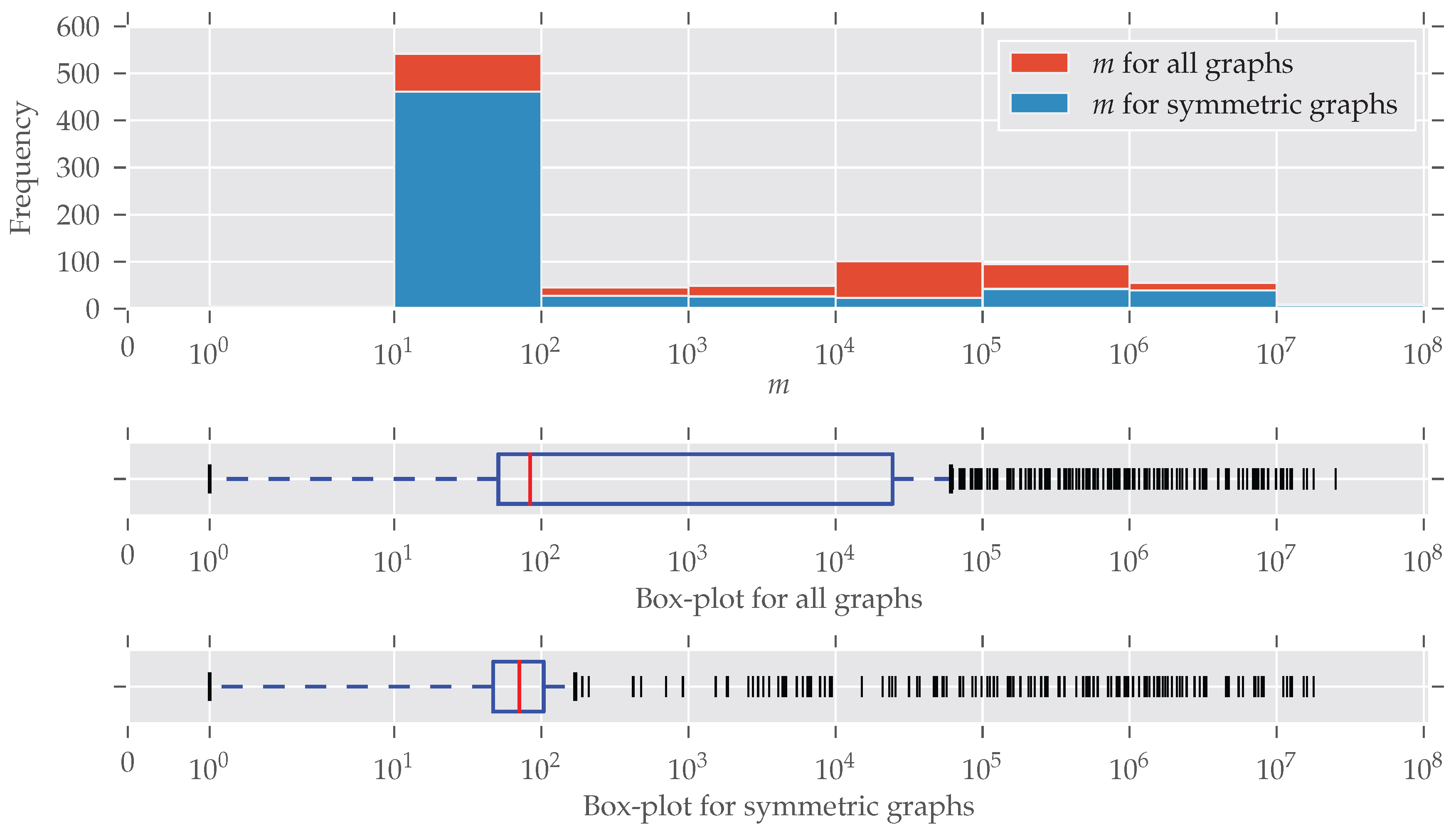
In Figure 2 the distribution of the number of edges is plotted (note the log-scaled x-axis and bin size). Symmetries are found for every size of graphs; only for larger graphs () do symmetries seem to be under-represented. An explanation for this is the existence of many graphs that are generated following some random graph model and, therefore, are asymmetric. The details of this are described below. The plot for the number of nodes n looks similar, so we decided to put it in Appendix C (Figure A2). More than half of the graphs contain between 10 and 100 edges. This “bias” emerges from the high number of graphs from the “chem” class, which is very large (over 570 datasets) and consists predominantly of graphs with less than 100 edges.
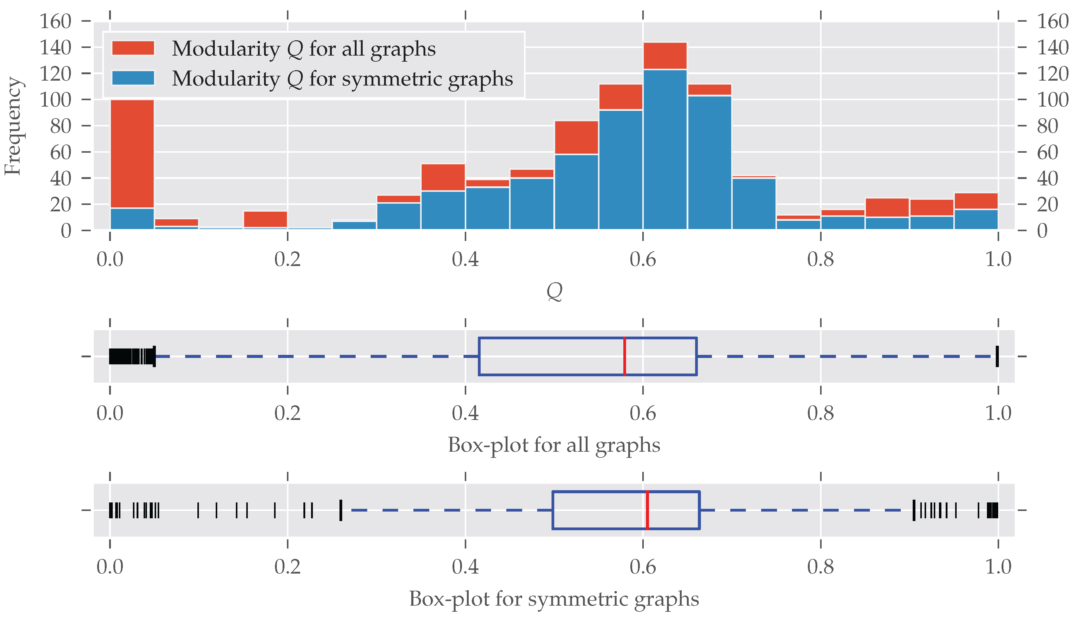
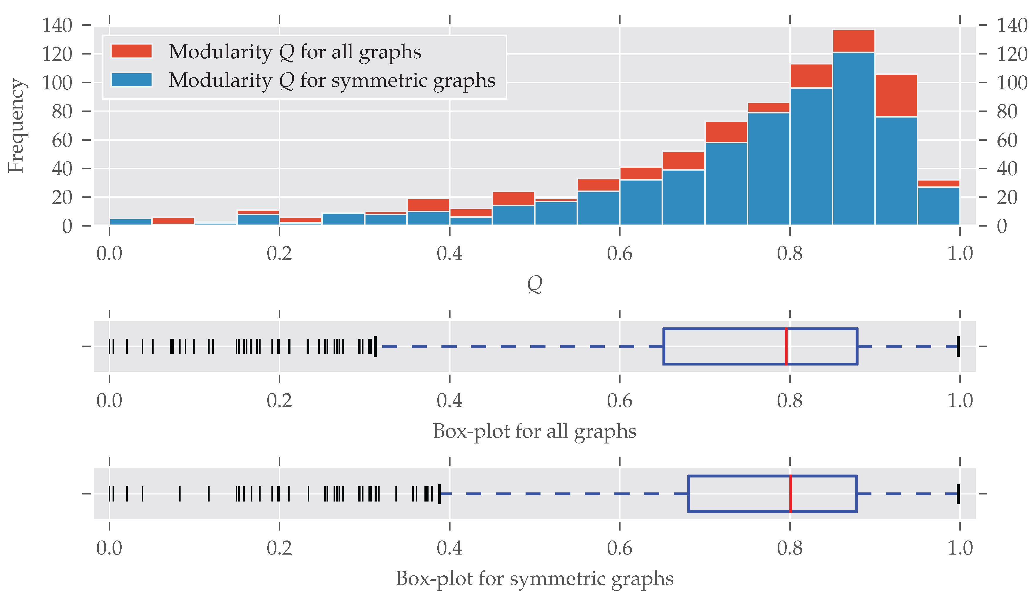
As for the graphs’ size, modular graphs often do contain symmetries, as Figure 3 shows. Which modularity values for a partition are interpreted as “good” largely depends on the graph’s size. For example, the Karate network [29] is relatively small (, ) and the optimal modularity maximizing partition yields a value of nearly 0.42 [27].
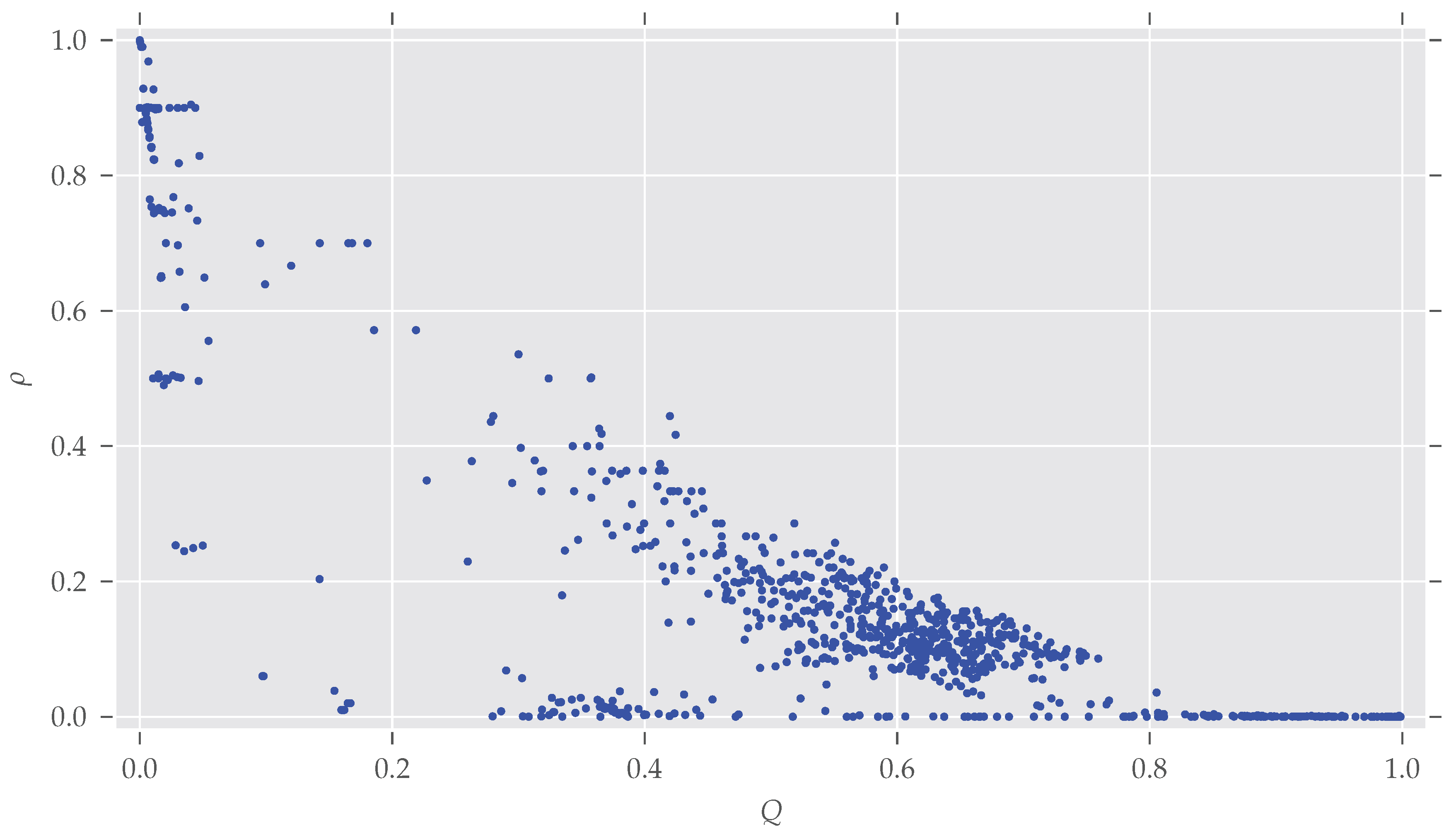
A bit surprising is the large fraction of asymmetric graphs with very low modularity (<0.05): Normally, maximum modularity decreases when the density of the network—that is, the number of edges compared to the maximal possible number of edges —increases (see Figure A3). That is because with an increasing number of edges it becomes impossible to partition the set of nodes in a way that nodes within clusters are more connected to each other than to nodes in different clusters (for details see [28,30]). On the other hand, a graph is likely to become symmetric if more and more edges are added, which increases its density [31].
Indeed, all the graphs with have a very high average density of (std ). By directly investigating the analyzed datasets we found out that most of these low-modularity low-symmetry graphs come from the dimacs and bhoslib classes. The dimacs class contains data from the second DIMACS challenge, which was about “Maximum Clique, Graph Coloring, and Satisfiability” (http://dimacs.rutgers.edu/Challenges/, last accessed 29 August 2017). These graphs were generated, thus no actual real-world networks. The bhoslib class is discussed below. A third group of graphs were part of the misc class and have names G1, G2 and so on. These are also generated as described by Helmberg and Rendl [32]—most of them following a random model. As a consequence, these findings explain the large amount of highly non-modular and asymmetric graphs in Figure 3. It is also important to note that very non-modular graphs are in general unlikely to be real-world networks anyway [16] (Section 3.7).
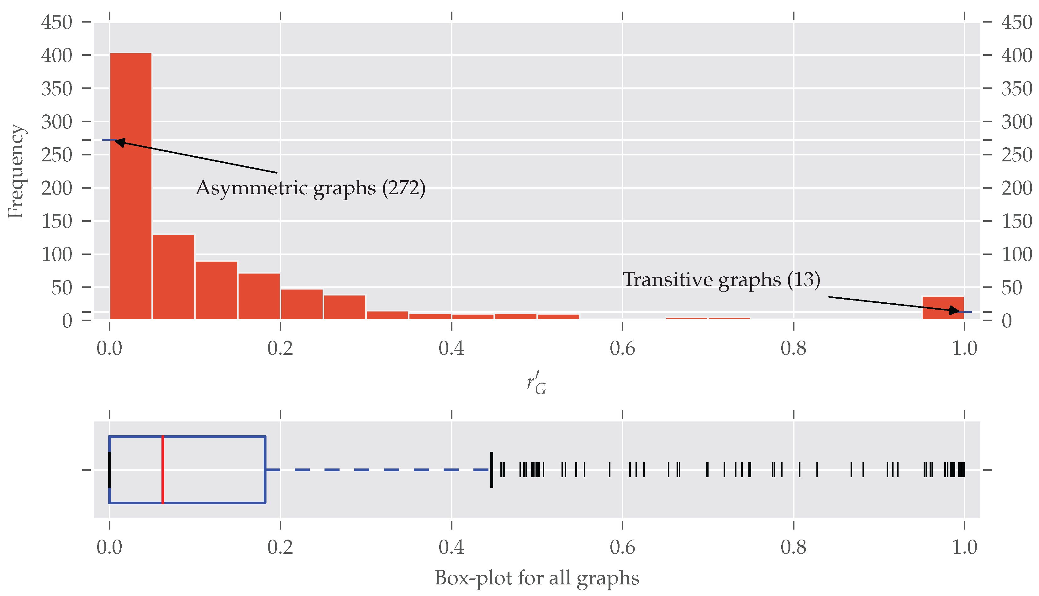
Until now we only distinguished between asymmetric and symmetric graphs without taking the degree of symmetry into account. In Figure 4 the histogram of the normalized redundancy is shown. One can see that most of the analyzed graphs have a relatively low normalized redundancy (over 80% of them with ). However, even a low redundancy of say 0.1 implies that about 10–20% of all nodes are affected by the symmetries, as the following example shows. is true for . If all nodes affected by are on exactly one orbit, approximately all orbits but one are trivial, which means about 10% of the nodes are affected. Conversely, about 20% of all nodes are affected if there are trivial and non-trivial orbits, each consisting of exactly two nodes. A further increase of non-trivial orbits is not possible (proof in Appendix B).
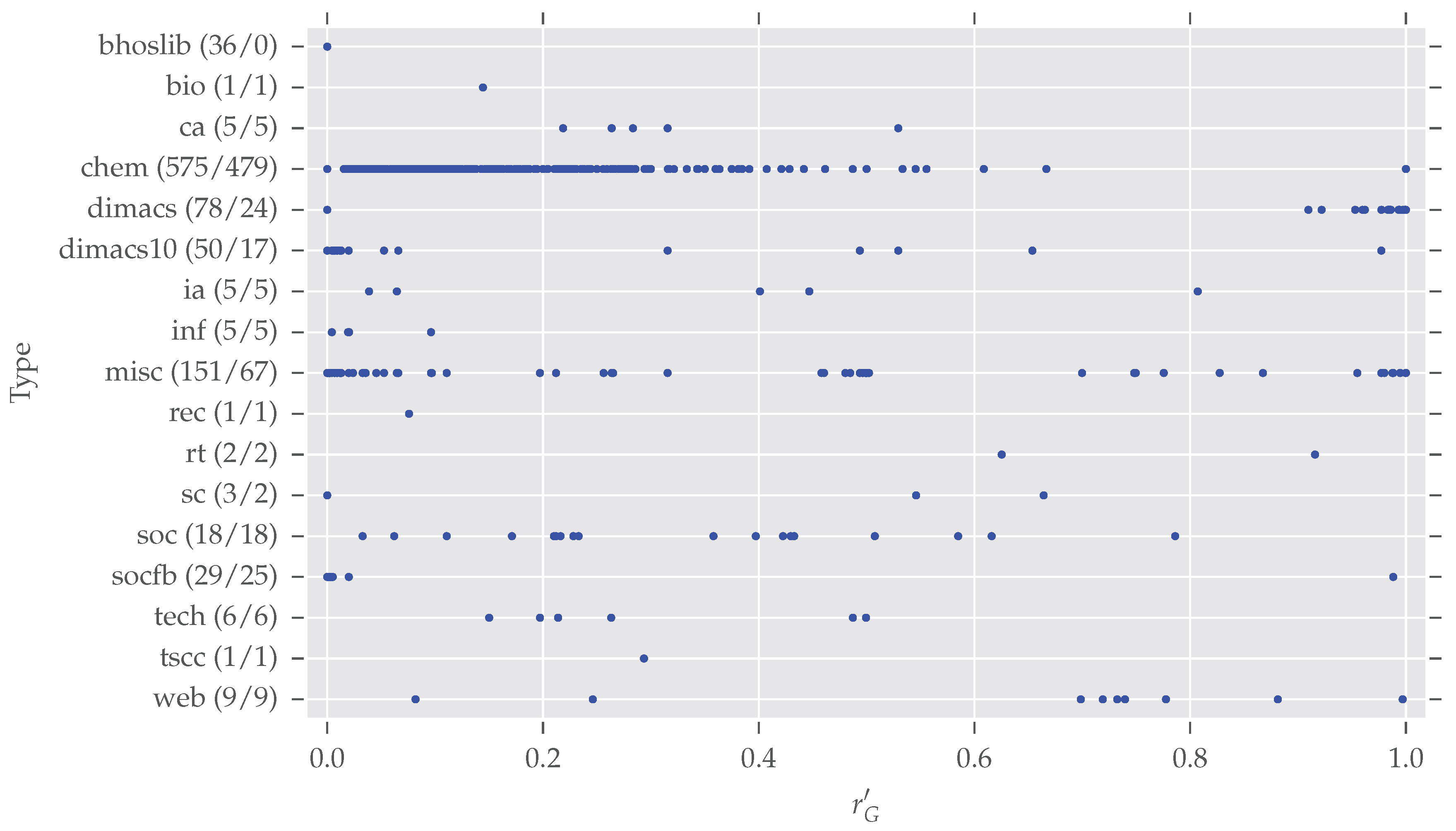
Due to the very diverse class sizes of the networkrepository.com data, we did not carry out an in-depth comparison of analysis results between different classes. Nonetheless, Figure 5 presents a glance at the distributions of normalized redundancy per class. In total, 975 graphs (duplicates among different classes are now included) are spread over 17 classes. Note that networkrepository.com has 21 different classes in total, due to the data selection described earlier, and some classes vanish in our analysis (“Brain Networks”, “Ecology Networks”, “Massive Network Data”, “Dynamic Networks”). However, we want to give some further information for the largest classes of our analysis.
- bhoslib (“Benchmarks with Hidden Optimum Solutions for Graph Problems”, http://www.nlsde.buaa.edu.cn/~kexu/benchmarks/graph-benchmarks.htm, last accessed 4 September 2017): All these graphs are asymmetric. They all are generated from the “Model RB” [33], a derived random graph model. As argued earlier, random graphs tend to be asymmetric.
- chem: This largest class contains cheminformatics data which has overall a large degree of symmetry. The origin of all those networks is described by Borgwardt et al. [34]: They extracted proteins from an online enzyme information system and transformed them into undirected graphs. The nodes are labeled and we also took this labeling into account (see our discussion on graph simplification in Section 3) by additionally providing the partition vector of labels to the saucy call. saucy supports initially labeled nodes as starting point for the search procedure.
- dimacs/dimacs10: These datasets come from different DIMACS challenges (http://dimacs.rutgers.edu/Challenges/, last accessed 4 September 2017). The former, especially, contains a large number of highly symmetric graphs, but also many asymmetric graphs as described above.
- misc: This class contains datasets which seem not to fit any of the other classes. Therefore it is hard to make any valid assertions. Certainly one can see some interesting patterns—many graphs exist with and there are five subclasses with —which gives room for further inspections.
- socfb: Although these networks seem to be mostly asymmetric, only four of the 29 actually are. All these graphs are quite large—more than 15,000 nodes on average—as they represent parts of the Facebook social network.
It is worth noting that the 11 remaining smaller classes contain nearly only symmetric networks (54 of 55 are symmetric). Overall, these quick inspections show there exist differences between the different classes.
5. Conclusions
This article makes the following contributions to the analysis of symmetry of graphs:
- It is the first large-scale study of symmetry of graphs (with about 900 graphs in the main part and with almost 800 simplified graphs in the appendix). Almost three quarters of the graphs are symmetric.
- The study shows that—except for the artificial random graphs (the class bhoslib)—all other classes of real-world networks contain a high number of graphs with symmetries.
- The analysis procedure is described in the appendix and its implementation is made available as Supplementary Materials.
- Last, but not least, for the purpose of summarizing the symmetry analysis of a large set of graphs, an improved measure of symmetry of a graph, namely a normalized version of the network redundancy measure, is derived. It has the intuitive property that completely asymmetric graphs have a measure of 0 and completely symmetric graphs a measure of 1. In contrast, the original definition by MacArthur et al. [19] yields different values for different asymmetric graphs, which makes them incomparable by the measure.
For graph clustering, the results of this study imply that an analysis of symmetry has the potential of considerably improving applied work in graph clustering and social-network analysis. The reason for this are two problems discussed in detail by Ball and Geyer-Schulz [4] (Section 3):
- Multiple equivalent solutions of graph clustering algorithms with unstable clusters.
- Diagnostic problems with all classic partition comparison measures. They fail to identify automorphic partitions as equivalent.
6. Outlook
This section is structured in a description of our current work in graph clustering diagnostics and some educated guesses on potential application fields. We consider the implementation of the graph-analysis procedure for this study as a stepping stone to the extraction of the generators of the automorphism group of a graph. However, given the automorphism group of a graph (or its generators), we currently work on the construction of invariant graph partition-comparison measures. Combined with the standard partition-comparison measures, one can separate stable and unstable areas of graphs and perform a detailed and quantified analysis of the effects of graph symmetries. An early example of this kind of analysis for the optimal solution of the famous Karate graph [29] can be found in [4] (pp. 18–19). For the Karate example, our analysis showed that symmetry did not affect the modularity optimal solution. In this example, the originally published solution is both optimal and stable and, in addition, easily interpretable by sociologists.
However, in general, this may not be the case, and without analysis, one does not know. In our own research, we focus on graph clustering, and checking the impact on modularity maximizing graph partitions shall be accomplished in our future research.
This article lays the foundation for further research in terms of possible influences on network analysis methods. Having shown that symmetries are very likely to exist in real-world networks, it is worth inspecting such methods and the outcome of them on how they are affected by graph symmetries. Also, the interpretation of the results must possibly be reconsidered. For example, what is the implication of two clusters of nodes (result of a graph clustering algorithm) where nodes can be exchanged between clusters by an automorphism (single nodes are all nodes at once)? Or, what does it mean if nodes inside a cluster can be mapped onto each other?
The comparison of the within-class distributions of the normalized network redundancy in Figure 5 shows that graphs from different classes have a different degree of symmetry. We have not performed an in-depth analysis of graphs aggregated by the different classes, but a glance on it showed that there is room for further research. Especially, the connection between other properties of graphs—like density or clustering coefficient [16]—and the observed symmetry could be of interest. If a high correlation of symmetry with other graph properties or measures exists, this could ease the decision of whether to perform a symmetry analysis if the considered property/measure is cheap to obtain.
Also, the connection between the graph’s underlying degree distribution—which is the base of most graph models, for example, [35]—and symmetry characteristics could help to better understand complex networks. This is because the degree distribution has a direct impact on the theoretically possible automorphisms, as only nodes having the same degree can be mapped onto each other.
A different area of application is in communication networks. One line of research in this area relates to information cascades in networks [36], which describe the spread of some information (or disease) between connected individuals. Again, one could ask what is the impact of redundant nodes? Do they speed up or slow down the spread of information? Another line of research deals with the optimal construction of technical communication networks with regard to their computational complexity, the number of components (gates), noise tolerance in communication channels, or deterministic error reduction in randomized polynomial time algorithms. The theoretical base of this is the construction of expander graphs by using the proved Ramanujan conjecture from the theory of automorphic forms, which is nicely summarized in [37], and a recent survey of applications in theoretical computer science is presented by Hoory et al. [38]. We conjecture that expander graphs could be a comparison standard for information cascades in complex real networks.
Supplementary Materials
The analysis scripts and analysis data are available online at https://github.com/FabianBall/networkrepository_analysis.
Acknowledgments
We acknowledge support by Deutsche Forschungsgemeinschaft and Open Access Publishing Fund of Karlsruhe Institute of Technology. Furthermore, we thank the reviewers for their helpful comments.
Author Contributions
Fabian Ball has implemented the whole analysis procedure and has written the paper. Andreas Geyer-Schulz provided substantial comments, hints, and corrections in form and content. Also did he come up with the idea of the expander graphs in the outlook.
Conflicts of Interest
The authors declare no conflict of interest.
Appendix A. Analysis Procedure Details
Here, further detail on the graph analysis presented is given in order to make the results reproducible. The complete analysis procedure is split into several Python (https://www.python.org/, last accessed 4 September 2017, release version 2.7.13 was used) scripts that are available as Supplementary Materials. Furthermore, intermediary results are also provided to allow reconstruction of our results.
Appendix A.1. Metadata Retrieval and Download Selection
As networkrepository.com contains not only small but also very large datasets (“Massive Network Data”) of several gigabytes, analyzing everything was not an option. Therefore, we retrieved the table that contains all datasets (http://networkrepository.com/networks.php, last accessed 4 September 2017) as a starting point. A script loads this table and downloads all datasets (the download link is part of the metadata) that are smaller than approximately 70 megabytes (desired minimum/maximum sizes are configurable).
A second script saves the data from the table of all networks to a comma-separated values (.csv) file. This information is later needed for the class-wise statistics.
Appendix A.2. Main Analysis
The core of the analysis is a script that iterates over all downloaded datasets, extracts them (they are provided as compressed archives), determines the graph data format (Matrix Market exchange or edge list), loads the data, filters the datasets to use (only simple and connected graphs), and eventually computes the desired information (modularity and normalized network redundancy) for each graph. From the graphs having the Matrix Market exchange format, only those were selected which had the following meta-information in the first line:
%%MatrixMarket matrix coordinate pattern symmetric
This corresponds to a symmetric matrix (adjacency matrices of graphs are always symmetric) with a coordinate format and pattern-encoded entries. That is, each line contains only the position of the entry in the matrix and no additional weight. For details on the format see Boisvert et al. [25]. To parse the Matrix Market format, the routines scipy.io.mminfo and scipy.io.mmread were used (http://scipy.org/scipylib/, last accessed 4 September 2017, release version 0.18.1 was used). scipy.io.mmread returns a matrix that can then be used as input parameter for a networkx.Graph (http://networkx.github.io/, last accessed 4 September 2017, release version 1.11 was used).
The edge list format was more problematic as no official documentation could be found. However, the format described by [26] (Chapter 9) matches the format (the files have a “.edges” extension). Unfortunately, the files with this edge list format did not always strictly follow the patterns. We only accepted datasets that
- had no header and a simple edge list (cf. the matrix position),
- had a header bip unweighted or bipartite unweighted and a simple edge list,
- had a header sym unweighted or symmetric unweighted or undirected unweighted and a simple edge list,
- had a header or not (according the rules above) and an edge list, where the third column’s values are timestamps, not weights.
The header is everything before the actual edge list. In addition, graphs that were denoted bip/bipartite had to be transformed, as the nodes from either node set were labeled and . After transformation, the nodes were labeled and .
Some datasets (actually, only the networks from the “chem” class) provided in the edge list format additionally include a second file with the extension “.nodes”. This file contains the node labels in the format node_id label. This information was turned into a vector of node labels and used as an additional parameter to call saucy.
Independently from the graph data format, we checked if the graphs were connected and that neither multiple edges nor loops exist. Everything described above was necessary to ensure we only analyze simple graphs as we have argued in Section 3. For the automorphism group analysis we used saucy (http://vlsicad.eecs.umich.edu/BK/SAUCY/, last accessed 21 November 2017, release version 3 was used), which was called through our own Python binding pysaucy (https://github.com/FabianBall/pysaucy, last accessed 22 December 2017, release version 0.3.1 was used). If a vector of node labels was available, this information was provided as an additional parameter for the saucy call. Modularity was the result of utilizing the RG graph clustering algorithm [27]. The call was also wrapped by our Python binding pycggcrg (https://github.com/FabianBall/pycggcrg, last accessed 22 December 2017, release version 0.2.3 was used). The results of the main step were again saved to a csv file.
Appendix A.3. Statistics
Prior to computing the statistics, which can be found in Section 4, manual postprocessing was done. This was important to exclude any duplicates from the analysis on the complete data that is not yet grouped by classes. To achieve this, we sorted the data—opening the results from the previous step with standard spreadsheet software—by n, m, and num_orbits. For the graphs that had the same values for these three characteristics, all the other information was compared—which had also to be the same or similar if the graphs were duplicates—and as a last check, the names were compared. If the names were obviously similar, a duplicate was found. For example, karate.mtx and soc-karate.mtx both are the Karate network [29].
In a last script, we combined the metadata (needed for class information) and the analysis data from the previous step to compute the final statistics.
Appendix B. Maximum Fraction of Affected Nodes for Fixed Normalized Redundancy
Theorem A1.
Given the normalized network redundancy (for ), approximately a fraction of λ to nodes are affected by .
Proof.
Let . can be written as where is the number of orbits of fixed nodes—the unaffected ones—and l is the number of non-trivial orbits. All nodes on non-trivial orbits are affected by . It follows that with , as at least one non-trivial orbit must exist if is not trivial. So for , about nodes are unaffected, thus nodes are affected by .
As n is fixed, k decreases with increasing l which means the number of affected nodes increases. Additionally, must hold with being the non-trivial orbits. Combining both requirements yields which can be simplified to . Maximizing the factor l is possible up to as any shorter orbit would be trivial. It follows , thus nodes are unaffected by and nodes are affected. ☐
Lemma A1.
If , possibly all nodes are affected by .
Proof.
This is a direct consequence of the proof of Theorem A1. ☐
Example A1.
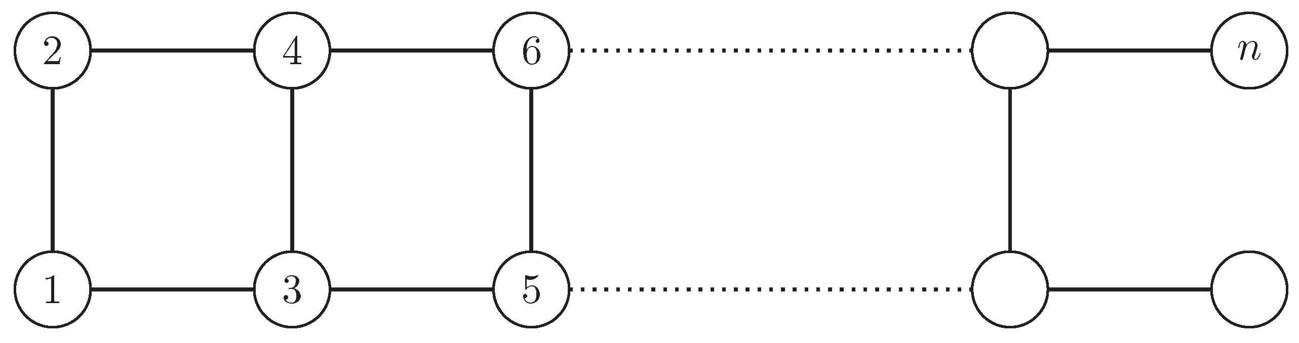
The graph in Figure A1 has although all its nodes are affected by . The orbit partition is which implies (for large n).
Figure A1.
A graph of an even number of nodes n for which the normalized network redundancy does not capture the high degree of symmetry, as no node is fixed by the automorphism group. The example shows that the (normalized) redundancy does not distinguish between the questions how many redundancies exist ( means 50% of the nodes have a redundant counterpart) and how robust is an existing redundancy ( means 50% are structurally identical, therefore redundant, and the other 50% are not redundant).

Appendix C. Additional Diagrams
Figure A2.
The histogram and box-plots for the number of nodes n. The x-axis and the bin widths follow a log-scale. Most graphs have between 10 and 100 nodes, and relatively fewer symmetries were found in medium-sized graphs, which coincides with the findings in Figure 2.
Figure A2.
The histogram and box-plots for the number of nodes n. The x-axis and the bin widths follow a log-scale. Most graphs have between 10 and 100 nodes, and relatively fewer symmetries were found in medium-sized graphs, which coincides with the findings in Figure 2.
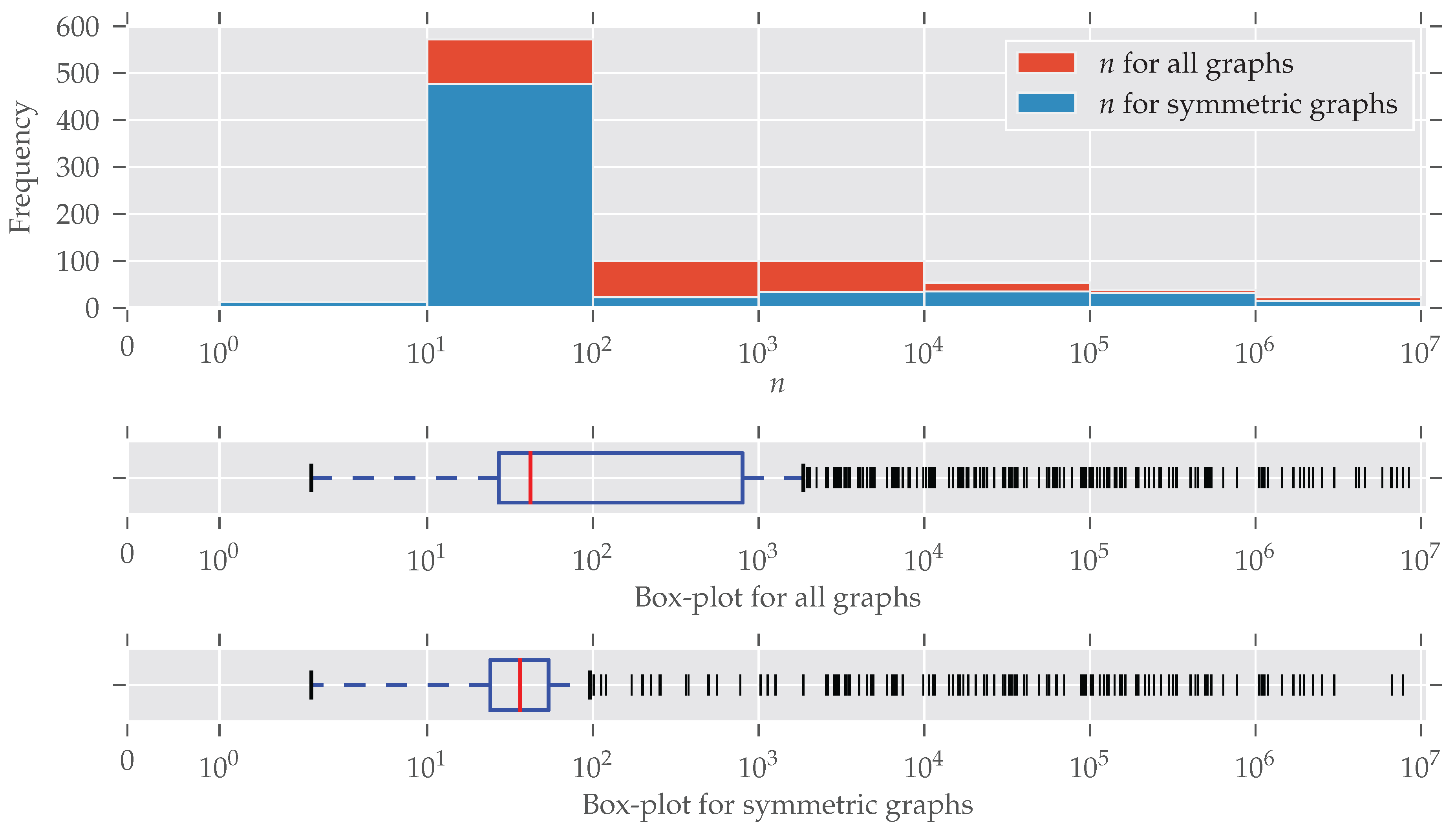
Figure A3.
The density of the graphs given their modularity Q. As stated in Section 4, modularity decreases with increasing density.
Figure A3.
The density of the graphs given their modularity Q. As stated in Section 4, modularity decreases with increasing density.
Appendix D. Results of Simplified Networks
As we have argued in Section 3.4, disconnected and non-simple graphs were not analyzed. However, we think it is a pity if only one third of the retrieved data sets is actually analyzed. Therefore, we decided to “simplify” the 1805 sorted-out graphs, remove duplicates, and also perform the analysis on them. From these datasets, 383 are disconnected and 420 are still invalid. The reason why they are invalid is that they have an asymmetric adjacency matrix and it is not clear from the data how to interpret it. One possibility is that they are bipartite graphs.
Due to the simplification (i.e., removing loops, edge weights, multiple edges), a large number of networks are duplicates, as often some datasets are only distinguished by having, for example, different edge weights. From the 1002 simplified and analyzed graphs, 797 unique datasets remained, and the results are shown in Table A1 and Figure A4. It can be seen that the simplified graphs are substantially larger than the ones analyzed in Section 3 and Section 4, are more modular, and have a higher degree of symmetry.
We leave further analysis of this data for future research and conclude that the underlying structure of the non-simple graphs has an even higher degree of symmetry, which emphasizes the message of this article.

Table A1.
Statistics for the simplified networkrepository.com datasets. 163 of the 797 graphs are asymmetric, therefore % of the graphs are symmetric. The row and column labels are the same as in Table 1.
Table A1.
Statistics for the simplified networkrepository.com datasets. 163 of the 797 graphs are asymmetric, therefore % of the graphs are symmetric. The row and column labels are the same as in Table 1.
| n | m | Q | |||
|---|---|---|---|---|---|
| count | 797 | 797 | 797 | 797 | 797 |
| mean | 70,041 | 7.0852 × 10 | 0.73453 | 0.4275 | 2.3286 × 10 |
| std | 2.9308 × 10 | 1.6665 × 10 | 0.20054 | 0.36822 | 6.5740 × 10 |
| min | 16 | 46 | 0 | 0 | 1 |
| 25% | 2534 | 11,173 | 0.65179 | 0.00412 | 2 |
| 50% | 10,605 | 89,927 | 0.79553 | 0.49254 | 3.3692 × 10 |
| 75% | 43,618 | 5.5493 × 10 | 0.87875 | 0.76424 | 2.9131 × 10 |
| max | 6.6865 × 10 | 1.7233 × 10 | 0.99771 | 1 | 1.8559 × 10 |
Figure A4.
The histogram and box-plots for the modularity Q as in Figure 3.
Figure A4.
The histogram and box-plots for the modularity Q as in Figure 3.

References
- Gross, D.J. The Role of Symmetry in Fundamental Physics. Proc. Natl. Acad. Sci. USA 1996, 93, 14256–14259. [Google Scholar] [CrossRef] [PubMed]
- Balaban, A.T. Applications of Graph Theory in Chemistry. J. Chem. Inf. Comput. Sci. 1985, 25, 334–343. [Google Scholar] [CrossRef]
- Dehmer, M.; Mowshowitz, A. A History of Graph Entropy Measures. Inf. Sci. 2011, 181, 57–78. [Google Scholar] [CrossRef]
- Ball, F.; Geyer-Schulz, A. Weak Invariants of Actions of the Automorphism Group of a Graph. Arch. Data Sci. Ser. A 2017, 2, 1–22. [Google Scholar]
- Read, R.C.; Corneil, D.G. The Graph Isomorphism Disease. J. Graph Theory 1977, 1, 339–363. [Google Scholar] [CrossRef]
- Lubiw, A. Some NP-Complete Problems Similar to Graph Isomorphism. SIAM J. Comput. 1981, 10, 11–21. [Google Scholar] [CrossRef]
- McKay, B.D. Practical Graph Isomorphism. Congr. Numerantium 1981, 30, 45–87. [Google Scholar] [CrossRef]
- McKay, B.D.; Piperno, A. Practical Graph Isomorphism, II. J. Symb. Comput. 2014, 60, 94–112. [Google Scholar] [CrossRef]
- Junttila, T.; Kaski, P. Engineering an Efficient Canonical Labeling Tool for Large and Sparse Graphs. In Proceedings of the 2007 Ninth Workshop on Algorithm Engineering and Experiments (ALENEX), New Orleans, LA, USA, 6 January 2007; pp. 135–149. [Google Scholar]
- Darga, P.T.; Sakallah, K.A.; Markov, I.L. Faster Symmetry Discovery Using Sparsity of Symmetries. In Proceedings of the 2008 45th ACM/IEEE Design Automation Conference, Anaheim, CA, USA, 8–13 June 2008; pp. 149–154. [Google Scholar]
- Babai, L. Graph Isomorphism in Quasipolynomial Time. arXiv, 2005; arXiv:1512.03547 [cs, math]. [Google Scholar]
- Babai, L. Graph Isomorphism in Quasipolynomial Time [Extended Abstract]. In Proceedings of the Forty-Eighth Annual ACM Symposium on Theory of Computing, Cambridge, MA, USA, 19–21 June 2016; ACM: New York, NY, USA, 2016; pp. 684–697. [Google Scholar]
- Garlaschelli, D.; Ruzzenenti, F.; Basosi, R. Complex Networks and Symmetry I: A Review. Symmetry 2010, 2, 1683–1709. [Google Scholar] [CrossRef]
- Erdős, P.; Rényi, A. Asymmetric Graphs. Acta Math. Hung. 1963, 14, 295–315. [Google Scholar] [CrossRef]
- Erdős, P.; Renyi, A. On Random Graphs I. Publ. Math. 1957, 6, 290–297. [Google Scholar]
- Newman, M.E. The Structure and Function of Complex Networks. SIAM Rev. 2003, 45, 167–256. [Google Scholar] [CrossRef]
- Xiao, Y.; MacArthur, B.D.; Wang, H.; Xiong, M.; Wang, W. Network Quotients: Structural Skeletons of Complex Systems. Phys. Rev. E 2008, 78, 046102. [Google Scholar] [CrossRef] [PubMed]
- Wang, H.; Yan, G.; Xiao, Y. Symmetry in World Trade Network. J. Syst. Sci. Complex. 2009, 22, 280–290. [Google Scholar] [CrossRef]
- MacArthur, B.D.; Sánchez-García, R.J.; Anderson, J.W. Symmetry in Complex Networks. Discret. Appl. Math. 2008, 156, 3525–3531. [Google Scholar] [CrossRef]
- Garrido, A. Symmetry in Complex Networks. Symmetry 2011, 3, 1–15. [Google Scholar] [CrossRef]
- Rossi, R.A.; Ahmed, N.K. The Network Data Repository with Interactive Graph Analytics and Visualization. In Proceedings of the Twenty-Ninth AAAI Conference on Artificial Intelligence, Austin, TX, USA, 25–30 January 2015; AAAI Press: Austin, TX, USA, 2015; pp. 4292–4293. [Google Scholar]
- Bastian, M.; Heymann, S.; Jacomy, M. Gephi: An Open Source Software for Exploring and Manipulating Networks. In Proceedings of the Third International AAAI Conference on Weblogs and Social Media, San Jose, CA, USA, 17–20 May 2009. [Google Scholar]
- Leskovec, J.; Krevl, A. SNAP Datasets: Stanford Large Network Dataset Collection; SNAP: Stanford, CA, USA, 2014. [Google Scholar]
- Bader, D.A.; Meyerhenke, H.; Sanders, P.; Schulz, C.; Kappes, A.; Wagner, D. Benchmarking for Graph Clustering and Partitioning. In Encyclopedia of Social Network Analysis and Mining; Springer: New York, NY, USA, 2014; pp. 73–82. [Google Scholar]
- Boisvert, R.F.; Pozo, R.; Remington, K.A. The Matrix Market Exchange Formats: Initial Design; Technical Report NISTIR 5935; National Institute of Standards and Technology, Applied and Computational Mathematics Division: Gaithersburg, MD, USA, 1996.
- Kunegis, J. Handbook of Network Analysis [KONECT—The Koblenz Network Collection]. arXiv, 2014; arXiv:1402.5500v3 [cs.SI]. [Google Scholar]
- Ovelgönne, M.; Geyer-Schulz, A.; Stein, M. Randomized Greedy Modularity Optimization for Group Detection in Huge Social Networks. In Proceedings of the 4th Workshop on Social Network Mining and Analysis, Washington, DC, USA, 25 July 2010; ACM: New York, NY, USA, 2010; pp. 1–9. [Google Scholar]
- Newman, M.E.J.; Girvan, M. Finding and Evaluating Community Structure in Networks. Phys. Rev. E 2004, 69, 026113. [Google Scholar] [CrossRef] [PubMed]
- Zachary, W.W. An Information Flow Model for Conflict and Fission in Small Groups. J. Anthropol. Res. 1977, 33, 452–473. [Google Scholar] [CrossRef]
- Fortunato, S.; Barthélemy, M. Resolution Limit in Community Detection. Proc. Natl. Acad. Sci. USA 2007, 104, 36–41. [Google Scholar] [CrossRef] [PubMed]
- Quintas, L.V. Extrema Concerning Asymmetric Graphs. J. Comb. Theory 1967, 3, 57–82. [Google Scholar] [CrossRef]
- Helmberg, C.; Rendl, F. A Spectral Bundle Method for Semidefinite Programming. SIAM J. Optim. 2000, 10, 673–696. [Google Scholar] [CrossRef]
- Xu, K.; Li, W. Many Hard Examples in Exact Phase Transitions. Theor. Comput. Sci. 2006, 355, 291–302. [Google Scholar] [CrossRef]
- Borgwardt, K.M.; Ong, C.S.; Schönauer, S.; Vishwanathan, S.V.N.; Smola, A.J.; Kriegel, H.P. Protein Function Prediction via Graph Kernels. Bioinformatics 2005, 21, i47–i56. [Google Scholar] [CrossRef] [PubMed]
- Albert, R.; Barabási, A.L. Statistical Mechanics of Complex Networks. Rev. Mod. Phys. 2002, 74, 47–97. [Google Scholar] [CrossRef]
- Jalili, M.; Perc, M. Information Cascades in Complex Networks. J. Complex Netw. 2017, 5, 665–693. [Google Scholar] [CrossRef]
- Lubotzky, A. Discrete Groups, Expanding Graphs and Invariant Measures; Birkhäuser Basel: Basel, Switzerland, 1994. [Google Scholar]
- Hoory, S.; Linial, N.; Wigderson, A. Expander Graphs and Their Applications. Bull. Am. Math. Soc. 2006, 43, 439–561. [Google Scholar] [CrossRef]
Figure 1.
Example of a two-step simplification of the graph (left) which is asymmetric. in the middle is still weighted but has a non-trivial automorphism group and G (right) is simple with a more complex automorphism group. Each automorphism group of the more complex graph(s) is a subgroup of the simpler graph(s): . This example shows how simplification of graphs by removing weights and/or loops can lead to additional symmetries. (a) The weighted graph which also has a loop at node 3. It has the trivial automorphism group ; (b) A simplified version of the graph with the following symmetries: ; (c) The simple graph G which has the automorphism group .
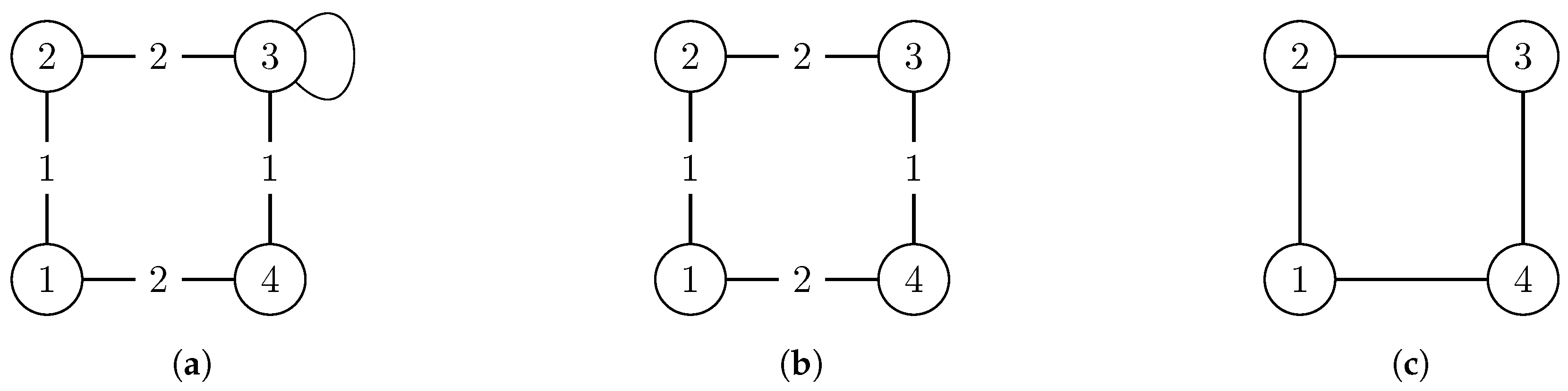
Figure 2.
The histogram and box-plots for the number of edges m. The x-axis and the bin widths follow a log-scale. In every bin, a substantial amount of graphs contain symmetries. An explanation of why the graphs with are relatively less-symmetric is given in the text. Nonetheless, symmetric graphs are present at all sizes.

Figure 3.
The histogram and box-plots for the modularity Q as a measure of cluster structure. All bins have an equal width of 0.05. Again, many graphs with partitions having a certain modularity value Q are found to be symmetric. Only graphs with a very low modularity seem to be substantially less symmetric, which is discussed in the text. There is no concise definition for which values of Q a partition of a graph is good, because this depends on the graph’s size. For smaller graphs, values greater than 0.3 are fine, for large graphs, values greater 0.9 are not unusual.

Figure 4.
The histogram and box-plot for the normalized redundancy for all 902 graphs. In total, there are 272 asymmetric and 13 completely symmetric (transitive) graphs. Most of the graphs have a quite low normalized redundancy, nevertheless about 70% of the analyzed data contain symmetries. The bin width is 0.05. The right skew of the distribution is underlined by the often-true relationship that the median (0.0625) is smaller than the mean (0.1514).

Figure 5.
The normalized redundancy distributions per class. The classes are (as named on networkrepository.com): bhoslib (“BHOSLIB”), bio (“Biological Networks”), ca (“Collaboration Networks”), chem (“Cheminformatics”), dimacs (“DIMACS”), dimacs10 (“DIMACS10”), ia (“Interaction Networks”), inf (“Infrastructure Networks”), misc (“Miscellaneous Networks”), rec (“Recommendation Networks”), rt (“Retweet Networks”), sc (“Scientific Computing”), soc (“Social Networks”), socfb (“Facebook Networks”), tech (“Technological Networks”), tscc (“Temporal Reachability Networks”), web (“Web Graphs”). After each class name, the tuple (“number of class members”, “number of symmetric class members”) is given. For this plot, duplicates from different classes were not removed to prevent a bias within classes. 975 networks are spread over the 17 classes. Details on the six largest classes are given in the text. The distributions of normalized redundancy per class differ strongly and with an exception of bhoslib, each class contains a large amount of symmetric graphs.

Table 1.
Statistics for the networkrepository.com datasets: Only 272 of the 902 graphs are asymmetric. count is the number of datasets on which the statistics per column were computed on, mean (std) is the respective mean value (standard deviation). min and max are the minimal/maximal values observed and the three remaining rows in between denote the two quartiles (25% and 75%) and the median (50%). The columns n (m) yield statistics on the number of nodes (edges) of the graphs, Q is the modularity, which measures (clustering) partition quality. The last two columns contain information on the symmetries, is the normalized redundancy (see Equation (2)) and the size of the automorphism group.
| n | m | Q | |||
|---|---|---|---|---|---|
| count | 902 | 902 | 902 | 902 | 902 |
| mean | 1.2796 × 10 | 4.1845 × 10 | 0.52569 | 0.1514 | 6.3659 × 10 |
| std | 8.6096 × 10 | 1.8654 × 10 | 0.24689 | 0.23447 | 1.9119 × 10 |
| min | 2 | 1 | 0 | 0 | 1 |
| 25% | 27 | 51 | 0.41563 | 0 | 1 |
| 50% | 42 | 84 | 0.57931 | 0.0625 | 4 |
| 75% | 800 | 24,489 | 0.66007 | 0.18182 | 24 |
| max | 1.1951 × 10 | 2.5166 × 10 | 0.99867 | 1 | 5.7420 × 10 |
© 2018 by the authors. Licensee MDPI, Basel, Switzerland. This article is an open access article distributed under the terms and conditions of the Creative Commons Attribution (CC BY) license (http://creativecommons.org/licenses/by/4.0/).
Share and Cite
MDPI and ACS Style
Ball, F.; Geyer-Schulz, A. How Symmetric Are Real-World Graphs? A Large-Scale Study. Symmetry 2018, 10, 29. https://doi.org/10.3390/sym10010029
AMA Style
Ball F, Geyer-Schulz A. How Symmetric Are Real-World Graphs? A Large-Scale Study. Symmetry. 2018; 10(1):29. https://doi.org/10.3390/sym10010029
Chicago/Turabian StyleBall, Fabian, and Andreas Geyer-Schulz. 2018. "How Symmetric Are Real-World Graphs? A Large-Scale Study" Symmetry 10, no. 1: 29. https://doi.org/10.3390/sym10010029
Note that from the first issue of 2016, this journal uses article numbers instead of page numbers. See further details here.