Accounting for Dissipation in the Scattering Approach to the Casimir Energy


1
Laboratoire Kastler Brossel (LKB), UPMC-Sorbonne Université, CNRS, ENS-PSL Research University, Collège de France, F-75252 Paris, France
2
Institut für Physik, Universität Augsburg, D-86135 Augsburg, Germany
*
Authors to whom correspondence should be addressed.
Symmetry 2018, 10(2), 37; https://doi.org/10.3390/sym10020037
Submission received: 22 December 2017
/
Revised: 19 January 2018
/
Accepted: 22 January 2018
/
Published: 26 January 2018
(This article belongs to the Special Issue Casimir Physics and Applications)
Abstract
:We take dissipation into account in the derivation of the Casimir energy formula between two objects placed in a surrounding medium. The dissipation channels are considered explicitly in order to take advantage of the unitarity of the full scattering processes. We demonstrate that the Casimir energy is given by a scattering formula expressed in terms of the scattering amplitudes coupling internal channels and taking dissipation into account implicitly. We prove that this formula is also valid when the surrounding medium is dissipative.
1. Introduction
Casimir physics has seen a renewed interest in recent decades thanks to new measurements of the Casimir interaction between macroscopic objects [1,2,3] with an improved precision [4,5,6,7,8], as well as efforts to meet the associated theoretical challenges [9,10,11,12,13,14]. In order to accurately reproduce the experimental data, a theoretical calculation has to model the optical properties of the materials used. A puzzling result of these comparisons is that some of the most precise experiments appear to agree well with the calculations only when the Ohmic losses in the metallic plates are neglected in the model. Several possible explanations of this puzzle have been discussed, but none of them seem to be satisfactory (a recent review is presented in [15]). For example, the electrostatic interaction between patches on the plates is certainly a possible systematic effect for Casimir force measurements [16,17,18,19], but it does not explain the discrepancy between theory and measurements [20,21].
This still-unsolved discrepancy between experiment and theory has led to discussions about the correctness of the theoretical formula used to describe Casimir interaction. In particular, it has been recently realized [22,23,24] that the calculations using the lossless plasma model were in fact neglecting the interaction between magnetically coupled induced currents due to a subtlety in the mathematical description of causality properties of the metallic optical response. Though it does not solve the discrepancy, this work has shed interesting new light on the derivation of the scattering formula used in most calculations. Among other worries, it has also been suggested that the scattering approach might not be valid for the dissipative metallic plates used in the experiments [25,26]. Some works have been devoted to ab initio treatments of the Casimir interaction between dissipative mirrors [27,28,29,30].
In the present article, we show that dissipation is taken into account in the usual scattering formula of the Casimir interaction energy [31,32]. We explicitly consider the channels responsible for dissipation in order to take advantage of the unitarity of the scattering processes. In the end, the Casimir energy is given by a scattering formula written in terms of the scattering amplitudes of the mirrors, implicitly accounting for the channels responsible for dissipation. In the context of Casimir physics, this result was already proven for the particular case of the plane-plane geometry [33,34], and the derivation in the present paper can be considered as a generalization to the case of an arbitrary geometry. In a broader context, it is reminiscent of properties known in the theory of resistance in mesoscopic physics [35], or that of quantum field propagation in a dissipative medium [36,37].
2. Scattering Interpretation of the Casimir Effect
Our starting point is the interpretation of the Casimir effect in terms of the scattering formula [31,32]. Since temperature does not play a key role in the considerations presented below, we assume for the sake of simplicity. We begin by considering a single object placed into a medium, with scattering of electromagnetic fluctuations by this object leading to a change of the vacuum energy written in terms of its scattering matrix
The change of vacuum energy is infinite when calculated for a single object, but its relevant part for estimating the Casimir effect turns out to be finite [38,39,40]. The phase shift is the trace of eigen-phase shifts summed over all scattering channels at a given frequency . The Formula (1) thus has a clear physical meaning when the scattering matrix is unitary, as it should if all scattering channels are taken into account. Accordingly, it is obvious that is real.
This discussion does not mean that (1) cannot be applied when dissipation enters the game. It only implies that all scattering channels responsible for dissipation processes must be included in the scattering theory. This can always be achieved, and necessarily leads to a unitary matrix. The general expression (1) always describes the modification of the vacuum energy due to the presence of scatterers. Another way to see that is to transform Equation (1) into an equivalent equation through an integration by parts and a rearrangement of terms:
Here, describes the vacuum energy of one mode at frequency , while is the modification of the density of states due to the presence of the scatterer [40,41]. Here again, this interpretation of (4) has a direct physical meaning when the scattering matrix is unitary.
In the following, we derive the expression for the Casimir interaction energy between two objects ① and ②. The set-up is displayed in Figure 1, with wavy lines representing dissipative channels for the objects and the medium. We apply the formula written above for the total scattering matrix S viewed as describing the change of the electromagnetic vacuum energy when two objects are placed in the surrounding medium at a distance L. As depicted in Figure 1, the total scattering matrix S can be decomposed into the scattering matrices and related to the individual objects, and the matrix describing the propagation between the two objects over a distance L through the medium. The expression for the Casimir interaction energy is then obtained as the change in the vacuum energy caused by the full scattering matrix S after extracting the part depending on the distance L.
We now introduce the notion of internal and external scattering channels. An internal scattering channel links the two objects. It represents, for example, an outgoing channel from object ① which becomes an incoming channel at object ② after propagation by a translation matrix, as discussed in Section 4. The channels which are not internal are named external channels. They account for the exchange of photons with the outside world and for quantum fluctuations from the environment. It is assumed that photons leaving through an external channel will not return coherently, but rather be absorbed in an excitation process in the outside world. Once these channels are included, the scattering matrices , , and are unitary, and therefore the total scattering matrix is unitary as well. The Casimir interaction is then given by the part of Equations (1) and (3), which depends on L. We show below that the Casimir energy can also be described by a simplified scattering formula written in terms of scattering amplitudes between internal channels only, with the channels responsible for dissipation taken into account implicitly [33,34].
3. Determinant Formula for Two Scatterers
In this section, we derive a relation involving determinants of scattering matrices for a scattering set-up with an internal structure described by two scattering matrices as depicted in Figure 2. In order to emphasize that the involved scattering matrices are general and not necessarily related to the scattering matrices introduced in Figure 1, we denote them by calligraphic symbols , , and . When applying the relation for the determinant (17) obtained at the end of this section, we will replace these general scattering matrices by specific scattering matrices related to the set-up shown in Figure 1.
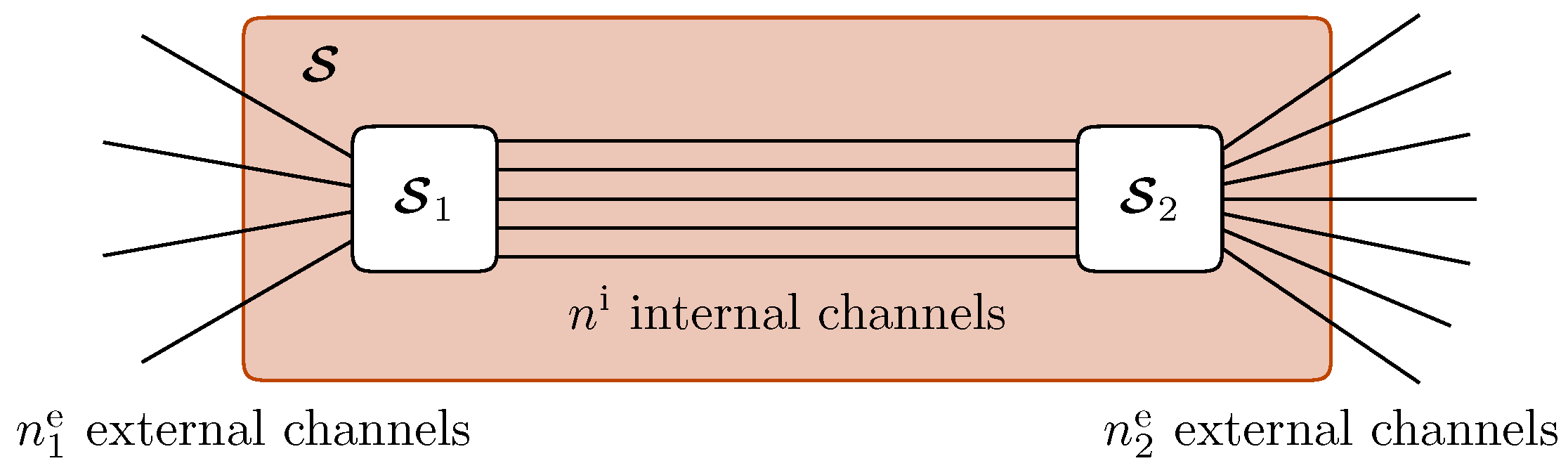
Ignoring the internal structure, the scattering properties can be described by a scattering matrix coupling the external channels among each other. Accounting for the internal structure, in addition to the and external channels associated with the scattering matrices and , respectively, one has internal channels coupling the two scatterers. Even though the two scatterers in Figure 2 are drawn at a certain distance, for the purpose of this section, we do not imply any effects of translation between the two scatterers. Such effects can be accounted for by an additional scattering matrix, as we will see in Section 4.
As the individual scattering matrices and couple internal (i) and external (e) channels among each other, we can express them in block matrix form as
The global scattering matrix is obtained by chaining the effect of the two individual scatterers
where the symbol ⋆ indicates that is not obtained by a simple matrix multiplication of and . In fact, the scattering matrices can be transformed into transfer matrices for which the chaining corresponds to a matrix multiplication [33]. From the resulting transfer matrix, one obtains the global scattering matrix, which can be expressed as a block matrix
where the blocks refer to the external channels associated with scatterers 1 and 2. Evaluating the chaining operation on and as just described, one finds
where
The matrices in (9) account for an arbitrary number of round trips along the internal channels between the two scatterers starting on scatterer 1 and scatterer 2, respectively, as can be seen by means of a Taylor expansion; e.g.,
The relations (8a) and (8c) are visualized in Figure 3, and the other relations are obtained by interchanging the two scatterers.
Relations (7)–(9) allow us to determine the determinant of the scattering matrix . In the derivation, we suppose that the three matrices , , and are unitary. From the property (A7) of the determinant of a unitary block matrix, we get together with the relations (8a) and (8d)
Then, we use a generalization of the matrix determinant lemma on the above expression (see the Appendix A). For instance, for the numerator we have according to (A5)
By applying (A7) to matrices and , we can express the determinants of the blocks and related to the external channels by those related to the internal channels, and , and obtain
where the last factor reads
This factor can be further evaluated by making use of (A8) yielding
4. Application to the Casimir Interaction Energy
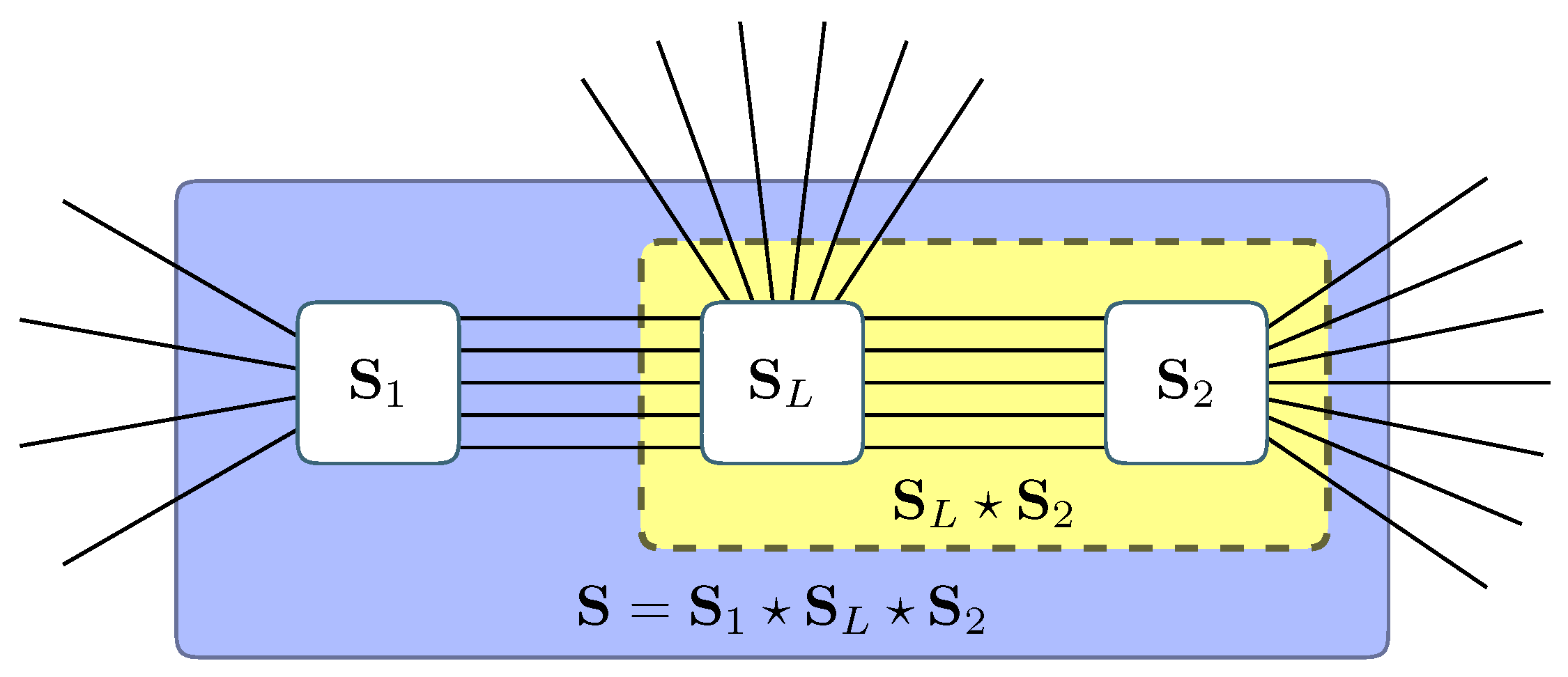
At first sight, it might appear that the result (17) can be directly applied to the expression for the Casimir energy (1) between two dissipative objects by replacing the general scattering matrices and in (17) by the scattering matrices and of the two dissipative objects. However, as already pointed out in the first paragraph of Section 3, the translation of the electromagnetic waves through a potentially dissipative medium between the two objects has not yet been accounted for. Actually, we have to consider the set-up depicted in Figure 4, where in addition to the scattering matrices and , a scattering matrix is present. This scattering matrix describes the translation of electromagnetic waves between the bases associated with objects ① and ② over a distance L. As shown in Figure 4, the operator involves a first set of internal channels connecting to , a second set of internal channels connecting to , and a set of external channels. The operator then has the same structure as in Equation (5). However, using the two sets of internal channels defined previously, the block itself has the following sub-structure:
Above, the vanishing blocks express the fact that no backscattering can occur during the propagation between the two objects. The blocks express the translation over a distance L from object ① to object ②, and vice-versa. Concrete examples will be discussed at the end of this section. Furthermore, couples to external channels describing the loss of photons and the influence of noise from the environment. Those losses are described by the blocks , and are directly responsible for the imaginary part of the intervening medium’s refractive index. The global scattering matrix associated with Figure 4 reads
In the chaining of scattering matrices, we are free to choose the order. As indicated by the box marked by a dashed line in Figure 4, we start by evaluating .
With and being unitary matrices, we can directly apply (17) by replacing and by and , respectively. However, reflecting the internal round-trips requires some attention. In contrast to Section 3, the internal channels between scattering matrices and are now interrupted by the scattering matrix , and we should consider as internal only those channels connecting and . In contrast, the channels connecting and are to be taken as external for the present consideration. Since does not induce backscattering, it follows that the purely internal part of vanishes, . As a consequence, is a unit matrix, reflecting the fact that no internal round trips are possible between and . From (17), we then obtain
Apart from , the matrix also contains the coupling between the internal channels due to reflection by the chain of scattering matrices . As explained before, does not by itself lead to a coupling of internal channels linked to object ①. This can happen only by means of sandwiched between translation matrices and through a dissipative medium over the distance L from object ① to object ② and back. In the last factor of (21), we thus have to set
We note that in the presence of a dissipative medium, and are non-unitary matrices.
We can now insert (21) together with (22) into (1) to obtain the change in the vacuum energy due to the dissipative scatterers separated by a dissipative medium. To obtain the Casimir interaction energy, we need to identify the part which depends on the distance L between the two objects. In (21), the first two factors depend only on properties of the individual objects, and are thus irrelevant for the Casimir interaction energy. Only the last two factors depend on L. However, the global scattering matrix contains a trivial dependence on L arising from the shift of the basis discussed before (19). This effect would survive even in the absence of the objects ① and ②, in which case the Casimir interaction energy vanishes. We are thus left with the last factor. In view of (1) and (2), we finally obtain for the Casimir interaction energy
This expression depends only on the parts of the scattering matrices pertaining to the internal channels. Nevertheless, the properties of these parts reflect the dissipative properties of the objects and the medium in between.
In the form (23), the expression for the Casimir interaction energy is quite general and basis-independent. The Dzyaloshinskii–Lifshitz–Pitaevskii formula [42] is recovered in the case of a plane-plane geometry. In this geometry, it makes sense to work in a basis of plane waves characterized by the quantum numbers , where is the transverse part of the wave vector with respect to the unit vector normal to the two planes (note that is a real quantity since Im[] is perpendicular to surfaces of constant amplitudes) and denotes the polarization. In this basis and this geometry, both the scattering matrix and the translation matrix are diagonal, with matrix elements given by the Fresnel reflection amplitude and , respectively. The lossy propagation is conveniently described by introducing a complex refractive index whose imaginary part is identified with the attenuation constant. In the case of anisotropic intervening media, the refractive index becomes a tensor instead of a scalar. Consequently, channels associated with different polarizations of the electromagnetic field can be coupled through the scattering and translation operators and .
Another useful basis is the multipole basis whenever the system under study has some degree of spherical symmetry. For a sphere, the scattering matrix is diagonal with elements determined by the Mie scattering amplitudes. The set of internal channels between a sphere and another object consists of an infinite number of multipoles arising from translation formulas between spherical waves (see, e.g., [43]), so that the translation matrix is not diagonal.
For geometries involving gratings (see, e.g., [44]), one works once again in a plane-wave basis. In this case, it is the scattering matrix which is not diagonal due to the non-specular nature of the reflection by a grating. Therefore, the plane-plane geometry is one of the few examples where both scattering and translation matrices are diagonal (the other one being the somewhat unrealistic geometry consisting of two concentric spheres). In general, at least one the two matrices is not diagonal. It is possible to treat in a similar way non-specular scattering for a Drude metal with Ohmic behaviour related to a disordered distribution of impurities [45]. Finally, we note that the formalism presented in this manuscript can be generalized so as to include off-the-energy-shell scattering matrix elements in order to describe the dynamical Casimir effect observed in recent experiments [46,47,48,49].
5. Conclusions
We have derived an expression for the Casimir interaction energy between dissipative objects embedded in a dissipative medium using the formalism of the scattering theory. The determinant of the total scattering matrix can be factored out into parts depending or not on the distance between the objects. The Casimir interaction energy is expressed using the distance-dependent part. Our final result (23) depends exclusively on scattering matrix elements involving internal channels. Dissipation thus appears only implicitly in the scattering amplitudes, as the blocks over the internal channels are non-unitary.
Author Contributions
All authors contributed equally.
Conflicts of Interest
The authors declare no conflict of interest.
Appendix A. Useful Lemmas
In this appendix, we gather several relations pertaining to block matrices which are required in the main part of the text. Let
be a block matrix. Its determinant can expressed either as
or
provided that the blocks and/or are invertible. The Schur complements of the blocks and in are defined as
respectively. From the two expressions (A2) and (A3) for the determinant of , one obtains the matrix determinant lemma
if the lower right block in is replaced by .
For the remainder of this section, we assume to be unitary. If both blocks and are invertible, the relation reads
From the upper-left block together with (A3), we find
Together with (A4b), the same relation yields
References
- Casimir, H.B.G. On the attraction between two perfectly conducting plates. Proc. K. Ned. Akad. Wet. 1948, 51, 793–796. [Google Scholar]
- Lifshitz, E.M. The theory of molecular attractive forces between solids. Sov. Phys. JETP 1956, 2, 73–83. [Google Scholar]
- Schwinger, J.; DeRaad, L.L.; Milton, K.A. Casimir effect in dielectrics. Ann. Phys. 1978, 115, 1–23. [Google Scholar] [CrossRef]
- Decca, R.S.; López, D.; Fischbach, E.; Klimchitskaya, G.L.; Krause, D.E.; Mostepanenko, V.M. Precise comparison of theory and new experiment for the Casimir force leads to stronger constraints on thermal quantum effects and long-range interactions. Ann. Phys. 2005, 318, 37–80. [Google Scholar] [CrossRef]
- Decca, R.S.; López, D.; Fischbach, E.; Klimchitskaya, G.L.; Krause, D.E.; Mostepanenko, V.M. Tests of new physics from precise measurements of the Casimir pressure between two gold-coated plates. Phys. Rev. D 2007, 75, 077101. [Google Scholar] [CrossRef] [Green Version]
- Masuda, M.; Sasaki, M. Limits on nonstandard forces in the submicrometer range. Phys. Rev. Lett. 2009, 102, 171101. [Google Scholar] [CrossRef] [PubMed]
- Sushkov, A.O.; Kim, W.J.; Dalvit, D.A.R.; Lamoreaux, S.K. New experimental limits on non-Newtonian forces in the micrometer range. Phys. Rev. Lett. 2011, 107, 171101. [Google Scholar] [CrossRef] [PubMed]
- Chang, C.-C.; Banishev, A.A.; Castillo-Garza, R.; Klimchitskaya, G.L.; Mostepanenko, V.M.; Mohideen, U. Gradient of the Casimir force between Au surfaces of a sphere and a plate measured using an atomic force microscope in a frequency-shift technique. Phys. Rev. B 2012, 85, 165443. [Google Scholar] [CrossRef]
- Lambrecht, A.; Reynaud, S. Casimir force between metallic mirrors. Eur. Phys. J. D 2000, 8, 309–318. [Google Scholar] [CrossRef]
- Boström, M.; Sernelius, B.E. Thermal effects on the Casimir force in the 0.1–5 μm range. Phys. Rev. Lett. 2000, 84, 4757–4760. [Google Scholar] [CrossRef] [PubMed]
- Milton, K.A. Recent developments in the Casimir effect. J. Phys. Conf. Ser. 2009, 161, 012001. [Google Scholar] [CrossRef]
- Rahi, S.J.; Emig, T.; Graham, N.; Jaffe, R.L.; Kardar, M. Scattering theory approach to electrodynamic Casimir forces. Phys. Rev. D 2009, 80, 085021. [Google Scholar] [CrossRef]
- Klimchitskaya, G.L.; Mohideen, U.; Mostepanenko, V.M. The Casimir force between real materials: Experiment and theory. Rev. Mod. Phys. 2009, 81, 1827–1885. [Google Scholar] [CrossRef]
- Ingold, G.-L.; Lambrecht, A.; Reynaud, S. Quantum dissipative Brownian motion and the Casimir effect. Phys. Rev. E 2009, 80, 041113. [Google Scholar] [CrossRef] [PubMed]
- Reynaud, S.; Lambrecht, A. Casimir Forces and Vacuum Energy. In Quantum Optics and Nanophotonics; Lecture Notes of the Les Houches Summer School 101; Fabre, C., Sandoghdar, V., Treps, N., Cugliandolo, L.F., Eds.; Oxford University Press: Oxford, UK, 2017; pp. 407–455. [Google Scholar] [CrossRef]
- Naji, A.; Dean, D.S.; Sarabadani, J.; Horgan, R.R.; Podgornik, R. Fluctuation-induced interaction between randomly charged dielectrics. Phys. Rev. Lett. 2010, 104, 060601. [Google Scholar] [CrossRef] [PubMed]
- Speake, C.C.; Trenkel, C. Forces between conducting surfaces due to spatial variations of surface potential. Phys. Rev. Lett. 2003, 90, 160403. [Google Scholar] [CrossRef] [PubMed]
- Kim, W.J.; Sushkov, A.O.; Dalvit, D.A.R.; Lamoreaux, S.K. Surface contact potential patches and Casimir force measurements. Phys. Rev. A 2010, 81, 022505. [Google Scholar] [CrossRef]
- Behunin, R.O.; Intravaia, F.; Dalvit, D.A.R.; Maia Neto, P.A.; Reynaud, S. Modeling electrostatic patch effects in Casimir force measurements. Phys. Rev. A 2012, 85, 012504. [Google Scholar] [CrossRef]
- Behunin, R.O.; Zeng, Y.; Dalvit, D.A.R.; Reynaud, S. Electrostatic patch effects in Casimir-force experiments performed in the sphere-plane geometry. Phys. Rev. A 2012, 86, 052509. [Google Scholar] [CrossRef]
- Behunin, R.O.; Dalvit, D.A.R.; Decca, R.S.; Genet, C.; Jung, I.W.; Lambrecht, A.; Liscio, A.; López, D.; Reynaud, S.; Schnoering, G.; et al. Kelvin probe force microscopy of metallic surfaces used in Casimir force measurements. Phys. Rev. A 2014, 90, 062115. [Google Scholar] [CrossRef]
- Intravaia, F.; Henkel, C. Casimir interaction from magnetically coupled eddy currents. Phys. Rev. Lett. 2009, 103, 130405. [Google Scholar] [CrossRef] [PubMed]
- Guérout, R.; Lambrecht, A.; Milton, K.A.; Reynaud, S. Derivation of the Lifshitz-Matsubara sum formula for the Casimir pressure between metallic plane mirrors. Phys. Rev. E 2014, 90, 042125. [Google Scholar] [CrossRef] [PubMed]
- Guérout, R.; Lambrecht, A.; Milton, K.A.; Reynaud, S. Lifshitz-Matsubara sum formula for the Casimir pressure between magnetic metallic mirrors. Phys. Rev. E 2016, 93, 022108. [Google Scholar] [CrossRef] [PubMed]
- Barash, Y.S.; Ginzburg, V.L. Electromagnetic fluctuations in matter and molecular (van der Waals) forces between them. Sov. Phys. Usp. 1975, 18, 305–322. [Google Scholar] [CrossRef]
- Bordag, M. Drude model and Lifshitz formula. Eur. Phys. J. C 2011, 71, 1788. [Google Scholar] [CrossRef]
- Jancovici, B.; Šamaj, L. Casimir force between two ideal-conductor walls revisited. Europhys. Lett. 2005, 72, 35–41. [Google Scholar] [CrossRef]
- Buenzli, P.R.; Martin, P.A. The Casimir force at high temperature. Europhys. Lett. 2005, 72, 42–48. [Google Scholar] [CrossRef]
- Intravaia, F.; Behunin, R. Casimir effect as a sum over modes in dissipative systems. Phys. Rev. A 2012, 86, 062517. [Google Scholar] [CrossRef]
- Bordag, M. Casimir and Casimir-Polder forces with dissipation from first principles. Phys. Rev. A 2017, 96, 062504. [Google Scholar] [CrossRef]
- Jaekel, M.T.; Reynaud, S. Casimir force between partially transmitting mirrors. J. Phys. I France 1991, 1, 1395–1409. [Google Scholar] [CrossRef]
- Ingold, G.-L.; Lambrecht, A. Casimir effect from a scattering approach. Am. J. Phys. 2015, 83, 156–162. [Google Scholar] [CrossRef]
- Genet, C.; Lambrecht, A.; Reynaud, S. Casimir force and the quantum theory of lossy optical cavities. Phys. Rev. A 2003, 67, 043811. [Google Scholar] [CrossRef]
- Lambrecht, A.; Maia Neto, P.A.; Reynaud, S. The Casimir effect within scattering theory. New J. Phys. 2006, 8, 243. [Google Scholar] [CrossRef]
- Engquist, H.L.; Anderson, P.W. Definition and measurement of the electrical and thermal resistances. Phys. Rev. B 1981, 24, 1151–1154. [Google Scholar] [CrossRef]
- Huttner, B.; Barnett, S.M. Quantization of the electromagnetic-field in dielectrics. Phys. Rev. A 1992, 46, 4306–4322. [Google Scholar] [CrossRef] [PubMed]
- Matloob, R.; Loudon, R.; Barnett, S.M.; Jeffers, J. Electromagnetic field quantization in absorbing dielectrics. Phys. Rev. A 1995, 52, 4823–4838. [Google Scholar] [CrossRef] [PubMed]
- Schwinger, J. The theory of quantized fields. VI. Phys. Rev. 1954, 94, 1362–1384. [Google Scholar] [CrossRef]
- Balian, R.; Duplantier, B. Electromagnetic waves near perfect conductors. I. Multiple scattering expansions. Distribution of modes. Ann. Phys. 1977, 104, 300–335. [Google Scholar] [CrossRef]
- Plunien, G.; Müller, B.; Greiner, W. The Casimir effect. Phys. Rep. 1986, 134, 87–193. [Google Scholar] [CrossRef]
- Souma, S.; Suzuki, A. Local density of states and scattering matrix in quasi-one-dimensional systems. Phys. Rev. B 2002, 65, 115307. [Google Scholar] [CrossRef]
- Dzyaloshinskii, I.E.; Lifshitz, E.M.; Pitaevskii, L.P. General theory of van der Waals’ forces. Sov. Phys. Usp. 1961, 4, 153–176. [Google Scholar] [CrossRef]
- Wittmann, R.C. Spherical wave operators and the translation formulas. IEEE Trans. Antennas Propag. 1988, 36, 1078–1087. [Google Scholar] [CrossRef]
- Guérout, R.; Lussange, J.; Chan, H.B.; Lambrecht, A.; Reynaud, S. Thermal Casimir force between nanostructured surfaces. Phys. Rev. A 2013, 87, 052514. [Google Scholar] [CrossRef]
- Cherroret, N.; Crépin, P.-P.; Guérout, R.; Lambrecht, A. Casimir-Polder force fluctuations as spatial probes of dissipation in metals. EPL 2017, 117, 63001. [Google Scholar] [CrossRef]
- Lambrecht, A.; Jaekel, M.-T.; Reynaud, S. Motion induced radiation from a vibrating cavity. Phys. Rev. Lett. 1996, 77, 615–618. [Google Scholar] [CrossRef] [PubMed]
- Maghrebi, M.F.; Golestanian, R.; Kardar, M. Scattering approach to the dynamical Casimir effect. Phys. Rev. D 2013, 87, 025016. [Google Scholar] [CrossRef]
- Wilson, C.M.; Johansson, G.; Pourkabirian, A.; Simoen, M.; Johansson, J.R.; Duty, T.; Nori, F.; Delsing, P. Observation of the dynamical Casimir effect in a superconducting circuit. Nature 2011, 479, 376–379. [Google Scholar] [CrossRef] [PubMed]
- Felicetti, S.; Sanz, M.; Lamata, L.; Romero, G.; Johansson, G.; Delsing, P.; Solano, E. Dynamical Casimir effect entangles artificial atoms. Phys. Rev. Lett. 2014, 113, 093602. [Google Scholar] [CrossRef] [PubMed]
Figure 1.
The Casimir interaction between two objects ① and ② at a distance L is considered. As indicated by the wavy lines, both objects as well as the medium in between are generally dissipative. The two objects are described by unitary scattering matrices and , which also account for the external channels associated with the dissipation. The unitary scattering matrix describes the translation between the reference frames of objects ① and ②, and also accounts for the external channels.
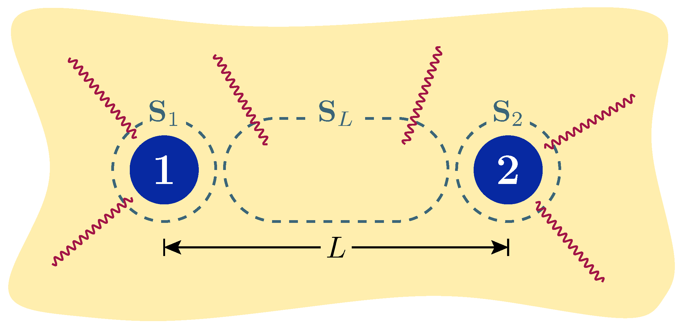
Figure 2.
Scattering geometry with internal structure. Seen from the outside, a total of external channels are coupled by a scattering matrix . The internal structure is accounted for by two scattering matrices and coupling internal channels to and external channels, respectively.
Figure 2.
Scattering geometry with internal structure. Seen from the outside, a total of external channels are coupled by a scattering matrix . The internal structure is accounted for by two scattering matrices and coupling internal channels to and external channels, respectively.

Figure 3.
Schematic representation of the blocks (a) and (b) of the total scattering matrix . The diagrams visualize the Equations (8a) and (8c), respectively. The two other blocks defined in (8b) and (8d) are obtained by exchanging the two objects.
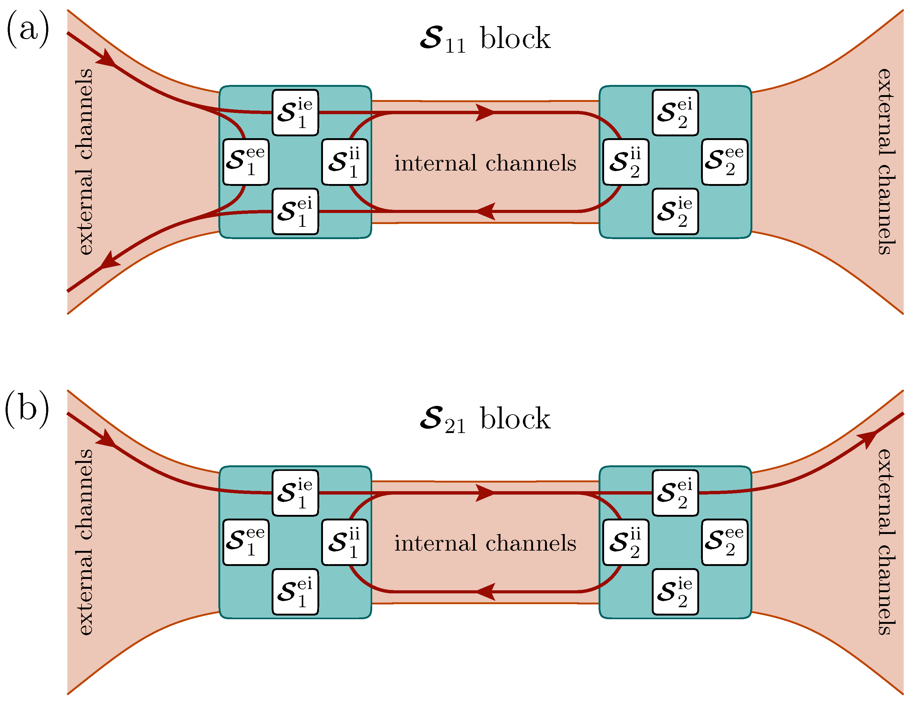
Figure 4.
Set-up required to describe the Casimir effect. Apart from the scattering matrices and , a scattering matrix describing the translation over a distance L is needed. In addition to the internal channels, all scattering matrices also couple to external channels, thus allowing the dissipation of the objects and the medium in between to be accounted for. In a first step, the combination indicated by the dashed box is considered.

© 2018 by the authors. Licensee MDPI, Basel, Switzerland. This article is an open access article distributed under the terms and conditions of the Creative Commons Attribution (CC BY) license (http://creativecommons.org/licenses/by/4.0/).
Share and Cite
MDPI and ACS Style
Guérout, R.; Ingold, G.-L.; Lambrecht, A.; Reynaud, S. Accounting for Dissipation in the Scattering Approach to the Casimir Energy. Symmetry 2018, 10, 37. https://doi.org/10.3390/sym10020037
AMA Style
Guérout R, Ingold G-L, Lambrecht A, Reynaud S. Accounting for Dissipation in the Scattering Approach to the Casimir Energy. Symmetry. 2018; 10(2):37. https://doi.org/10.3390/sym10020037
Chicago/Turabian StyleGuérout, Romain, Gert-Ludwig Ingold, Astrid Lambrecht, and Serge Reynaud. 2018. "Accounting for Dissipation in the Scattering Approach to the Casimir Energy" Symmetry 10, no. 2: 37. https://doi.org/10.3390/sym10020037
Note that from the first issue of 2016, this journal uses article numbers instead of page numbers. See further details here.