Lorentz Transformation, Poincaré Vectors and Poincaré Sphere in Various Branches of Physics

1
Faculty of Physics, University of Bucharest, P.O. Box MG-11, Bucharest Magurele 077125, Romania
2
Academy of Romanian Scientists, SplaiulIndependenţei 54, Bucharest 050094, Romania
Symmetry 2018, 10(3), 52; https://doi.org/10.3390/sym10030052
Submission received: 21 December 2017
/
Revised: 16 February 2018
/
Accepted: 18 February 2018
/
Published: 26 February 2018
(This article belongs to the Special Issue Modern Trends of Lorentz Symmetry and Lorentz Violation)
Abstract
:In the frame of a generic language extended from the polarization theory—comprising the notions of Poincaré vectors, Poincaré sphere, and P-spheres—a geometric approach to Lorentz transformations alternative to the Minkowskian one is given. Unlike the four-dimensional Minkowskian approach, this new approach operates in the three-dimensional space of Poincaré vectors.
1. Introduction
Nowadays, it is a well-known fact that Lorentz transformations, whose theory was deeply developed in special relativity (SR), constitute in fact the common underlying mathematics in specific problems of various fields of physics: polarization optics, multilayers, interferometry, laser cavity optics, geometrical optics, quantum optics, etc.
It was in 1963 that Richard Barakat [1] noticed first this fact, namely in the field of polarization theory (PT): one of the invariants of the coherency (polarization) matrix [2,3,4,5,6], its determinant, “has the form of a Lorentz line element. This fact allows us to apply group-theoretic methods employing the Lorentz group to discuss the coherency matrix. It seems surprising that no one called attention to this point”. Barakat came back to this issue only after two decades [7], but meantime Hiroshi Takenaka [8] has treated the action of deterministic polarization devices [2,3,4,5,6] on polarized light as a Lorentz transformation, in the frame of group theory. Since then a large amount of papers [9,10,11,12,13,14,15,16,17] has reinforced the Lorentzian approach in polarization theory.
In 1992, J. M. Vigoureux [18] noticed a similar situation in the theory of stratified planar structures (multilayers, ML): “the overall reflection coefficient of any number of isotropic media can be written directly by using a complex generalization of the relativistic composition law of velocities”. Again, a large amount of papers (e.g., [19,20,21,22,23,24] and references herein) has firmly introduced the Lorentzian approach in the field of multilayers, generally in terms of group theory. It is also Vigoureux who has drawn the important conclusion: “The composition law of velocities, which is usually presented as a specific property of relativity, appears here as a particular application to dynamics of a more general and more natural addition law in physics”. “The Einstein composition law [of velocities] appears to be a natural «addition» law of physical quantities in a closed interval” [18].
Similarly, the Lorentzian underlying mathematics structure of various problems was recognized in other fields of physics and these problems were treated in terms of Lorentz group or of various subgroups of Lorentz group: interferometry, geometrical optics, laser cavity optics, quantum optics, etc. ([25,26,27,28] and included references).
Finally, Abraham Ungar [29] has coined the term “gyrovectors” for the three-dimensional vectors whose modulus is limited to some constant value:
which “add” accordingly to what is known as the law of composition of relativistic allowed velocities [30]:
where we have labeled by v the velocity of a moving point M in an inertial reference system (IRS) , by u the velocity of the IRS with respect to the IRS , and by w the velocity of the moving point M as it is seen by an observer in ; u is the modulus of velocity u, which determines the strength of the boost. Here, the velocities are scaled at c (i.e., c is taken 1 by choosing conveniently the length or time unit [31]). The vectors (Equation (1)) with the composition law in Equation (2), have a “group-like” structure in the sense that this composition law ensures the closure condition (Equation (1)), but it is neither commutative nor associative.
Until now, a unilateral transfer of terms, ideas, and mathematical tools took place from theory of relativity to the above mentioned various domains of physics where Lorentz transformations work.
Recently, it was established that the law of composition of Poincaré vectors in polarization theory is identical with that of relativistic allowed velocities [32]. On the other hand, in the last decade, in polarization theory was extensively developed a geometrical algebraic technique, namely of the so called P-surfaces [3,33,34,35,36,37,38]. This approach can be exported in all of the problems whose underground is the Lorentz transformation.
In this paper, in the frame of a generic language extended from the polarization theory, we shall give a 3D geometric approach to Lorentz transformations, alternative to the four-dimensional Minkowskian one. The structure of the paper is the following:
In Section 2, by generalizing the notions of Poincaré vectors, Poincaré sphere, and P-spheres, specific to the polarization theory, a language that is applicable in all of the physical problems whose mathematical basis are Lorentz transformations is established.
In these terms, in Section 3, the mathematics of mapping the inner Poincaré spheres (P-spheres) in P-ellipsoids, by Lorentz boosts of any physical nature, is built up.
In Section 4, we shall illustrate this mapping for various values of the basic parameters of the problem, namely the radius of the P-sphere and the strength of the boost.
In Section 5, the characteristics of the resulted P-ellipsoids as functions of these parameters are analyzed. We will show that they become strongly non-linear, and, at the very end, indefinite functions in what in SR is the ultrarelativistic regime. This is a direct consequence of the fundamental constraint Equation (1), imposed in relativity by the second postulate, in polarization theory by the condition of non-overpolarizability, in the theory of multilayers by the condition of non-overreflectivity, etc.
The principal aim of the paper is to create a conceptual frame in which the Poincaré sphere geometric approach with its up-to-date ingredients should be implemented in all of the fields and problems where Lorentz transformation works, and to bring this approach up to the deepest conclusions. Subsidiarily, in the paper can be detected a second line: how this language and this approach, elaborated in polarization theory, are transferred in the main field dominated by the Lorentz transformation—the theory of relativity.
2. Poincaré Vectors, Poincaré Sphere and P-Spheres
2.1. Poincaré Vectors
Recently it was established [32] that in the action of an orthogonal dichroic device [4] on partially polarized light [2,3,4,5]—which, from a mathematical point of view, is a Lorentz boost—the Poincaré vectors, i.e., the normalized 3D vectorial part of the Stokes quadrivectors, , of the states of polarized light (SOPs) and of the polarization devices composes according to Equation (1):
or:
where:
- -
- are the Poincaré vectors of the incident light, dichroic device, and output light, respectively,
- -
- —the corresponding unit vectors,
- -
- —the degrees of polarization of the incident and emergent light, the degree of dichroism [39] of the dichroic device (the strength of the boost), and:
In a geometric image, the Poincaré vectors are 3D vectors confined in (“prisoners of”) a sphere of radius 1. In PT this sphere is the well-known Poincaré unit sphere. The constraint Equations (1) and (4) in PT is imposed by the fact that the degree of polarization cannot overpass the value 1 (the so-called “non-overpolarizability condition”). By consequence, the Poincaré polarization vectors cannot protrude the Poincaré sphere (here and in the following the lower index stands for the dimension of the space, e.g., 2 for the Poincaré sphere, 3 for the Poincaré ball, whereas the upper index stands for the radius of the sphere or of the ball).
Having in mind the state of arts presented in Introduction, we can realize now that in all of the physical problems whose underlying algebra is the Lorentz transformation, from various physical reasons (the second postulate in SR; the limited value, at 1, of the degree of polarization in PT and of the reflection coefficient in ML, etc.), the relevant vectors are under the constraint of Equation (1). We shall call them Poincaré vectors, irrespective of the physical field in which they appear.
2.2. Poincaré Sphere
This geometric tool, the Poincaré sphere, elaborated in the field of light polarization, can be extended to all of the physical phenomena with an underlying Lorentz symmetry. For example, the relativistic allowed velocities in SR are all enclosed in a sphere of radius c, which can be reduced to the unit sphere by a convenient choice of the unity of time or of that of length, which makes (the “normalized units”) [31]. This sphere is nothing else than the Poincaré unit sphere (in this case for relativistic allowed velocities).
It is worthwhile to remark that Poincaré has not connected his greatest intuition in PT—the Poincaré sphere [40]—with his fundamental intuitions in SR, what is understandable for the early days of both SR and PT. But, moreover, the Poincaré sphere, which was developed as a rigorous and powerful geometric tool in PT, was never transferred in SR (probably because of the preeminence and of the mathematical challenges of the Minkowskian geometric 3 + 1 representation in this field).
Until now, the transfer of ideas, language, mathematical tools, and results took place mainly from SR toward PT, ML, and the other fields mentioned above, whose Lorentzian underpinning was recognized, and in the benefit of these last fields. This is natural, because the theory of Lorentz transformations and of their representations was developed for more than 70 years exclusively in the frame of SR or in straight connection with it. But this geometrical tool, developed parallely in polarization theory, the Poincaré sphere—we understand now—can serve also the Lorentz transformations in any domain of physics. Recently, as we shall see in the next subsection, this tool was much refined. Its transfer from PT to SR and to all of the other fields mentioned above is now useful, now becomes actual.
2.3. P-Spheres
In the last decades in PT was elaborated a new approach to the problem of interaction between polarization devices and polarized light, the so-called method of degree of polarization (DoP) surfaces, or, synonymously, P-surfaces [3,33,34,35,36,37,38]. This is a global, holistic, mathematical technique developed in the frame of Poincaré geometric representation of SOPs: one analyses how a whole sphere of SOPs, , having the same degree of polarization, , is transformed by the action of a polarization device. Such a sphere was called in PT a DoP sphere, or a P-sphere. I shall adopt in the following the more recent term P-sphere, as imposed by the prestigious monograph [3], instead of the earlier one, DoP sphere; it is more suitable for the generic language I will propose here. In this language, the term P-sphere will be used with the signification of “inner Poincaré sphere”, a sphere of radius that is smaller than one.
Transposed in SR, the essence of this method is the following: Due to the second postulate of SR, all the relativistic allowed velocities are confined in a sphere of radius c (1 in the “natural system of units”), (Equation (1)). This is the Poincaré sphere of relativistic allowed velocities. Under the action of a Lorentz boost, any velocity sphere of radius v, , (i.e., any SR P-sphere, in the generic language) is deformed, because it is forced to remain enclosed in the Poincaré sphere (), irrespective how close are v and u (the boost velocity) to the velocity of light in vacuum. The behavior of the resulted velocity surface in function of the parameters v and u presents some strange aspects that reflect the counterintuitivity of the second postulate.
We will illustrate this behavior using the terms introduced above—Poincaré sphere, Poincaré vectors, P-spheres—in such a way that this language and approach should be applied word by word in all of the other fields and problems whose Lorentzian mathematical ground was or will be recognized.
3. Mapping of the P-Spheres by Lorentz Boosts: P-Ellipsoids
Let us start with the most expressive and compact form of the equation of composition of Poincaré vectors [30]:
I shall preserve here for the Poincaré vectors the labeling of Equation (2), rather than that of Equation (4), because it is familiar in SR, and by consequence, more widespread. This way, it will be easy, for fixing the ideas, to transpose the results obtained below in the particular case of SR, with the signification of v, u, and w precised in Equation (2).
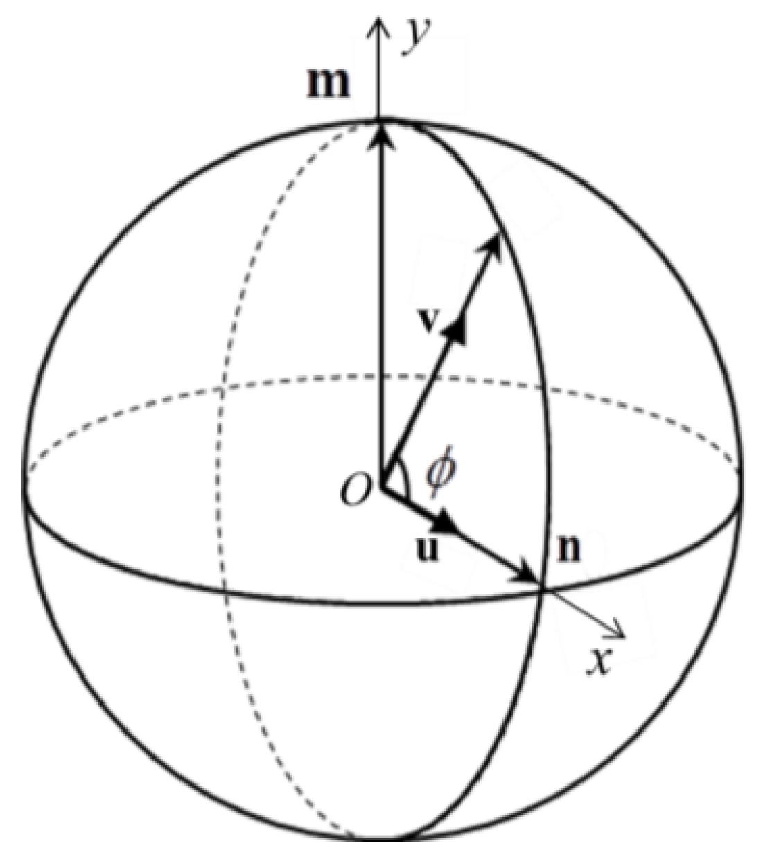
Let us now associate the 3D-geometric approach to the problem, by drawing the Poincaré unit ball of Poincaré vectors (in SR relativistic permitted velocities) (Figure 1). I anticipate that if we consider a P-sphere of Poincaré vectors v with a same, given, modulus v, it will be mapped by a pure boost of vector u to an oblate ellipsoid. For demonstrating this assertion, we shall refer first to a diametrical section of the Poincaré sphere, determined by the Poincaré vector u of the boost and some Poincaré vector v and let us denominate by n and m the unit vectors parallel and perpendicular to u, respectively, and by the angle between u and v (Figure 1). The corresponding Poincaré vector w (outcoming from the boost u) is given by Equation (7). Its projection on u is:
and its projection perpendicular to u:
Finally, Equation (7) may be put in the form:
We shall establish now which is the geometrical locus of the top of the Poincaré vector w for a given u and a given modulus of v, i.e., the geometrical locus of the top of the resultant Poincaré vectors w corresponding to all of the Poincaré vectors v of modulus v and situated in the plane (u, v), or, equivalently, in the plane (n, m).The cartesian coordinates of this geometrical locus are:
By eliminating the parameter , one obtains:
which is the equation of a conic:
Let us process this equation towards the canonical form:
that is it represents an ellipse with the center displaced from origin of the coordinate system along the x axis (direction u). Making the change of variables:
we get the canonical form of this ellipse:
The characteristics of this ellipse are:
- -
- the center displaced from the origin of the coordinate system by:in the sense of the vector u,
- -
- minor semiaxis:
- -
- major semiaxis:
- -
- eccentricity:
If we want to see now how is modified a whole P-sphere by a boost of Poincaré vector u, or, equivalently, by the Poincaré vector’s composition law, Equation (2), we have to consider all the possible corresponding planes (v, u) intersecting along the direction u, i.e., to rotate in Figure 1 the circular section (n, m) around the n axis. The corresponding Lorentz modified P- surface will be an ellipsoid of revolution around u, i.e., with the axis of symmetry along u. Thus, the sphere of all Poincaré vectors of a given, fixed, modulus v, is mapped into an ellipsoid:
with the center displaced with respect to that of the sphere by an amount given by Equation (16).
The compression factor of this ellipsoid:
is smaller than one, so that the ellipsoid is oblate with respect to its axis of symmetry, i.e., with respect to the direction of the boost u.
In SR that means that any sphere of all the velocities v with a same, given, modulus, v, corresponding to the observer , will be mapped by a pure boost of velocity u to an oblate ellipsoid, i.e., it will be seen by the observer as an oblate ellipsoid.
The same results are valid in PT, for the action of an orthogonal dichroic device of strength on a P-sphere [3,36]. Any P-sphere is mapped by a dichroic device into a P-ellipsoid. This ellipsoid is also contained in the Poincaré sphere; it cannot protrude the Poincaré sphere due to the condition of non-overpolarizability (). The equation of this ellipsoid is Equation (20) with instead of u and instead of v.
Moreover, the same results are valid in all of the fields and problems whose underpinning algebra is that of Lorentz transformation, e.g., multilayer optics [18,19,20,21,22,23,24], geometrical optics [25,26], laser cavities [27], and quantum optics [28]. After identifying the corresponding Poincaré vectors, one applies Equation (7), which leads to the same conclusions, in physical terms corresponding to the investigated fields. This has been already done in PT [36], where the mapping of P-spheres in P-ellipsoids follows Equation (20), with , , and (instead of v, u, w) the modules of the corresponding Poincaré vectors.
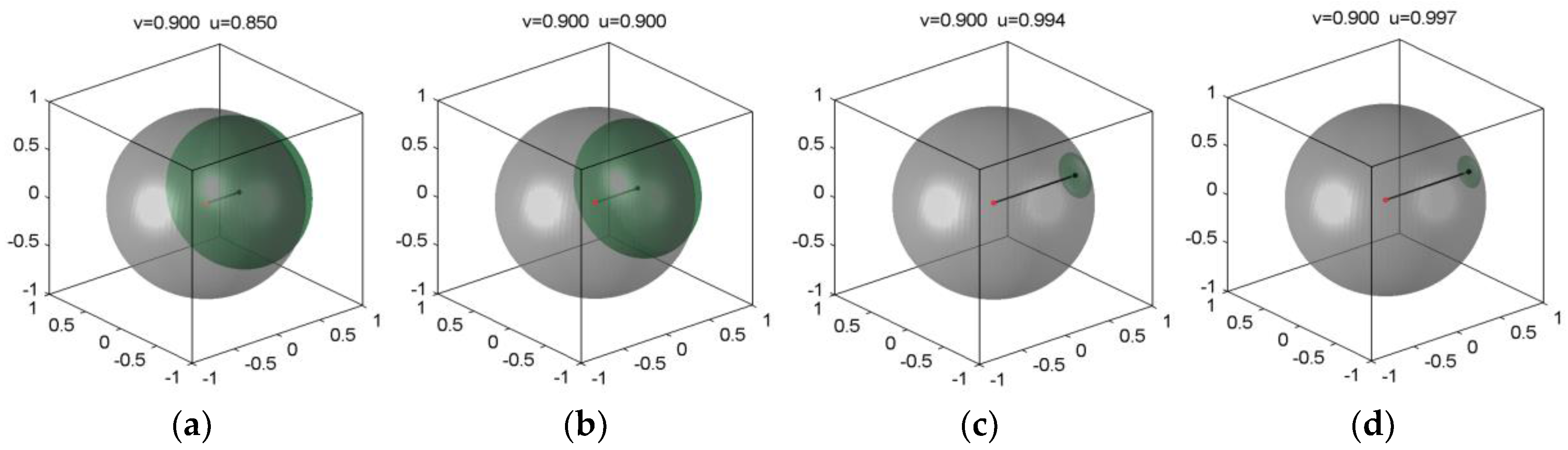
In the next section I shall illustrate, in the 3D space of Poincaré vectors (in SR this is the space of velocities), how the P-ellipsoid is modified when the radius v of the P-sphere and the strength u of the boost change. Besides a better insight in this 3D representation, a surprising aspect will arise. For u and v tending both to 1 (in SR that means both parameters in the ultrarelativistic range), the P-ellipsoid has a strange behavior: when u is more advanced than v in this tendency, the ellipsoid diminishes to a point near the Poincaré sphere wall (Figure 5); when v is more advanced, on the contrary, the P-ellipsoid grows to the Poincaré sphere, finally overlapping it (Figure 6).
4. Behavior of the Ellipsoid with the Parameters u and v
A first way to bring into light the physical content of these formulas is to graphically take an inner Poincaré sphere, a P-sphere, and to see how it is mapped by Lorentz boosts of various strengths. In SR this comes to take a velocity sphere defined for the inertial reference system and to visualize how it is seen by the observer , for various values of the velocity u of the system with respect to , in a given direction n. The corresponding approach in PT is to take a P-sphere of SOP-s of the same degree of polarization and to visualize how it is deformed, mapped, by orthogonal dichroic devices of various degrees of dichroism (boost of various strengths ).
For fixing the basic ideas of this representation, let us begin with a case when the P-sphere and the corresponding ellipsoid are completely separated. Figure 2 illustrates such a situation for v = 0.40 and u = 0.85. How such a figure should be read? We consider all of the Poincaré vectors of the same modulus, v, with their tips uniformly distributed on the surface of the sphere . The emerging Poincaré vectors (“outgoing from the boost”) have the tips distributed (nonuniformly) on the surface of the ellipsoid. The function of distribution of the outgoing states is a question of topology, which deserves a special analyses; it will not be touched in this paper.
As a first remark: the manifold of Poincaré vectors w resulting by the Poincaré vectors’ composition law for all v with the boost strength u are symmetrically gathered together around the direction of the boost u. In SR, this is a holistic expression of the “head-light effect” [41] or “forward collimating effect” [42], emphasized in high energy elementary particle reactions [42]. Such a global view of the forward collimating effect is not known in SR.
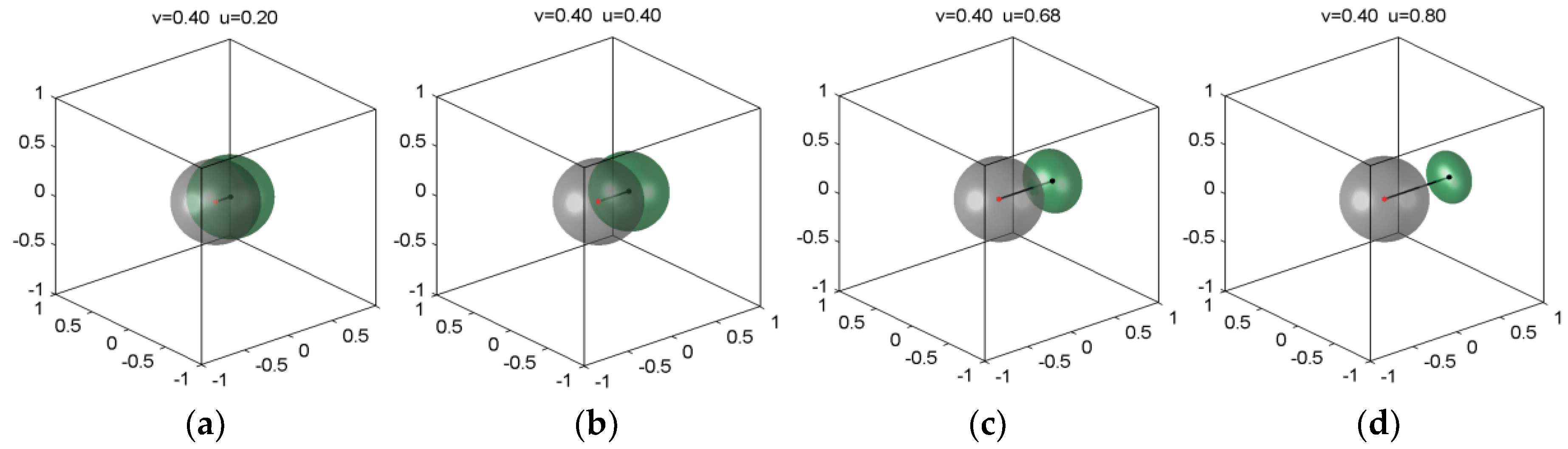
In Figure 2, we have chosen a case when the strength of the boost, u, is high enough with respect to the radius v of the P-sphere for taken out completely the ellipsoid from its corresponding P-sphere.Let us consider now the effect of gradually increasing the strength of the boost, u, on the dimensions, shape, and position of the ellipsoid corresponding to a given P-sphere, i.e., for v fixed (Figure 3). A first global aspect is that as u increases, the ellipsoid becomes smaller and smaller, flatter and flatter, and its center goes farther and farther from the center of the sphere.
At low values of u, the ellipsoid cuts the corresponding P-sphere. In Figure 3a (v = 0.40, u = 0.20), the rear surface of the ellipsoid is still behind the center of the sphere. The corresponding Poincaré vectors, w, are still oriented towards this rear surface (opposite to u). Increasing u (v = 0.40, u = 0.40, Figure 3b), the last rear point of the ellipsoid touches the center of the sphere; for this point w = 0. For higher boost strength, all of the emergent Poincaré vectors corresponding to the given, initial, P-sphere are oriented forward with respect to u, i.e., u is high enough to make this conversion. From Figure 3b, Equations (16) and (17) this happens for:
equation whose positive solution is u = v. It is worth to note that this particular result is identical with the corresponding classical (Galilean, if we refer to kinematics) one. All of the modules w of the Poincaré vectors corresponding to the rear surface of the ellipsoid which lies in the sphere are smaller than v, and all the other greater than v.
Increasing further u, the ellipsoid is pushed farther (Figure 3c) and becomes tangent (exterior) to the sphere . This happens for:
In this case (Figure 3c) the strength of the boost, u, is high enough to convert the last Poincaré vector of the P-sphere, namely that antiparallel with u, in a parallel one, . Only for both u and v very small this equation leads to the classical result: .
Increasing further the strength u of the boost, the ellipsoid of emerging Poincaré vectors w is pushed farther and farther (Figure 3d). Referring to SR (but having in mind the problem of the specific of the Lorentz transformation in its whole generality discussed here), in the Galilean case, the sphere can be pushed at infinity in the velocity space without any deformation. Here, in the relativistic case, it can be pushed only up to the relativistic velocity enclosure, which is up to the wall of the Poincaré sphere. Therefore, its behavior when u increases is quite another one: the sphere is deformed to an ellipsoid and this velocity ellipsoid becomes smaller and smaller and flatter and flatter.
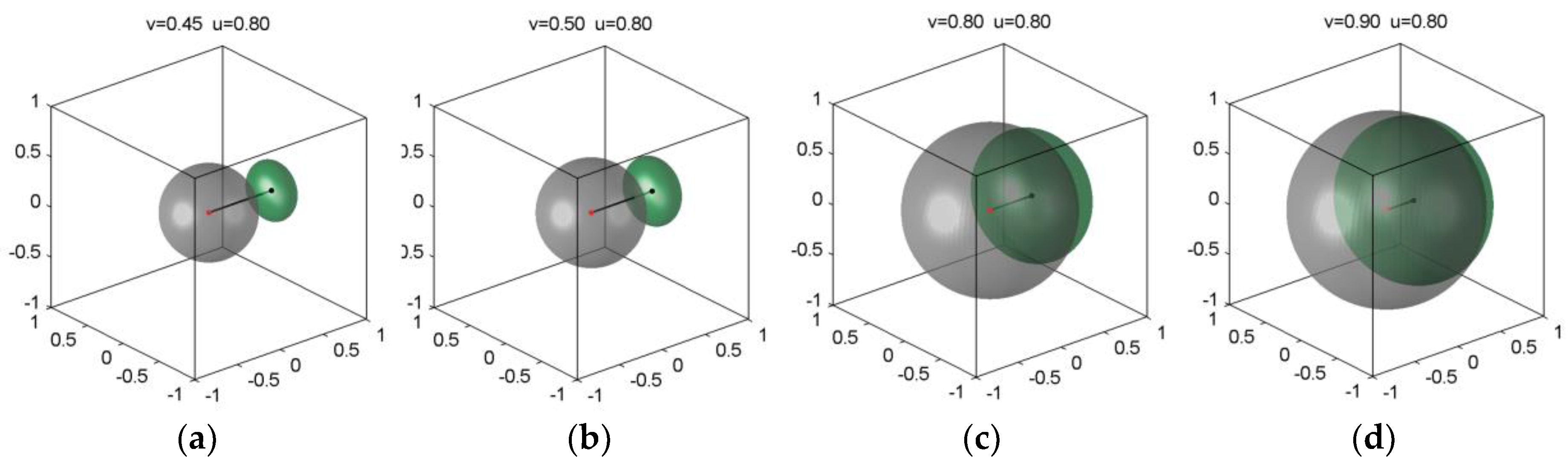
Let us consider now another sequence of situations (Figure 4): we will keep constant the value of the boost’s strength u, and increase gradually the radius v of the P-sphere, . Let us start with a relative high level of u, which has been already reached in the sequence illustrated in Figure 3, namely u = 0.80.
As v increases, the ellipsoid grows back and returns towards the center of the sphere. The ellipsoid overlaps more and more the sphere (Figure 4a–d). This somewhat surprising behavior is, nevertheless, quite understandable. It is expected that a given boost of strength u has a feebler Lorentzian effect on a greater P-sphere than on a smaller one. From Equations (16) and (17), we get:
for the highest w that can be reached in each situation. That means that the ellipsoid can never protrude the Poincaré sphere , in accordance with the constraint Equation (1) physically supported by the second postulate in SR, by the non-overpolarizability condition in PT, by the non-overreflectivity condition in ML, etc. On both sets of figures, Figure 3 and Figure 4, one can notice the interplay between the displacement of the center of the ellipsoid, , and the value of its minor semiaxis, : when one of them increases, the other decreases for ensuring the restriction of Equation (24), in other words, keeping the whole ellipsoid in the Poincaré sphere .
But the strangest behavior of the ellipsoid at the variations of both u and v becomes only now.
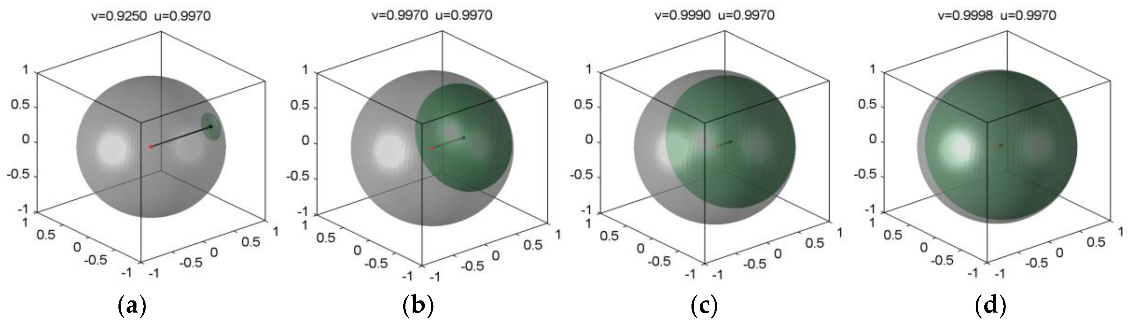
Starting with the last sequence of those presented in Figure 4, i.e., with the highest values of both u an v we have reached until now (Figure 4d, v = 0.90) we shall recommence increasing the values of the boost’s strength, u. The evolution of the ellipsoid repeats the stages represented in Figure 3 at the new level of v. Again, the ellipsoid is pushed towards the wall of the Poincaré sphere; it becomes smaller and smaller and flatter and flatter (see Figure 5). Finally, at the new level of u, namely 0.997, we recommence increasing v, the ellipsoid comes back towards the origin of Poincaré space and becomes bigger and bigger tending finally to overlap the whole sphere (Figure 6d). When the input P-sphere tends to the Poincaré sphere , the output P-ellipsoid tends also to the Poincaré sphere , irrespective of the strength of the Lorentz boost u, accordingly to the second postulate in SR, the non-overpolarizability and the non-overreflectivity conditions in PT and MT, respectively.
This process of increasing and decreasing with u at given v, and, conversely, of decreasing and increasing with v at a given u can be infinitely repeated at higher and higher levels of u and v tending to 1. A deeper analysis of this divergent behavior can be performed by representing the functions which give the dependence of the ellipsoid’s displacement and semiaxis on the parameters u and v. We shall see that these functions, quasilinear in the range u, v→0 (Galilean limit in SR) become strongly nonlinear and indefinite in the range u, v→1 (extreme relativistic limit in SR).
5. Nonlinearity and Indefinitness of the Ellipsoid Characteristics as Functions of u and v
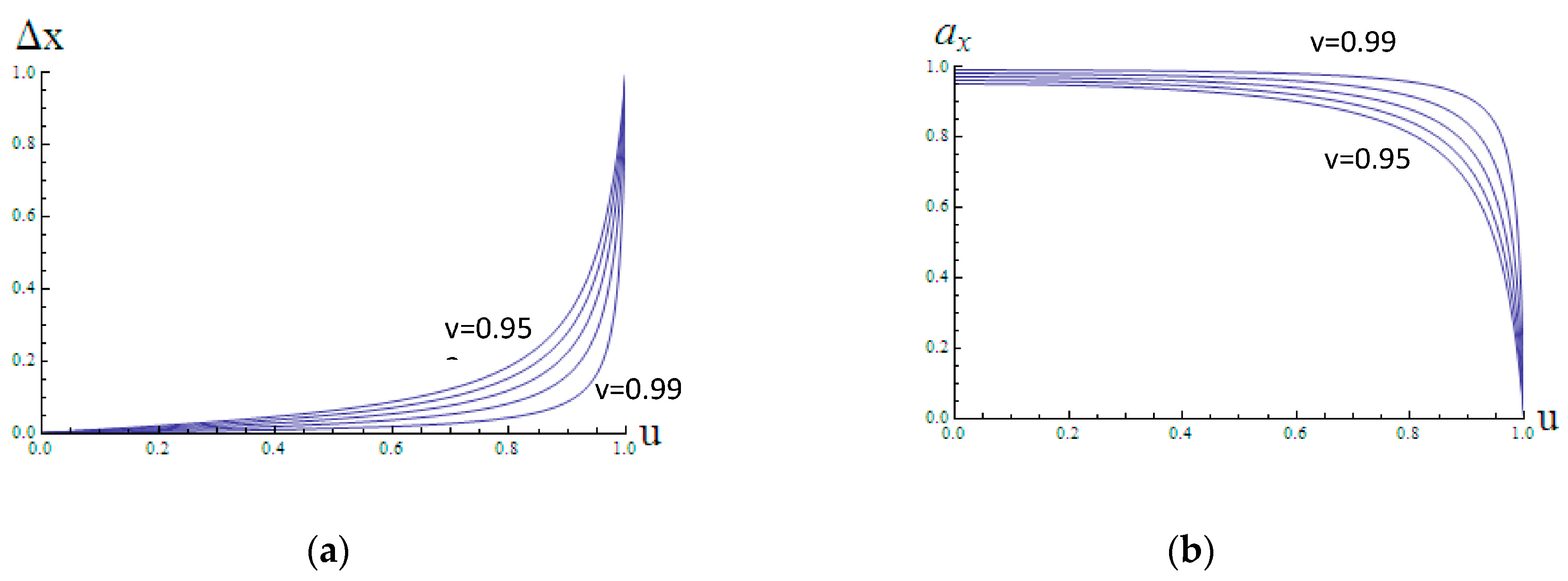
All of the functions , , , given in Equations (16)–(19) are nonlinear and become indefinite for u and v tending together to 1. For analyzing these aspects, we shall start with the behavior of two of the relevant quantities, let say and , as functions of one of the variables, let say u, at various values of the second variable v, seen as parameter (Figure 7).
For low values of the radius v of the Poincaré sphere :
But, as the radius v of the Poincaré sphere increases:
These behaviors become more prominent for very large values of the radius v of the Poincaré sphere (in SR, in the extreme relativistic regime, let say of the rank of v > 0.95) (Figure 8):
- -
- increases very slowly up to the critical value of u, and after this value starts, suddenly, to grow very abruptly with u (Figure 8a); and,
- -
- similarly, decreases from the value v very slowly with u up to the critical value of u, and after this value becomes suddenly to decrease abruptly to zero (Figure 8b).
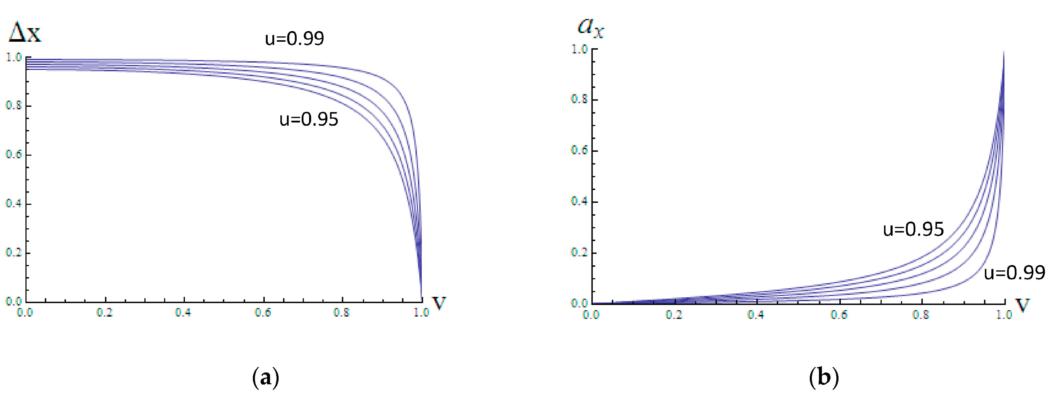
An intriguing aspect of these relationships arises if we represent, complementary to Figure 8, Δx and as functions of u at various values of v seen as parameter (Figure 9).
If we judge on the basis of Figure 8a, in the limit , (ultrarelativistic limit in SR) we get the value 1 for , whereas if we judge on the basis of Figure 9a, for the same extreme case , , we get the value zero for . The same situation arises for ellipsoid’s semiaxis : If we judge on the basis of Figure 8b, in the limit , we get the value zero for , whereas if we judge on the basis of Figure 9b, for the same extreme case , , we get the value 1 for . We have an expressive illustration of these divergent behaviors, especially in the series of images of Figure 5 and Figure 6. In the first of them, the ellipsoid diminishes to a point, i.e., tends to zero, whereas in the second, the ellipsoid tends to the Poincaré sphere, tends to 1. The limit depends on which of the parameters u and v is in advance in this process, in other words on the way of this process. In fact, both the function given in Equations (16) and (17) are indefinite for both , that is, in SR for the ultrarelativistic limit of both velocities.
It is remarkable that the expressions of and as functions of u, v can be obtained one from the other by interchanging u and v (Equations (16) and (17)). By consequence the graph as function of v with u as parameter (Figure 9a) coincides with the graph of as function of u with v as parameter (Figure 8b). The behavior of (and ) is similar (but inversed) with that of . Thus, an analysis of the nonlinearity and indefiniteness in behavior of for is completely relevant for all of the characteristics of the ellipsoid.
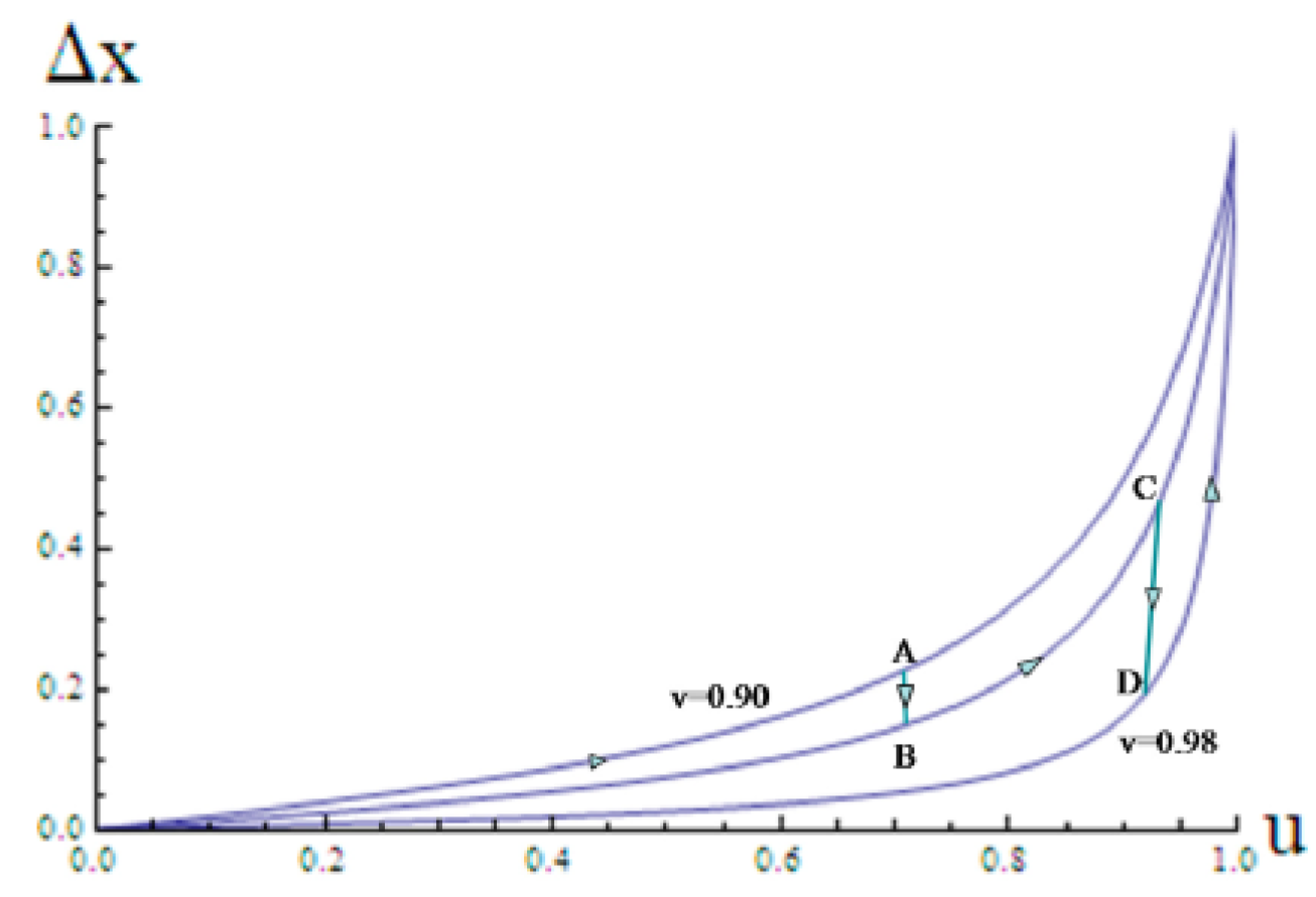
We can grasp a deeper insight on what happens in the range as follows (Figure 10): Let us increase the strength of the boost, u, at a low or moderate value of the radius v of the Poincaré sphere , e.g., up to the point A, and then, keeping constant this value of u, begin to increase the value of v. On the graph in Figure 10, this comes to get down on a line parallel to the axis up to, let say, the point B. The , which has grown in the first step (OA), goes back, diminishes, in this new step (AB). We have to note that, if we increase drastically the value of v, the point B can get down drastically, leading to , that is cancelling the effect of the previous growth of u (on the OA range). Let us further keep constant the value of v corresponding to the point B and increase again the value of u. We will go up on the curve BC (an “iso-v”), up to a point C. The value of will increase again. A further increase of v (the segment CD) implies again a decrease of . If we want to reach the absolute limit , we would continue endless this interplay: a raise in value of u, implies an increase of , but it will be followed by a raise of v, which implies a decrease of . As we go closer to 1 by both u and v, the jump in the two steps (increasing u, increasing v), visualized by the lengths of the vertical segments AB, CD, etc., gets nearer to the step , (the limit of for and the limit of for ).
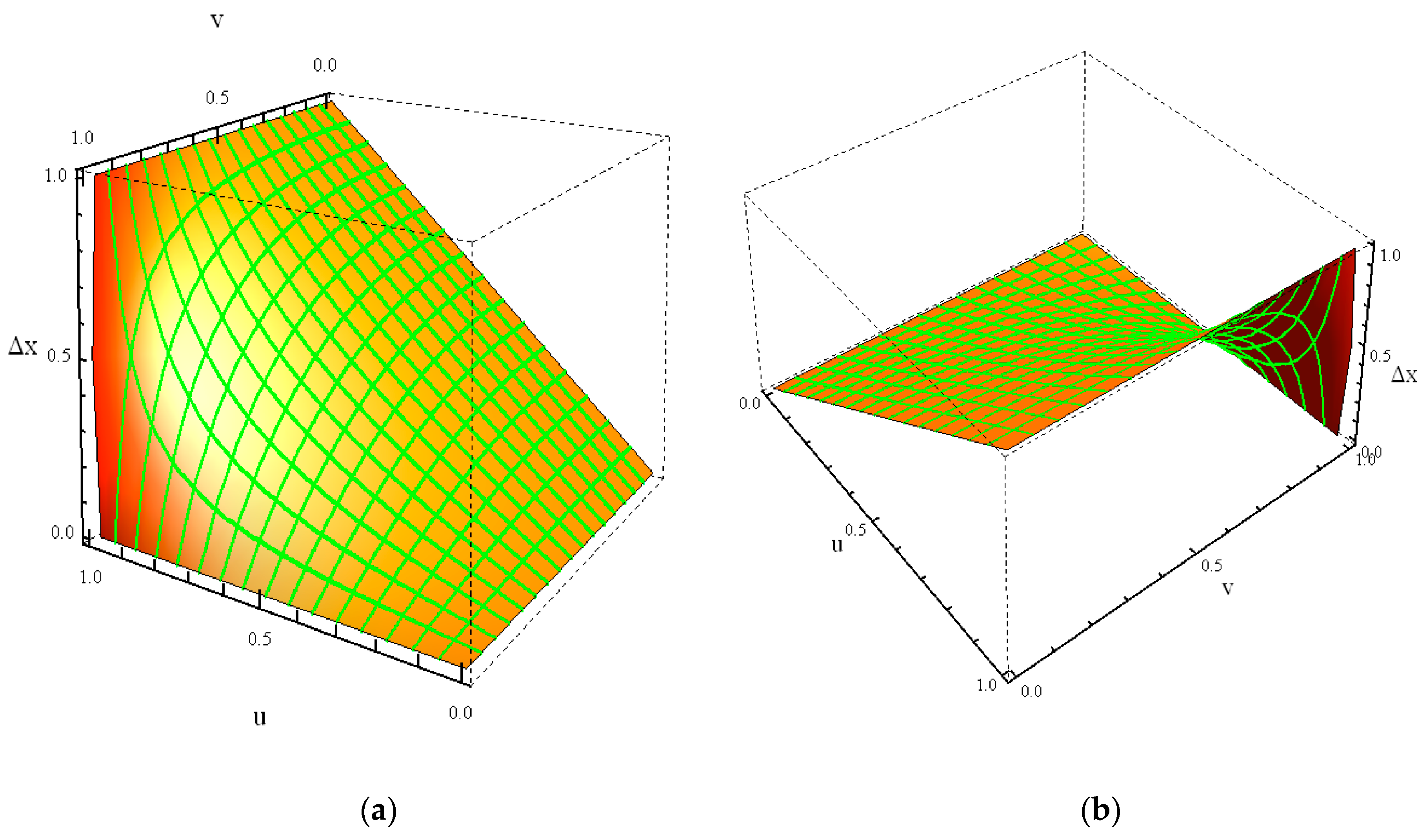
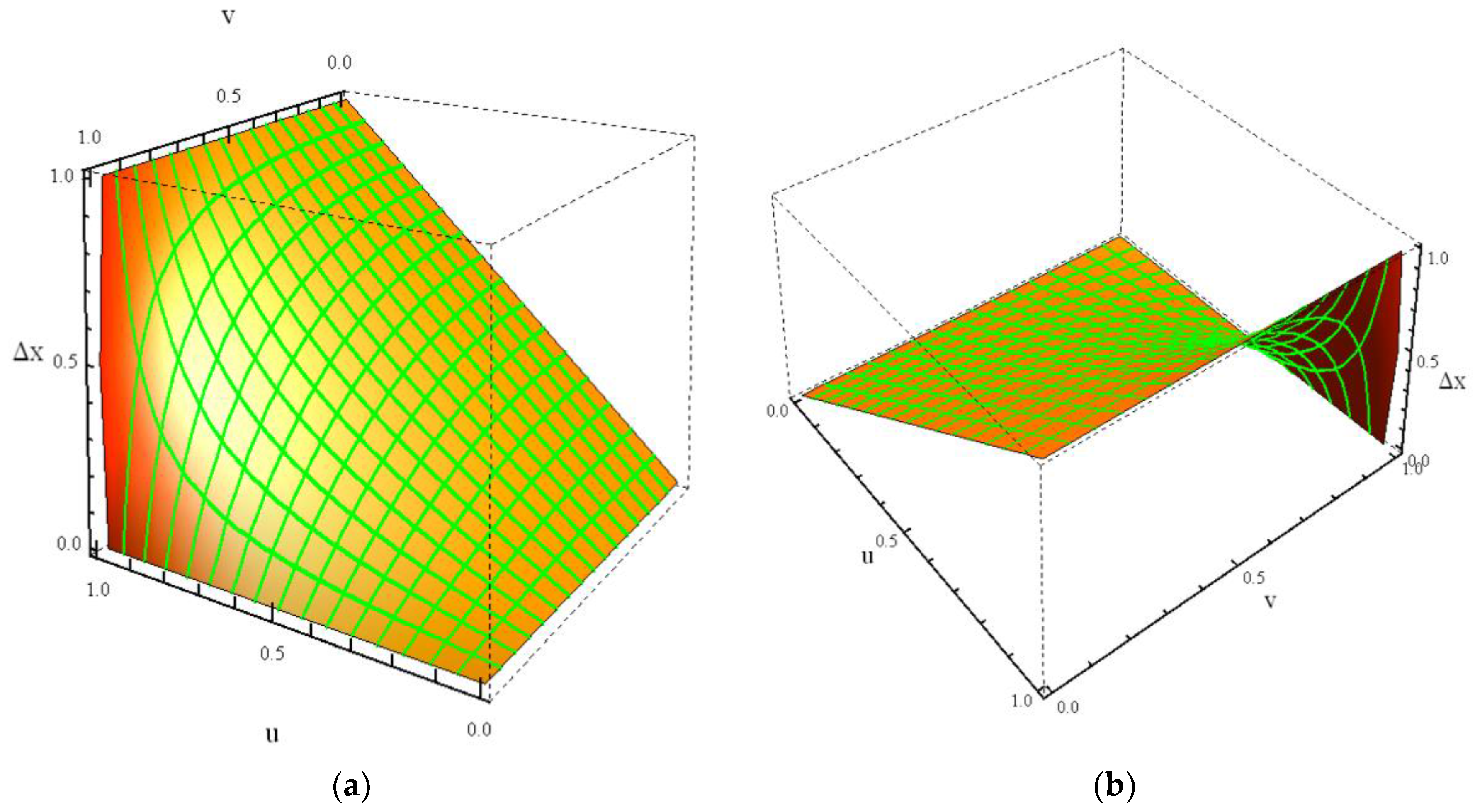
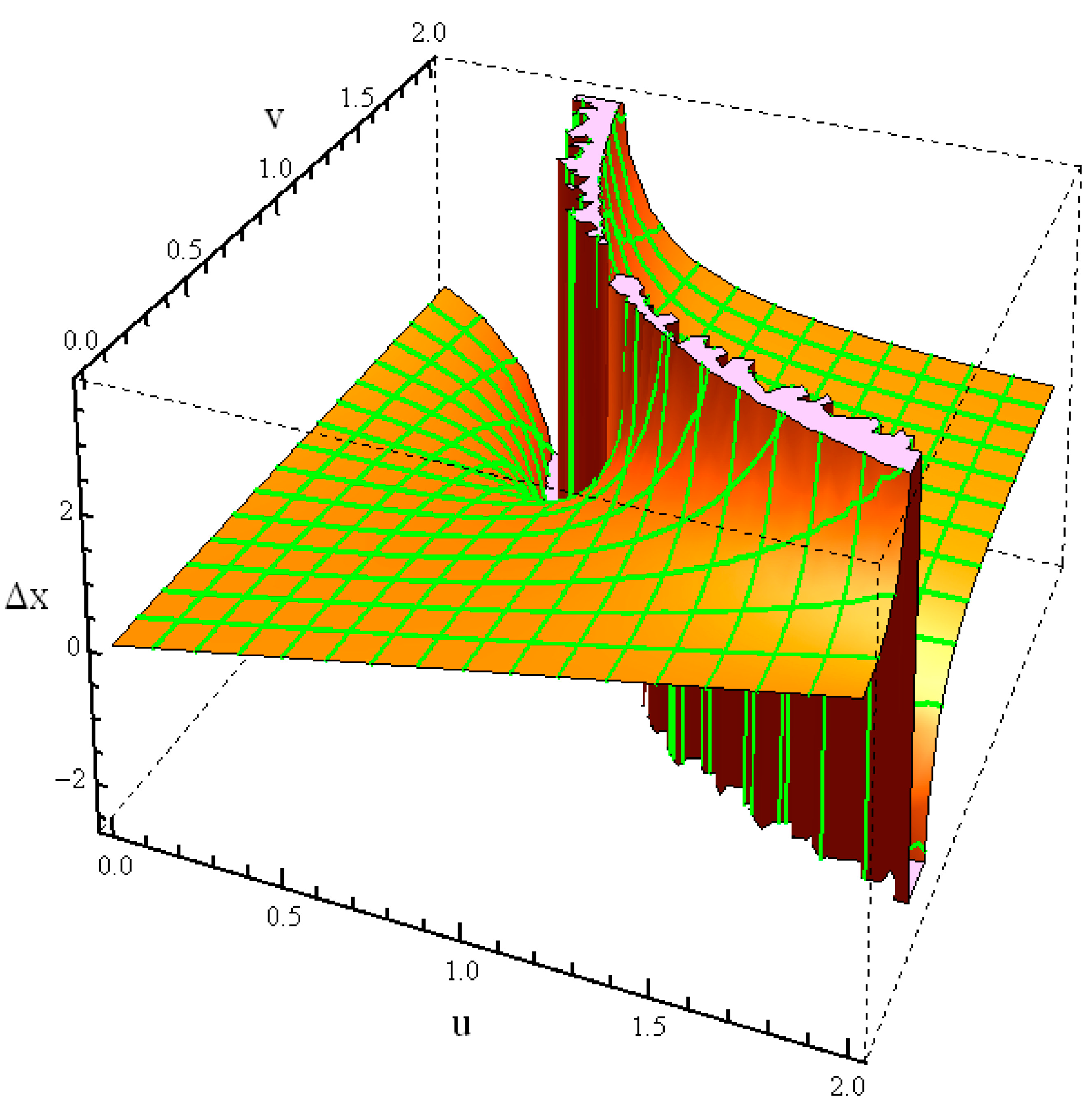
Figure 11 provides a 3D representation of the function from two different perspectives. Following each of the two crossed systems of level lines, one of them at v = const., the second at u = const., one can reach a global view of the aspects pointed out above in analyzing the graphs of Figure 7, Figure 8, Figure 9.
In Figure 11a, I have brought in the foreground the ultrarelativistic (in SR terms) region of the function. Near the right-lower corner (u = 0, v = 0) of the (1,1,1) cube, the function has a quasi-classical (Galilean) behavior. The grating of crossed level lines is practically a rectangular one; varies almost linearly with both u and v. On the contrary, in the left-front side of the cube, the system of level lines reveals the nonlinearity and indefiniteness of the function in the (again in SR terms) extreme relativistic region u, v→1. The second perspective (Figure 11b) emphasizes the contortioned behavior of the function that is imposed by the physical constraints of the second postulate, non-overpolarizability, etc.
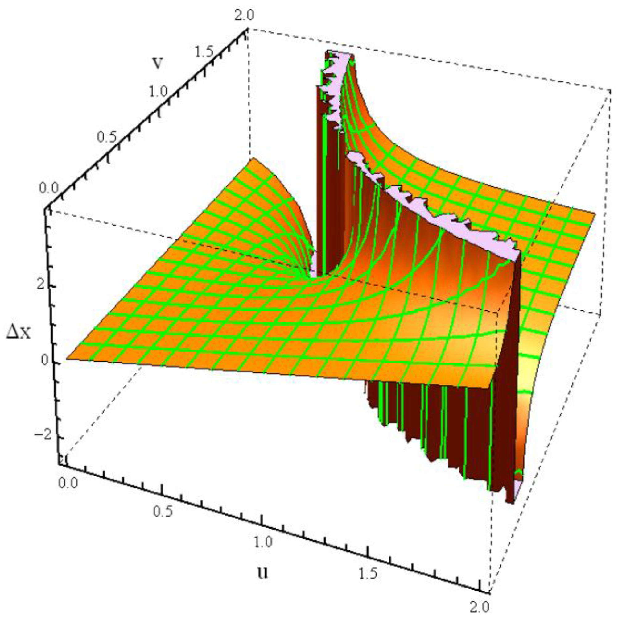
This behavior of the function appears at its best if it is presented, as I have done in Figure 12, symmetrically around the value 1 of both variables u and v, which is extending it in the unphysical region [1 ÷ 2] of the parameters (u, v), or, as one of reviewers has noted, deeply into the tachyonic regime. Maybe this view could constitute a challenge for the mathematicians who would continue the analyses of this Poincaré representation of Lorentz transformation, for which the functions given by Equations (16) and (17) are fundamental.
6. Conclusions
For more than a century, when we try to get an intuitive grasp on Lorentz transformations, we make appeal to the geometrical representation of these transformations in the quadridimensional space of events, suggested by Poincaré, introduced by Minkovski in 1907, and developed in the frame of the theory of relativity.
Fifteen years before that, in 1992, Poincaré introduced in polarization theory the sphere that bears now his name, in order to represent the states of light polarization. Initially neglected for about two decades, the Poincaré sphere became a powerful geometric tool in polarization theory, with no interference with the theory of relativity. In the last decade, in the frame of this geometric representation was elaborated the P-sphere approach to the interactions of various polarization devices/media with polarized light. One of these interaction, namely that of orthogonal dichroic devices with polarized light is governed by a Lorentz transformation. By consequence, the P-sphere approach and its geometrical frame, the Poincaré sphere, may be transferred in relativity, as well as in all the fields whose mathematical underground is that of Lorentz transformations, what I have done in this paper. This approach could be denominated Poincaré representation of Lorentz transformations (bearing in mind, of course, that it operates at the level of Poincaré vectors).
Particularly, if we refer to relativity, this geometric tool operates in the velocity space and is an alternative to the Minkowskian one, which operates in the space of events. When one constructs a representation of a velocity (more exactly rapidity) space starting from a Minkowski diagram, one imports in this representation the drawbacks, the limits, of these diagram—the unavoidable absence of (at least) one spatial dimension—reducing, this way, the 3D hypercones to 2D cones, the hyper-hyperboloids to hyperboloids, the spheres to circles, etc., as a price for the geometric intuitive grasp of the Lorentz transformations. The actual models (representations) of the relativistic velocity space (hyperboloid, Poincaré disk, paraboloid, Klein disc) are all 2D spaces, as a consequence of the fact that they were constructed starting from the geometric representations of the 2 + 1 Minkowskian space of events. But, if the world of physical events is naturally a quadridimensional one, the world of velocities is a three-dimensional one and a 3D approach to the problem of the relativistic behavior of velocities is absolutely possible. Of course, we have to pay a price for this advantage of a 3D approach: the Minkowskian character of the space-time is reflected at the level of relativistically allowed velocities in the fact that these velocities are composed in a contortioned manner, as we have seen in detail above.
The ultimate reason of this contortion (as well as of that of the Minkowski metric) is, evidently, the constraint (Equation (1)), which is common for all of the fields and problems that we have listed in the introduction. In SR, this constraint has a counterintuitive origin: the second postulate. In all of the other fields, it originates in physical restrictions that are in perfect accordance with our intuition: the degree of polarization, the reflection coefficient, etc., cannot overpass unity, by their very definition.
Acknowledgments
I am grateful to all the three referees for their suggestions that resulted in a substantial improvement of the manuscript.
Conflicts of Interest
The author declares no conflict of interest.
References
- Barakat, R. Theory of the coherency matrix for light of arbitrary spectral bandwidth. J. Opt. Soc. Am. 1963, 53, 317–323. [Google Scholar] [CrossRef]
- Gil, J. Polarimetric characterization of light and media. Eur. Phys. J. Appl. Phys. 2007, 40, 1–47. [Google Scholar] [CrossRef]
- Gil, J.J.; Ossikovski, R. Polarized Light and the Mueller Matrix Approach; CRC Press: Boca Raton, FL, USA, 2016. [Google Scholar]
- Savenkov, S.V.; Sydoruk, O.; Muttiah, R.S. Conditions for polarization elements to be dichroic and birefringent. J. Opt. Soc. Am. A 2005, 22, 1447–1452. [Google Scholar] [CrossRef]
- Angelsky, O.V.; Hanson, S.G.; Zenkova, C.Y.; Gorsky, M.P.; Gorodyns’ka, N.V. On polarization metrology of the degree of coherence of optical waves. Opt. Express. 2009, 17, 15623–15634. [Google Scholar] [CrossRef] [PubMed]
- Angelsky, O.V.; Polyanskii, P.V.; Maksimyak, P.P.; Mokhun, I.I.; Zenkova, C.Y.; Bogatyryova, H.V.; Felde, C.V.; Bachinskiy, V.T.; Boichuk, T.M.; Ushenko, A.G. Optical measurements: Polarization and coherence of light fields. In Modern Metrology Concerns—Monography; Coccco, L., Ed.; In Tech: Rijeka, Croatia, 2012. [Google Scholar]
- Barakat, R. Bilinear constraints between elements of the 4 × 4 Mueller-Jones transfer matrix of polarization theory. Opt. Commun. 1981, 38, 159–161. [Google Scholar] [CrossRef]
- Takenaka, H. A unified formalism for polarization optics by using group theory. Nouv. Rev. Opt. 1973, 4, 37–41. [Google Scholar] [CrossRef]
- Kitano, M.; Yabuzaki, T. Observation of Lorentz-group Berry phases in polarization optics. Phys. Lett. A 1989, 142, 321–325. [Google Scholar] [CrossRef]
- Pellat-Finet, P. What is common to both polarization optics and relativistic kinematics? Optik 1992, 90, 101–106. [Google Scholar]
- Opatrnỳ, T.; Peřina, J. Non-image-forming polarization optical devices and Lorentz transformations—An analogy. Phys. Lett. A 1993, 181, 199–202. [Google Scholar] [CrossRef]
- Han, D.; Kim, Y.S. Polarization optics and bilinear representation of the Lorentz group. Phys. Lett. A 1996, 219, 26–32. [Google Scholar] [CrossRef]
- Han, D.; Kim, Y.S.; Noz, M.E. Stokes parameters as a Minkowskian four-vector. Phys. Rev. E 1997, 56, 6065–6076. [Google Scholar] [CrossRef]
- Kim, Y.S. Lorentz group in polarization optics. J. Opt. B 2000, 2, R1–R5. [Google Scholar] [CrossRef]
- Morales, J.A.; Navarro, E. Minkowskian description of polarized light and polarizers. Phys. Rev. E 2003, 67, 026605. [Google Scholar] [CrossRef] [PubMed]
- Tudor, T. Interaction of light with the polarization devices: A vectorial Pauli algebraic approach. J. Phys. A Math. Theor. 2008, 41, 1–12. [Google Scholar] [CrossRef]
- Lages, J.; Giust, R.; Vigoureux, J.M. Composition law for polarizers. Phys. Rev. A 2008, 78, 033810. [Google Scholar] [CrossRef]
- Vigoureux, J.M. Use of Einstein’s addition law in studies of reflection by stratified planar structures. J. Opt. Soc. Am. A 1992, 9, 1313–1319. [Google Scholar] [CrossRef]
- Vigoureux, J.M.; Grossels, Ph. A relativistic-like presentation of optics in stratified planar media. Am. J. Phys. 1993, 61, 707–712. [Google Scholar] [CrossRef]
- Monzón, J.J.; Sánchez-Soto, L.L. Fully relativisticlike formulation of multilayers optics. J. Opt. Soc. Am. A 1999, 16, 2013–2018. [Google Scholar] [CrossRef]
- Monzón, J.J.; Sánchez-Soto, L.L. Fresnel formulas as Lorentz transformations. J. Opt. Soc. Am. 2000, 17, 1475–1481. [Google Scholar] [CrossRef]
- Monzón, J.J.; Sánchez-Soto, L.L. Optical multilayers as a tool for visualizing special relativity. Eur. J. Phys. 2001, 22, 39–51. [Google Scholar] [CrossRef]
- Giust, R.; Vigoureux, J.M. Hyperbolic representation of light propagation in a multilayer medium. J. Opt. Soc. Am. A 2002, 19, 378–384. [Google Scholar] [CrossRef]
- Giust, R.; Vigoureux, J.M.; Lages, J. Generalized composition law from 2 × 2 matrices. Am. J. Phys. 2009, 77, 1068–1073. [Google Scholar] [CrossRef]
- Başkal, S.; Georgieva, E.; Kim, Y.S.; Noz, M.E. Lorentz group in classical ray optics. J. Opt. B Quantum Semiclass. Opt. 2004, 6, 4554. [Google Scholar]
- Başkal, S.; Kim, Y.S. Problems of measurement in Quantum Optics and Informatics, the Language of Einstein Spoken by Optical Instruments. Opt. Spectrosc. 2005, 99, 443–446. [Google Scholar] [CrossRef]
- Başkal, S.; Kim, Y.S. Wigner rotations in laser cavites. Phys. Rev. E 2002, 66, 026604. [Google Scholar] [CrossRef] [PubMed]
- Han, D.; Hardekopl, E.E.; Kim, Y.S. Thomas precession and squeezed states of light. Phys. Rev. A 1989, 39, 1269. [Google Scholar] [CrossRef]
- Ungar, A.A. Analytic Hyperbolic Geometry. Mathematical Foundation and Applications; World Scientific: Hackensack, NJ, USA, 2005. [Google Scholar]
- Ungar, A.A. Thomas rotation and the parametrization of the Lorentz transformation group. Found. Phys. Lett. 1988, 1, 57–68. [Google Scholar] [CrossRef]
- Feynman, R.P.; Leighton, R.; Sands, M. The Feynman Lectures on Physics; Addison-Wesley: London, UK, 1977; Volume I, Chapter 15. [Google Scholar]
- Tudor, T. On a quasi-relativistic formula in polarization theory. Opt. Lett. 2015, 40, 1–4. [Google Scholar] [CrossRef] [PubMed]
- Williams, M.W. Depolarization and cross polarization in ellipsometry of rough surfaces. Appl. Opt. 1986, 25, 3616–3622. [Google Scholar] [CrossRef] [PubMed]
- DeBoo, B.; Sasian, J.; Chipman, R. Degree of polarization surfaces and maps for analysis of depolarization. Opt. Express. 2004, 12, 4941–4958. [Google Scholar] [CrossRef] [PubMed]
- Ferreira, C.; José, I.S.; Gil, J.J.; Correas, J.M. Geometric modeling of polarimetric transformations. Mono. Sem. Mat. G. de Galdeano 2006, 33, 115–119. [Google Scholar]
- Tudor, T.; Manea, V. The ellipsoid of the polarization degree. A vectorial, pure operatorial Pauli algebraic approach. J. Opt. Soc. Am. B 2011, 28, 596–601. [Google Scholar] [CrossRef]
- Ossikovski, R.; Gil, J.J.; San José, I. Poincaré sphere mapping by Mueller matrices. J. Opt. Soc. Am. A 2013, 30, 2291–2305. [Google Scholar] [CrossRef] [PubMed]
- Gil, J.J.; Ossikovski, R.; San José, I. Singular Mueller matrices. J. Opt. Soc. Am. A 2016, 33, 600–609. [Google Scholar] [CrossRef] [PubMed]
- Tudor, T.; Manea, V. Symmetry between partially polarized light and partial polarizers in the vectorial Pauli algebraic formalism. J. Mod. Opt. 2011, 58, 845–852. [Google Scholar] [CrossRef]
- Poincaré, H. Theorie Mathématique de la Lumière; Carrè: Paris, France, 1892. [Google Scholar]
- Rindler, W. Relativity. Special, General and Cosmological; Oxford University Press: New York, NY, USA, 2006. [Google Scholar]
- Sard, R.D. Relativistic Mechanics; W.A. Benjamin Inc.: New York, NY, USA, 1970. [Google Scholar]
Figure 1.
Poincaré unit ball. Notations.

Figure 2.
A P-sphere and the corresponding ellipsoid (v = 0.40, u = 0.85).
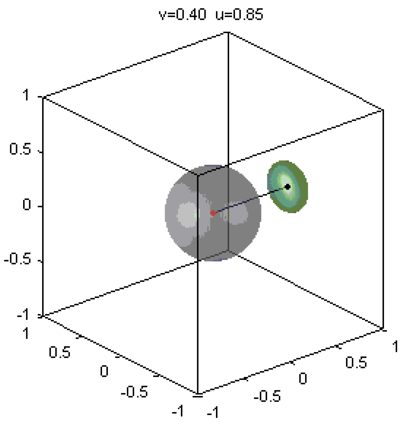
Figure 3.
When the strength of the boost increases the ellipsoid corresponding to a given P-sphere (v = 0.40) is pushed farther and farther and becomes smaller and smaller: (a) u = 0.20; (b) u = 0.40; (c) u = 0.68; (d) u = 0.80.
Figure 3.
When the strength of the boost increases the ellipsoid corresponding to a given P-sphere (v = 0.40) is pushed farther and farther and becomes smaller and smaller: (a) u = 0.20; (b) u = 0.40; (c) u = 0.68; (d) u = 0.80.

Figure 4.
Increasing the radius v of the P-sphere at a given u (u = 0.80), the corresponding ellipsoid becomes greater and greater and comes back to the origin of the Poincaré space: (a) v = 0.45; (b) v = 0.50; (c) v = 0.80; (d) v = 0.90.
Figure 4.
Increasing the radius v of the P-sphere at a given u (u = 0.80), the corresponding ellipsoid becomes greater and greater and comes back to the origin of the Poincaré space: (a) v = 0.45; (b) v = 0.50; (c) v = 0.80; (d) v = 0.90.

Figure 5.
Behavior of the ellipsoid when u increases at a higher level of v (v = 0.900): (a) u = 0.850; (b) u = 0.900; (c) u = 0.994; (d) u = 0.997.
Figure 5.
Behavior of the ellipsoid when u increases at a higher level of v (v = 0.900): (a) u = 0.850; (b) u = 0.900; (c) u = 0.994; (d) u = 0.997.

Figure 6.
Behavior of the ellipsoid when v increases at a higher level of u (u = 0.997): (a) v = 0.925; (b) v = 0.997; (c) v = 0.999; (d) v = 0.9998.
Figure 6.
Behavior of the ellipsoid when v increases at a higher level of u (u = 0.997): (a) v = 0.925; (b) v = 0.997; (c) v = 0.999; (d) v = 0.9998.

Figure 7.
Δx and as function of u, with v as parameter, at low and moderate values of v. (a) upper line v = 0.2, lower curve v = 0.8; (b) lower curve v = 0.2, upper curve v = 0.8.
Figure 7.
Δx and as function of u, with v as parameter, at low and moderate values of v. (a) upper line v = 0.2, lower curve v = 0.8; (b) lower curve v = 0.2, upper curve v = 0.8.
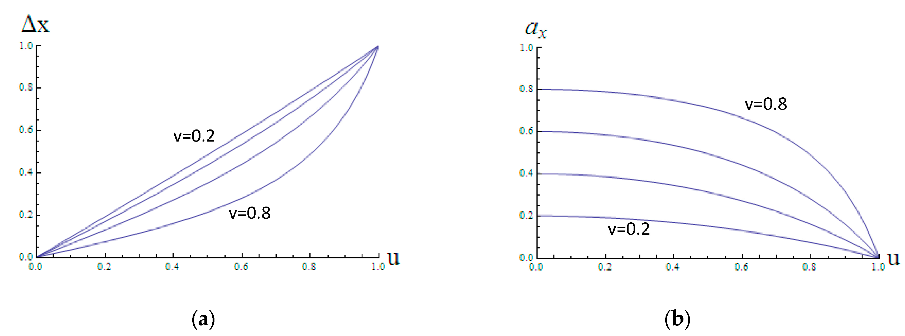
Figure 8.
Δx and as function of u at high values of v. (a) upper curve v = 0.95, lower curve v = 0.99; (b) lower curve v = 0.95, upper curve v = 0.99.
Figure 8.
Δx and as function of u at high values of v. (a) upper curve v = 0.95, lower curve v = 0.99; (b) lower curve v = 0.95, upper curve v = 0.99.

Figure 9.
Δx and as function of v with u as parameter; (a) lower curve u = 0.95, upper curve u = 0.99; (b) upper curve u = 0.95, lower curve u = 0.99.
Figure 9.
Δx and as function of v with u as parameter; (a) lower curve u = 0.95, upper curve u = 0.99; (b) upper curve u = 0.95, lower curve u = 0.99.

Figure 10.
Back and forth play of Δx when u and v increase alternatively toward their extreme limit.
Figure 10.
Back and forth play of Δx when u and v increase alternatively toward their extreme limit.
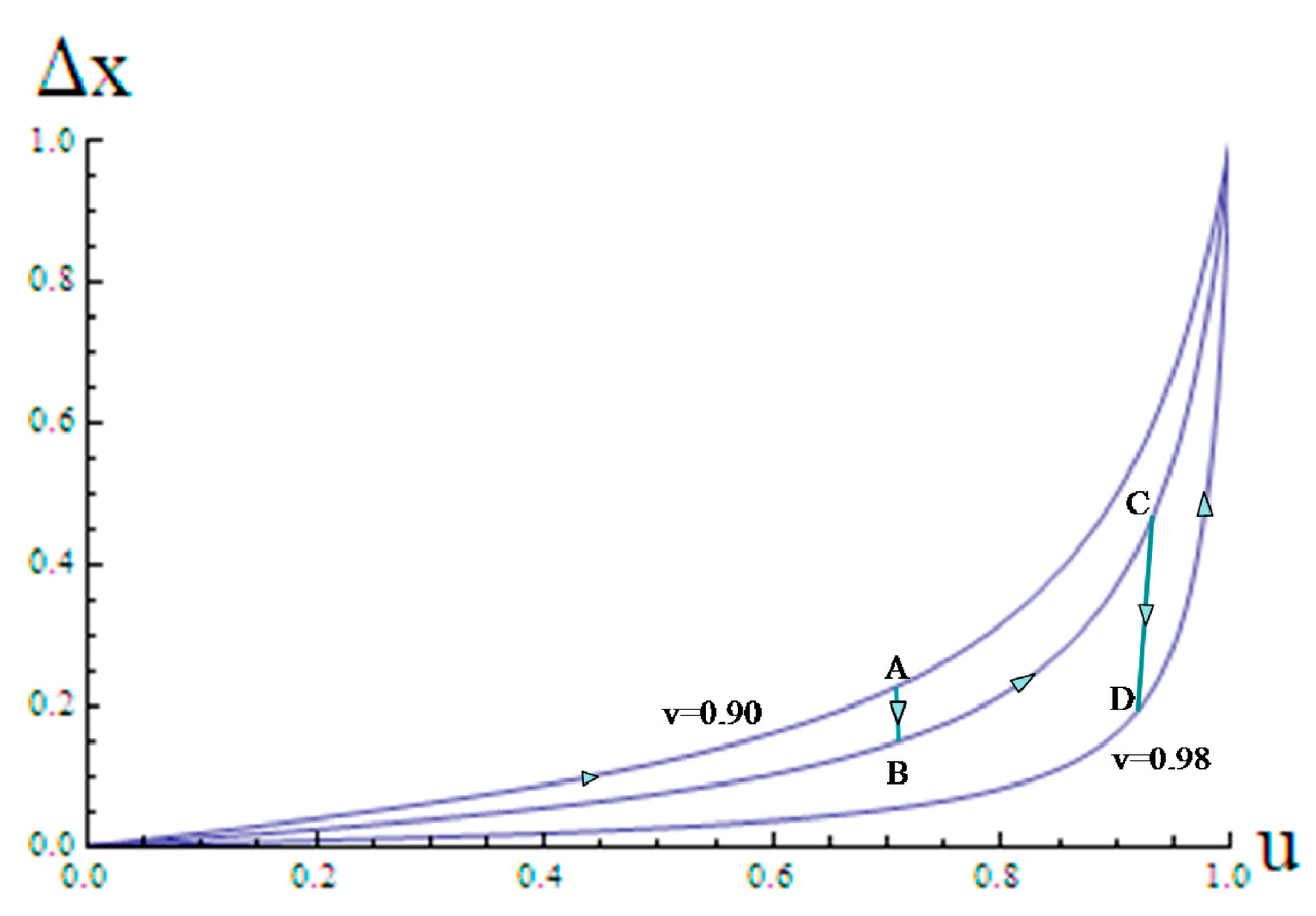
Figure 11.
The function Δx (u, v) in the region of physical interest: (a,b) mean two different perspectives.
Figure 11.
The function Δx (u, v) in the region of physical interest: (a,b) mean two different perspectives.

Figure 12.
A symmetrically extended view of the function Δx (u, v).
© 2018 by the author. Licensee MDPI, Basel, Switzerland. This article is an open access article distributed under the terms and conditions of the Creative Commons Attribution (CC BY) license (http://creativecommons.org/licenses/by/4.0/).
Share and Cite
MDPI and ACS Style
Tudor, T. Lorentz Transformation, Poincaré Vectors and Poincaré Sphere in Various Branches of Physics. Symmetry 2018, 10, 52. https://doi.org/10.3390/sym10030052
AMA Style
Tudor T. Lorentz Transformation, Poincaré Vectors and Poincaré Sphere in Various Branches of Physics. Symmetry. 2018; 10(3):52. https://doi.org/10.3390/sym10030052
Chicago/Turabian StyleTudor, Tiberiu. 2018. "Lorentz Transformation, Poincaré Vectors and Poincaré Sphere in Various Branches of Physics" Symmetry 10, no. 3: 52. https://doi.org/10.3390/sym10030052
Note that from the first issue of 2016, this journal uses article numbers instead of page numbers. See further details here.