Cuckoo Search Algorithm with Lévy Flights for Global-Support Parametric Surface Approximation in Reverse Engineering

Abstract

This paper concerns several important topics of the Symmetry journal, namely, computer-aided design, computational geometry, computer graphics, visualization, and pattern recognition. We also take advantage of the symmetric structure of the tensor-product surfaces, where the parametric variables u and v play a symmetric role in shape reconstruction. In this paper we address the general problem of global-support parametric surface approximation from clouds of data points for reverse engineering applications. Given a set of measured data points, the approximation is formulated as a nonlinear continuous least-squares optimization problem. Then, a recent metaheuristics called Cuckoo Search Algorithm (CSA) is applied to compute all relevant free variables of this minimization problem (namely, the data parameters and the surface poles). The method includes the iterative generation of new solutions by using the Lévy flights to promote the diversity of solutions and prevent stagnation. A critical advantage of this method is its simplicity: the CSA requires only two parameters, many fewer than any other metaheuristic approach, so the parameter tuning becomes a very easy task. The method is also simple to understand and easy to implement. Our approach has been applied to a benchmark of three illustrative sets of noisy data points corresponding to surfaces exhibiting several challenging features. Our experimental results show that the method performs very well even for the cases of noisy and unorganized data points. Therefore, the method can be directly used for real-world applications for reverse engineering without further pre/post-processing. Comparative work with the most classical mathematical techniques for this problem as well as a recent modification of the CSA called Improved CSA (ICSA) is also reported. Two nonparametric statistical tests show that our method outperforms the classical mathematical techniques and provides equivalent results to ICSA for all instances in our benchmark.

1. Introduction

1.1. Surface Approximation in Reverse Engineering

Reverse engineering is a very important research subject that is currently receiving a lot of attention from the scientific and industrial communities. Most of this interest is motivated by its outstanding applications to the design, development, and manufacturing of consumer goods [1,2]. Typical fields of application of reverse engineering include computer design and manufacturing (CAD/CAM) for the automotive, aerospace and ship building industries, biomedical engineering (prosthesis, medical implants), medicine (computer tomography, magnetic resonance), digital heritage, computer animation and video games (motion capture, facial scanning), and many others.

Reverse engineering technology is focused on reconstructing a Computer-Aided Design (CAD) model from a physical part of an existing or already constructed object [3]. Typically, the process starts with the digitization of this physical workpiece through the use of 3D laser scanners or other digitizing devices (e.g., coordinate measuring machines). As a result, a (very large) cloud of data points capturing the underlying geometrical shape of the object is obtained. This point cloud is then transformed into a compact CAD model by means of data fitting techniques [4,5].

Depending on the nature and characteristics of the cloud of data points, two different approaches for data fitting can be used: interpolation or approximation [3]. The former case generates a parametric curve or surface that passes through all data points. In contrast, the approximation techniques generate a curve or surface that only passes near the data points, generally minimizing the deviation from them according to a prescribed energy functional, which usually takes the form of a least-squares minimization problem. This approximation scheme is particularly well suited for real-world applications, where data points are affected by irregular sampling, measurement noise and other issues [2]. In such cases, it is often advisable to consider approximation techniques for a proper fitting of the curve or surface to data. As it will be discussed later on, this is also the approach taken in this paper. In particular, in this work, we will address the problem of parametric surface approximation from clouds of data points for reverse engineering applications.

Parametric surface approximation techniques from data points are based on two key steps: surface parameterization and data fitting. The parameterization stage is required to determine the topology of the surface as well as its geometric shape and boundaries. Some classical parameterization techniques have been described in the literature. Typical choices are the uniform, chordal, and centripetal parameterizations (see Section 5.2 for details). Then, the surface control parameters are computed by using a minimization scheme of an energy functional describing the difference between the original and the reconstructed data points according to given metrics. This data fitting stage requires defining a suitable approximation function. Several families of functions have been applied to this problem. They include subdivision surfaces [6,7], function reconstruction [8], radial basis functions [9], implicit surfaces [10], hierarchical splines [11], algebraic surfaces [12], polynomial metamodels [13], and many others. However, the most popular choice is given by the free-form parametric basis functions because they are very flexible and very well suited to represent any smooth shape with only a few parameters. Typical examples of this family of functions include the Bézier, the B-spline and the NURBS functions, which are the standard de facto for shape representation in a number of fields, including computer graphics and animation, CAD/CAM, video games industry, and many others.

Roughly speaking, free-form parametric surfaces can be classified into two groups: global-support surfaces and local-support surfaces. Global-support surfaces are mathematically described as a combination of basis functions whose support is the whole domain of the problem. As a result, they exhibit global control, which means that any modification of the shape of the surface through movement of a pole is automatically propagated at some extent throughout the whole surface. This does not happen for local-support surfaces, where only a local region of the surface is affected by changes of the location of a pole. The Bézier surfaces, based on the Bernstein polynomials, are a good example of global-support functions, while the B-splines and NURBS (based on the polynomial and rational B-spline basis functions, respectively) are representative examples of local-support functions. In this work, we will focus exclusively on the problem of surface approximation with polynomial Bézier surfaces. Note, however, that our method is general and can be applied to any global-support free-form parametric surface without further modification.

1.2. Aims and Structure of the Paper

The main goal of this paper is to address the general problem of global-support free-form parametric surface approximation from clouds of data points for reverse engineering applications. Solving this problem in the most general case leads to a difficult nonlinear continuous least-squares optimization problem. Some classical mathematical techniques (especially numerical methods) have been applied to this problem during the last few decades. Although they provide reasonable solutions for some real-world applications, they are still not optimal and hence there is room for further improvement. Recently, the scientific community shifted the attention towards artificial intelligence, and particularly metaheuristic techniques, which provide optimal or near-optimal solutions to many hard optimization problems. A very remarkable feature of such techniques is their ability to cope with problems that cannot be addressed through classical gradient-based mathematical techniques; for instance, those involving functions which are non-differentiable or even non-continuous, or in situations where little or no information is available about the problem. However, this field is currently in its infancy and several problems (such as the one discussed in this paper) still lack a general method to address them in its generality. A major limitation of the metaheuristic techniques is that they typically require a lot of parameters that have to be tuned for good performance. Unfortunately, this parameter tuning is problem-dependent and is typically performed empirically, so it requires some expertise from the user, thus becoming a time-consuming and error-prone process. These facts explain why they have been barely applied to this problem so far. This paper is aimed at filling this gap.

In this work, we consider one of the most recent and promising metaheuristic techniques, the cuckoo search algorithm (CSA), to compute all relevant free variables of this minimization problem, namely, the data parameters and the surface poles. The originality of this work relies on the fact that this method has never been applied to this problem so far. The relevance and innovation of this approach with respect to any other metaheuristic technique is given by its extreme simplicity. The cuckoo search algorithm only depends on two parameters, comparatively many fewer than any other metaheuristic approach. As a consequence, the parameter tuning becomes much easier and faster. This issue, discussed in detail in Section 6.2 and Section 8, is a key contribution of this paper.

The proposed method includes the generation of new solutions by using the so-called Lévy flights, a strategy to promote the diversity of solutions in order to explore the whole search space and prevent stagnation (i.e., to get stuck in the neighborhood of local optima). The procedure is applied iteratively until a prescribed termination criterion is met. In addition, the method is simple to understand and easy to implement. These reasons explain why we choose the cuckoo search algorithm for this work.

The structure of this paper is as follows: previous work in the field of parametric surface approximation is briefly reported in Section 2. Then, Section 3 introduces some basic concepts and definitions in the field along with the problem to be solved. The algorithm used in this paper—the cuckoo search algorithm with Lévy flights—is presented in Section 4. The proposed method is discussed in detail in Section 5 and then applied in Section 6 to three illustrative sets of noisy data points corresponding to surfaces exhibiting several challenging features. Comparative work of our results with other classical mathematical techniques for this problem described in the literature along with a recent modification of the CSA called Improved CSA is discussed in Section 7. The paper closes in Section 8 with the main conclusions and some indications for plans about future work in the field.

2. Previous Work

Many surface approximation methods have been described in the literature. In general, they can be classified in terms of the available input. In the fields of medical science, biomedical engineering and CAD/CAM, the initial input may consist of a set of given cross-sections or isoparametric curves on the surface [14,15,16,17]. In other cases, mixed information is provided, such as scattered points and contours [18] or isoparametric curves along with data points [19]. However, in reverse engineering, it is usual that only the data points are available, often obtained by using some sort of digitizing devices [20,21]. Early methods to solve this problem include function reconstruction [8], radial basis functions [9], implicit surfaces [10], hierarchical splines [11], algebraic surfaces [12], and many others. All these methods are not commonly supported within current modeling software systems. More popular choices include triangular meshes and Loop subdivision surfaces [7]. However, structures with quadrilateral sets of poles, such as Catmull–Clark subdivision surfaces and free-form parametric surfaces are de facto industry standard in CAD/CAM and other fields [1,6,22,23]. In particular, free-form parametric surfaces offer the highest level of accuracy, as required in applications such as automobile crash simulation, fluid dynamics, finite element analysis and others [6].

Surface approximation with free-form parametric surfaces is not an easy task, as it requires solving a difficult nonlinear continuous optimization problem. Classical mathematical techniques have been applied to this problem during the last few decades [3,4,23]. Although they provide reasonable solutions for some real-world applications, they are still not optimal and there is room for further improvement. Consequently, the scientific community shifted the attention towards artificial intelligence, mostly with artificial neural networks [20], including Kohonen neural networks [24] and Bernstein networks [25]. However, they were mostly applied to arrange the input data in the cases of unorganized points. After this pre-processing step, classical surface approximation methods for organized points were typically applied. A work using a combination of neural networks and Partial Differential Equation (PDE) techniques for surface approximation from 3D scattered points can be found in [26]. A combination of genetic algorithms and neural networks is discussed in [27]. Some papers addressed this problem by using functional networks [28,29], a powerful generalization of neural networks. A more recent paper describes the application of a hybrid neural-functional network to NURBS surface reconstruction [30]. It was shown, however, that the application of neural or functional networks is still not enough to solve the general case.

A very recent and promising trend in the field is the application of nature-inspired metaheuristic techniques, which provide optimal or near-optimal solutions to difficult optimization problems unsolvable with traditional optimization algorithms [31,32]. Curve approximation has been addressed with genetic algorithms [33,34], artificial immune systems [35,36], estimation of distribution algorithms [37], and hybrid techniques [38]. These works show that nature-inspired metaheuristic methods exhibit a very good performance for the case of curves, suggesting that they might also be very good candidates for the case of surfaces. Unfortunately, this path has been barely explored so far. Remarkable exceptions are the surface approximation methods based on particle swarm optimization [39], genetic algorithms [40,41] and immune genetic algorithms [42]. However, these methods are designed for either local-support surfaces or explicit functions and, therefore, they are not applicable for the problem addressed in this paper. Aiming at filling this gap, in this paper, we apply a metaheuristic technique (the cuckoo search) to surface approximation with global-support surfaces.

3. Description of the Problem

3.1. Basic Concepts and Definitions

The most common surface representation for real-world applications is the parametric representation. A parametric surface is defined as a mapping $S:\Omega \subset {\mathbb{R}}^2⟶{\mathbb{R}}^3$, so that any pair $(u,v)\in \Omega$ is transformed into a three-dimensional vector $\mathbf{S}(u,v)=\left(x\right(u,v),y(u,v),z(u,v\left)\right)$. The set $\Omega$ is called the domain of the surface, and u and v are called the surface parameters. A free-form parametric surface is defined by the tensor product expression:

$$\mathbf{S}(u,v)=\sum _{i=0}^M\sum _{j=0}^N{\mathbf{s}}_{i,j}{f}_i\left(u\right)g_j\left(v\right)$$

(1)

where ${\left\{{\mathbf{s}}_{i,j}\right\}}_{i,j}={\left\{(x_{i,j},y_{i,j},z_{i,j})\right\}}_{i=0,\dots ,M;j=0,\dots ,N}$ are vector coefficients called the poles, and ${\left\{f_i\left(u\right)\right\}}_{i=0,\dots ,M}$ and ${\left\{g_j\left(v\right)\right\}}_{j=0,\dots ,N}$ are basis functions (also called blending functions) belonging to given families of linearly independent functions. A typical example of global-support basis functions is given by the canonical polynomial basis: ${\left\{h_k\left(r\right)\right\}}_{k=0,\dots ,L}$, where $h_k\left(r\right)=r^k$, for $h=f,g$; $k=i,j$; $r=u,v$; and $L=M,N$. Other examples are, for instance, the Hermite polynomial basis functions, the trigonometric basis functions, or the radial basis functions [4,5]. If the functions $x(u,v)$, $y(u,v)$, and $z(u,v)$ are polynomials in u and v, S is called a polynomial parametric surface. The degree of $\mathbf{S}$ in variable u (resp. v) is the highest degree of the polynomials $x(u,v)$, $y(u,v)$, and $z(u,v)$ in u (resp. v).

In this context, a free-form polynomial Bézier surface $\mathbf{\Phi }(\tau ,\zeta )$ of degree $(\eta ,\sigma )$ in ${\mathbb{R}}^d$ is given by:

$$\mathbf{\Phi }(\tau ,\zeta )=\sum _{i=0}^{\eta }\sum _{j=0}^{\sigma }{\mathbf{\Lambda }}_{i,j}{\varphi }_i^{\eta }\left(\tau \right){\varphi }_j^{\sigma }\left(\zeta \right)$$

(2)

where ${\left\{{\mathbf{\Lambda }}_{i,j}\right\}}_{i=0,\dots ,\eta ;j=0,\dots ,\sigma }$ are the poles and the functions ${\varphi }_k^{\rho }\left(r\right)$ are the Bernstein polynomials of index k and degree ρ, given by:

$${\varphi }_k^{\rho }\left(r\right)=\left(\genfrac{}{}{0pt}{}{\rho }{k}\right)r^k{(1-r)}^{\rho -k}$$

(3)

with ${\displaystyle \left(\genfrac{}{}{0pt}{}{\rho }{k}\right)=\frac{\rho !}{k!(\rho -k)!}}$ for $k=0,\dots ,\rho$ and where r is a parameter defined on the unit interval $[0,1]$. Note that, in this paper, vectors are denoted in bold. By convention, $0!=1$.

3.2. The Surface Approximation Problem

Let now ${\left\{{\mathbf{\Delta }}_{p,q}\right\}}_{p=1,\dots ,m;q=1,\dots ,n}$ be a given set of organized 3D data points. To replicate the usual conditions of real-world experiments, in this work, we assume that the data points are affected by measurement noise of low or medium intensity. The surface approximation problem consists of obtaining the polynomial Bézier surface, $\mathbf{\Psi }(\tau ,\zeta )$, of a certain degree $(\eta ,\sigma )$ providing the best least-squares fitting of the data points. This leads to a minimization problem of the least-squares error functional, $\mathbf{Y}$, related to the sum of squares of the residuals:

$$\begin{array}{c}\mathbf{Y}=\underset{\stackrel{{\left\{{\tau }_p\right\}}_p}{\stackrel{{\left\{{\zeta }_q\right\}}_q}{{\left\{{\mathbf{\Lambda }}_{i,j}\right\}}_{i,j}}}}{\mathrm{minimize}}\left[{\displaystyle \sum _{p=1}^m\sum _{q=1}^n{\left({\mathbf{\Delta }}_{p,q}-{\displaystyle \sum _{i=0}^{\eta }\sum _{j=0}^{\sigma }{\mathbf{\Lambda }}_{i,j}{\varphi }_i^{\eta }\left({\tau }_p\right){\varphi }_j^{\sigma }\left({\zeta }_q\right)}\right)}^2}\right]\hfill \end{array}$$

(4)

The case of unorganized data points can be formulated in a similar way. Suppose that they are represented as: ${\left\{{\mathbf{\Delta }}_k\right\}}_{k=1,\dots ,\kappa }$. In this case, the minimization problem of the least-squares error functional $\mathbf{Y}$ becomes:

$$\begin{array}{c}\mathbf{Y}=\underset{\stackrel{{\left\{{\tau }_k\right\}}_k}{\stackrel{{\left\{{\zeta }_k\right\}}_k}{{\left\{{\mathbf{\Lambda }}_{i,j}\right\}}_{i,j}}}}{\mathrm{minimize}}\left[{\displaystyle \sum _{k=1}^{\kappa }{\left({\mathbf{\Delta }}_k-{\displaystyle \sum _{i=0}^{\eta }\sum _{j=0}^{\sigma }{\mathbf{\Lambda }}_{i,j}{\varphi }_i^{\eta }\left({\tau }_k\right){\varphi }_j^{\sigma }\left({\zeta }_k\right)}\right)}^2}\right]\hfill \end{array}$$

(5)

Obviously, solving this problem (4) or (5) in the general case requires computing all free variables, i.e., poles ${\mathbf{\Lambda }}_{i,j}$ (for $i=0,\dots ,\eta$, $j=0,\dots ,\sigma$), and parameters ${\tau }_p$ and ${\zeta }_q$ associated with data points ${\mathbf{\Delta }}_{p,q}$ (for $p=1,\dots ,m$, $q=1,\dots ,n$) for the case of organized points, or parameters ${\tau }_k$ and ${\zeta }_k$ associated with data points ${\mathbf{\Delta }}_k$ (for $k=1,\dots ,\kappa$) for the unorganized case, of the approximating surface. It is clear that, since each blending function in Equation (3) is nonlinear in $\tau$ and $\zeta$, the system (4) is also nonlinear. It is a continuous problem as well, since all parameters are real-valued. In other words, we have to solve a highly nonlinear multivariate continuous optimization problem. The problem is also known to be multimodal because there could be several optima of the target function. Unfortunately, the classical optimization techniques cannot solve this problem in all its generality. Clearly, more general optimization methods are needed. This paper overcomes this limitation by applying the cuckoo search algorithm described in next section.

4. The Cuckoo Search Algorithm

4.1. Nature-Inspired Algorithms

The Cuckoo search algorithm (CSA) is a powerful metaheuristic method for optimization introduced in 2009 by Xin-She Yang and Suash Deb [43]. It belongs to the family of nature-inspired algorithms, a family of stochastic methods for optimization based on imitating certain biological or social processes commonly found in the natural world. These methods have gain a lot of popularity in recent years due to their ability to deal with large, complex, and dynamic real-world optimization problems. Although they do not ensure finding the global optimal solution, in most cases, they are able to find more accurate solutions to many problems than the classical mathematical optimization methods. Typical examples of nature-inspired algorithms are the genetic algorithms, ant colony optimization, artificial bee colony, particle swarm optimization, artificial immune systems and many others. The reader is kindly referred to [31,32] for a gentle introduction to the field and a comprehensive overview about different nature-inspired algorithms and their most popular applications.

4.2. Basic Principles

The cuckoo search algorithm is inspired by a peculiar behavior of some cuckoo species called obligate interspecific brood-parasitism. This behavioral pattern is based on the fact that some species exploit a suitable host to raise their offspring. It is believed that this strategy is used with the goals of escaping from the parental investment in raising their offspring and minimizing the risk of egg loss to other species. The latter is achieved by depositing the eggs in a number of different nests.

This surprising breeding behavioral pattern is used in the CSA as a metaphor for the development of a powerful metaheuristic approach for solving optimization problems. In this method, the eggs in the nest correspond to a pool of candidate solutions for a given optimization problem. In the simplest form of the algorithm, it can be assumed that each nest has exactly one egg. The goal of the method is to use these new (and potentially better) solutions associated with the cuckoo eggs to replace the current solution associated with the eggs already deposited in the nest. This replacement, which is carried out iteratively, might arguably improve the quality of the solution over the iterations, eventually leading to a very good solution of the problem.

To make the algorithm suitable for optimization problems, some simplifications of the real behavior in nature are required. In particular, the CSA is based on three idealized rules [43,44]:

• Each cuckoo lays one egg at a time in a randomly chosen nest.
• The nests with the best eggs (i.e., high quality of solutions) will be carried over to the next generations, thus ensuring that good solutions are preserved over time.
• The number of available host nests is always fixed. A host can discover an alien egg with a probability $p_a\in [0,1]$. This rule can be approximated by the fact that a fraction $p_a$ of the n available host nests will be replaced by new nests (with new random solutions at new locations).

Note that the quality or fitness of a solution for an optimization problem can simply be proportional to the objective function or its opposite, depending on whether it is a minimization or maximization problem, as it actually happens in this paper.

4.3. The Algorithm

A pseudocode for the cuckoo search algorithm is shown in Algorithm 1. The algorithm starts with an initial population of N host nests. The initial values of the kth component of the jth nest are given by: $x_j^k\left(0\right)=\mu .(u{p}_j^k-lo{w}_j^k)+lo{w}_j^k$, where $u{p}_j^k$ and $lo{w}_j^k$ represent the upper and lower bounds of that kth component, respectively, and $\mu$ represents a uniform random variable on the open interval $(0,1)$. These boundary conditions should be controlled at each iteration step to ensure that these values are within the search space domain.

Algorithm 1: Cuckoo Search via Lévy Flights

begin

Objective function $f\left(\mathbf{x}\right)$, $\mathbf{x}={(x_1,\dots ,x_d)}^T$ with $d=dim(\Omega )$

Generate initial population of N host nests ${\mathbf{x}}_i$ $(i=1,2,\dots ,N)$

while $(t<MaxGeneration)$ or (stop criterion)

Get a cuckoo (say, i) randomly by Lévy flights

Evaluate its fitness $F_i$

Choose a nest among N (say, j) randomly

if ($F_i>F_j)$

Replace j by the new solution

end

A fraction ($p_a$) of worse nests are abandoned and new ones are built via Lévy flights

Keep the best solutions (or nests with quality solutions)

Rank the solutions and find the current best

end while

Postprocess results and visualization

end

For each iteration t, a cuckoo egg, say i, is selected randomly and new solutions ${\mathbf{x}}_i^{t+1}$ are generated. This random search performed can be executed more efficiently by using Lévy flights rather than with a simple random walk. The Lévy flights are a type of random walk in which the steps are defined in terms of the step-lengths that follow a certain probability distribution in which the directions of the steps must be isotropic and random. In this case, the general equation for the Lévy flight is given by:

$${\mathbf{x}}_i^{t+1}={\mathbf{x}}_i^t+\alpha \oplus levy\left(\lambda \right)$$

(6)

where the superscript t is used to indicate the current generation, the symbol ⊕ is used to indicate the entry-wise multiplication, and $\alpha >0$ indicates the step size. This step size determines how far a particle can move by random walk for a fixed number of iterations. The transition probability of the Lévy flights in Equation (6) is modulated by the Lévy distribution as:

$$levy\left(\lambda \right)\sim g^{-\lambda },(1<\lambda \le 3)$$

(7)

which has an infinite variance with an infinite mean. From the computational standpoint, the generation of random numbers with Lévy flights consists of two main steps: firstly, a random direction according to a uniform distribution is chosen; then, the sequence of steps following the chosen Lévy distribution is generated. In this paper, we use Mantegna’s algorithm for symmetric distributions (see [31] for details). This approach computes the factor:

$$\widehat{\varphi }={\left(\frac{\Gamma (1+\widehat{\beta }).sin\left(\frac{\pi .\widehat{\beta }}{2}\right)}{\Gamma \left(\left(\frac{1+\widehat{\beta }}{2}\right).\widehat{\beta }.2^{\frac{\widehat{\beta }-1}{2}}\right)}\right)}^{\frac{1}{\widehat{\beta }}}$$

(8)

where $\Gamma$ denotes the Gamma function. In the original implementation in [44], the value ${\displaystyle \widehat{\beta }=\frac{3}{2}}$ is used and so we do the same in this paper. This factor is used in Mantegna’s algorithm to calculate the step length $\varsigma$ as:

$$\varsigma =\frac{u}{{\left|v\right|}^{\frac{1}{\widehat{\beta }}}}$$

(9)

where u and v follow the normal distribution of zero mean and deviation ${\sigma }_u^2$ and ${\sigma }_v^2$, respectively. Here, ${\sigma }_u$ follows the Lévy distribution given by Equation (8) and ${\sigma }_v=1$. Then, the step size $\zeta$ is calculated as:

$$\zeta =0.01\varsigma (\mathbf{x}-{\mathbf{x}}_{best})$$

(10)

where $\varsigma$ is obtained according to Equation (9). Finally, $\mathbf{x}$ is modified as: $\mathbf{x}\leftarrow \mathbf{x}+\zeta .\mathbf{\Psi }$, where $\mathbf{\Psi }$ is a random vector of the dimension of the solution x and follows the normal distribution $N(0,1)$.

The CSA evaluates the fitness of the new solution and compares it with the current one. In case of improvement, this new solution replaces the current one. Then, a fraction of the worse nests are skipped and replaced by new random solutions so as to increase the exploration of the search space. The replacement rate is determined stochastically through a parameter called the probability value $p_a$, which should be properly tuned for better performance. Then, all current solutions are ranked at each iteration step according to their fitness and the best solution reached so far is stored as the vector ${\mathbf{x}}_{best}$ in Equation (10). The algorithm is applied iteratively until a prescribed stopping criterion is met.

5. Method

5.1. Overview of the Method

As discussed in the previous section, the surface approximation problem with parametric Bézier surfaces consists of obtaining a faithful mathematical representation of the underlying geometrical shape of a cloud of data points in terms of a polynomial Bézier surface of a certain degree $(\eta ,\sigma )$. In our approach, the quality of this fitting is computed through the least-squares error functional $\mathbf{Y}$, described in Equation (4). This process requires to solve a nonlinear continuous least-squares minimization problem while simultaneously minimizing the number of free variables of the problem. The proposed method to tackle this issue is based on the cuckoo search algorithm with Lévy flights described in Section 4. In particular, we have to compute two different sets of unknowns: data parameters and surface poles. Accordingly, our method can be organized into two main steps:

• data parameterization,
• surface fitting.

The method can be summarized as follows: given a surface degree $(\eta ,\sigma )$, we apply the CSA with Lévy flights to data parameterization in Section 5.2. Then, data fitting is performed via least-squares to compute the poles of the surface in Section 5.3. We explain now these two steps in detail.

5.2. Data Parameterization

The goal of this step is to obtain an adequate association between the set of parameters ${\left\{{\tau }_p,{\zeta }_q\right\}}_{p=1,\dots ,m;q=1,\dots ,n}$ and the data points $\left\{{\mathbf{\Delta }}_{p,q}\right\}$. Getting a good parameterization is crucial for an accurate approximation to data points, as a proper parameterization captures the actual topology and geometric connectivities of the surface from the available data.

The most usual approaches for data parameterization are the uniform, chordal, and centripetal methods [23]. The uniform parameterization is given by:

$$\begin{array}{c}{\tau }_1=0,{\tau }_m=1,{\tau }_p={\displaystyle \frac{p-1}{m-1}},\hfill \\ {\zeta }_1=0,{\zeta }_n=1,{\zeta }_q={\displaystyle \frac{q-1}{n-1}}\hfill \end{array}$$

(11)

for $(p=2,\dots ,m-1)$ and $(q=2,\dots ,n-1)$. This method is generally not recommended, as some authors remarked that it can yield erratic shapes (such as loops) for unevenly spaced data [5,23].

A better alternative is the chordal parameterization, where the data parameters $\{{\tau }_1,\dots ,{\tau }_m\}$ and $\{{\zeta }_1,\dots ,{\zeta }_n\}$ are obtained by a two-step procedure. Firstly, for every for $p=1,\dots ,m$ and $q=1,\dots ,n$, we compute the parameters $\{{\tau }_1^q,\dots ,{\tau }_m^q\}$ and $\{{\zeta }_1^p,\dots ,{\zeta }_n^p\}$ according to the equations:

$$\begin{array}{c}{\tau }_1^q=0,{\tau }_m^q=1,{\tau }_p^q={\tau }_{p-1}^q+{\displaystyle \frac{|{\mathbf{\Delta }}_{p,q}-{\mathbf{\Delta }}_{p-1,q}|}{{\displaystyle \sum _{p=1}^m|{\mathbf{\Delta }}_{p,q}-{\mathbf{\Delta }}_{p-1,q}|}}},\hfill \\ {\zeta }_1^p=0,{\zeta }_n^p=1,{\zeta }_q^p=s_{q-1}^p+{\displaystyle \frac{|{\mathbf{\Delta }}_{p,q}-{\mathbf{\Delta }}_{p,q-1}|}{{\displaystyle \sum _{q=1}^n|{\mathbf{\Delta }}_{p,q}-{\mathbf{\Delta }}_{p,q-1}|}}}\hfill \end{array}$$

(12)

Secondly, we compute ${\left\{{\tau }_p\right\}}_{p=1,\dots ,m}$ and ${\left\{{\zeta }_q\right\}}_{q=1,\dots ,n}$ as ${\tau }_p={\displaystyle \frac{1}{n}\sum _{q=1}^n{\tau }_p^q}$ and ${\zeta }_q={\displaystyle \frac{1}{m}\sum _{p=1}^m{\zeta }_q^p}$, respectively. This method is widely used for many practical applications, as it accounts for the actual distribution of sampled points. It is therefore suitable for many real-world instances. Furthermore, it also approximates the uniform parameterization pretty well.

Another popular method is given by the centripetal parameterization, which usually yields better results than chordal parameterization for shapes exhibiting sharp turns. The procedure is similar to that of the chordal parameterization by simply replacing Equation (12) by:

$$\begin{array}{c}{\tau }_1^q=0,{\tau }_m^q=1,{\tau }_p^q={\tau }_{p-1}^q+{\displaystyle \frac{\sqrt{|{\mathbf{\Delta }}_{p,q}-{\mathbf{\Delta }}_{p-1,q}|}}{{\displaystyle \sum _{p=1}^m\sqrt{|{\mathbf{\Delta }}_{p,q}-{\mathbf{\Delta }}_{p-1,q}|}}}},\hfill \\ {\zeta }_1^p=0,{\zeta }_n^p=1,{\zeta }_q^p=s_{q-1}^p+{\displaystyle \frac{\sqrt{|{\mathbf{\Delta }}_{p,q}-{\mathbf{\Delta }}_{p,q-1}|}}{{\displaystyle \sum _{q=1}^n\sqrt{|{\mathbf{\Delta }}_{p,q}-{\mathbf{\Delta }}_{p,q-1}|}}}}\hfill \end{array}$$

(13)

These three parameterizations will be used in Section 7 for the comparative work with our method.

In our method, the data parameterization stage is performed through the cuckoo search algorithm described in Section 4. To this aim, we consider an initial population of $M_p\times N_q$ candidate solutions (i.e., eggs in our metaphor), represented by the parameter vectors ${\{{\tau }_1^i,\dots ,{\tau }_m^i\}}_{i=1,\dots ,M_p}$ and ${\{{\zeta }_1^j,\dots ,{\zeta }_n^j\}}_{j=1,\dots ,N_q}$, for the case of organized points. The case of unorganized points is totally similar so we skip the discussion here. All data parameters are initialized with random numbers within the hypercube ${[0,1]}^m\times {[0,1]}^n\subset {\mathbb{R}}^{m.n}$. For computational efficiency, we store the particles as the super-vector $\mathcal{V}=\{\mathcal{T},\mathcal{Z}\}$, where $\mathcal{T}=\left\{{\tau }_p\right\}$ and $\mathcal{Z}=\left\{{\zeta }_q\right\}$. The fitness function is given by either Equation (4) or Equation (5). However, these functionals do not take into account the number of sampled points, so we also consider the root-mean square error (RMSE), given by either:

$$RMS{E}_o={\displaystyle \sqrt{\frac{\mathbf{Y}}{m.n}}}$$

(14)

or

$$RMS{E}_u={\displaystyle \sqrt{\frac{\mathbf{Y}}{\kappa }}}$$

(15)

for the organized and unorganized points, respectively. Regarding our stopping criterion, the cuckoo search algorithm is executed for a fixed number of iterations (see Section 6.2 for details).

5.3. Data Fitting

Using the parameterization calculated in previous step, the surface poles ${\left\{{\mathbf{\Lambda }}_{i,j}\right\}}_{i,j}$ are now computed. Note that Equation (4) can be rewritten as:

$$\mathbf{D}=\mathbf{\Xi }.\mathbf{\Lambda }$$

(16)

where $\mathbf{D}=\langle {\left(\left\{{\mathbf{\Delta }}_{p,q}\right\}\right)}^T\rangle$, $\mathbf{\Lambda }=\langle {\left(\left\{{\mathbf{\Lambda }}_{i,j}\right\}\right)}^T\rangle$, and $\mathbf{\Xi }$ represents the matrix of all tensor products of the pairs of basis functions valued on the best parametric values obtained in the previous step. Here, ${(.)}^T$ denotes the transpose of a vector or matrix while $〈.〉$ denotes the vectorization of a matrix (a linear transformation that converts the matrix into a column vector by stacking its columns on top of one another). Note that vector $\mathbf{D}$ is of length either $m\times n$ or $\kappa$, while vector $\mathbf{\Lambda }$ is of length $(\eta +1)\times (\sigma +1)$. This means that the system (16) is over-determined, and therefore it has not analytical solution. Pre-multiplication of both sides of (16) by ${\mathbf{\Xi }}^T$ gives:

$${\mathbf{\Xi }}^T.\mathbf{D}={\mathbf{\Xi }}^T.\mathbf{\Xi }.\mathbf{\Lambda }$$

(17)

The expression (17) can be solved numerically by a classical linear least-squares minimization. This task can be performed by either LU (lower-upper) decomposition or singular value decomposition (SVD). In this work, we choose SVD because it yields the best answer in the sense of the least-squares. To this aim, SVD calculates the generalized inverse (also known as Moore–Penrose pseudo-inverse) of $\mathbf{\Xi }$, denoted by ${\mathbf{\Xi }}^{+}$. Then, $\mathbf{\Lambda }={\mathbf{\Xi }}^{+}.\mathbf{D}$ is the least-squares solution of this surface data fitting problem.

6. Results

6.1. Graphical and Numerical Results

The method described in previous paragraphs has been applied to a benchmark of three illustrative sets of data points, labelled as Example I to Example III, respectively. These examples have been carefully chosen so that they correspond to surfaces exhibiting several challenging features. Examples I and II correspond to height maps with several changes of concavity. Therefore, they are good candidates to check the ability of our method to capture such changes of concavity and the different curvatures of the underlying geometrical shape of data points. Example III is the most challenging one. On one hand, it is not a height map but a self-intersecting surface that cannot be represented as an explicit function. On the other hand, it exhibits cusp points and several branches. These features make it a very difficult shape to be approximated through a polynomial Bézier surface. In all these examples, the data points are affected by noise and irregular sampling, so they replicate faithfully the usual conditions of real-world applications. The corresponding experimental setup is fully reported in

Table 1. Experimental setup used in this paper. For the three examples in the benchmark (in columns), the table reports (in rows): number of data points, DOFs (degrees of freedom), SNR (signal-to-noise ratio) value, and degree of the approximating Bézier surface.

Iterm	Example I	Example II	Example III
$\kappa$	841	1681	628
$DOFs$	1754	3562	1328
SNR	20.75	12.5	18
Degree	$(5,5)$	$(9,9)$	$(5,5)$

. For each example in our benchmark (in columns), the table reports (in rows) the following values: number of data points, number of free variables (i.e., degrees of freedom, DOFs) of the associated optimization problem, noise intensity (SNR), and degree of the approximating Bézier surface used in this paper.

Example I corresponds to a set of 841 data points sampled from a synthetic surface and organized in a grid of size $29\times 29$. They are shown in Figure 1 top. The data points are affected by an additive random Gaussian white noise with a signal-to-noise ratio (SNR) of $SNR=20.75$, corresponding to a moderately low-intensity noise for our problem. We applied our method to this example for a Bézier surface of degree $(\eta ,\sigma )=(5,5)$. Figure 1 bottom shows the best approximating surface that we obtained along with the data points. As the reader can see, the surface approximates the cloud of data points very well, even although the cloud is affected by measurement noise. This example is more challenging than it seems at first sight, since the geometrical shape of the data points contains many changes of concavity corresponding to several hills and valleys at different locations. However, the approximating surface matches those features with good visual quality.

The convergence diagram for this example is shown in Figure 2. It displays the mean value of the error functional $\mathbf{Y}$ (first row of

Table 2. Mean value, variance and standard deviation of the X, Y and Z coordinates (in rows) of the estimated data points for the three examples (in columns) of our benchmark.

Iterm	Example I	Example II	Example III
Mean value (X):	1.323329 × 10${}^{-2}$	1.170657 × 10${}^{-2}$	4.035762 × 10${}^{-2}$
var (X):	4.513201 × 10${}^{-7}$	1.233936 × 10${}^{-6}$	9.392598 × 10${}^{-6}$
std (X):	9.500738 × 10${}^{-5}$	1.570946 × 10${}^{-4}$	4.334189 × 10${}^{-4}$
Mean value (Y):	1.324084 × 10${}^{-2}$	9.279757 × 10${}^{-3}$	3.775183 × 10${}^{-2}$
var (Y):	5.311829 × 10${}^{-8}$	2.451310 × 10${}^{-7}$	3.939023 × 10${}^{-6}$
std (Y):	3.259395 × 10${}^{-5}$	7.001871 × 10${}^{-5}$	2.806785 × 10${}^{-4}$
Mean value (Z):	2.281740 × 10${}^{-2}$	6.965113 × 10${}^{-3}$	2.538050 × 10${}^{-2}$
var (Z):	5.682211 × 10${}^{-8}$	7.304708 × 10${}^{-10}$	1.648420 × 10${}^{-6}$
std (Z):	3.371115 × 10${}^{-5}$	3.822226 × 10${}^{-10}$	1.815720 × 10${}^{-4}$

) over the iterations. As you can see, the error decreases very quickly at the beginning, and then reduces the declining speed until finally reaching a plateau value for about 1400 iterations. We can also see that the method converges in less than 2000 iterations.

Table 2 shows the mean value, variance, and standard deviation of the X, Y and Z coordinates (arranged in rows) of the estimated data points for the three examples (in columns) of our benchmark.

Example II is graphically represented in Figure 3 (the description of this figure is similar to the previous example so it is omitted to avoid redundant material). In this example, we consider a set of 1681 data points organized in a grid of size $41\times 41$ and affected by a noise of signal-to-ratio $SNR=12.5$, corresponding to a medium intensity noise. The best approximating surface corresponding to the case of degree $(\eta ,\sigma )=(9,9)$, along with the noisy data points is displayed in Figure 3 bottom. Once again, this approximating surface captures the shape of data points with good visual quality. The corresponding convergence diagram for this example is shown in Figure 4.

Figure 5 shows the results for the Example III. As mentioned above, it corresponds to a very difficult shape, as it includes self-intersections and multiple branches. Actually, even the underlying geometrical shape is difficult to discern from the cloud of 628 unorganized and noisy data points shown in the upper picture—in this case, the $SNR=18$, corresponding to noise of low intensity. The best approximating Bézier surface corresponding to the degree $(5,5)$ is shown in the lower picture. It clearly shows that the four corners of the shape meet together at a cusp point, so the surface is actually self-intersecting. In spite of all these difficult features, the method performs pretty well and can replicate the original shape with high accuracy. Note, for instance, the nice visual matching between the original data points and the approximating surface. As usual, Figure 6 shows the convergence diagram for this example.

These good visual results are also confirmed by our numerical results, reported in

Table 3. Fitting errors for the examples (arranged in columns) of the benchmark used in this paper. The table reports (in rows): mean, best, variance and standard deviation of the $\mathbf{Y}$ error, and mean and best $RMSE$ (root-mean-square error) from 50 independent executions.

Iterm	Example I	Example II	Example III
$\mathbf{Y}$ (mean)	$5.880665$ × 10${}^{-2}$	$3.868251$ × 10${}^{-2}$	$1.390415$ × 10${}^{-1}$
$\mathbf{Y}$ (best)	$2.073165$ × 10${}^{-2}$	$1.541309$ × 10${}^{-2}$	$8.072414$ × 10${}^{-2}$
$\mathbf{Y}$ (var)	$2.915582$ × 10${}^{-4}$	$1.688052$ × 10${}^{-4}$	$1.203554$ × 10${}^{-3}$
$\mathbf{Y}$ (std)	$1.707507$ × 10${}^{-2}$	$1.296349$ × 10${}^{-2}$	$3.468796$ × 10${}^{-2}$
RMSE (mean)	$8.362097$ × 10${}^{-3}$	$4.797041$ × 10${}^{-3}$	$1.487963$ × 10${}^{-2}$
RMSE (best)	$4.964996$ × 10${}^{-3}$	$3.028035$ × 10${}^{-3}$	$1.133762$ × 10${}^{-2}$

. The different examples in our benchmark are arranged in columns. For each example, the table reports (in rows) the mean value, best value, variance, and standard deviation of the error functional $\mathbf{Y}$ given by Equations (4) and (5), and mean and best value of the RMSE given by Equation (15). All results in the table have been obtained from 50 independent executions to avoid spurious results derived from the stochasticity of the process.

As shown in the table, the method exhibits a good performance for the three instances of our benchmark. The mean and best values for $\mathbf{Y}$ are of order ${10}^{-1}$ to ${10}^{-2}$ and order ${10}^{-2}$, respectively. Similarly, the mean and best values of RMSE are of order ${10}^{-2}$ to ${10}^{-3}$ in all cases. Furthermore, the variance and standard deviation show that results for the 50 independent executions are neither too far away nor too dispersed from each other. We remark that these good results are obtained for difficult shapes and adverse conditions, such as noisy data points and irregular sampling. These features prevent the method from obtaining a higher approximation accuracy, but, at the same time, they reflect very common situations in real-world settings. From our results, we can conclude that the method can be applied to real-world problems without any further pre/post-processing.

6.2. Parameter Tuning

A major limitation of all metaheuristic techniques is that they depend on a number of parameters that have to be properly tuned because the choice of good values for these parameters will largely determine the good performance of the method. This choice is a very difficult task for several reasons: on one hand, the field lacks sufficient theoretical studies about this problem; on the other hand, the optimal choice of parameter values is problem-dependent, so good values for a particular problem might be no longer good for other problems. Because of these facts, the parameter tuning becomes a serious problem for the application of metaheuristic techniques.

In this sense, the cuckoo search algorithm is particularly favorable because of its simplicity. In contrast to other metaheuristic methods that need a large number of parameters, the CSA only requires two parameters:

• the population size $N_p$, and
• the probability $p_a$.

In this paper, we consider a population of $N_p=100$ host nests, representing the number of candidate solutions for the method. Regarding the parameter $p_a$, our choice is completely empirical: we carried out some simulations for different values of this parameter, and found that the results do not change significantly in any case. However, we observed that values around $p_a=0.25$ reduce the number of iterations required for convergence, so this is the value taken in this paper.

6.3. Implementation Issues

All the computational work in this paper has been performed on a personal PC with a 2.6 GHz Intel Core i7 processor (Santa Clara, CA, USA) and 8 GB of RAM. The source code has been implemented by the authors in the programming language of the popular numerical program Matlab, version 2015b (MathWorks, Natick, MA, USA). We remark that an implementation of the cuckoo search algorithm was already presented in [43]. However, our implementation follows a (more efficient) vectorized implementation freely available in [45], but adapted to the problem in this paper.

6.4. Computation Times

Regarding the CPU time, a typical execution takes from some minutes to a few hours, depending on the shape complexity of data, the termination criteria, the quality of parameter tuning, and other factors. For illustration, for the computer with the technical specifications indicated in previous section, the CPU time for Example I is about 33–35 min per execution, about 67–70 min for Example II, and about 26–28 min for Example III. These CPU times are quite reasonable because these examples require solving a difficult continuous nonlinear problem involving thousands of variables and without any further information about the problem beyond the data points.

7. Discussion

7.1. Comparative Work

In this section, we compare our method with other alternative approaches for parametric surface approximation described in the literature. Among them, those based on computing different parameterizations are widely used due to their speed and simplicity. The most popular options are the uniform, chordal and centripetal parameterizations (described in Section 5.2), so we include them in our comparison. In addition, one of the reviewers suggested to us to include a recent modification of the classical CSA called Improved Cuckoo Search Algorithm (ICSA). The modification is based on the idea of allowing the method parameters to change over the generations [46]. In our case, this means the probability rate $p_a$, which is primarily used to promote exploration of the search space. Therefore, it makes sense to modify it dynamically starting from a high value, $p_a^{max}$, to perform extensive exploration and gradually reducing it until a low value, $p_a^{min}$, to promote exploitation and eventually homing into the optimum. In this paper, we take: $p_a^{max}=0.5$ and $p_a^{min}=0.1$. We also carried out several simulations for other values, varying $p_a^{max}$ on the interval $[0.3,0.7]$ with step-size $0.1$, and $p_a^{min}$ on the interval $[0.05,0.35]$ with step-size $0.05$, but the results do not change significantly. This new method is also included in our comparison.

Table 4. Comparative analysis of different methods (in columns) for the three examples of this paper (in rows). Best results are highlighted in bold.

Surface Example	Fitting Error	Uniform Param.	Chordal Param.	Centripetal Param.	Cuckoo Search (CSA)	Improved CSA (ICSA)
Example I	$\mathbf{Y}$ (mean)	$1.120627$ × 10${}^{-1}$	$1.480965$ × 10${}^{-1}$	$8.845724$ × 10${}^{-2}$	5.880665 × 10${}^{-2}$	5.758827 × 10${}^{-\mathbf{2}}$
	E.R. (in %)	(193.6)	(255.9)	(152.8)	(101.6)	−
	$\mathbf{Y}$ (best)	$5.611987$ × 10${}^{-2}$	$6.956061$ × 10${}^{-2}$	$4.960015$ × 10${}^{-2}$	2.073165 × 10${}^{-2}$	$2.114396$ × 10${}^{-2}$
	E.R. (in %)	(270.7)	(335.5)	(239.2)	−	(102.0)
	$\mathbf{Y}$ (var)	$2.568297$ × 10${}^{-2}$	$2.420068$ × 10${}^{-5}$	$5.946705$ × 10${}^{-4}$	$2.915582$ × 10${}^{-4}$	$1.912503$ × 10${}^{-5}$
	$\mathbf{Y}$ (std)	$4.111509$ × 10${}^{-1}$	$4.919419$ × 10${}^{-3}$	$2.438586$ × 10${}^{-2}$	$1.707507$ × 10${}^{-2}$	$4.373208$ × 10${}^{-2}$
	RMSE (mean)	$1.154337$ × 10${}^{-2}$	$1.327011$ × 10${}^{-2}$	$1.025578$ × 10${}^{-2}$	$8.362097$ × 10${}^{-3}$	8.275019 × 10${}^{-\mathbf{3}}$
	E.R. (in %)	(139.5)	(160.4)	(123.9)	(101.1)	−
	RMSE (best)	$8.168839$ × 10${}^{-3}$	$9.094602$ × 10${}^{-3}$	$7.679687$ × 10${}^{-3}$	4.964996 × 10${}^{-3}$	$5.014126$ × 10${}^{-3}$
	E.R. (in %)	(164.5)	(183.2)	(154.6)	−	(101.0)
Example II	$\mathbf{Y}$ (mean)	$4.781280$ × 10${}^{-2}$	$4.751447$ × 10${}^{-2}$	$4.297031$ × 10${}^{-2}$	$3.868251$ × 10${}^{-2}$	3.775440 × 10${}^{-2}$
	E.R. (in %)	(126.6)	(125.8)	(113.8)	(102.5)	−
	$\mathbf{Y}$ (best)	$3.788349$ × 10${}^{-2}$	$3.911705$ × 10${}^{-2}$	$2.957763$ × 10${}^{-2}$	1.541309 × 10${}^{-2}$	$2.093271$ × 10${}^{-2}$
	E.R. (in %)	(245.8)	(253.8)	(191.9)	−	(135.8)
	$\mathbf{Y}$ (var)	$2.866010$ × 10${}^{-5}$	$2.420068$ × 10${}^{-5}$	$6.589306$ × 10${}^{-5}$	$1.688052$ × 10${}^{-4}$	$5.547001$ × 10${}^{-6}$
	$\mathbf{Y}$ (std)	$5.353513$ × 10${}^{-3}$	$4.919419$ × 10${}^{-4}$	$8.117478$ × 10${}^{-3}$	$1.296349$ × 10${}^{-2}$	$2.35520$ × 10${}^{-3}$
	RMSE (mean)	$5.333204$ × 10${}^{-3}$	$5.316540$ × 10${}^{-3}$	$5.055922$ × 10${}^{-3}$	$4.797041$ × 10${}^{-3}$	4.739144 × 10${}^{-3}$
	E.R. (in %)	(112.5)	(112.2)	(106.7)	(101.2)	−
	RMSE (best)	$4.747239$ × 10${}^{-3}$	$4.823909$ × 10${}^{-3}$	$4.194670$ × 10${}^{-3}$	3.028035 × 10${}^{-3}$	$3.528814$ × 10${}^{-3}$
	E.R. (in %)	(156.7)	(159.3)	(138.5)	−	(116.5)
Example III	$\mathbf{Y}$ (mean)	$7.528725$ × 10${}^{-1}$	$5.691582$ × 10${}^{-1}$	$4.241297$ × 10${}^{-1}$	$1.390415$ × 10${}^{-1}$	1.367894 × 10${}^{-1}$
	E.R. (in %)	(550.4)	(416.1)	(310.1)	(101.6)	−
	$\mathbf{Y}$ (best)	$4.988371$ × 10${}^{-1}$	$3.455608$ × 10${}^{-1}$	$1.003214$ × 10${}^{-1}$	8.072414 × 10${}^{-2}$	$1.025736$ × 10${}^{-1}$
	E.R. (in %)	(617.9)	(428.1)	(124.3)	−	(127.1)
	$\mathbf{Y}$ (var)	$1.526136$ × 10${}^{-2}$	$5.720855$ × 10${}^{-1}$	$3.06609$ × 10${}^{-2}$	$1.203554$ × 10${}^{-3}$	$2.485324$ × 10${}^{-4}$
	$\mathbf{Y}$ (std)	$1.235368$ × 10${}^{-3}$	$1.250304$ × 10${}^{-1}$	$1.751028$ × 10${}^{-1}$	$3.468796$ × 10${}^{-2}$	$1.576491$ × 10${}^{-2}$
	RMSE (mean)	$3.462429$ × 10${}^{-2}$	$3.010486$ × 10${}^{-2}$	$2.598780$ × 10${}^{-2}$	$1.487963$ × 10${}^{-2}$	1.475864 × 10${}^{-2}$
	E.R. (in %)	(234.6)	(204.0)	(176.1)	(100.9)	−
	RMSE (best)	$2.818380$ × 10${}^{-2}$	$2.345753$ × 10${}^{-2}$	$1.263912$ × 10${}^{-2}$	1.133762 × 10${}^{-2}$	$1.278020$ × 10${}^{-2}$
	E.R. (in %)	(248.6)	(206.9)	(111.5)	−	(112.7)

The error rate (E.R., expressed in %) is computed with respect to the reference value of the best method (highlighted in bold in the table). Other abbreviations are as follows: var means variance; std means standard deviation; RMSE means root-mean-square error.

shows the comparative results of our approach with these four alternative methods for the three examples in our benchmark (arranged in rows). The different methods are arranged in columns. They include the cases of uniform, chordal and centripetal parameterizations, the method used in this paper and its modification ICSA, respectively. For each example and method, we report the mean value, the best value, the variance, and the standard deviation of the error functional $\mathbf{Y}$, and the mean and best values of the RMSE. Best results are highlighted in bold for easier identification. We also show (in rows) the error rate (in percent) with respect to the best method for better and easier comparison.

Some interesting results of this comparative work are:

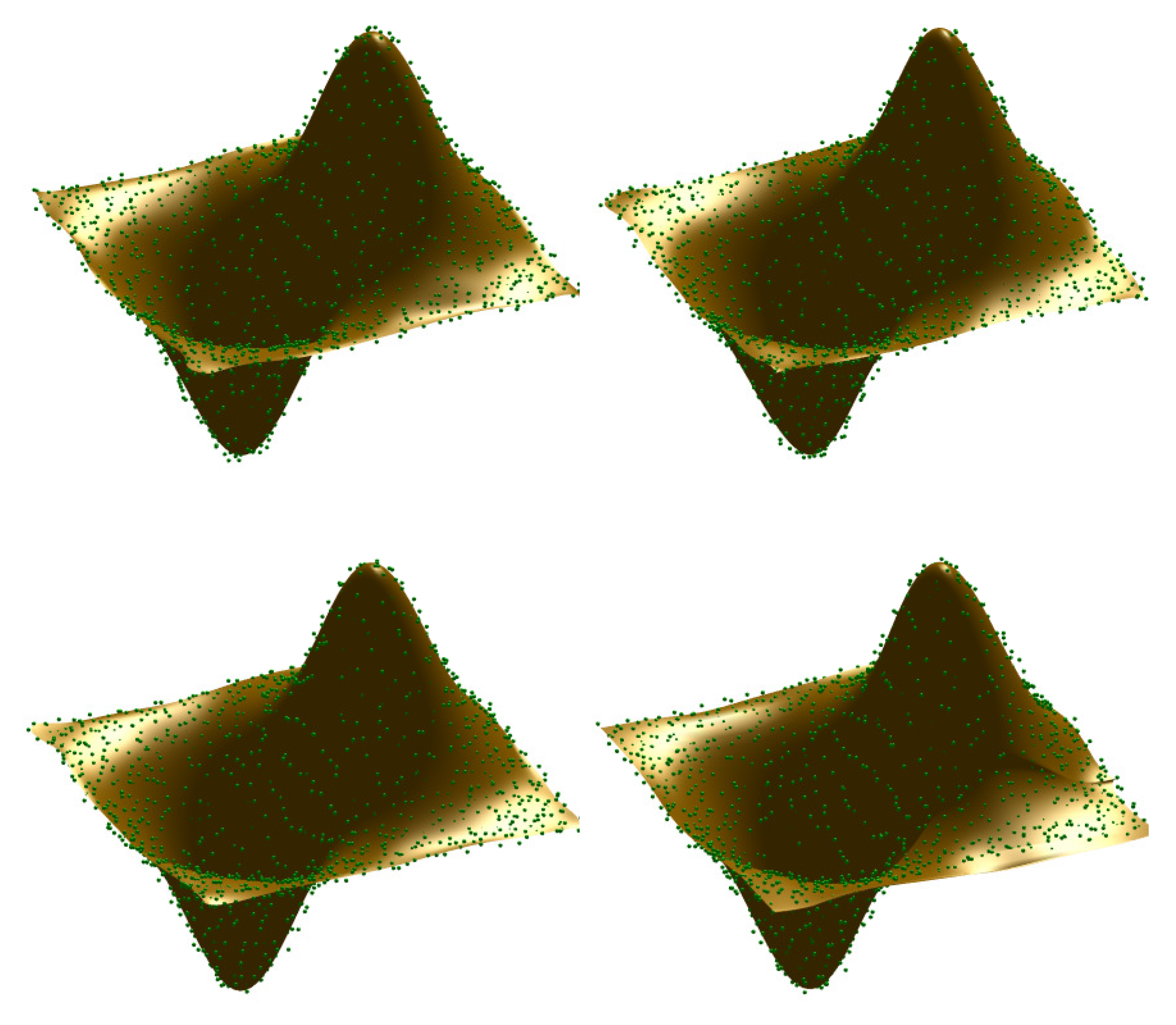
• Our method improves the most classical parameterization methods described in the literature in our comparison. The error rate of the alternative approaches with respect to our method shows that it provides a significant improvement, not just incremental enhancements. This fact is also visible in Figure 7, Figure 8 and Figure 9, where the resulting Bézier surfaces for the uniform, chordal, and centripetal parameterizations, and with our method are displayed for easier visual inspection for the three examples in our benchmark, respectively.
• Among these parametrization methods, the centripetal parameterization yields the closest results to ours in all cases. In fact, it might be a competitive method for some applications, but fails to yield even near-optimal solutions. This fact is clearly noticeable from Table 4 by simple visual inspection of the corresponding numerical values.
• In general, both the uniform and the chordal parameterization yields approximation surfaces of moderate quality. We also remark that the chordal approximation performs even worse than uniform parameterization for Example I while it happens the opposite way for Example III and they perform more or less similarly for Example II. These results are related to the fact that data points for Example I and Example II are noisy but organized, while they are unorganized for Example III. The uniform parameterization does not perform well for such uneven distribution of points.
• The comparison of CSA and its variant ICSA shows that they perform very similarly for the three examples in the benchmark. In fact, the mean value is slightly better for ICSA while the best value is better for CSA for the three examples. This means that the method ICSA tends to have less variation for different executions (as confirmed by the smaller values for the variance and standard deviation than CSA), but CSA is better at approaching to the global minima. However, the differences between both methods are very small and none of them seems to dominate the other for our benchmark.

7.2. Statistical Analysis

It is always advisable to perform some kind of statistical analysis for a more rigorous comparison among different algorithms. It has been pointed out that the parametric tests, albeit widely used in the analysis of experiments, are based on assumptions that are commonly violated in the field of computational intelligence, and, hence, nonparametric tests are recommended instead [47]. According to this remark, we performed a statistical analysis of our results using two popular nonparametric tests for pairwise comparisons: the two-sided Wilcoxon signed rank test (labelled Wilcoxon sign for short in this paper) and the two-sided Wilcoxon rank sum test (labelled Wilcoxon sum here, and that is equivalent to a Mann–Whitney U-test).

The corresponding results of this nonparametric statistical analysis are reported in

Table 5. Pairwise nonparametric statistical tests of the methods in our comparison (in rows) for the three examples in this paper (in columns). Unless otherwise stated, the level of significance for the tests is assumed to be $\alpha =0.05$.

Comparison	Index	Example I	Example II	Example III
CSA vs. Uniform	p-value (Wilcoxon sign):	8.663083 × 10${}^{-8}$	1.572960 × 10${}^{-4}$	7.556929 × 10${}^{-10}$
	signed rank:	1192	1029	1275
	h:	1	1	1
	p-value (Wilcoxon sum):	3.191585 × 10${}^{-7}$	1.115515 × 10${}^{-4}$	7.032679 × 10${}^{-18}$
	rank sum:	3267	3086	3775
	h:	1	1	1
CSA vs. Chordal	p-value (Wilcoxon sign):	8.534226 × 10${}^{-10}$	4.000165 × 10${}^{-5}$	1.110095 × 10${}^{-9}$
	signed rank:	1273	1063	1225
	h:	1	1	1
	p-value (Wilcoxon sum):	8.003963 × 10${}^{-17}$	3.919684 × 10${}^{-5}$	1.032414 × 10${}^{-17}$
	rank sum:	3734	3122	3675
	h:	1	1	1
CSA vs. Centripetal	p-value (Wilcoxon sign):	6.394483 × 10${}^{-6}$	8.626159 × 10${}^{-2}$	1.087244 × 10${}^{-8}$
	signed rank:	1105	460	1269
	h:	1	1 ($\alpha =0.1$)	1
	p-value (Wilcoxon sum):	8.317099 × 10${}^{-6}$	0.148521 × 10${}^{-1}$	1.109774 × 10${}^{-15}$
	rank sum:	3172	2325	3688
	h:	1	1 ($\alpha =0.15$)	1
CSA vs. ICSA	p-value (Wilcoxon sign):	4.784510 × 10${}^{-1}$	8.280511 × 10${}^{-1}$	4.900625 × 10${}^{-1}$
	signed rank:	441	615	709
	h:	0	0	0
	p-value (Wilcoxon sum):	3.883964 × 10${}^{-1}$	p = 7.275182 × 10${}^{-1}$	3.024247 × 10${}^{-1}$
	rank sum:	2125	2475	2675
	h:	0	0	0

. We perform pairwise comparisons of our CSA-based approach with each of the four alternative methods (in rows) for the three examples in the paper (in columns). For each pair, we compute the following parameters (in rows): the p-value, the signed rank, and the value of h for the Wilcoxon sign test, and p-value, the rank sum, and the value of h for the Wilcoxon sum test. For both tests, the value $h=1$ indicates that the null hypothesis of equality of means is rejected for the level of significance $\alpha =0.05$ (the threshold value), while the value $h=0$ indicates a failure to reject the null hypothesis. We also consider higher values for $\alpha$ when necessary for a more accurate analysis of our results.

As shown in Table 5, the p-value of the pairwise comparison between our CSA-based method and the three most classical parameterization methods is very small, ranging from ${10}^{-4}$ to ${10}^{-18}$. In addition, the h index takes the value 1 for all these pairs and all the examples in this paper. These results indicate a significant improvement of our method over these parameterization schemes with a level of significance $\alpha =0.05$. The only exception is given by the centripetal parameterization for the Example II, where the p-values are of order ${10}^{-2}$ and ${10}^{-1}$ for the Wilcoxon sign and the Wilcoxon sum, respectively, leading to a value $h=0$ for $\alpha =0.05$. However, we also obtained $h=1$ for $\alpha =0.1$ and $\alpha =0.15$, respectively. This means that the our method outperforms the centripetal parameterization for such levels of significance.

On the other hand, the pairwise comparison of CSA and ICSA indicates that they perform similarly, as the p-value is always larger than $0.3$ and the h index takes the value $h=0$ for all the examples and both nonparametric tests. From these data, we can conclude that both methods are equivalent and none of them can claim superiority over the other. These results confirm our previous assessment from Table 4 about the comparison between both methods for the problem in this paper.

8. Conclusions

This paper addresses the general problem of global-support free-form parametric surface approximation from clouds of (either organized or scattered) noisy data points for reverse engineering applications. Given a set of measured data points, the approximation is formulated as a nonlinear continuous least-squares optimization problem. Then, a recent metaheuristics called cuckoo search algorithm is applied to compute all relevant free variables of this minimization problem: the data parameters and the surface poles. The method includes the iterative generation of new solutions by using the Lévy flights, a strategy to promote the diversity of solutions and prevent stagnation. A critical advantage of this method is its simplicity: the cuckoo search algorithm requires only two parameters, many fewer than any other metaheuristic approach, so the parameter tuning becomes an easy task. The method is also very simple to understand and easy to implement. The method is very general, in the sense that it can be applied not only to parametric Bézier surfaces, but also to any other global-support free-form parametric surface by simply replacing the Bernstein polynomials by the corresponding basis functions without further modification.

The proposed method has been applied to a benchmark of three illustrative sets of noisy data points corresponding to surfaces exhibiting several challenging features. For instance, they include both organized and unorganized data points (the first two examples and the last one, respectively). They also include several changes of concavity, strong changes of curvature, cusp points and self-intersections. Our experimental results show that the method performs very well for all instances in our benchmark. We also carried out some comparative work with the three most classical mathematical techniques for this problem as well as a recent variant of the cuckoo search algorithm called Improved CSA. Our numerical results and nonparametric statistical tests show that our method improves the accuracy of the results of these three classical methods in all cases. Furthermore, the improvement rate is significant, not merely incremental, as confirmed by the statistical tests. The pairwise comparison between our method and ICSA show that they perform similarly for this problem. This result can be explained by the observation that the performance of the CSA is barely affected by changes of the $p_a$ parameter. In fact, the performance is not affected by choosing a fixed value for $p_a$ or changing it dynamically, provided that those values are taken in a similar region. As a consequence, both CSA and ICSA can be successfully applied to this problem without any statistical advantage over the other. In this case, CSA is recommended because of its simplicity. We can conclude that our method performs very well and can be directly applied to real-world applications for reverse engineering without further pre/post-processing.

The main advantages of our method are its good performance and its simplicity. While the former can also be attained with other methods (such as ICSA, as discussed in Section 7, and possibly others), the latter is a clear advantage with respect to other powerful and popular metaheuristic methods such as genetic algorithms, particle swarm optimization (PSO), and others. In general, such methods depend on several parameters that have to be properly tuned for good performance. In addition, because this choice is problem-dependent, it is typically performed empirically, mostly on a trial-and-error basis. This leads to a cumbersome, time-consuming and error-prone process. In clear contrast, the parameter tuning with CSA is very simple, as our method does depend on only two parameters. Furthermore, the method is very robust against changes of these parameters, meaning that we do not need an optimal tuning for good performance. This does not happen with genetic algorithms, PSO and other methods, whose behavior is strongly affected by the choice of parameter values. Thus, CSA is particularly advantageous for applications where little or no knowledge about the problem to be solved is available.

The main limitations of this method concern the computation times and its inability to ensure that a global optimum is achieved. About the former, the CPU times range from several minutes to a few hours, which can be cumbersome (even unacceptable) for some practical applications. About the latter, this limitation is not exclusive of the CSA, but it applies to all metaheuristic techniques. The field still lacks theoretical studies about the conditions for convergence of the method to global optima. This fact can be a limiting factor for some critical applications, particularly those hazardous where safety is a must.

Our future work includes the extension of this method to more general surfaces. We are particularly interested in the case of rational surfaces, where we have some additional variables that have to be computed as well. Some applications to real-world problems in fields such as CAD/CAM and computer graphics are also part of our plans for future work in the field.

References

1. Patrikalakis, N.M.; Maekawa, T. Shape Interrogation for Computer Aided Design and Manufacturing; Springer: Heidelberg, Germany, 2002. [Google Scholar]
2. Pottmann, H.; Leopoldseder, S.; Hofer, M.; Steiner, T.; Wang, W. Industrial geometry: Recent advances and applications in CAD. Comput. Aided Des. 2005, 37, 751–766. [Google Scholar] [CrossRef]
3. Varady, T.; Martin, R. Reverse Engineering. In Handbook of Computer Aided Geometric Design; Farin, G., Hoschek, J., Kim, M., Eds.; Elsevier Science: Amsterdam, The Netherlands, 2002. [Google Scholar]
4. Dierckx, P. Curve and Surface Fitting with Splines; Oxford University Press: Oxford, UK, 1993. [Google Scholar]
5. Farin, G. Curves and Surfaces for CAGD, 5th ed.; Morgan Kaufmann: San Francisco, CA, USA, 2002. [Google Scholar]
6. Maekawa, T.; Matsumoto, Y.; Namiki, K. Interpolation by geometric algorithm. Comput. Aided Des. 2007, 39, 313–323. [Google Scholar] [CrossRef]
7. Marinov, M.; Kobbelt, L. Optimization methods for scattered data approximation with subdivision surfaces. Graph. Models 2005, 67, 452–473. [Google Scholar] [CrossRef]
8. Sclaroff, S.; Pentland, A. Generalized implicit functions for computer graphics. In Proceedings of the 18th Annual Conference on Computer Graphics and Interactive Techniques, Providence, RI, USA, 27–30 April 1991; Volume 25, pp. 247–250. [Google Scholar]
9. Carr, J.C.; Beatson, R.K.; Cherrie, J.B.; Mitchell, T.J.; Fright, W.R.; McCallum, B.C.; Evans, T.R. Reconstruction and representation of 3D objects with radial basis functions. In Proceedings of the 28th Annual Conference on Computer Graphics and Interactive Techniques, Los Angeles, CA, USA, 12–17 August 2001; pp. 67–76. [Google Scholar]
10. Lim, C.; Turkiyyah, G.; Ganter, M.; Storti, D. Implicit reconstruction of solids from. cloud point sets. In Proceedings of the Third ACM Symposium on Solid Modeling and Applications, Salt Lake City, UT, USA, 17–19 May 1995; pp. 393–402. [Google Scholar]
11. Forsey, D.R.; Bartels, R.H. Surface fitting with hierarchical splines. ACM Trans. Graph. 1995, 14, 134–161. [Google Scholar] [CrossRef]
12. Pratt, V. Direct least-squares fitting of algebraic surfaces. In Proceedings of the 14th Annual Conference on Computer Graphics and Interactive Techniques, Anaheim, California, 27–31 July 1987; Volume 21, pp. 145–152. [Google Scholar]
13. Chih, M. A more accurate second-order polynomial metamodel using a pseudo-random number assignment strategy. J. Oper. Res. Soc. 2013, 64, 198–207. [Google Scholar] [CrossRef]
14. Bajaj, C.; Bernardini, F.; Xu, G. Automatic reconstruction of surfaces and scalar fields from 3D scans. In Proceedings of the 22nd Annual Conference on Computer Graphics and Interactive Techniques, Los Angeles, CA, USA, 6–11 August 1995; pp. 109–118. [Google Scholar]
15. Jones, M.; Chen, M. A new approach to the construction of surfaces from contour data. Comput. Graph. Forum 1994, 13, 75–84. [Google Scholar] [CrossRef]
16. Meyers, D.; Skinnwer, S.; Sloan, K. Surfaces from contours. ACM Trans. Graph. 1992, 11, 228–258. [Google Scholar] [CrossRef]
17. Park, H.; Kim, K. Smooth surface approximation to serial cross-sections. Comput. Aided Des. 1997, 28, 995–1005. [Google Scholar] [CrossRef]
18. Maekawa, I.; Ko, K. Surface construction by fitting unorganized curves. Graph. Models 2002, 64, 316–332. [Google Scholar] [CrossRef]
19. Echevarría, G.; Iglesias, A.; Gálvez, A. Extending neural networks for B-spline surface reconstruction. Lect. Notes Comput. Sci. 2002, 2330, 305–314. [Google Scholar]
20. Gu, P.; Yan, X. Neural network approach to the reconstruction of free-form surfaces for reverse engineering. Comput. Aided Des. 1995, 27, 59–64. [Google Scholar] [CrossRef]
21. Ma, W.Y.; Kruth, J.P. Parameterization of randomly measured points for least squares fitting of B-spline curves and surfaces. Comput. Aided Des. 1995, 27, 663–675. [Google Scholar] [CrossRef]
22. Eck, M.; Hoppe, H. Automatic reconstruction of B-Spline surfaces of arbitrary topological type. In Proceedings of the 23rd Annual Conference on Computer Graphics and Interactive Techniques, New Orleans, LA, USA, 4–9 August 1996; pp. 325–334. [Google Scholar]
23. Piegl, L.; Tiller, W. The NURBS Book; Springer: Berlin/Heidelberg, Germany, 1997. [Google Scholar]
24. Hoffmann, M. Numerical control of Kohonen neural network for scattered data approximation. Numer. Algorithms 2005, 39, 175–186. [Google Scholar] [CrossRef]
25. Knopf, G.K.; Kofman, J. Adaptive reconstruction of free-form surfaces using Bernstein basis function networks. Eng. Appl. Artif. Intell. 2001, 14, 577–588. [Google Scholar] [CrossRef]
26. Barhak, J.; Fischer, A. Parameterization and reconstruction from 3D scattered points based on neural network and PDE techniques. IEEE Trans. Vis. Comput. Graph. 2001, 7, 1–16. [Google Scholar] [CrossRef]
27. Liu, X.; Tang, M.; Frazer, J.H. Shape reconstruction by genetic algorithms and artificial neural networks. Eng. Comput. 2003, 20, 129–151. [Google Scholar] [Green Version]
28. Gálvez, A.; Iglesias, A.; Cobo, A.; Puig-Pey, J.; Espinola, J. Bézier curve and surface fitting of 3D point clouds through genetic algorithms, functional networks and least-squares approximation. Lect. Notes Comput. Sci. 2007, 4706, 680–693. [Google Scholar]
29. Iglesias, A.; Echevarría, G.; Gálvez, A. Functional networks for B-spline surface reconstruction. Future Gener. Comput. Syst. 2004, 20, 1337–1353. [Google Scholar] [CrossRef]
30. Iglesias, A.; Gálvez, A. Hybrid functional-neural approach for surface reconstruction. Math. Probl. Eng. 2014. [Google Scholar] [CrossRef]
31. Yang, X.-S. Nature-Inspired Metaheuristic Algorithms, 2nd. ed.; Luniver Press: Frome, UK, 2010. [Google Scholar]
32. Yang, X.-S. Engineering Optimization: An Introduction with Metaheuristic Applications; John Wiley & Sons: Hoboken, NJ, USA, 2010. [Google Scholar]
33. Gálvez, A.; Iglesias, A. Efficient particle swarm optimization approach for data fitting with free knot B-splines. Comput. Aided Des. 2011, 43, 1683–1692. [Google Scholar] [CrossRef]
34. Yoshimoto, F.; Harada, T.; Yoshimoto, Y. Data fitting with a spline using a real-coded algorithm. Comput. Aided Des. 2003, 35, 751–760. [Google Scholar] [CrossRef]
35. Gálvez, A.; Iglesias, A.; Avila, A.; Otero, C.; Arias, R.; Manchado, C. Elitist clonal selection algorithm for optimal choice of free knots in B-spline data fitting. Appl. Soft Comput. 2015, 26, 90–106. [Google Scholar] [CrossRef]
36. Ulker, E.; Arslan, A. Automatic knot adjustment using an artificial immune system for B-spline curve approximation. Inf. Sci. 2009, 179, 1483–1494. [Google Scholar] [CrossRef]
37. Zhao, X.; Zhang, C.; Yang, B.; Li, P. Adaptive knot adjustment using a GMM-based continuous optimization algorithm in B-spline curve approximation. Comput. Aided Des. 2011, 43, 598–604. [Google Scholar] [CrossRef]
38. Gálvez, A.; Iglesias, A. A new iterative mutually-coupled hybrid GA-PSO approach for curve fitting in manufacturing. Appl. Soft Comput. 2013, 13, 1491–1504. [Google Scholar] [CrossRef]
39. Gálvez, A.; Iglesias, A. Particle swarm optimization for non-uniform rational B-spline surface reconstruction from clouds of 3D data points. Inf. Sci. 2012, 192, 174–192. [Google Scholar] [CrossRef]
40. Gálvez, A.; Iglesias, A.; Puig-Pey, J. Iterative two-step genetic-algorithm method for efficient polynomial B-spline surface reconstruction. Inf. Sci. 2012, 182, 56–76. [Google Scholar] [CrossRef]
41. Garcia-Capulin, C.H.; Cuevas, F.J.; Trejo-Caballero, G.; Rostro-Gonzalez, H. Hierarchical genetic algorithm for B-spline surface approximation of smooth explicit data. Math. Probl. Eng. 2014, 2014. [Google Scholar] [CrossRef]
42. Zhao, X.; Zhang, C.; Xu, L.; Yang, B.; Feng, Z. IGA-based point cloud fitting using B-spline surfaces for reverse engineering. Inf. Sci. 2013, 245, 276–289. [Google Scholar] [CrossRef]
43. Yang, X.S.; Deb, S. Cuckoo search via Lévy flights. In Proceedings of the 2009 World Congress on Nature & Biologically Inspired Computing, Coimbatore, India, 9–11 December 2009; pp. 210–214. [Google Scholar]
44. Yang, X.S.; Deb, S. Engineering optimization by cuckoo search. Int. J. Math. Model. Numer. Optim. 2010, 1, 330–343. [Google Scholar]
45. MatlabCentral Repository. Available online: http://www.mathworks.com/matlabcentral/fileexchange/29809-cuckoo-search-cs-algorithm (accessed on 25 December 2017).
46. Valian, E.; Tavakoli, S.; Mohanna, S.; Hahgi, A. Improved cuckoo search for reliability optimization problems. Comput. Ind. Eng. 2013, 64, 459–468. [Google Scholar] [CrossRef]
47. Derac, J.; García, S.; Molina, D.; Herrera, F. A practical tutorial on the use of nonparametric statistical tests as a methodology for comparing evolutionary and swarm intelligence algorithms. Swarm Evolut. Comput. 2011, 1, 3–18. [Google Scholar] [CrossRef]
Figure 1. Application of our method to Example I: (top) given cloud of noisy data points; (bottom) noisy data points and best approximating Bézier surface.
Symmetry 10 00058 g001
Figure 2. Convergence diagram for Example I.
Symmetry 10 00058 g002
Figure 3. Application of our method to Example II: (top) given cloud of noisy data points; (bottom) noisy data points and best approximating Bézier surface.
Symmetry 10 00058 g003
Figure 4. Convergence diagram for Example II.
Symmetry 10 00058 g004
Figure 5. Application of our method to Example III: (top) given cloud of noisy data points; (bottom) noisy data points and best approximating Bézier surface.
Symmetry 10 00058 g005
Figure 6. Convergence diagram for Example III.
Symmetry 10 00058 g006
Figure 7. Visual comparison of different methods for Example I: (top-left) uniform parameterization; (top-right) chordal parameterization; (bottom-left) centripetal parameterization; (bottom-right) our method.
Symmetry 10 00058 g007
Figure 8. Visual comparison of different methods for Example II: (top-left) uniform parameterization; (top-right) chordal parameterization; (bottom-left) centripetal parameterization; (bottom-right) our method.
Symmetry 10 00058 g008
Figure 9. Visual comparison of different methods for Example III: (top-left) uniform parameterization; (top-right) chordal parameterization; (bottom-left) centripetal parameterization; (bottom-right) our method.
Symmetry 10 00058 g009