The Impact of the Anisotropy of the Media between Parallel Plates on the Casimir Force

1
Hubei Collaborative Innovation Center for High-Efficiency Utilization of Solar Energy, Hubei University of Technology, Wuhan 430068, China
2
School of Science, Hubei University of Technology, Wuhan 430068, China
3
MOE Key Laboratory of Fundamental Physical Quantities Measurement, Hubei Key Laboratory of Gravitation and Quantum Physics, School of Physics, Huazhong University of Science and Technology, Wuhan 430074, China
*
Authors to whom correspondence should be addressed.
Symmetry 2018, 10(3), 61; https://doi.org/10.3390/sym10030061
Submission received: 30 December 2017
/
Revised: 9 February 2018
/
Accepted: 2 March 2018
/
Published: 7 March 2018
(This article belongs to the Special Issue Casimir Physics and Applications)
Abstract
:Quantum fluctuations of the electromagnetic field give rise to the force between parallel plates: the Casimir force. We theoretically calculate the Casimir force between two parallel isotropic plates when the space between the plates is filled with anisotropic material. Our result shows that the Casimir force, especially in the direction of the force, can be significantly affected by the anisotropy of the intervening material. We also discuss the combined influence of dispersion and anisotropy, and analyze the impact of the external electric filed on the Casimir force by affecting the anisotropy of the intervening material by Kerr electro-optical effect.
1. Introduction
The Casimir effect, which is a macroscopic quantum effect arising from the quantum fluctuations of the electromagnetic field is one of the most remarkable findings of quantum field theory [1,2,3,4,5,6]. Over past years, the Casimir effect has drawn a lot of experimental and theoretical attention, as it plays a significant role in various fields of physics [4,5,6].
Lifshitz’s original theory for the force between dielectric plates is based on isotropic dielectrics, and is not applicable to anisotropic materials. However, if the anisotropy of the plates is considered, we can see some new features of the Casimir effect, like Casimir torque. Parsegian calculated the van der Waals interaction energy between two uniaxial bodies in the nonretarded limit [7]. Barash calculated the torque of van der Waals forces between two anisotropic thick plates [8]. Based on previous works, Munday et al. calculated the Casimir torque between parallel anisotropic plates immersed in liquid, and their recent works showed that the retardation and the intervening dielectric could enhance this torque [9,10]. As a supplementary work, Shao et al. gave the analytical expression of the Casimir torque between two birefringent plates with static permittivity [11]. In one of our works, we calculated the Casimir torque between parallel birefringent plates with frequency dependent magnetic permeabilities, and showed that the magnetic properties of the plates could significantly affect the torque [12]. Anisotropy does not only affect the Casimir torque, but it also affects the Casimir force directly. Romanowsky found that the orientation of the optical axis of highly anisotropic materials could significantly affect the Casimir force [13]. The direction of the Casimir force could also be affected by the anisotropy. Shao et al. gave the analytical result of the repulsive Casimir force between two uniaxial plates with static permittivity and permeability [14]. In one of our works, the Casimir force between anisotropic metamaterial plates was calculated [15], and the result showed that the direction of the force depended on the anisotropy in some distance ranges. Parashar and his colleagues calculated the Casimir force between two parallel semitransparent δ-function plates and between two parallel anisotropic dielectric slabs [16]. Somers and Munday found that, for particular orientations of optical axes, the Casimir force can be repulsive, even when the two anisotropic slabs are identical [17]. In recent years, scientists have started to investigate the interaction between anisotropic particles and a surface [16,18,19].
Most of the previous works [9,10,11,12,13,14,15,16,17,18,19] only focused on the anisotropy of the plates and assumed that the space between the two plates was a vacuum or was filled with isotropic materials. However, in fact, this region could also be anisotropic. Some liquid, like nitrobenzene, can be anisotropic under special circumstances. Moreover, in biology, liquid films between the two biomembranes are often anisotropic. Thus, taking the anisotropy of the intervening media into account should prove both more interesting and closer to reality. Are there any new phenomena if the gap between the two plates is filled with anisotropic media? This is an interesting question. To find answers to this question, Parsegian first calculated the van der Waals interaction energy between two uniaxial slabs acting across a gap that is filled with a third anisotropic material, and the result was limited in the nonretarded case [7]. Kornilovitch investigated the impact of angle between the optical axis and the surface normal on the Van der Waals interaction between parallel slabs in uniaxial media, and their result was also in the nonretarded limit [20]. When compared with attractive Casimir force, repulsive force is more interesting to researchers [2,3,4,5,6,9,11,14,15,17]. According to Lifshitz’s theory, the repulsive Casimir force arises between two materials that are separated by a third isotropic material whose dielectric permittivity is intermediate to the other two materials [2,3]. However, if the intervening media is anisotropic, ε3 will have different values in different directions. Accordingly, this makes the condition for repulsive force more complicated. One of our recent works shows that it is still possible to have repulsive force in this case and that the force can be significantly affected by the anisotropy of the media between the plates [21]. As we know liquid like nitrobenzene can be anisotropic under an external field [22,23,24]. This means that the external field can affect the Casimir force by affecting the anisotropy of the intervening media. This is important for both theoretical and experimental investigations on the Casimir effect. In order to supplement our previous work [18], in this paper, we calculate the fully relativistic Casimir force between two isotropic plates separated by a gap filled with a third uniaxial material, and then analyze the exact impact of the anisotropy of the intervening media and dispersion on the Casimir force. Furthermore, we discuss the influence of the external electric field on the Casimir effect by affecting the anisotropy of the intervening media though the Kerr electro-optical effect.
2. Calculation of the Casimir Force between Parallel Slabs Separated by Uniaxial Material
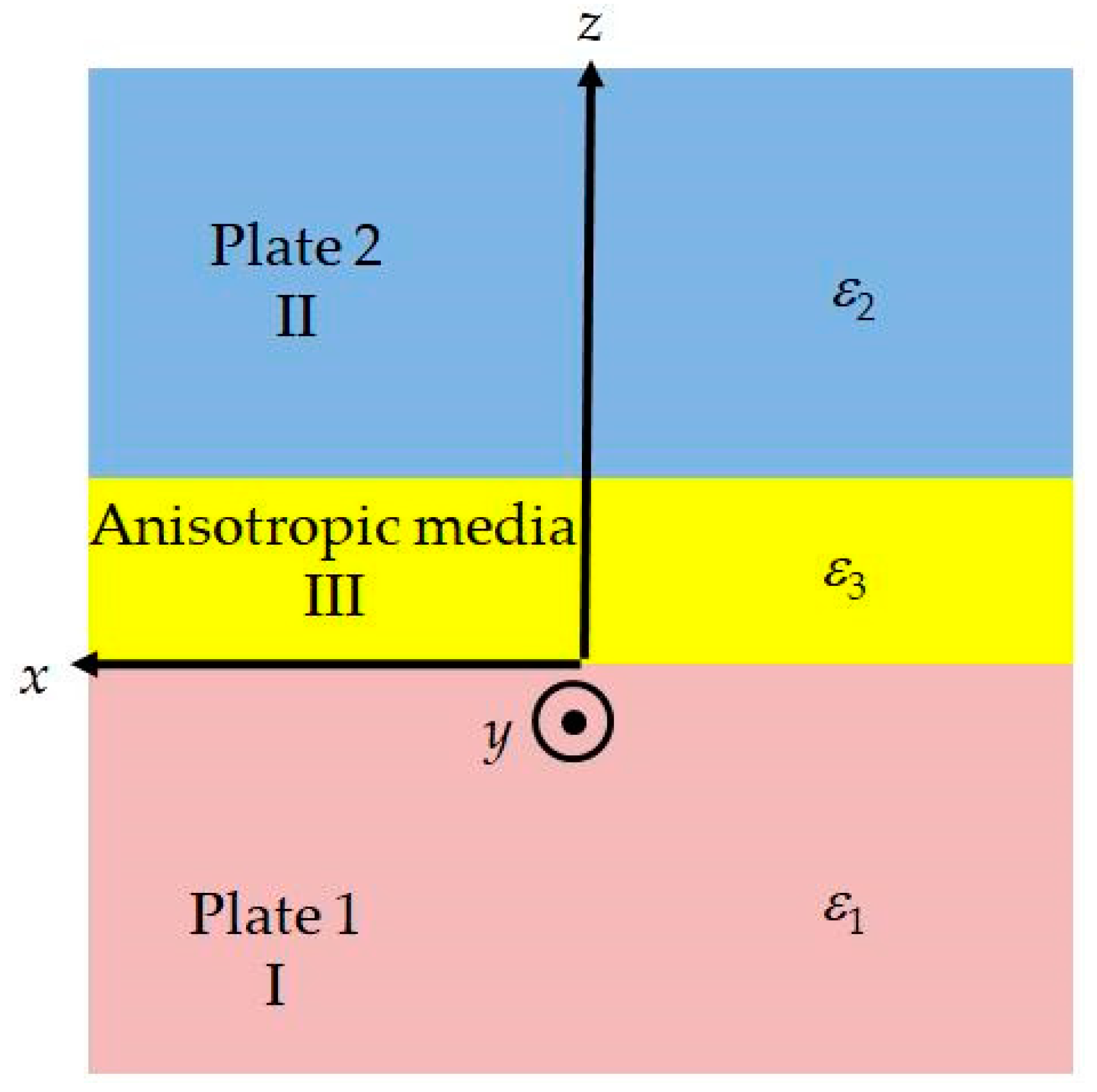
In this section, we will give a detailed calculation of the Casimir force between two parallel isotropic slabs separated by uniaxial material. We consider two parallel plates (with diameter D and thickness d) made of isotropic materials, with the distance between them being a (as shown in Figure 1). The gap between the two plates is filled with uniaxial material. Both the plates and the material between them are assumed to be nonmagnetic in this paper. We consider the case that the optical axis of the anisotropic media is perpendicular to the surfaces of the plates. We let the x-y plane be parallel to the surfaces of the plates. Therefore, the optical axis of the intervening anisotropic media is in z direction. In view of D >> a and d >> a, the system may be considered to be two parallel semi-infinite plates separated by anisotropic uniaxial material with an optical axis in z direction as shown in Figure 2. Therefore, the space could be considered to be divided into three regions (I, II, III). The dielectric properties of each region can be described by corresponding relative permittivities.
The relative dielectric pemittivities of the plates and the anisotropic media between them can be expressed by following matrices [11,12,14,17,21,24].
where the subscripts z and x indicate the components of the permittivity tensors parallel and perpendicular to the optical axis, respectively.
Due to the fact that all of the regions in Figure 2 are considered to be homogenous, the electric and magnetic fields with the surface mode q can be written as [21,25].
where N is the normalization factor. The parameters aq and in (4) and (5) are the usual creation and annihilation operators, respectively. k = (kx, ky, kz) is the wave vector. We can choose ky = 0 without loss of generality, and we can have k = (kx, 0, kz) = K0 (α, 0, γ), with K0 = ωc−1. In order to determine the mode of the electric and magnetic field eq and hq with frequency ω, we can use the classical Maxwell equations without sources.
where εi (i = 1, 2, 3) is the dielectric permittivity in region I, II, and III, which could be expressed by Equations (1)–(3). The solution of the electromagnetic fields can be expressed in the plane wave form as:
Here, ex, ey, and ez indicate the elements of the electric field (E) polarization vectors, and bx, by, and bz indicate the elements of the magnetic field (B) polarization vectors. As all of the materials that are considered in this paper are assumed to be nonmagnetic, we can have B = μ0H.
Substituting (1) and (8) into (4) and (5), we can obtain the eigenequations of the transverse elements of the electric and magnetic field polarization vectors ex, ey bx, and by in region: I
Moreover, the four eigenvectors and their corresponding eigenvalues can be expressed in the matrix form:
with (t1)2 = α2 − ε1. These four eigenvalues correspond to four independent mode solutions whose linear superposition should be the general solution of the electromagnetic field. Further, the superposition coefficients should be the amplitudes of each mode. Therefore, the transverse elements of the electromagnetic field modes in (4) and (5) in region I can be expressed as:
Similarly, in region II, the transverse elements of the electromagnetic field modes in (4) and (5) can be expressed as:
with:
and:
where (t2)2 = α2 − ε2.
In region III, where it is anisotropic, the case is slightly different. However, the method for calculation is similar. Therefore, we can have the transverse elements of the electromagnetic field modes in (4) and (5) in region III:
with:
and:
where (t3x)2 = α2 − ε3x and (t3z)2 = (α2 − ε3z)(ε3x/ε3z).
For the requirement that the surface modes should be exponentially decaying when z > a and z < 0, we have AI,3 = AI,4 = AII,1 = AII,2 = 0. As the boundary conditions require the transverse elements of the electromagnetic field to be continuous at z = a and z = 0, we can get a set of eight linear homogeneous equations that are relating the unknown coefficients AI,1, AI,2, AII,3, AII,4, AIII,1, AIII,2, AIII,3, and AIII,4. It has nontrivial solutions if the determinant of its coefficients is equal to zero, which is, accordingly, the equation to determine the proper frequency ω of the modes. This equation can be expressed as:
The subscripts ⊥ and || indicate the modes with the polarization of the field perpendicular and parallel to the plane formed by k|| = (kx, ky) and z (according to previous assumption, this plane is x-z plane), respectively. We introduce δ = (ε3z/ε3x) − 1 to express the degree of anisotropy of the intervening material between the plates, and δ = 0 refers to isotropic media. The detailed expression of the functions D1 and D2 can be found in Appendix A, and the functions G1 and G2 can be expressed as (ω = iξ),
where the notations p2 = 1 − α2/ε3x, (s1)2 = −(t1)2/ε3x, and (s2)2 = −(t2)2/ε3x have been introduced.
According to the method that used in [4,11,14,21], the Casimir interaction energy at zero temperature can be expressed as (the detailed mathematical derivation of (22) can be found in Appendix A)
The Casimir force between the plates per unit area should be:
It is clear that the Casimir force F(a) in (23) depends on δ, the degree of anisotropy of the material between the plate. This means the anisotropy of the intervening material does affect the Casimir force. However, one should also notice that G1 does not depend on δ, which means that the anisotropy affects the Casimir force only though the second term in the bracket in (23). When δ = 0, (23) becomes:
which is coincident with Lifshitz’s formula for isotropic materials (Equation (4.14) in [3]).
If we assume that the separation between the plates a is greater than the characteristic absorption wavelength of the materials, we could replace the permittivities ε3x, ε3z, ε1, and ε2 with their values at ξ = 0 (ε3x0, ε3z0, ε10, and ε20) [3]. Also, (23) can be written with considerable accuracy in the form:
with:
3. The Impact of the Anisotropy of the Intervening Material between the Plates on Casimir Force
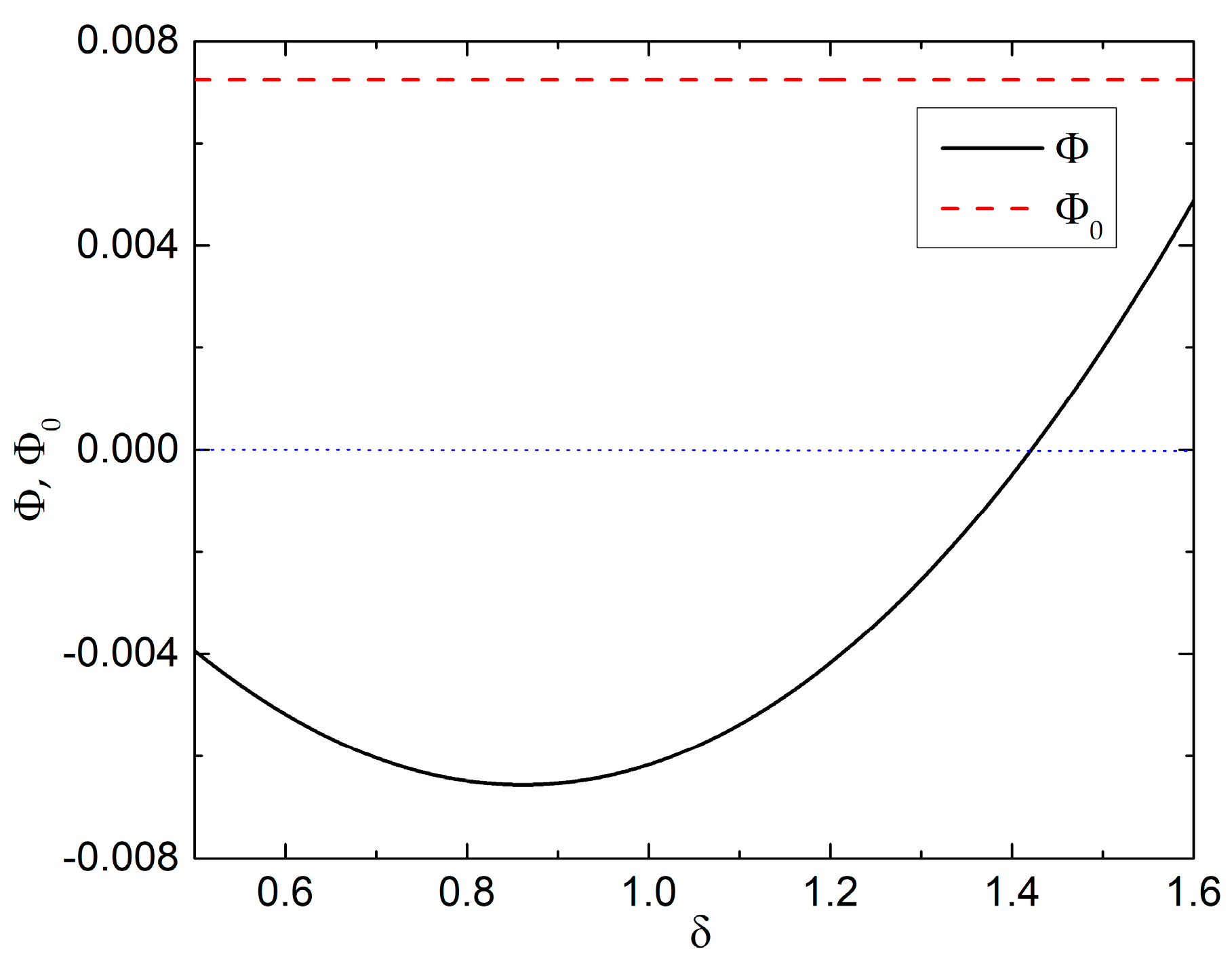
In this section, we will analyze the impact of the anisotropy of the intervening material between the plates on Casimir force. According to (25) and (26), the function Φ is proportional to the magnitude of the force and can reflect the direction of the force. The positive Φ indicates that the force is attractive, while the negative Φ indicates that the force is repulsive. As we are mainly interested in the impact of the anisotropy of the intervening media on the Casimir force, especially the direction of the force, we simply need to focus on the sign of the function Φ.
For convenience, we can assume that ε10 > ε20. We need to emphasize that the case in which ε10 > ε3x0 > ε20 and ε10 > ε3z0 > ε20 are satisfied at the same time is not within our interests. This is because in this case, all the possible values of ε30 are greater than ε10 and smaller than ε20, and this will make the force repulsive, which is almost the same as Lifshitz’s result [3]. For the same reason, we also do not have interests in the case when both ε3x0 and ε3z0 are greater than ε10 or when both ε3x0 and ε3z0 are smaller than ε20. Therefore, we only need to focus on two cases: 1. only one of ε3x0 and ε3z0 is between ε10 and ε20; and, 2. one of ε3x0 and ε3z0 is smaller than ε20, while the other one is greater than ε10.
For case 1, we let ε10 > ε3x0 > ε20 > ε3z0 (or ε3z0 > ε10 > ε3x0 > ε20). The value of Φ for different δ, the degree of anisotropy, is shown in Figure 3. The positive Φ indicates that the force is attractive, while the negative Φ indicates that the force is repulsive. In Figure 3a, where ε10 > ε3x0 > ε20 > ε3z0, we can see that the Casimir force is attractive at beginning and the magnitude decreases as the degree of anisotropy δ changes. Finally, it switches into repulsive. In Figure 3b, where ε3z0 > ε10 > ε3x0 > ε20, the Casimir force is repulsive at beginning and then switches into attractive as the degree of anisotropy δ changes. Therefore, we can conclude that the magnitude, as well as the direction, of the Casimir force could be significantly affected by the anisotropy of the intervening material in case 1. For a case where ε3z0 is between ε10 and ε20, but ε3x0 is not, the result is similar.
For case 2, let us consider ε3z0 > ε10 > ε20 > ε3x0. The value of Φ for different δ, the degree of anisotropy, is shown in Figure 4. In Figure 4, we can see that the Casimir force is repulsive at the very beginning and increases as δ increases. Then, as δ increases, the repulsive force starts to decrease, before finally switching into attractive. Therefore, in this case, still, the magnitude as well as the direction of the Casimir force could be significantly affected by the anisotropy of the intervening material.
In our previous work [21], we only roughly divided the force into two parts, which, in fact, is not the best way to analyze the impact of the anisotropy. In order to see it more clearly, in this paper, we expand the function Φ about δ to the first order:
with:
When δ = 0, when substituting (28) and (29) into (25), we can recover Lifshitz’s result for isotropic materials in the same limiting case (Equation (4.20) in [3]).
In (28), Φ0 represents the contribution of isotropy to the total force, while δΦδ represents the contribution of anisotropy. As Φ0 does not depend on δ, it will always be the same value and sign when δ changes. Therefore, the changes of the magnitude and direction of the Casmir force are caused by δΦδ, which depends on the anisotropy of the intervening material. In case 1, Φ0 is always negative and produces a repulsive force. In Figure 3a,b, it is clear that when the absolute value of δ increases, the repulsive force becomes smaller and finally changes into an attractive force. This means that the anisotropy can produce an attractive force against the repulsive force that is produced by Φ0, the isotropic term. When the contribution from anisotropy is greater than the contribution from isotropy, the force switches its direction. In case 2, Φ0 is always positive and produces an attractive force. However, the total force is not always attractive, because the anisotropy can produce a repulsive force against the attractive force produced by Φ0, the isotropic term. One should notice that the curve in Figure 3a represents a good linear relationship, while the curves in Figure 3b and Figure 4 do not represent a linear relationship. This is because the expansion in (28)–(30) is only valid for small δ, but the values of δ are not so small in Figure 3b and Figure 4. The higher order terms of δ produce the nonlinear relationship between Φ and δ. However, in general, we can draw the conclusion that, in both case 1 and case 2, if the isotropy of the material between the plates contributes a force in a certain direction, the anisotropy could produce a force in the opposite direction. The direction of the Casimir force depends on which one has greater magnitude, which reflects the competition between the contribution from anisotropy and isotropy. The change in the direction of the Casimir force is caused by the change of the degree of anisotropy of the material between the plates in this limiting case. This confirms our conclusion in [21], where we roughly divided the force into two parts.
4. The Impact of the Dispersion
One may notice that, in the previous section, the force seemed to switch direction at the same δ for all of the separations if the materials are specified. This is because, in previous sections, we want to focus on the influence of anisotropy of the intervening material only, and we ignore the dispersion, which makes the function Φ independent of a and ξ. However, for real material, the case should not be always like this, and it is necessary to consider the effects of dispersion. Therefore, in this section, we will discuss the combined influence of dispersion and anisotropy of the intervening material between the plates.
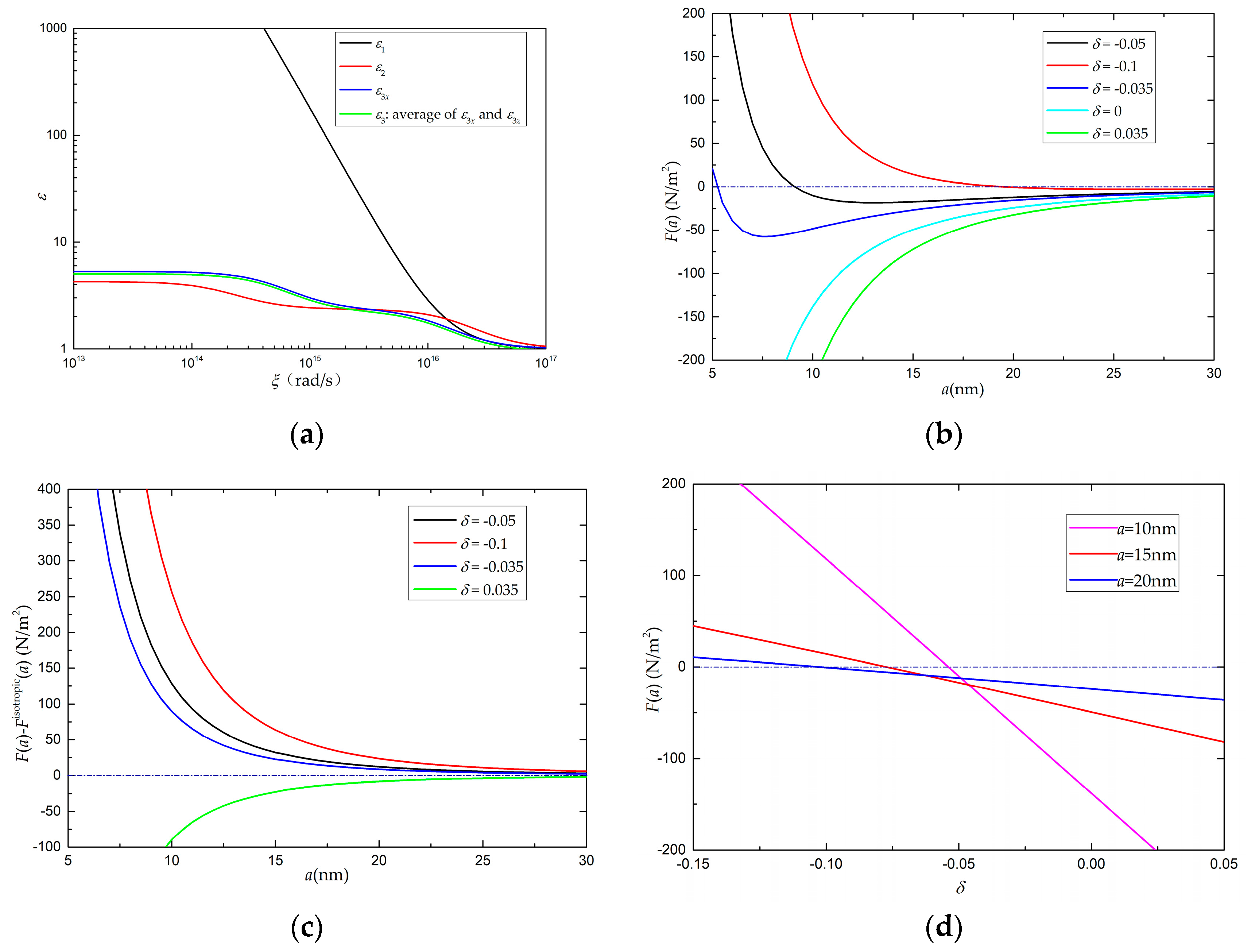
In this section, we consider that he permittivities are frequency dependent, as shown in Figure 5a. ε3 is the average value of ε3z and ε3x. The models of the dispersion relations and the parameters used are described in Appendix B. The Casimir forces at different separations for different values of δ are calculated with (23) and the result is shown in Figure 5b. The positive value indicates that the force is attractive, while the negative value indicates that the force is repulsive. The force is repulsive in wide distance range, and can be attractive only at very small separations. This behavior can be explained by the inequality between ε1, ε2 and ε3. ε3 is the average value of ε3z and ε3x. The inequality ε1 > ε3 > ε2 is satisfied for the frequencies lower than ~2 × 10¹⁵ rad/s, and the modes with these low frequencies will contribute to a repulsive force. For the frequencies that are higher than ~2 × 10¹⁵ rad/s, the inequality ε1 > ε3 > ε2 is no longer valid, and the modes with these high frequencies will contribute to an attractive force. The direction of the total force depends on which contribution is greater. At small separation, the contribution from high frequency modes is dominant and the force is attractive; while at large separation, the contribution from low frequency modes is dominant and the force switches into repulsive.
The result above is similar to the result in [9]. However, it remains different and interesting. One can notice that without anisotropy the force is always repulsive for separations that are greater than a few nanometers. However, if anisotropy of the intervening media is considered, the force can be attractive even at a separation greater than 10 nanometers. When δ is negative, the greater the value of δ is, the greater the distance range we have for attractive force we have. However, positive δ cannot help to produce attractive force at a distance greater than few nanometers. This can also be explained by the inequality between ε1, ε2 and ε3. The negative δ will make ε3, the average value of ε3z and ε3x, smaller, and the inequality ε1 > ε3 > ε2 will invalidate at even lower frequency. That is why negative δ can help to produce an attractive force.
We can use the difference between F(a) in (23) and Fisotropic(a) to express the impact of anisotropy of the intervening media. As shown in Figure 5c, at the separation greater than few nanometers, negative δ always produces an attractive force, which is coincident with the result in the paragraph above. One may also notice that ε1 is much greater tha n ε2 and ε3 in wide frequency range. Therefore, for small positive δ, it is not possible to make ε3, the average value of ε3z and ε3x, go beyond ε1 at lower frequency. That is why the impact of positive δ is always negative in Figure 5c.
Figure 5d shows that when dispersion is taken into account, the anisotropy can also affect the amplitude and direction significantly. When δ is negative and with a relative large magnitude, the force is attractive. As the magnitude of δ decreases and changes into positive, the force switches into repulsive. We can also find in Figure 5d, that for different separations, the direction of the force reverses at different values of δ, which is different from the result in Section 3, where the static permittivities are used. This means the anisotropy of the intervening material can affect the direction of the Casimir force, but at which separation and which δ the force switches its direction are affected by dispersion. This is the combined influence of dispersion and anisotropy of the material between the plates.
5. The Impact of the External Electric Field on the Casimir Force
When an external electric field is applied across some sample (especially for liquid like nitrotoluene or nitrobenzene), the sample becomes birefringent, which is usually known as Kerr electro-optical effect [22,23]. Therefore, the external electric field can affect both the amplitude and direction of the Casimir force by affecting the degree of anisotropy of the intervening material. If the material between the plates is isotropic and a DC electric field Eext is applied across the material in z direction, then the intervening material will become birefringent, and the relationship between permittivity in z direction and x direction should be: [24]
where ak is associated with the property of the material. Here, we only consider the Kerr electro-optical effect for the material between the plates and do not consider that for the plates, since this effect in solid is often not as strong as that in liquid. As we have introduced δ = (ε3z/ε3x) − 1 to express the degree of anisotropy of the intervening material, we can have:
In experiments and applications about the Casimir force, the electric field is usually reduced to small level. Therefore, anisotropy caused by the electric field will be also small, and the expansion Equation (28) is valid. Substituting (32) into (28), we have:
which means the impact of external electric field on the Casimir force is proportional to the square of the field (we only consider the influence of external electric field by affecting the anisotropy of intervening material). If dispersion is included, one can substitute (32) into (23). This effect will not affect the result of current experiments measuring Casimir force. This is because most of the experiments take place in vacuum and the electric force that is caused by the external electric field could be much greater than this effect. For the same reason, it is also very difficult to observe this effect experimentally.
6. Conclusions
We calculate the fully relativistic Casimir force between two isotropic plates separated by a gap filled with a third anisotropic media. Further, we give the exact result for the impact of the anisotropy of the intervening material on Casimir force. Our result shows that the anisotropy of the intervening material can significantly affect both the magnitude and direction of Casimir force. If the isotropy of the intervening material contributes a force in a certain direction, the anisotropy can contribute a force in opposite direction. The direction of total Casimir force depends on which one has a greater contribution. The change in the direction of the Casimir force is totally caused by the change of the degree of anisotropy of the intervening material when dispersion is ignored. When dispersion is taken into account, the degree of anisotropy of the intervening can still change the direction of the force, but at which distance and what value of the degree of anisotropy the direction changes are determined by dispersion. The external electric field can affect both the amplitude and direction of Casimir force by affecting the anisotropy of the intervening material. This influence is proportional to the square of the strength of external electric field. This effect would not have much influence on current experiments.
Acknowledgments
This work was partially supported by the National Natural Science Foundation of China (Grant No. 11605050, Grant No. 91636221, and Grant No. 11604089). The authors owe all the former works on the Casimir effect, especially [16], for the inspiration for this article.
Author Contributions
All the authors have participated in the research for this paper.
Conflicts of Interest
The authors declare no conflict of interest.
Appendix A
In this section we will give the detailed derivation of Equation (22). From the equation of determinant of coefficients equaling zero that mentioned in Section 2, we can have
where:
and:
The expressions of functions G1 and G2 can be found in (20) and (21) and are transformed into another form with the relations mentioned in Section 2.
The Casimir interaction energy per unit area is
The summation over ω can be calculated with the help of argument theorem, which has been applied in [4,11,14,21],
where C+ indicates a semicircle with infinite radius in the right one-half of the complex plane whose center is the origin. As the function ∆1 and ∆2 are analytic and have no poles along the closed path in (A7) and (A8), argument theorem is capable here. If we assume that along any radial direction in complex plane we can have:
the integration along C+ is infinite and independent of the separation a. To remove this divergence, we can subtract the energy when a→∞ from U(a) and get a renormalized physical Casimir interaction energy per unit area:
and the divergence can be canceled.
According to (A2)–(A5), we can have:
With the help of (A7) and (A8), we can have:
and:
Substitute (A11) and (A12) into (A8) and introduce ω = iξ, we can get (22), with the help of the relations p2 = 1 − α2/ε3x, (s1)2 = −(t1)2/ε3x, and (s2)2 = −(t2)2/ε3x.
Appendix B
In this section, we will describe the models of dispersion relation and the parameters used in the calculations in Section 4.
For plate 1 (ε1), we use the Drude model:
For plate 2 (ε2) and the intervening material between the plates (ε3x), we use the following model:
References
- Casimir, H.B.G. On the Attraction between Two Perfectly Conducting Plates. Proc. Kon. Ned. Akad. Wet. 1948, 51, 793–795. [Google Scholar]
- Lifshitz, E.M. The Theory of Molecular Attractive Forces between Solids. Sov. Phys. JETP 1956, 2, 73–83. [Google Scholar]
- Dzyaloshinskii, I.E.; Lifshitz, E.M.; Pitaevskii, L.P. The General Theory of van der Waals Forces. Adv. Phys. 1961, 10, 165–209. [Google Scholar] [CrossRef]
- Bordag, A.; Mohideen, U.; Mostepanenko, V.M. New developments in the Casimir effect. Phys. Rep. 2001, 353, 1–205. [Google Scholar] [CrossRef]
- Milton, K.A. The Casimir Effect: Physical Manifestations of Zero-Point Energy; World Scientific: Singapore, 2001; ISBN 978-981-02-4397-5. [Google Scholar]
- Klimchitskaya, G.L.; Mohideen, U.; Mostepanenko, V.M. The Casimir force between real materials: Experiment and theory. Rev. Mod. Phys. 2009, 81, 1827. [Google Scholar] [CrossRef]
- Parsegian, V.A.; Weiss, G.H. Dielectric Anisotropy and the van der Waals Interaction between Bulk Media. J. Adhes. 1972, 3, 259–267. [Google Scholar] [CrossRef]
- Barash, Y.S. Moment of van der Waals forces between anisotropic bodies. Radiophys. Quantum Electron. 1978, 21, 1138–1143. [Google Scholar] [CrossRef]
- Munday, J.N.; Iannuzzi, D.; Barash, Y. Torque on birefringent plates induced by quantum fluctuations. Phys. Rev. A 2005, 71, 042102. [Google Scholar] [CrossRef]
- Somers, D.A.T.; Munday, J.N. Casimir-Lifshitz Torque Enhancement by Retardation and Intervening Dielectrics. Phys. Rev. Lett. 2017, 119, 183001. [Google Scholar] [CrossRef] [PubMed]
- Shao, C.G.; Tong, A.H.; Luo, J. Casimir torque between two birefringent plates. Phys. Rev. A 2005, 72, 022102. [Google Scholar] [CrossRef]
- Deng, G.; Liu, Z.Z.; Luo, J. Impact of magnetic properties on the Casimir torque between anisotropic metamaterial plates. Phys. Rev. A 2009, 80, 062104. [Google Scholar] [CrossRef]
- Romanowsky, M.B.; Capasso, F. Orientation-dependent Casimir force arising from highly anisotropic crystals Application to Bi2Sr2CaCu2O8+δ. Phys. Rev. A 2008, 78, 042110. [Google Scholar] [CrossRef]
- Shao, C.G.; Zheng, D.L.; Luo, J. Repulsive Casimir effect between anisotropic dielectric and permeable plates. Phys. Rev. A 2006, 74, 012103. [Google Scholar] [CrossRef]
- Deng, G.; Liu, Z.Z.; Luo, J. Attractive-repulsive transition of the Casimir force between anisotropic plates. Phys. Rev. A 2008, 78, 062111. [Google Scholar] [CrossRef]
- Parashar, P.; Milton, K.A.; Shajeshand, K.V.; Schaden, M. Electromagnetic semitransparent δ-function plate: Casimir interaction energy between parallel infinitesimally thin plates. Phys. Rev. D 2012, 86, 085201. [Google Scholar] [CrossRef]
- Somers, D.A.T.; Munday, J.N. Conditions for repulsive Casimir forces between identical birefringent materials. Phys. Rev. A 2017, 95, 022509. [Google Scholar] [CrossRef]
- Shajesh, K.V.; Schaden, M. Repulsive long-range forces between anisotropic atoms and dielectrics. Phys. Rev. A 2012, 85, 012523. [Google Scholar] [CrossRef]
- Taillandier-Loize, T.; Baudon, J.; Dutier, G.; Perales, F.; Boustimi, M.; Ducloy, M. Anisotropic atom-surface interactions in the Casimir-Polder regime. Phys. Rev. A 2014, 89, 052514. [Google Scholar] [CrossRef]
- Kornilovitch, P.E. Van der Waals interaction in uniaxial anisotropic media. J. Phys. Condens. Matter 2013, 25, 035102. [Google Scholar] [CrossRef] [PubMed]
- Deng, G.; Tan, B.H.; Pei, L.; Hu, N.; Zhu, J.R. Casimir force between parallel plates separated by anisotropic media. Phys. Rev. A 2015, 91, 062126. [Google Scholar] [CrossRef]
- Kerr, J. A new relation between electricity and light: Dielectrified media birefringent. Philos. Mag. 1875, 50, 337–348. [Google Scholar] [CrossRef]
- Kerr, J. A new relation between electricity and light: Dielectrified media birefringent (Second paper). Philos. Mag. 1875, 50, 446–458. [Google Scholar] [CrossRef]
- Landau, L.D.; Lifshitz, E.M.; Pitaevskii, L.P. Electrodynamics of Continuous Media, 2nd ed.; Elsevier Pte Ltd.: Singapore, 2007; ISBN 978-7-5062-4262-2/O.258. [Google Scholar]
- Milonni, P.W. The Quantum Vacuum; Academic Press: Boston, MA, USA, 1994; ISBN 978-0124980808. [Google Scholar]
- Monday, J.N.; Capasso, F.; Parsegian, V.A. Measured long-range repulsive Casimir–Lifshitz forces. Nature 2009, 457, 171–173. [Google Scholar] [CrossRef] [PubMed]
Figure 1.
Two parallel isotropic plates interact across an anisotropic media. The surfaces of the plates are parallel to the x-y plane. The optical axis of the intervening anisotropic media between the plates is in the z direction.
Figure 1.
Two parallel isotropic plates interact across an anisotropic media. The surfaces of the plates are parallel to the x-y plane. The optical axis of the intervening anisotropic media between the plates is in the z direction.
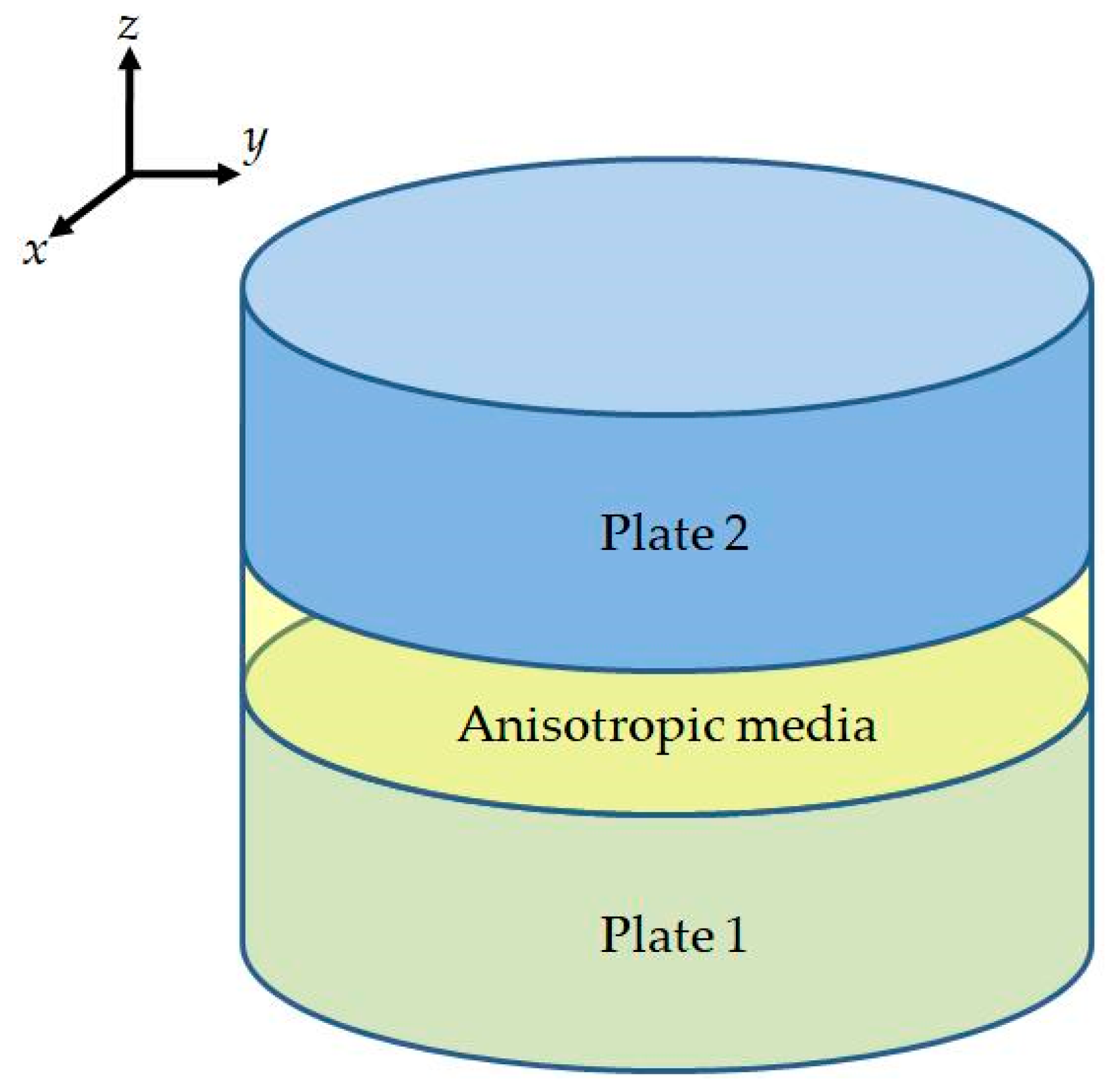
Figure 2.
The schematic of the system under investigation. The space can be considered to be divided into three regions with corresponding permittivities.
Figure 2.
The schematic of the system under investigation. The space can be considered to be divided into three regions with corresponding permittivities.

Figure 3.
Φ and Φ0 vs. δ. ε10/ε3x0 = 1.5 and ε20/ε3x0 = 0.8. Φ is shown with the solid line and Φ0 is shown with the red dash line. The positive value indicates that the force is attractive, while the negative value indicates that the force is repulsive. (a) ε10 > ε3x0 > ε20 > ε3z0; (b) ε3z0 > ε10 > ε3x0 > ε20.
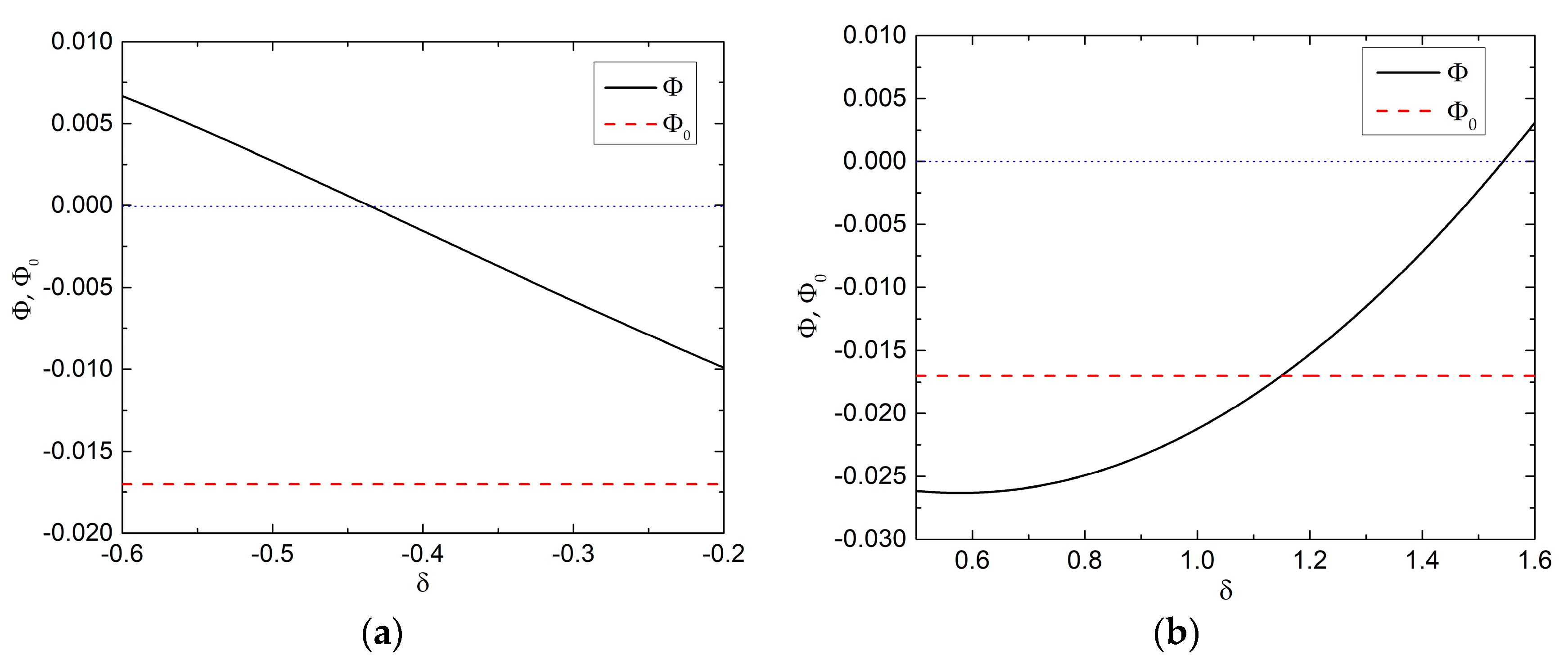
Figure 4.
Φ and Φ0 vs. δ. ε10/ε3x0 = 1.5, ε20/ε3x0 = 1.1 and ε3z0 > ε10 > ε20 > ε3x0. Φ is shown with the solid line and Φ0 is shown with the red dash line. The positive value indicates that the force is attractive, while the negative value indicates that the force is repulsive.
Figure 4.
Φ and Φ0 vs. δ. ε10/ε3x0 = 1.5, ε20/ε3x0 = 1.1 and ε3z0 > ε10 > ε20 > ε3x0. Φ is shown with the solid line and Φ0 is shown with the red dash line. The positive value indicates that the force is attractive, while the negative value indicates that the force is repulsive.

Figure 5.
The Casimir force when dispersion is considered. The positive value indicates that the force is attractive, while the negative value indicates that the force is repulsive. The horizontal dash-dot line indicates F = 0 and the intersections between this line and other curves indicate the reverses of the direction of the force. (a) The frequency dependent pemittivities (The models of dispersion relation are described in Appendix B); (b) F(a) vs. a; (c) The impact of anisotropy of intervening media; (d) F(a) vs. δ.

© 2018 by the authors. Licensee MDPI, Basel, Switzerland. This article is an open access article distributed under the terms and conditions of the Creative Commons Attribution (CC BY) license (http://creativecommons.org/licenses/by/4.0/).
Share and Cite
MDPI and ACS Style
Deng, G.; Pei, L.; Hu, N.; Liu, Y.; Zhu, J.-R. The Impact of the Anisotropy of the Media between Parallel Plates on the Casimir Force. Symmetry 2018, 10, 61. https://doi.org/10.3390/sym10030061
AMA Style
Deng G, Pei L, Hu N, Liu Y, Zhu J-R. The Impact of the Anisotropy of the Media between Parallel Plates on the Casimir Force. Symmetry. 2018; 10(3):61. https://doi.org/10.3390/sym10030061
Chicago/Turabian StyleDeng, Gang, Ling Pei, Ni Hu, Yang Liu, and Jin-Rong Zhu. 2018. "The Impact of the Anisotropy of the Media between Parallel Plates on the Casimir Force" Symmetry 10, no. 3: 61. https://doi.org/10.3390/sym10030061
Note that from the first issue of 2016, this journal uses article numbers instead of page numbers. See further details here.