The LHC Higgs Boson Discovery: Updated Implications for Finite Unified Theories and the SUSY Breaking Scale
by
Sven Heinemeyer
1,2,3, 
Myriam Mondragón
4,
Gregory Patellis
5,*,
Nicholas Tracas
5 and
George Zoupanos
5,6 1
Instituto de Física Teórica, Universidad Autónoma de Madrid Cantoblanco, 28049 Madrid, Spain
2
Campus of International Excellence UAM+CSIC, Cantoblanco, 28049 Madrid, Spain
3
Instituto de Física de Cantabria (CSIC-UC), E-39005 Santander, Spain
4
Instituto de Física, Universidad Nacional Autónoma de México, A.P. 20-364, Mexico City 01000, Mexico
5
Physics Department, National Technical University, 157 80 Zografou, Greece
6
Max-Planck Institut für Physik, Föhringer Ring 6, D-80805 München, Germany
*
Author to whom correspondence should be addressed.
Symmetry 2018, 10(3), 62; https://doi.org/10.3390/sym10030062
Submission received: 12 February 2018
/
Revised: 27 February 2018
/
Accepted: 27 February 2018
/
Published: 7 March 2018
(This article belongs to the Special Issue Symmetry in Quantum Field Theory)
Abstract
:Finite Unified Theories (FUTs) are supersymmetric Grand Unified Theories, which can be made finite to all orders in perturbation theory, based on the principle of the reduction of couplings. The latter consists of searching for renormalization group invariant relations among parameters of a renormalizable theory holding to all orders in perturbation theory. FUTs have proven very successful so far. In particular, they predicted the top quark mass one and half years before its experimental discovery, while around five years before the Higgs boson discovery, a particular FUT was predicting the light Higgs boson in the mass range ∼121–126 GeV, in striking agreement with the discovery at LHC. Here, we review the basic properties of the supersymmetric theories and in particular finite theories resulting from the application of the method of reduction of couplings in their dimensionless and dimensionful sectors. Then, we analyze the phenomenologically-favored FUT, based on SU(5). This particular FUT leads to a finiteness constrained version of the Minimal SUSY Standard Model (MSSM), which naturally predicts a relatively heavy spectrum with colored supersymmetric particles above 2.7 TeV, consistent with the non-observation of those particles at the LHC. The electroweak supersymmetric spectrum starts below 1 TeV, and large parts of the allowed spectrum of the lighter might be accessible at CLIC. The FCC-hhwill be able to fully test the predicted spectrum.
1. Introduction
In 2012, the discovery of a new particle at the LHC was announced [1,2]. Within theoretical and experimental uncertainties, the new particle is compatible with predictions for the Higgs boson of the Standard Model (SM) [3,4], constituting a milestone in the quest for understanding the physics of Electroweak Symmetry Breaking (EWSB). However, taking the experimental results and the respective uncertainties into account, also many models beyond the SM can accommodate the data. Furthermore, the hierarchy problem, the neutrino masses, the dark matter, the over twenty free parameters of the model, just to name some questions, ask for a more fundamental theory to answer some, if not all, of those.
Therefore, one of the main aims of this fundamental theory is to relate these free parameters, or rephrasing it, to achieve a reduction of these parameters in favor of a smaller number (or ideally only one). This reduction is usually based on the introduction of a larger symmetry, rendering the theory more predictive. Very good examples are the Grand Unified Theories (GUTs) [5,6,7,8,9] and their supersymmetric extensions [10,11]. The case of minimal is one example, where the number of couplings is reduced to one due to the corresponding unification. Data from LEP [12] suggested that a global Supersymmetry (SUSY) [10,11] is required in order for the prediction to be viable. Relations among the Yukawa couplings are also suggested in GUTs. For example, the predicts the ratio of the tau to the bottom mass [13] in the SM. GUTs introduce, however, new complications such as the different ways of breaking this larger symmetry, as well as new degrees of freedom.
A way to relate the Yukawa and the gauge sector, in other words achieving Gauge-Yukawa Unification (GYU) [14,15,16], seems to be a natural extension of the GUTs. The possibility that SUSY [17] plays such a role is highly limited due to the prediction of light mirror fermions. Other phenomenological drawbacks appear in composite models and superstring theories.
A complementary approach is to search for all-loop Renormalization Group Invariant (RGI) relations [18,19], which hold below the Planck scale and are preserved down to the unification scale [14,15,16,20,21,22,23,24,25]. With this approach, Gauge-Yukawa Unification (GYU) is possible. A remarkable point is that, assuming finiteness at one-loop in gauge theories, RGIrelations that guarantee finiteness to all orders in perturbation theory can be found [26,27,28].
The above approach seems to need SUSY as an essential ingredient. However, the breaking of SUSY has to be understood as well, since it provides the SM with several predictions for its free parameters. Actually, the RGI relation searches have been extended to the Soft SUSY Breaking (SSB) sector [25,29,30,31] relating parameters of mass dimension one and two. This is indeed possible to be done on the RGI surface, which is defined by the solution of the reduction equations.
Applying the reduction of couplings method to SUSY theories has led to very interesting phenomenological developments. Previously, an appealing “universal” set of soft scalar masses was assumed in the SSB sector of SUSY theories, given that, apart from economy and simplicity: (1) they are part of the constraints that preserve finiteness up to two loops [32,33]; (2) they are RGI up to two loops in more general SUSY gauge theories, subject to the condition known as [29]; and (3) they appear in the attractive dilaton-dominated SUSY breaking superstring scenarios [34,35,36]. However, further studies exhibited problems all due to the restrictive nature of the “universality” assumption for the scalar masses. For instance: (a) in Finite Unified Theories (FUTs) the universality predicts that the lightest SUSY particle is a charged particle, namely the superpartner of the lepton ; (b) the Minimal SUSY Standard Model (MSSM) with universal soft scalar masses is inconsistent with the attractive radiative electroweak symmetry breaking; and worst of all, (c) the universal soft scalar masses lead to charge and/or color breaking minima deeper than the standard vacuum [37]. Therefore, there have been attempts to relax this constraint without loosing its attractive features. First, an interesting observation was made that in GYU theories, there exists an RGI sum rule for the soft scalar masses at lower orders; at one loop for the non-finite case [38] and at two loops for the finite case [39]. The sum rule manages to overcome the above unpleasant phenomenological consequences. Moreover, it was proven [40] that the sum rule for the soft scalar masses is RGI to all orders for both the general and the finite case. Finally, the exact -function for the soft scalar masses in the Novikov–Shifman–Vainshtein–Zakharov (NSVZ) scheme [41,42,43] for the softly-broken SUSY QCDhas been obtained [40]. the use of RGI both in the dimensionful and dimensionless sector, together with the above-mentioned sum rule, allows for the construction of realistic and predictive all-loop finite SUSY GUTs, also with interesting predictions, as was shown in [14,20,22,31,44,45,46,47,48].
This paper is organized as follows. In Section 2, we review the theoretical basis of the method of the reduction of couplings, which is extended in Section 2 to the dimensionful parameters. Section 3 is devoted to finiteness in the dimensionless sector of a SUSY theory in some detail. In Section 4, we discuss the implications of the method of reduction of couplings in the SUSY breaking sector of an SUSY theory including the finite case. Then, in Section 5, we review the best Finite Unified Modelselected previously on the basis of agreement with the known experimental data at the time [45]. the current setup of experimental constraints and predictions is briefly reviewed in Section 6 and applied to our best Finite Unified Model in Section 7, including in particular the latest improvements in the prediction of the light Higgs boson mass (as implemented in FeynHiggs). Our conclusions can be found in Section 8.
2. Theoretical Basis
In this section, we outline the idea of the reduction of couplings. Any RGI relation among couplings (which does not depend on the renormalization scale explicitly) can be expressed, in the implicit form , which has to satisfy the Partial Differential Equation (PDE):
where is the -function of . This PDE is equivalent to a set of ordinary differential equations, the so-called Reduction Equations (REs) [18,19,49],
where g and are the primary coupling and its -function, and the counting on a does not include g. Since maximally () independent RGI “constraints” in the A-dimensional space of couplings can be imposed by the ’s, one could in principle express all the couplings in terms of a single coupling g. However, a closer look at the set of Equation (2) reveals that their general solutions contain as many integration constants as the number of equations themselves. Thus, using such integration constants, we have just traded an integration constant for each ordinary renormalized coupling, and consequently, these general solutions cannot be considered as reduced ones. The crucial requirement in the search for RGE relations is to demand power series solutions to the REs,
which preserve perturbative renormalizability. Such an ansatz fixes the corresponding integration constant in each of the REs and picks up a special solution out of the general one. Remarkably, the uniqueness of such power series solutions can be decided already at the one-loop level [18,19,49]. To illustrate this, let us assume that the -functions have the form:
where ⋯ stands for higher order terms and ’s are symmetric in . We then assume that the ’s with have been uniquely determined. To obtain ’s, we insert the power series (3) into the REs (2) and collect terms of and find:
where the r.h.s. is known by assumption, and:
Therefore, the ’s for all for a given set of ’s can be uniquely determined if for all .
As will be clear later by examining specific examples, the various couplings in SUSY theories have the same asymptotic behavior. Therefore, searching for a power series solution of the form (3) to the REs (2) is justified. This is not the case in non-SUSY theories, although the deeper reason for this fact is not fully understood.
The possibility of coupling unification described in this section is without any doubt attractive, because the “completely reduced” theory contains only one independent coupling, but it can be unrealistic. Therefore, one often would like to impose fewer RGI constraints, and this is the idea of partial reduction [50,51].
Reduction of Dimension One and Two Parameters
The reduction of couplings was originally formulated for massless theories on the basis of the Callan–Symanzik equation [18,19]. The extension to theories with massive parameters is not straightforward if one wants to keep the generality and the rigor on the same level as for the massless case; one has to fulfill a set of requirements coming from the renormalization group equations, the Callan–Symanzik equations, etc. along with the normalization conditions imposed on irreducible Green’s functions [52]. There has been much progress in this direction starting from [25], where it was assumed that a mass-independent renormalization scheme could be employed so that all the RGfunctions have only trivial dependencies on dimensional parameters, and then, the mass parameters were introduced similarly to couplings (i.e., as a power series in the couplings). This choice was justified later in [30,53], where the scheme independence of the reduction principle has been proven generally, i.e., it was shown that apart from dimensionless couplings, pole masses and gauge parameters, the model may also involve coupling parameters carrying a dimension and masses. Therefore, here, to simplify the analysis, we follow [25], and we also use a mass-independent renormalization scheme.
We start by considering a renormalizable theory that contains a set of dimension zero couplings, , a set of L parameters with mass-dimension one, , and a set of M parameters with mass-dimension two, . The renormalized irreducible vertex function satisfies the RG equation:
where:
where is the energy scale, while are the -functions of the various dimensionless couplings , are the various matter fields and , and are the mass, trilinear coupling and wave function anomalous dimensions, respectively (where I enumerates the matter fields). In a mass independent renormalization scheme, the ’s are given by:
where , and are power series of the g’s (which are dimensionless) in perturbation theory.
We look for a reduced theory where:
are independent parameters and the reduction of the parameters left:
is consistent with the RG Equations (7) and (8). It turns out that the following relations should be satisfied:
The above relations ensure that the irreducible vertex function of the reduced theory:
has the same renormalization group flow as the original one.
The assumptions that the reduced theory is perturbatively renormalizable means that the functions , , and , defined in (10), should be expressed as a power series in the primary coupling g:
The above expansion coefficients can be found by inserting these power series into Equations (11) and (12) and requiring the equations to be satisfied at each order of g. It should be noted that the existence of a unique power series solution is a non-trivial matter: it depends on the theory, as well as on the choice of the set of independent parameters.
It should also be noted that in the case that there are no independent mass-dimension one parameters (), the reduction of these terms takes naturally the form:
where M is a mass-dimension one parameter, which could be a gaugino mass, which corresponds to the independent (gauge) coupling. In case, on top of that, there are no independent mass-dimension two parameters (), the corresponding reduction takes the analogous form:
3. Finiteness in N = 1 Supersymmetric Gauge Theories
Let us consider a chiral, anomaly-free, globally SUSY gauge theory based on a group Gwith gauge coupling constant g. The superpotential of the theory is given by:
where and are gauge invariant tensors and the matter field transforms according to the irreducible representation of the gauge group G. The renormalization constants associated with the superpotential (15), assuming that SUSY is preserved, are:
The non-renormalization theorem [54,55,56] ensures that there are no mass and cubic-interaction-term infinities, and therefore:
As a result, the only surviving possible infinities are the wave-function renormalization constants , i.e., one infinity for each field. the one-loop -function of the gauge coupling g is given by [57]:
where is the Dynkin index of and is the quadratic Casimir invariant of the adjoint representation of the gauge group G. The -functions of , by virtue of the non-renormalization theorem, are related to the anomalous dimension matrix of the matter fields as:
At one-loop level, is [57]:
where is the quadratic Casimir invariant of the representation , and . Since dimensional coupling parameters such as masses and couplings of cubic scalar field terms do not influence the asymptotic properties of a theory that we are interested in here, it is sufficient to take into account only the dimensionless SUSY couplings such as g and . Therefore, we neglect the existence of dimensional parameters and assume furthermore that are real so that are always positive numbers.
As one can see from Equations (20) and (22), all the one-loop -functions of the theory vanish if and vanish, i.e.,
The conditions for finiteness for field theories with gauge symmetry are discussed in [58], and the analysis of the anomaly-free and no-charge renormalization requirements for these theories can be found in [59]. A very interesting result is that Conditions (23) and (24) are necessary and sufficient for finiteness at the two-loop level [57,60,61,62,63].
In the case that SUSY is broken by soft terms, the requirement of finiteness in the one-loop soft breaking terms imposes further constraints among themselves [32]. In addition, the same set of conditions that are sufficient for one-loop finiteness of the soft breaking terms renders the soft sector of the theory two-loop finite [33].
The one- and two-loop finiteness Conditions (23) and (24) restrict considerably the possible choices of the irreducible representations (irreps) for a given group G, as well as the Yukawa couplings in the superpotential (15). Note in particular that the finiteness conditions cannot be applied to the Minimal SUSY Standard Model (MSSM), since the presence of a gauge group is incompatible with the condition (23), due to . This naturally leads to the expectation that finiteness should be attained at the grand unified level only, the MSSM being just the corresponding, low-energy, effective theory.
Another important consequence of one- and two-loop finiteness is that SUSY (most probably) can only be broken due to the soft breaking terms. Indeed, due to the unacceptability of gauge singlets, F-type spontaneous symmetry breaking [64] terms are incompatible with finiteness, as well as D-type [65] spontaneous breaking, which requires the existence of a gauge group.
A natural question to ask is what happens at higher-loop orders. The answer is contained in a theorem [27,66] that states the necessary and sufficient conditions to achieve finiteness at all orders. Before we discuss the theorem, let us make some introductory remarks. The finiteness conditions impose relations between gauge and Yukawa couplings. To require such relations that render the couplings mutually dependent at a given renormalization point is trivial. What is not trivial is to guarantee that relations leading to a reduction of the couplings hold at any renormalization point. As we have seen, the necessary and also sufficient condition for this to happen is to require that such relations are solutions to the REs:
and hold at all orders. Remarkably, the existence of all-order power series solutions to (25) can be decided at the one-loop level, as already mentioned.
Let us now turn to the all-order finiteness theorem [27,66], which states the conditions under which an SUSY gauge theory can become finite to all orders in the sense of vanishing -functions, that is of physical scale invariance. It is based on (a) the structure of the supercurrent in SUSY gauge theory [67,68,69] and on (b) the non-renormalization properties of chiral anomalies [26,27,66,70,71]. Details on the proof can be found in [27,66] and further discussion in [26,28,70,71,72]. Here, following mostly [72], we present a comprehensible sketch of the proof.
Consider an SUSY gauge theory, with simple Lie group G. The content of this theory is given at the classical level by the matter supermultiplets , which contain a scalar field and a Weyl spinor , and the vector supermultiplet , which contains a gauge vector field and a gaugino Weyl spinor .
Let us first recall certain facts about the theory:
(1) A massless SUSY theory is invariant under a chiral transformation R under which the various fields transform as follows:
The corresponding axial Noether current :
is conserved classically, while in the quantum case, it is violated by the axial anomaly:
From its known topological origin in ordinary gauge theories [73,74,75], one would expect the axial vector current to satisfy the Adler–Bardeen theorem and receive corrections only at the one-loop level. Indeed, it has been shown that the same non-renormalization theorem holds also in SUSY theories [26,70,71]. Therefore:
(2) The massless theory we consider is scale invariant at the classical level, and in general, there is a scale anomaly due to radiative corrections. The scale anomaly appears in the trace of the energy momentum tensor , which is traceless classically. It has the form
(3) Massless, SUSY gauge theories are classically invariant under the SUSY extension of the conformal group: the superconformal group. Examining the superconformal algebra, it can be seen that the subset of superconformal transformations consisting of translations, SUSY transformations and axial R transformations is closed under SUSY, i.e., these transformations form a representation of SUSY. It follows that the conserved currents corresponding to these transformations make up a supermultiplet represented by an axial vector superfield called the supercurrent J,
where is the current associated with Rinvariance, is the one associated with SUSY invariance and the one associated with translational invariance (energy-momentum tensor).
The anomalies of the R current , the trace anomalies of the SUSY current and the energy-momentum tensor form also a second supermultiplet, called the supertrace anomaly:
where is given in Equation (30) and:
(4) It is very important to note that the Noether current defined in (27) is not the same as the current associated with R invariance that appears in the supercurrent J in (31), but they coincide in the tree approximation. Therefore, starting from a unique classical Noether current , the Noether current is defined as the quantum extension of , which allows for the validity of the non-renormalization theorem. On the other hand, , is defined to belong to the supercurrent J, together with the energy-momentum tensor. The two requirements cannot be fulfilled by a single current operator at the same time.
Although the Noether current , which obeys (28), and the current belonging to the supercurrent multiplet J are not the same, there is a relation [27,66] between quantities associated with them:
where r was given in Equation (29). The are the non-renormalized coefficients of the anomalies of the Noether currents associated with the chiral invariances of the superpotential and (like r) are strictly one-loop quantities. The ’s are linear combinations of the anomalous dimensions of the matter fields, and and are radiative correction quantities. The structure of Equality (34) is independent of the renormalization scheme.
One-loop finiteness, i.e., vanishing of the -functions at one loop, implies that the Yukawa couplings must be functions of the gauge coupling g. To find a similar condition to all orders, it is necessary and sufficient for the Yukawa couplings to be a formal power series in g, which is the solution of the REs (25).
Theorem 1.
Consider an SUSY Yang–Mills theory, with the simple gauge group. If the following conditions are satisfied:
- 1.
- There is no gauge anomaly.
- 2.
- The gauge β-function vanishes at one loop:
- 3.
- There exist solutions of the form:to the conditions of vanishing one-loop matter fields’ anomalous dimensions:
- 4.
- These solutions are isolated and non-degenerate when considered as solutions of vanishing one-loop Yukawa β-functions:
Then, each of the solutions (36) can be uniquely extended to a formal power series in g, and the associated super Yang–Mills models depend on the single coupling constant g with a function, which vanishes at all orders.
It is important to note a few things: The requirement of isolated and non-degenerate solutions guarantees the existence of a unique formal power series solution to the reduction equations. the vanishing of the gauge function at one loop, , is equivalent to the vanishing of the R current anomaly (28). The vanishing of the anomalous dimensions at one loop implies the vanishing of the Yukawa coupling functions at that order. It also implies the vanishing of the chiral anomaly coefficients . This last property is a necessary condition for having functions vanishing at all orders. For an alternative way to find finite theories see ref. [76].
Proof.
Insert as given by the REs into the relationship (34) between the axial anomalies coefficients and the -functions. Since these chiral anomalies vanish, we get for a homogeneous equation of the form:
The solution of this equation in the sense of a formal power series in ℏ is , order by order. Therefore, due to the REs (25), , as well.
Thus, we see that finiteness and reduction of couplings are intimately related. Since an equation like Equation (34) is lacking in non-SUSY theories, one cannot extend the validity of a similar theorem in such theories. ☐
4. The SSB Sector of Reduced N = 1 SUSY and Finite Theories
As we have seen in Section 2, the method of reducing the dimensionless couplings has been extended [25], to the Soft SUSY Breaking (SSB) dimensionful parameters of SUSY theories. In addition, it was found [38] that RGI SSB scalar masses in GYU models satisfy a universal sum rule.
Consider the superpotential given by (15) along with the Lagrangian for SSB terms:
where the are the scalar parts of the chiral superfields , are the gauginos and M their unified mass.
We assume that the reduction equations admit power series solutions of the form:
If we knew higher-loop -functions explicitly, we could follow the same procedure and find higher-loop RGI relations among SSB terms. However, the -functions of the soft scalar masses are explicitly known only up to two loops. In order to obtain higher-loop results, some relations among -functions are needed.
In the case of finite theories, we assume that the gauge group is a simple group, and the one-loop -function of the gauge coupling g vanishes. According to the finiteness theorem of [27,66] and the assumption given in (40), the theory is then finite to all orders in perturbation theory, if, among others, the one-loop anomalous dimensions vanish. The one- and two-loop finiteness for can be achieved by [33]:
where … stand for higher order terms.
Now, to obtain the two-loop sum rule for soft scalar masses, we assume that the lowest order coefficients and also satisfy the diagonality relations:
respectively. Then, we find the following soft scalar-mass sum rule [16,39,77]:
for i, j, k with , where is the two-loop correction:
which vanishes for the universal choice in accordance with the previous findings of [33] (in the above relation, is the Dynkin index of the irrep).
Making use of the spurion technique [56,78,79,80,81], it is possible to find the following all-loop relations among SSB -functions [82,83,84,85,86,87]:
where , , and:
Assuming, following [83], that the relation:
among couplings is all-loop RGI and using the all-loop gauge -function of Novikov et al. [41,42,43] given by:
the all-loop RGI sum rule [40] was found:
In addition, the exact--function for in the NSVZ scheme has been obtained [40] for the first time and is given by:
Surprisingly enough, the all-loop result (53) coincides with the superstring result for the finite case in a certain class of orbifold models [39] if .
All-Loop RGI Relations in the SSB Sector
Let us now see how the all-loop results on the SSB -functions, Equations (45)–(50) lead to all-loop RGI relations. We make two assumptions:
(a) the existence of an RGI surface on which , or equivalently that:
holds, i.e., the reduction of couplings is possible, and
(b) the existence of an RGI surface on which:
holds, as well, in all orders.
Then, one can prove [88,89] that the following relations are RGI to all loops (note that in both Assumptions (a) and (b) above, we do not rely on specific solutions of these equations):
where is an arbitrary reference mass scale to be specified shortly. the assumption that:
for an RGI surface leads to:
where Equation (55) has been used. Now, let us consider the partial differential operator in Equation (48), which assuming Equation (51), becomes:
In turn, given in Equation (45) becomes:
which by integration provides us [88,90] with the generalized, i.e., including Yukawa couplings, all-loop RGI Hisano–Shifman relation [82]:
where is the integration constant and can be associated with the unification scale in GUTs or to the gravitino mass in a supergravity framework. Therefore, Equation (65) becomes the all-loop RGE Equation (57). Note that using Equations (64) and (65) can be written as:
Similarly:
Next, from Equations (51) and (65), we obtain:
while , given in Equation (46) and using Equation (67), becomes [88]:
which shows that Equation (68) is all-loop RGI. In a similar way, Equation (59) can be shown to be all-loop RGI.
Finally, we would like to emphasize that under the same Assumptions (a) and (b), the sum rule given in Equation (53) has been proven [40] to be all-loop RGI, which (using Equation (65)) gives us a generalization of Equation (60) to be applied in considerations of non-universal soft scalar masses, which are necessary in many cases. Moreover, the sum rule holds also in the more general cases, discussed in Section 2, according to which exact relations among the squared scalar and gaugino masses can be found.
5. A Successful Finite Unified Theory
We review an all-loop FUT with as the gauge group, where the reduction of couplings has been applied to the third generation of quarks and leptons. This FUT was selected previously on the basis of agreement with the known experimental data at the time [45] and was predicting the Higgs mass to be in the range 121–126 GeV almost five years before the discovery. The particle content of the model we will study, which we denote -FUT consists of the following supermultiplets: three (), needed for each of the three generations of quarks and leptons, four () and one considered as Higgs supermultiplets. When the gauge group of the finite GUT is broken, the theory is no longer finite, and we will assume that we are left with the MSSM [15,20,21,22,23,24].
A predictive GYU model, which is finite to all orders, in addition to the requirements mentioned already, should also have the following properties:
- One-loop anomalous dimensions are diagonal, i.e., .
- Three fermion generations in the irreducible representations , which obviously should not couple to the adjoint .
- The two Higgs doublets of the MSSM should mostly be made out of a pair of Higgs quintet and anti-quintet, which couple to the third generation.
After the reduction of couplings, the symmetry is enhanced, leading to the following superpotential [39,91]:
The non-degenerate and isolated solutions to give us:
and from the sum rule, we obtain:
i.e., in this case, we have only two free parameters and M for the dimensionful sector.
As already mentioned, after the gauge symmetry breaking, we assume we have the MSSM, i.e., only two Higgs doublets. This can be achieved by introducing appropriate mass terms that allow one to perform a rotation of the Higgs sector [20,24,92,93,94], in such a way that only one pair of Higgs doublets, coupled mostly to the third family, remains light and acquires vacuum expectation values. To avoid fast proton decay the usual fine tuning to achieve doublet-triplet splitting is performed, although the mechanism is not identical to minimal , since we have an extended Higgs sector.
Thus, after the gauge symmetry of the GUT theory is broken, we are left with the MSSM, with the boundary conditions for the third family given by the finiteness conditions, while the other two families are not restricted.
6. Phenomenological Constraints
In this section, we briefly review the relevant experimental constraints that we apply in our phenomenological analysis.
6.1. Flavor Constraints
We consider four types of flavor constraints to apply to the SU(5)-FUT, where SUSY is known to have significant impact. More specifically, we consider the flavor observables , , and .We do not use the latest experimental and theoretical values here. However, this has a minor impact on the general form of our results. The uncertainties are the linear combination of the experimental error and twice the theoretical uncertainty in the MSSM. We include the MSSM uncertainty also in the ratios of exp. data and SM prediction, to apply it readily to our prediction of the ratio of our MSSM and SM calculation. In the case that no specific estimate is available, we use the SM uncertainty.
For the branching ratio , we take a value from the Heavy Flavor Averaging Group (HFAG) [95,96,97,98,99,100]:
For the branching ratio , a combination of CMS and LHCb data [101,102,103,104,105,106,107,108] is used:
At the end of the phenomenological discussion, we also comment on the Cold Dark Matter (CDM) density. It is well known that the lightest neutralino, being the Lightest SUSY Particle (LSP), is an excellent candidate for CDM [114,115]. Consequently, one can in principle demand that the lightest neutralino is indeed the LSP, and parameters leading to a different LSP could be discarded.
6.2. The Light Higgs Boson Mass
The quartic couplings in the Higgs potential are given by the SM gauge couplings. As a consequence, the lightest Higgs mass is not a free parameter, but rather predicted in terms of the other parameters of the model. Higher order corrections are crucial for a precise prediction of ; see [118,119,120] for reviews.
The discovery of a Higgs boson at ATLAS and CMS in July 2012 [1,2] can be interpreted as the discovery of the light -even Higgs boson of the MSSM Higgs spectrum [121,122,123]. The experimental average for the (SM) Higgs boson mass is taken to be: [124]
and adding in quadrature a 3 (2) GeV theory uncertainty [125,126,127] for the Higgs mass calculation in the MSSM, we arrive at an allowing range of:
We used the code FeynHiggs [125,127,128,129,130,131,132,133] (Version 2.14.0 beta) to predict the lightest Higgs boson mass. the evaluation of the Higgs masses with FeynHiggs is based on the combination of a Feynman-diagrammatic calculation and a resummation of the (sub)leading and logarithms contributions of the (general) type of in all orders of perturbation theory. This combination ensures a reliable evaluation of also for large SUSY scales. Several refinements in the combination of the fixed order log resummed calculation have been included w.r.t. previous versions; see [127]. They resulted not only in a more precise evaluation for high SUSY mass scales, but in particular in a downward shift of at the level of for large SUSY masses.
7. Numerical Analysis
In this section, we will analyze the particle spectrum predicted in the -FUT . Since the gauge symmetry is spontaneously broken below , the finiteness conditions do not restrict the renormalization properties at low energies, and all that remains are boundary conditions on the gauge and Yukawa couplings (71), the (41) relation and the soft scalar-mass sum rule at .
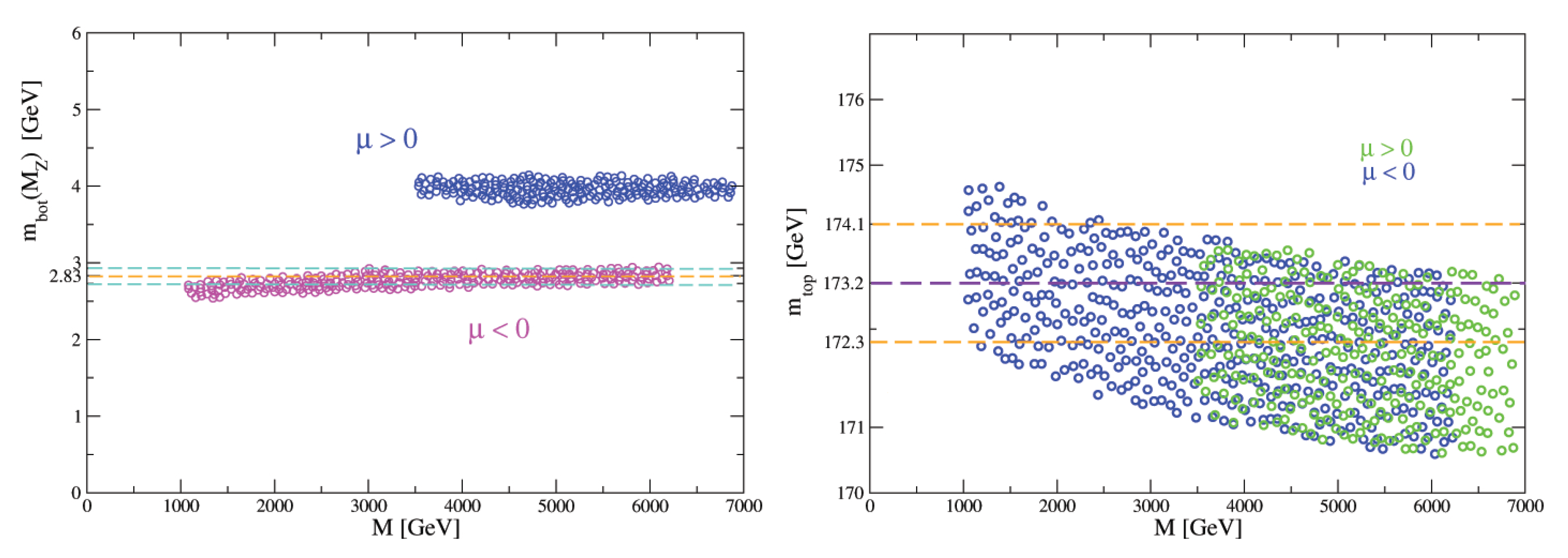
In Figure 1, we show the -FUT predictions for and as a function of the unified gaugino mass M, for the two cases and . We use the experimental value of the top quark pole mass as [111]. We did not include the latest LHC/Tevatron combination, leading to [134], which would have a negligible impact on our analysis.
The bottom mass is calculated at to avoid uncertainties that come from running down to the pole mass; the leading SUSY radiative corrections to the bottom and tau masses have been taken into account [135]. We use the following value for the bottom mass at [111],
The bounds on the and the mass clearly single out , as the solution most compatible with these experimental constraints.
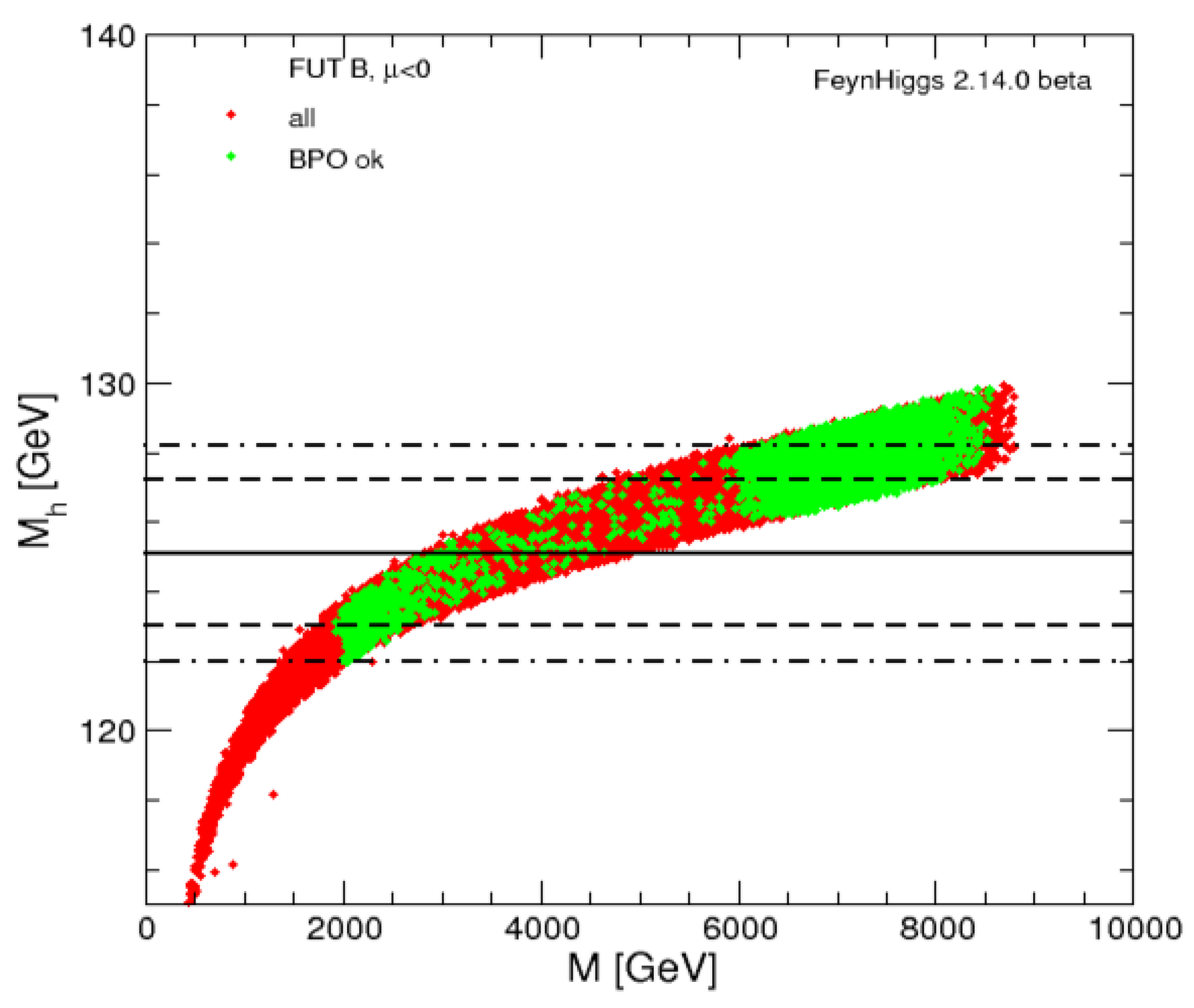
As was already mentioned, for the lightest Higgs boson mass, we used the code FeynHiggs (2.14.0 beta). the prediction for of -FUT with is shown in Figure 2, in a range where the unified gaugino mass varies from 0.5 TeV ≲M≲ 9 TeV. The green points include the B-physics constraints. One should keep in mind that these predictions are subject to a theory uncertainty of 3 (2) GeV [125]. Older analysis, including in particular less refined evaluations of the light Higgs boson mass, are given in [46,136,137].
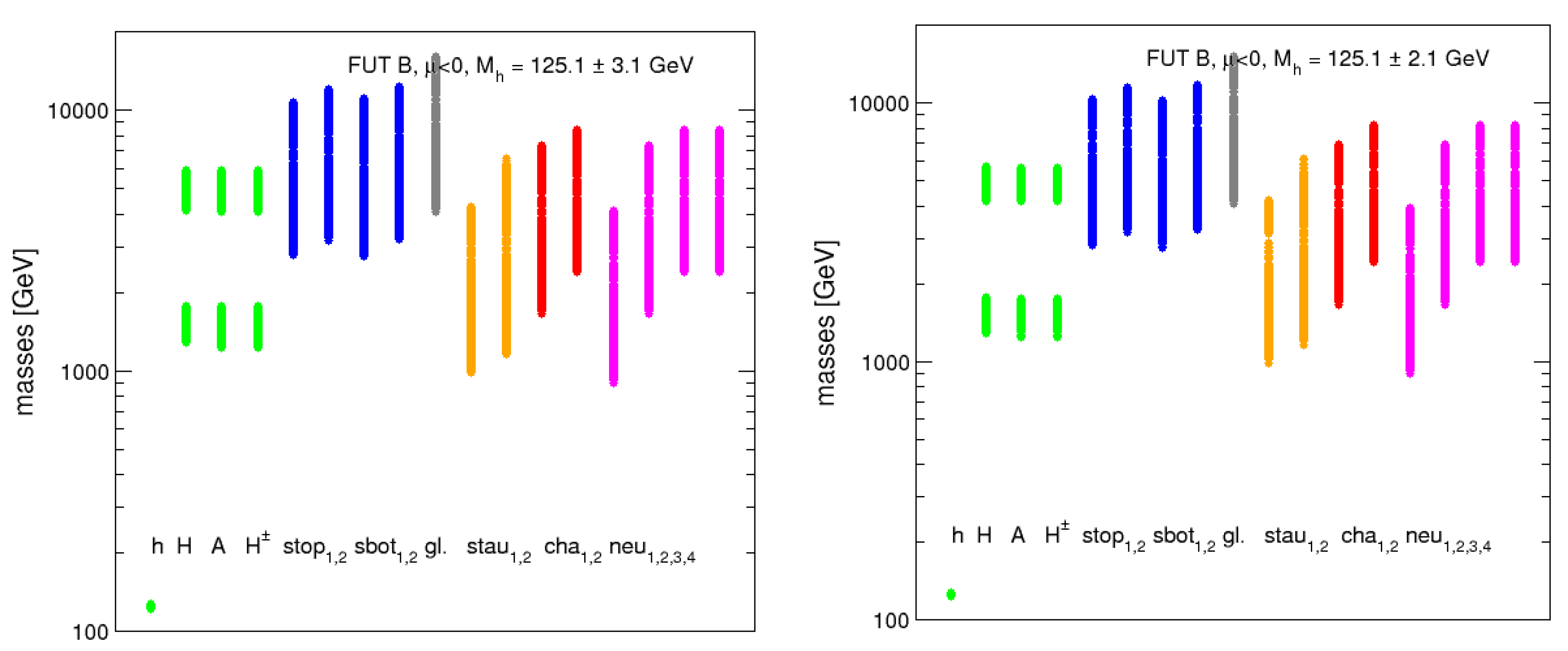
The allowed values of the Higgs mass put a limit on the allowed values of the SUSY masses, as can be seen in Figure 3. In the left (right) plot, we impose as discussed above. In particular, very heavy colored SUSY particles are favored (nearly independent of the uncertainty), in agreement with the non-observation of those particles at the LHC [138,139]. Overall, the allowed colored SUSY masses would remain unobservable at the (HL-)LHC, the ILC or CLIC. However, the colored spectrum would be accessible at the FCC-hh [140], as could the full heavy Higgs boson spectrum. On the other hand, the Lightest Observable SUSY Particle (LSOP) is the scalar tau. Some parts of the allowed spectrum of the lighter scalar tau or the lighter charginos/neutralinos might be accessible at CLIC with .
In Table 1, we show two example spectra of the -FUT (with ) which span the mass range of the parameter space that is in agreement with the B-physics observables and the Higgs-boson mass measurement. We give the lightest and the heaviest spectrum for and , respectively. The four Higgs boson masses are denoted as , , and . , , and , are the scalar top, scalar bottom, gluino and scalar tau masses, respectively. and denote the chargino and neutralino masses.
We find that no point of -FUT (with ) fulfills the strict bound of Equation (77) (for our evaluation, we have used the code MicroMegas [141,142,143]). Consequently, on a more general basis, a mechanism is needed in our model to reduce the CDM abundance in the early universe. This issue could, for instance, be related to another problem, that of neutrino masses. This type of mass cannot be generated naturally within the class of Finite Unified Theories that we are considering in this paper, although a non-zero value for neutrino masses has clearly been established [111]. However, the class of FUTs discussed here can, in principle, be easily extended by introducing bilinear R-parity violating terms that preserve finiteness and introduce the desired neutrino masses [144,145]. R-parity violation [146,147,148,149] would have a small impact on the collider phenomenology presented here (apart from the fact that SUSY search strategies could not rely on a ‘missing energy’ signature), but remove the CDM bound of Equation (77) completely. The details of such a possibility in the present framework attempting to provide the models with realistic neutrino masses will be discussed elsewhere. Other mechanisms, not involving R-parity violation (and keeping the ‘missing energy’ signature), that could be invoked if the amount of CDM appears to be too large, concern the cosmology of the early universe. For instance, “thermal inflation” [150] or “late time entropy injection” [151] could bring the CDM density into agreement with the WMAP measurements. This kind of modification of the physics scenario neither concerns the theory basis nor the collider phenomenology, but could have a strong impact on the CDM bounds (lower values than those permitted by Equation (77) are naturally allowed if a particle other than the lightest neutralino constitutes CDM).
8. Conclusions
The MSSM is considered a very attractive candidate for describing physics beyond the SM. However, the serious problem of the SM having too many free parameters is further proliferated in the MSSM. Assuming a GUT beyond the scale of gauge coupling unification, based on the idea that a Particle Physics Theoryshould be more symmetric at higher scales, seems to fit the MSSM. On the other hand, the unification scenario seems to be unable to further reduce the number of free parameters.
Attempting to reduce the free parameters of a theory, a new approach was proposed in [18,19] based on the possible existence of RGI relations among couplings. Although this approach could uncover further symmetries, its application opens new horizons, as well. At least the Finite Unified Theories seem to comprise a very promising field for applying the reduction approach. In the FUT case, the discovery of RGI relations among couplings above the unification scale ensures at the same time finiteness to all orders.
The discussion in the previous sections of this paper shows that the predictions of the particular FUT discussed here are impressive. In addition, one could add some comments on a successful FUT from the theoretical side, as well. The developments on treating the problem of divergencies include string and non-commutative theories, as well as SUSY theories [152,153], supergravity [154,155,156,157,158] and the AdS/CFT correspondence [159]. It is very interesting that the FUT discussed here includes many ideas that have survived phenomenological and theoretical tests, as well as the ultraviolet divergence problem. It is actually solving that problem in a minimal way.
We concentrated our examination on the predictions of one particular Finite Unified Theory, including the restrictions of third generation quark masses and B-physics observables. The model, -FUT (with ), is consistent with all the phenomenological constraints. Compared to our previous analyses [46,47,136,137], the improved evaluation of prefers a heavier (Higgs) spectrum and thus in general allows only a very heavy SUSY spectrum. The colored spectrum could easily escapes the (HL-)LHC searches, but can likely be tested at the FCC-hh. The lower part of the electroweak spectrum could be accessible at CLIC.
Acknowledgments
We thank H.Bahl, T. Hahn, W. Hollik, D. Lüst and E. Seiler for helpful discussions. The work of Sven Heinemeyer is supported in part by the MEINCOPSpain under Contract FPA2016-78022-P, in part by the Spanish Agencia Estatal de Investigación (AEI), the EU Fondo Europeo de Desarrollo Regional (FEDER) through the project FPA2016-78645-P, and in part by the AEI through the grant IFTCentro de Excelencia Severo Ochoa SEV-2016-0597. The work of M.M. is partly supported by UNAM PAPIITthrough Grant IN111518. The work of Nicholas Tracas and George Zoupanos is supported by the COST actions CA15108 and CA16201. George Zoupanos thanks the MPIMunich for hospitality and the A.v.Humboldt Foundation for support.
Author Contributions
Sven Heinemeyer contributed to the numerical analysis and to the phenomenology part of the paper, Myriam Mondragón and Nicholas Tracas contributed in the theory part and numerical analysis, Gregory Patellis contributed in the numerical analysis and George Zoupanos contributed to the theory part.
Conflicts of Interest
The authors declare no conflict of interest.
References
- Aad, G.; Abajyan, T.; Abbott, B.; Abdallah, J.; Khalek, S.A.; Abdelalim, A.A.; Abdinov, O.; Aben, R.; Abi, B.; Abolins, M.; et al. Observation of a new particle in the search for the Standard Model Higgs boson with the ATLAS detector at the LHC. Phys. Lett. B 2012, 716, 1–29. [Google Scholar] [CrossRef] [Green Version]
- Chatrchyan, S.; Khachatryan, V.; Sirunyan, A.M.; Tumasyan, A.; Adam, W.; Aguilo, E.; Bergauer, T.; Dragicevic, M.; Erö, J.; Fabjan, C.; et al. Observation of a new boson at a mass of 125 GeV with the CMS experiment at the LHC. Phys. Lett. B 2012, 716, 30–61. [Google Scholar] [CrossRef]
- ATLAS Collaboration; Aad, G. Combined Measurements of the Mass and Signal Strength of the Higgs-Like Boson with the ATLAS Detector Using up to 25 fb−1 of Proton-Proton Collision Data; ATLAS-CONF-2013-014; ATLAS Collaboration: Geneva, Switzerland, 2013. [Google Scholar]
- Chatrchyan, S.; Khachatryan, V.; Sirunyan, A.M.; Tumasyan, A.; Adam, W.; Bergauer, T.; Dragicevic, M.; Erö, J.; Fabjan, C.; Friedl, M.; et al. Observation of a new boson with mass near 125 GeV in pp collisions at = 7 and 8 TeV. JHEP 2013, 1306, 81. [Google Scholar] [CrossRef] [Green Version]
- Pati, J.C.; Salam, A. Is Baryon Number Conserved? Phys. Rev. Lett. 1973, 31, 661. [Google Scholar] [CrossRef]
- Georgi, H.; Glashow, S.L. Unity of All Elementary Particle Forces. Phys. Rev. Lett. 1974, 32, 438. [Google Scholar] [CrossRef]
- Georgi, H.; Quinn, H.R.; Weinberg, S. Hierarchy of Interactions in Unified Gauge Theories. Phys. Rev. Lett. 1974, 33, 451. [Google Scholar] [CrossRef]
- Carlson, C.E. Particles and Fields: Williamsburg 1974. AIP Conference Proceedings No. 23; American INstitute of Physics: New York, NY, USA, 1975; 688p. [Google Scholar]
- Fritzsch, H.; Minkowski, P. Unified Interactions of Leptons and Hadrons. Ann. Phys. 1975, 93, 193–266. [Google Scholar] [CrossRef]
- Dimopoulos, S.; Georgi, H. Softly Broken Supersymmetry and SU (5). Nucl. Phys. B 1981, 193, 150–162. [Google Scholar] [CrossRef]
- Sakai, N. Naturalness in Supersymmetric Guts. Z. Phys. C 1981, 11, 153–157. [Google Scholar] [CrossRef]
- Amaldi, U.; de Boer, W.; Furstenau, H. Comparison of grand unified theories with electroweak and strong coupling constants measured at LEP. Phys. Lett. B 1991, 260, 447–455. [Google Scholar] [CrossRef]
- Buras, A.J.; Ellis, J.R.; Gaillard, M.K.; Nanopoulos, D.V. Aspects of the Grand Unification of Strong, Weak and Electromagnetic Interactions. Nucl. Phys. B 1978, 135, 66–92. [Google Scholar] [CrossRef]
- Kubo, J.; Mondragon, M.; Olechowski, M.; Zoupanos, G. Testing gauge Yukawa unified models by M(t). Nucl. Phys. B 1996, 479, 25–45. [Google Scholar] [CrossRef]
- Kubo, J.; Mondragon, M.; Zoupanos, G. Unification beyond GUTs: Gauge Yukawa unification. Acta Phys. Polon. B 1997, 27, 3911–3944. [Google Scholar]
- Kobayashi, T.; Kubo, J.; Mondragon, M.; Zoupanos, G. Exact finite and gauge-Yukawa unified theories and their predictions. Acta Phys. Polon. B 1999, 30, 2013–2027. [Google Scholar]
- Fayet, P. Spontaneous Generation of Massive Multiplets and Central Charges in Extended Supersymmetric Theories. Nucl. Phys. B 1979, 149, 137–169. [Google Scholar] [CrossRef]
- Zimmermann, W. Reduction in the Number of Coupling Parameters. Commun. Math. Phys. 1985, 97, 211–225. [Google Scholar] [CrossRef]
- Oehme, R.; Zimmermann, W. Relation between Effective Couplings for Asymptotically Free Models. Commun. Math. Phys. 1985, 97, 569–582. [Google Scholar] [CrossRef]
- Kapetanakis, D.; Mondragon, M.; Zoupanos, G. Finite unified models. Z. Phys. C 1993, 60, 181–185. [Google Scholar] [CrossRef]
- Kubo, J.; Mondragon, M.; Zoupanos, G. Reduction of couplings and heavy top quark in the minimal SUSY GUT. Nucl. Phys. B 1994, 424, 291–307. [Google Scholar] [CrossRef]
- Kubo, J.; Mondragon, M.; Tracas, N.D.; Zoupanos, G. Gauge Yukawa unification in asymptotically nonfree theories. Phys. Lett. B 1995, 342, 155–162. [Google Scholar] [CrossRef]
- Kubo, J.; Mondragon, M.; Olechowski, M.; Zoupanos, G. Gauge Yukawa unification and the top–bottom hierarchy. arXiv, 1995; arXiv:hep-ph/9510279. [Google Scholar]
- Mondragon, M.; Zoupanos, G. Finite unified theories and the top quark mass. Nucl. Phys. Proc. Suppl. C 1995, 37, 98–105. [Google Scholar] [CrossRef]
- Kubo, J.; Mondragon, M.; Zoupanos, G. Perturbative unification of soft supersymmetry breaking terms. Phys. Lett. B 1996, 389, 523–532. [Google Scholar] [CrossRef]
- Piguet, O.; Sibold, K. Nonrenormalization Theorems of Chiral Anomalies and Finiteness in Supersymmetric Yang-Mills Theories. Int. J. Mod. Phys. A 1986, 1, 913–942. [Google Scholar] [CrossRef]
- Lucchesi, C.; Piguet, O.; Sibold, K. Vanishing Beta Functions in N = 1 Supersymmetric Gauge Theories. Helv. Phys. Acta 1988, 61, 321–344. [Google Scholar]
- Lucchesi, C.; Zoupanos, G. All order finiteness in N = 1 SYM theories: Criteria and applications. Fortsch. Phys. 1997, 45, 129–143. [Google Scholar] [CrossRef]
- Jack, I.; Jones, D.R.T. Renormalization group invariance and universal soft supersymmetry breaking. Phys. Lett. B 1995, 349, 294–299. [Google Scholar] [CrossRef]
- Zimmermann, W. Scheme independence of the reduction principle and asymptotic freedom in several couplings. Commun. Math. Phys. 2001, 219, 221–245. [Google Scholar] [CrossRef]
- Mondragón, M.; Tracas, N.D.; Zoupanos, G. Reduction of Couplings in the MSSM. Phys. Lett. B 2014, 728, 51–57. [Google Scholar] [CrossRef] [Green Version]
- Jones, D.R.T.; Mezincescu, L.; Yao, Y.P. Soft Breaking of Two Loop Finite N = 1 Supersymmetric Gauge Theories. Phys. Lett. B 1984, 148, 317–322. [Google Scholar] [CrossRef]
- Jack, I.; Jones, D.R.T. Soft supersymmetry breaking and finiteness. Phys. Lett. B 1994, 333, 372–379. [Google Scholar] [CrossRef]
- Ibanez, L.E.; Lust, D. Duality anomaly cancellation, minimal string unification and the effective low-energy Lagrangian of 4-D strings. Nucl. Phys. B 1992, 382, 305–361. [Google Scholar] [CrossRef]
- Kaplunovsky, V.S.; Louis, J. Model independent analysis of soft terms in effective supergravity and in string theory. Phys. Lett. B 1993, 306, 269–275. [Google Scholar] [CrossRef]
- Brignole, A.; Ibanez, L.E.; Munoz, C. Towards a theory of soft terms for the supersymmetric Standard Model. Nucl. Phys. B 1994, 422, 125–171. [Google Scholar] [CrossRef]
- Casas, J.A.; Lleyda, A.; Munoz, C. Problems for supersymmetry breaking by the dilaton in strings from charge and color breaking. Phys. Lett. B 1996, 380, 59–67. [Google Scholar] [CrossRef]
- Kawamura, Y.; Kobayashi, T.; Kubo, J. Soft scalar mass sum rule in gauge Yukawa unified models and its superstring interpretation. Phys. Lett. B 1997, 405, 64–70. [Google Scholar] [CrossRef]
- Kobayashi, T.; Kubo, J.; Mondragon, M.; Zoupanos, G. Constraints on finite soft supersymmetry breaking terms. Nucl. Phys. B 1998, 511, 45–68. [Google Scholar] [CrossRef]
- Kobayashi, T.; Kubo, J.; Zoupanos, G. Further all loop results in softly broken supersymmetric gauge theories. Phys. Lett. B 1998, 427, 291–299. [Google Scholar] [CrossRef]
- Novikov, V.A.; Shifman, M.A.; Vainshtein, A.I.; Zakharov, V.I. Instanton Effects in Supersymmetric Theories. Nucl. Phys. B 1983, 229, 407–420. [Google Scholar] [CrossRef]
- Novikov, V.A.; Shifman, M.A.; Vainshtein, A.I.; Zakharov, V.I. Beta Function in Supersymmetric Gauge Theories: Instantons Versus Traditional Approach. Phys. Lett. B 1986, 166, 329–333. [Google Scholar] [CrossRef]
- Shifman, M.A. Little miracles of supersymmetric evolution of gauge couplings. Int. J. Mod. Phys. A 1996, 11, 5761–5784. [Google Scholar] [CrossRef]
- Kubo, J.; Mondragon, M.; Shoda, S.; Zoupanos, G. Gauge Yukawa unification in SO(10) SUSY GUTs. Nucl. Phys. B 1996, 469, 3–20. [Google Scholar] [CrossRef]
- Heinemeyer, S.; Mondragon, M.; Zoupanos, G. Confronting Finite Unified Theories with Low-Energy Phenomenology. JHEP 2008, 807, 135. [Google Scholar] [CrossRef]
- Heinemeyer, S.; Mondragon, M.; Zoupanos, G. Finite Theories after the discovery of a Higgs-like boson at the LHC. Phys. Lett. B 2013, 718, 1430–1435. [Google Scholar] [CrossRef]
- Heinemeyer, S.; Mondragon, M.; Zoupanos, G. Finite Theories Before and After the Discovery of a Higgs Boson at the LHC. Fortsch. Phys. 2013, 61, 969–993. [Google Scholar] [CrossRef]
- Heinemeyer, S.; Mondragon, M.; Zoupanos, G. The LHC Higgs boson discovery: Implications for Finite Unified Theories. Int. J. Mod. Phys. A 2014, 29, 1430032. [Google Scholar] [CrossRef]
- Oehme, R. Reduction and Reparametrization of Quantum Field Theories. Prog. Theor. Phys. Suppl. 1986, 86, 215–237. [Google Scholar] [CrossRef]
- Kubo, J.; Sibold, K.; Zimmermann, W. Higgs and Top Mass from Reduction of Couplings. Nucl. Phys. B 1985, 259, 331–350. [Google Scholar] [CrossRef]
- Kubo, J.; Sibold, K.; Zimmermann, W. New Results in the Reduction of the Standard Model. Phys. Lett. B 1989, 220, 185–190. [Google Scholar] [CrossRef]
- Piguet, O.; Sibold, K. Reduction of Couplings in the Presence of Parameters. Phys. Lett. B 1989, 229, 83–88. [Google Scholar] [CrossRef]
- Breitenlohner, P.; Maison, D. Gauge and mass parameter dependence of renormalized Green’s functions. Commun. Math. Phys. 2001, 219, 179–190. [Google Scholar] [CrossRef]
- Wess, J.; Zumino, B. A Lagrangian Model Invariant under Supergauge Transformations. Phys. Lett. B 1974, 49, 52–54. [Google Scholar] [CrossRef]
- Iliopoulos, J.; Zumino, B. Broken Supergauge Symmetry and Renormalization. Nucl. Phys. B 1974, 76, 310–332. [Google Scholar] [CrossRef]
- Fujikawa, K.; Lang, W. Perturbation Calculations for the Scalar Multiplet in a Superfield Formulation. Nucl. Phys. B 1975, 88, 61–76. [Google Scholar] [CrossRef]
- Parkes, A.; West, P.C. Finiteness in Rigid Supersymmetric Theories. Phys. Lett. B 1984, 138, 99–104. [Google Scholar] [CrossRef]
- Rajpoot, S.; Taylor, J.G. On Finite Quantum Field Theories. Phys. Lett. B 1984, 147, 91–95. [Google Scholar] [CrossRef]
- Rajpoot, S.; Taylor, J.G. Towards Finite Quantum Field Theories. Int. J. Theor. Phys. 1986, 25, 117–138. [Google Scholar] [CrossRef]
- West, P.C. The Yukawa beta Function in N = 1 Rigid Supersymmetric Theories. Phys. Lett. B 1984, 137, 371–373. [Google Scholar] [CrossRef]
- Jones, D.R.T.; Mezincescu, L. The Chiral Anomaly and a Class of Two Loop Finite Supersymmetric Gauge Theories. Phys. Lett. B 1984, 138, 293–295. [Google Scholar] [CrossRef]
- Jones, D.R.T.; Parkes, A.J. Search for a Three Loop Finite Chiral Theory. Phys. Lett. B 1985, 160, 267–270. [Google Scholar] [CrossRef]
- Parkes, A.J. Three Loop Finiteness Conditions in N = 1 Superyang-mills. Phys. Lett. B 1985, 156, 73–79. [Google Scholar] [CrossRef]
- O’Raifeartaigh, L. Spontaneous Symmetry Breaking for Chiral Scalar Superfields. Nucl. Phys. B 1975, 96, 331–352. [Google Scholar] [CrossRef]
- Fayet, P.; Iliopoulos, J. Spontaneously Broken Supergauge Symmetries and Goldstone Spinors. Phys. Lett. B 1974, 51, 461–464. [Google Scholar] [CrossRef]
- Lucchesi, C.; Piguet, O.; Sibold, K. Necessary and Sufficient Conditions for All Order Vanishing Beta Functions in Supersymmetric Yang-Mills Theories. Phys. Lett. B 1988, 201, 241–244. [Google Scholar] [CrossRef]
- Ferrara, S.; Zumino, B. Transformation Properties of the Supercurrent. Nucl. Phys. B 1975, 87, 207–220. [Google Scholar] [CrossRef]
- Piguet, O.; Sibold, K. The Supercurrent in N = 1 Supersymmetrical Yang-Mills Theories. 1. The Classical Case. Nucl. Phys. B 1982, 196, 428–446. [Google Scholar] [CrossRef]
- Piguet, O.; Sibold, K. The Supercurrent in N = 1 Supersymmetrical Yang-Mills Theories. 2. Renormalization. Nucl. Phys. B 1982, 196, 447–460. [Google Scholar] [CrossRef]
- Piguet, O.; Sibold, K. Nonrenormalization Theorems of Chiral Anomalies and Finiteness. Phys. Lett. B 1986, 177, 373–376. [Google Scholar] [CrossRef]
- Ensign, P.; Mahanthappa, K.T. The Supercurrent and the Adler-bardeen Theorem in Coupled Supersymmetric Yang-Mills Theories. Phys. Rev. D 1987, 36, 3148. [Google Scholar] [CrossRef]
- Piguet, O. Supersymmetry, ultraviolet finiteness and grand unification. arXiv, 1996; arXiv:hep-th/9606045. [Google Scholar]
- Alvarez-Gaume, L.; Ginsparg, P.H. The Topological Meaning of Nonabelian Anomalies. Nucl. Phys. B 1984, 243, 449–474. [Google Scholar] [CrossRef]
- Bardeen, W.A.; Zumino, B. Consistent and Covariant Anomalies in Gauge and Gravitational Theories. Nucl. Phys. B 1984, 244, 421–453. [Google Scholar] [CrossRef]
- Zumino, B.; Wu, Y.S.; Zee, A. Chiral Anomalies, Higher Dimensions, and Differential Geometry. Nucl. Phys. B 1984, 239, 477–507. [Google Scholar] [CrossRef]
- Leigh, R.G.; Strassler, M.J. Exactly marginal operators and duality in four-dimensional N = 1 supersymmetric gauge theory. Nucl. Phys. B 1995, 447, 95–133. [Google Scholar] [CrossRef]
- Mondragon, M.; Zoupanos, G. Higgs mass prediction in finite unified theories. Acta Phys. Polon. B 2003, 34, 5459–5468. [Google Scholar] [CrossRef]
- Delbourgo, R. Superfield Perturbation Theory and Renormalization. Nuovo Cim. A 1975, 25, 646–656. [Google Scholar] [CrossRef]
- Salam, A.; Strathdee, J.A. Feynman Rules for Superfields. Nucl. Phys. B 1975, 86, 142–152. [Google Scholar] [CrossRef]
- Grisaru, M.T.; Siegel, W.; Rocek, M. Improved Methods for Supergraphs. Nucl. Phys. B 1979, 159, 429–450. [Google Scholar] [CrossRef]
- Girardello, L.; Grisaru, M.T. Soft Breaking of Supersymmetry. Nucl. Phys. B 1982, 194, 65–76. [Google Scholar] [CrossRef]
- Hisano, J.; Shifman, M.A. Exact results for soft supersymmetry breaking parameters in supersymmetric gauge theories. Phys. Rev. D 1997, 56, 5475. [Google Scholar] [CrossRef]
- Jack, I.; Jones, D.R.T. The Gaugino Beta function. Phys. Lett. B 1997, 415, 383. [Google Scholar] [CrossRef]
- Avdeev, L.V.; Kazakov, D.I.; Kondrashuk, I.N. Renormalizations in softly broken SUSY gauge theories. Nucl. Phys. B 1998, 510, 289–312. [Google Scholar] [CrossRef]
- Kazakov, D.I. Exploring softly broken SUSY theories via Grassmannian Taylor expansion. Phys. Lett. B 1999, 449, 201–206. [Google Scholar] [CrossRef]
- Kazakov, D.I. Finiteness of soft terms in finite N = 1 SUSY gauge theories. Phys. Lett. B 1998, 421, 211–216. [Google Scholar] [CrossRef]
- Jack, I.; Jones, D.R.T.; Pickering, A. Renormalization invariance and the soft Beta functions. Phys. Lett. B 1998, 426, 73–77. [Google Scholar] [CrossRef]
- Jack, I.; Jones, D.R.T. RG invariant solutions for the soft supersymmetry breaking parameters. Phys. Lett. B 1999, 465, 148–154. [Google Scholar] [CrossRef]
- Kobayashi, T.; Kubo, J.; Mondragon, M.; Zoupanos, G. Finite and gauge-Yukawa unified theories: Theory and predictions. AIP Conf. Proc. 1999, 490, 279–309. [Google Scholar] [CrossRef]
- Karch, A.; Kobayashi, T.; Kubo, J.; Zoupanos, G. Infrared behavior of softly broken SQCD and its dual. Phys. Lett. B 1998, 441, 235–342. [Google Scholar] [CrossRef]
- Mondragon, M.; Zoupanos, G. Finite unified theories. J. Phys. Conf. Ser. 2009, 171, 012095. [Google Scholar] [CrossRef]
- Hamidi, S.; Schwarz, J.H. A Realistic Finite Unified Theory? Phys. Lett. B 1984, 147, 301–306. [Google Scholar] [CrossRef]
- Jones, D.R.T.; Raby, S. A Two Loop Finite Supersymmetric SU(5) Theory: Towards a Theory of Fermion Masses. Phys. Lett. B 1984, 143, 137–141. [Google Scholar] [CrossRef]
- Leon, J.; Perez-Mercader, J.; Quiros, M.; Ramirez-Mittelbrunn, J. A Sensible Finite Su(5) Susy Gut? Phys. Lett. B 1985, 156, 66–72. [Google Scholar] [CrossRef]
- Misiak, M.; Asatrian, H.M.; Bieri, K.; Czakon, M.; Czarnecki, A.; Ewerth, T.; Ferroglia, A.; Gambino, P.; Gorbahn, M.; Greub, C.; et al. Estimate of at . Phys. Rev. Lett. 2007, 98, 22002. [Google Scholar] [CrossRef] [PubMed]
- Ciuchini, M.; Degrassi, G.; Gambino, P.; Giudice, G.F. Next-to-leading QCD corrections to B → X(s) gamma in supersymmetry. Nucl. Phys. B 1998, 534, 3–20. [Google Scholar] [CrossRef]
- Degrassi, G.; Gambino, P.; Giudice, G.F. B → X(s gamma) in supersymmetry: Large contributions beyond the leading order. JHEP 2000, 12, 9. [Google Scholar] [CrossRef]
- Carena, M.; Garcia, D.; Nierste, U.; Wagner, C.E.M. b → sγ and supersymmetry with large tan β. Phys. Lett. B 2001, 499, 141–146. [Google Scholar] [CrossRef]
- D’Ambrosio, G.; Giudice, G.F.; Isidori, G.; Strumia, A. Minimal flavor violation: An Effective field theory approach. Nucl. Phys. B 2002, 645, 155–187. [Google Scholar] [CrossRef]
- Asner, D.; Banerjee, S.; Bernhard, R.; Blyth, S.; Bozek, A.; Bozzi, C.; Cassel, D.G.; Cavoto, G.; Cibinetto, G.; Coleman, J.; et al. Averages of b-hadron, c-hadron, and τ-lepton properties. arXiv, 2010; arXiv:1010.1589. [Google Scholar]
- Buras, A.J. Relations between Δ M(s, d) and B(s, d) → μ in models with minimal flavor violation. Phys. Lett. B 2003, 566, 115–119. [Google Scholar] [CrossRef]
- Isidori, G.; Straub, D.M. Minimal Flavour Violation and Beyond. Eur. Phys. J. C 2012, 72, 2103. [Google Scholar] [CrossRef]
- Bobeth, C.; Gorbahn, M.; Hermann, T.; Misiak, M.; Stamou, E.; Steinhauser, M. Bs,d → l+l− in the Standard Model with Reduced Theoretical Uncertainty. Phys. Rev. Lett. 2014, 112, 101801. [Google Scholar] [CrossRef] [PubMed]
- Hermann, T.; Misiak, M.; Steinhauser, M. Three-loop QCD corrections to Bs → μ+μ−. JHEP 2013, 1312, 97. [Google Scholar] [CrossRef]
- Bobeth, C.; Gorbahn, M.; Stamou, E. Electroweak Corrections to Bs,d → ℓ+ℓ−. Phys. Rev. D 2014, 89, 34023. [Google Scholar] [CrossRef]
- Aaij, R.; Adeva, B.; Adinolfi, M.; Adrover, C.; Affolder, A.; Ajaltouni, Z.; Albrecht, J.; Alessio, F.; Alexander, M.; Ali, S.; et al. Measurement of the → μ+μ− branching fraction and search for B0 → μ+μ− decays at the LHCb experiment. Phys. Rev. Lett. 2013, 111, 101805. [Google Scholar] [CrossRef] [PubMed]
- Quertenmont, L.; Beluffi, C.; Bruno, G.L.; Castello, R.; Caudron, A.; Ceard, L.; Da Silveira, G.G.; Delaere, C.; Du Pree, T.; Favart, D.; et al. Measurement of the B(s) to mu+ mu- branching fraction and search for B0 to mu+ mu- with the CMS Experiment. Phys. Rev. Lett. 2013, 111, 101804. [Google Scholar] [CrossRef]
- CMS and LHCb Collaborations. Combination of Results on the Rare Decays B0(s) → μ+μ− from the CMS and LHCb Experiments; Technical Report; CMS-PAS-BPH-13-007; CERN-LHCb-CONF-2013-012; CERN: Geneva, Switzerland, 2013. [Google Scholar]
- Isidori, G.; Paradisi, P. Hints of large tan(beta) in flavour physics. Phys. Lett. B 2006, 639, 499–507. [Google Scholar] [CrossRef]
- Isidori, G.; Mescia, F.; Paradisi, P.; Temes, D. Flavour physics at large tan(beta) with a Bino-like LSP. Phys. Rev. D 2007, 75, 115019. [Google Scholar] [CrossRef]
- Olive, K.A.; Particle Data Group. Review of Particle Physics. Chin. Phys. C 2014, 38, 90001. [Google Scholar] [CrossRef]
- Buras, A.J.; Gambino, P.; Gorbahn, M.; Jager, S.; Silvestrini, L. epsilon-prime/epsilon and rare K and B decays in the MSSM. Nucl. Phys. B 2001, 592, 55–91. [Google Scholar] [CrossRef]
- LHCb Collaboration. Precision measurement of the oscillation frequency with the decay → . New J. Phys. 2013, 15, 53021. [Google Scholar] [CrossRef]
- Goldberg, H. Constraint on the Photino Mass from Cosmology. Phys. Rev. Lett. 1983, 50, 1419. [Google Scholar] [CrossRef]
- Ellis, J.R.; Hagelin, J.S.; Nanopoulos, D.V.; Olive, K.A.; Srednicki, M. Supersymmetric Relics from the Big Bang. Nucl. Phys. B 1984, 238, 453–476. [Google Scholar] [CrossRef]
- Larson, D.; Dunkley, J.; Hinshaw, G.; Komatsu, E.; Nolta, M.R.; Bennett, C.L.; Gold, B.; Halpern, M.; Hill, R.S.; Jarosik, N.; et al. Seven-Year Wilkinson Microwave Anisotropy Probe (WMAP) Observations: Cosmological Interpretation. Astrophys. J. Suppl. 2011, 192, 18. [Google Scholar] [CrossRef]
- Komatsu, E.; Bennett, C.L.; Barnes, C.; Bean, R.; Bennett, C.L.; Doré, O.; Dunkley, J.; Gold, B.; Greason, M.R.; Halpern, M.; et al. Results from the Wilkinson Microwave Anisotropy Probe. PTEP 2014, 2014, 06B102. [Google Scholar] [CrossRef]
- Heinemeyer, S. MSSM Higgs physics at higher orders. Int. J. Mod. Phys. A 2006, 21, 2659–2772. [Google Scholar] [CrossRef]
- Heinemeyer, S.; Hollik, W.; Weiglein, G. Electroweak precision observables in the minimal supersymmetric standard model. Phys. Rep. 2006, 425, 265–368. [Google Scholar] [CrossRef]
- Djouadi, A. The Anatomy of electro-weak symmetry breaking. II. The Higgs bosons in the minimal supersymmetric model. Phys. Rep. 2008, 459, 1–241. [Google Scholar] [CrossRef]
- Heinemeyer, S.; Stal, O.; Weiglein, G. Interpreting the LHC Higgs Search Results in the MSSM. Phys. Lett. B 2012, 710, 201–206. [Google Scholar] [CrossRef] [Green Version]
- Bechtle, P.; Heinemeyer, S.; Stal, O.; Stefaniak, T.; Weiglein, G.; Zeune, L. MSSM Interpretations of the LHC Discovery: Light or Heavy Higgs? Eur. Phys. J. 2013, 73, 2354. [Google Scholar] [CrossRef]
- Bechtle, P.; Haber, H.E.; Heinemeyer, S.; Stål, O.; Stefaniak, T.; Weiglein, G.; Zeune, L. The Light and Heavy Higgs Interpretation of the MSSM. Eur. Phys. J. C 2017, 77, 67. [Google Scholar] [CrossRef]
- ATLAS and CMS Collaborations. Combined Measurement of the Higgs Boson Mass in pp Collisions at =7 and 8 TeV with the ATLAS and CMS Experiments. Phys. Rev. Lett. 2015, 114, 191803. [Google Scholar] [CrossRef]
- Degrassi, G.; Heinemeyer, S.; Hollik, W.; Slavich, P.; Weiglein, G. Towards high precision predictions for the MSSM Higgs sector. Eur. Phys. J. C 2003, 28, 133–143. [Google Scholar] [CrossRef]
- Buchmueller, O.; Dolan, M.J.; Ellis, J.; Hahn, T.; Heinemeyer, S.; Hollik, W.; Marrouche, J.; Olive, K.A.; Rzehak, H.; de Vries, K.J.; et al. Implications of Improved Higgs Mass Calculations for Supersymmetric Models. Eur. Phys. J. C 2014, 74, 2809. [Google Scholar] [CrossRef] [PubMed]
- Bahl, H.; Heinemeyer, S.; Hollik, W.; Weiglein, G. Reconciling EFT and hybrid calculations of the light MSSM Higgs-boson mass. Eur. Phys. J. C 2018, 78, 57. [Google Scholar] [CrossRef]
- Heinemeyer, S.; Hollik, W.; Weiglein, G. FeynHiggs: A Program for the calculation of the masses of the neutral CP even Higgs bosons in the MSSM. Comput. Phys. Commun. 2000, 124, 76–89. [Google Scholar] [CrossRef]
- Heinemeyer, S.; Hollik, W.; Weiglein, G. The Masses of the neutral CP—Even Higgs bosons in the MSSM: Accurate analysis at the two loop level. Eur. Phys. J. C 1999, 9, 343–366. [Google Scholar] [CrossRef] [Green Version]
- Frank, M.; Hahn, T.; Heinemeyer, S.; Hollik, W.; Rzehak, H.; Weiglein, G. The Higgs Boson Masses and Mixings of the Complex MSSM in the Feynman-Diagrammatic Approach. JHEP 2007, 702, 47. [Google Scholar] [CrossRef]
- Hahn, T.; Heinemeyer, S.; Hollik, W.; Rzehak, H.; Weiglein, G. FeynHiggs: A program for the calculation of MSSM Higgs-boson observables—Version 2.6.5. Comput. Phys. Commun. 2009, 180, 1426–1427. [Google Scholar] [CrossRef]
- Hahn, T.; Heinemeyer, S.; Hollik, W.; Rzehak, H.; Weiglein, G. High-Precision Predictions for the Light CP-Even Higgs Boson Mass of the Minimal Supersymmetric Standard Model. Phys. Rev. Lett. 2014, 112, 141801. [Google Scholar] [CrossRef] [PubMed]
- Bahl, H.; Hollik, W. Precise prediction for the light MSSM Higgs boson mass combining effective field theory and fixed-order calculations. Eur. Phys. J. C 2016, 76, 499. [Google Scholar] [CrossRef]
- ATLAS and CDF and CMS and D0 Collaborations. First combination of Tevatron and LHC measurements of the top-quark mass. arXiv, 2014; arXiv:1403.4427. [Google Scholar]
- Carena, M.; Garcia, D.; Nierste, U.; Wagner, C.E.M. Effective Lagrangian for the interaction in the MSSM and charged Higgs phenomenology. Nucl. Phys. B 2000, 577, 88. [Google Scholar] [CrossRef]
- Heinemeyer, S.; Mondragon, M.; Zoupanos, G. Futs and the Higgs-boson. Int. J. Mod. Phys. Conf. Ser. 2012, 13, 118. [Google Scholar] [CrossRef]
- Heinemeyer, S.; Mondragon, M.; Zoupanos, G. Finite unified theories and their predicitions. Phys. Part. Nucl. 2013, 44, 299–315. [Google Scholar] [CrossRef]
- Supersymmetry Searches. Available online: https://twiki.cern.ch/twiki/bin/view/AtlasPublic/SupersymmetryPublicResults (accessed on 11 February 2017).
- CMS Supersymmetry Physics Results. Available online: https://twiki.cern.ch/twiki/bin/view/CMSPublic/PhysicsResultsSUS (accessed on 11 February 2017).
- Mangano, M. Physics at the FCC-hh, a 100 TeV pp Collider; CERN Yellow Report CERN 2017-003-M; CERN: Genève, Switzerland, 2017. [Google Scholar]
- Belanger, G.; Boudjema, F.; Pukhov, A.; Semenov, A. MicrOMEGAs: A Program for calculating the relic density in the MSSM. Comput. Phys. Commun. 2002, 149, 103–120. [Google Scholar] [CrossRef]
- Belanger, G.; Boudjema, F.; Pukhov, A.; Semenov, A. micrOMEGAs: Version 1.3. Comput. Phys. Commun. 2006, 174, 577–604. [Google Scholar] [CrossRef]
- Barducci, D.; Belanger, G.; Bernon, J.; Boudjema, F.; da Silva, J.; Kraml, S.; Laa, U.; Pukhov, A. Collider limits on new physics within micrOMEGAs_4.3. Comput. Phys. Commun. 2018, 222, 327–338. [Google Scholar] [CrossRef]
- Valle, J.W.F. Neutrino mass: Theory, data and interpretation. PoS Corfu 1998, arXiv:hep-ph/990722298. [Google Scholar]
- Diaz, M.A.; Hirsch, M.; Porod, W.; Romao, J.C.; Valle, J.W.F. Solar neutrino masses and mixing from bilinear R parity broken supersymmetry: Analytical versus numerical results. Phys. Rev. D 2003, 68, 13009. [Google Scholar] [CrossRef]
- Dreiner, H.K. An Introduction to explicit R-parity violation. Adv. Ser. Direct. High Energy Phys. 2010, 21, 565–583. [Google Scholar] [CrossRef]
- Bhattacharyya, G. A Brief Review of R-Parity Violating Couplings; Presented at the ‘Beyond the Desert’; Castle Ringberg: Tegernsee, Germany, 1997. [Google Scholar]
- Allanach, B.C.; Dedes, A.; Dreiner, H.K. Bounds on R-parity violating couplings at the weak scale and at the GUT scale. Phys. Rev. D 1999, 60, 75014. [Google Scholar] [CrossRef] [Green Version]
- Romao, J.C.; Valle, J.W.F. Neutrino masses in supersymmetry with spontaneously broken R parity. Nucl. Phys. B 1992, 381, 87–108. [Google Scholar] [CrossRef]
- Lyth, D.H.; Stewart, E.D. Thermal inflation and the moduli problem. Phys. Rev. D 1996, 53, 1784. [Google Scholar] [CrossRef]
- Gelmini, G.B.; Gondolo, P. Neutralino with the right cold dark matter abundance in (almost) any supersymmetric model. Phys. Rev. D 2006, 74, 23510. [Google Scholar] [CrossRef]
- Mandelstam, S. Light Cone Superspace and the Ultraviolet Finiteness of the N = 4 Model. Nucl. Phys. B 1983, 213, 149–168. [Google Scholar] [CrossRef]
- Brink, L.; Lindgren, O.; Nilsson, B.E.W. The Ultraviolet Finiteness of the N = 4 Yang-Mills Theory. Phys. Lett. B 1983, 123, 323–328. [Google Scholar] [CrossRef]
- Bern, Z.; Carrasco, J.J.; Dixon, L.J.; Johansson, H.; Roiban, R. The Ultraviolet Behavior of N = 8 Supergravity at Four Loops. Phys. Rev. Lett. 2009, 103, 81301. [Google Scholar] [CrossRef] [PubMed]
- Kallosh, R. On UV Finiteness of the Four Loop N = 8 Supergravity. JHEP 2009, 909, 116. [Google Scholar] [CrossRef]
- Bern, Z.; Carrasco, J.J.; Dixon, L.J.; Johansson, H.; Kosower, D.A.; Roiban, R. Three-Loop Superfiniteness of N = 8 Supergravity. Phys. Rev. Lett. 2007, 98, 161303. [Google Scholar] [CrossRef] [PubMed]
- Bern, Z.; Dixon, L.J.; Roiban, R. Is N = 8 supergravity ultraviolet finite? Phys. Lett. B 2007, 644, 265–271. [Google Scholar] [CrossRef]
- Green, M.B.; Russo, J.G.; Vanhove, P. Ultraviolet properties of maximal supergravity. Phys. Rev. Lett. 2007, 98, 131602. [Google Scholar] [CrossRef] [PubMed]
- Maldacena, J.M. The Large N limit of superconformal field theories and supergravity. Int. J. Theor. Phys. 1999, 38, 1113–1133. [Google Scholar] [CrossRef] [Green Version]
Figure 1.
The bottom quark mass at the Z boson scale (left) and top quark pole mass (right) are shown as a function of M for both signs of .
Figure 1.
The bottom quark mass at the Z boson scale (left) and top quark pole mass (right) are shown as a function of M for both signs of .

Figure 2.
The lightest Higgs mass, , as a function of M for the Finite Unified Theory (FUT) model with . The green points are the ones that satisfy the B-physics constraints.
Figure 2.
The lightest Higgs mass, , as a function of M for the Finite Unified Theory (FUT) model with . The green points are the ones that satisfy the B-physics constraints.

Figure 3.
The (left,right) plots show the spectrum of the -FUT (with ) model after imposing the constraint . The light (green) points are the various Higgs boson masses; the dark (blue) points following are the two scalar top and bottom masses; the gray ones are the gluino masses; then come the scalar tau masses in orange (light gray); the darker (red) points to the right are the two chargino masses; followed by the lighter shaded (pink) points indicating the neutralino masses.


Table 1.
Two example spectra of the -FUT (with ) . All masses are in GeV and rounded to 1 (0.1) GeV (for the light Higgs mass).
Table 1.
Two example spectra of the -FUT (with ) . All masses are in GeV and rounded to 1 (0.1) GeV (for the light Higgs mass).
| lightest | 123.1 | 1533 | 1528 | 1527 | 2800 | 3161 | 2745 | 3219 | 4077 |
| heaviest | 127.2 | 4765 | 4737 | 4726 | 10,328 | 11,569 | 10,243 | 11,808 | 15,268 |
| lightest | 983 | 1163 | 1650 | 2414 | 900 | 1650 | 2410 | 2414 | 45 |
| heaviest | 4070 | 5141 | 6927 | 8237 | 3920 | 6927 | 8235 | 8237 | 46 |
| lightest | 122.8 | 1497 | 1491 | 1490 | 2795 | 3153 | 2747 | 3211 | 4070 |
| heaviest | 127.9 | 4147 | 4113 | 4103 | 10,734 | 12,049 | 11,077 | 12,296 | 16,046 |
| lightest | 1001 | 1172 | 1647 | 2399 | 899 | 647 | 2395 | 2399 | 44 |
| heaviest | 4039 | 6085 | 7300 | 8409 | 4136 | 7300 | 8406 | 8409 | 45 |
© 2018 by the authors. Licensee MDPI, Basel, Switzerland. This article is an open access article distributed under the terms and conditions of the Creative Commons Attribution (CC BY) license (http://creativecommons.org/licenses/by/4.0/).
Share and Cite
MDPI and ACS Style
Heinemeyer, S.; Mondragón, M.; Patellis, G.; Tracas, N.; Zoupanos, G. The LHC Higgs Boson Discovery: Updated Implications for Finite Unified Theories and the SUSY Breaking Scale. Symmetry 2018, 10, 62. https://doi.org/10.3390/sym10030062
AMA Style
Heinemeyer S, Mondragón M, Patellis G, Tracas N, Zoupanos G. The LHC Higgs Boson Discovery: Updated Implications for Finite Unified Theories and the SUSY Breaking Scale. Symmetry. 2018; 10(3):62. https://doi.org/10.3390/sym10030062
Chicago/Turabian StyleHeinemeyer, Sven, Myriam Mondragón, Gregory Patellis, Nicholas Tracas, and George Zoupanos. 2018. "The LHC Higgs Boson Discovery: Updated Implications for Finite Unified Theories and the SUSY Breaking Scale" Symmetry 10, no. 3: 62. https://doi.org/10.3390/sym10030062
Note that from the first issue of 2016, this journal uses article numbers instead of page numbers. See further details here.