Dispersion Forces Between Fields Confined to Half Spaces


1
Institut für Theoretische Physik, Universität Leipzig, Postfach 100 920, D-04009 Leipzig, Germany
2
Bogoliubov Laboratory of Theoretical Physics JINR, 141980 Dubna, Russia, and Dubna State University, 141982 Dubna, Russia
*
Author to whom correspondence should be addressed.
†
The authors contributed equally to this work.
Symmetry 2018, 10(3), 74; https://doi.org/10.3390/sym10030074
Submission received: 9 February 2018
/
Revised: 14 March 2018
/
Accepted: 15 March 2018
/
Published: 19 March 2018
(This article belongs to the Special Issue Casimir Physics and Applications)
Abstract
:We consider the Casimir effect for a scalar field interacting with another scalar field that is confined to two half spaces. This model is aimed to mimic the interaction of the photon field with matter in two slabs. We use Dirichlet boundary conditions on the interfaces for the fields in the half spaces and calculate their one-loop contribution to the wave equation for the other field. We perform the ultraviolet renormalization and develop a convenient formalism for the calculation of the vacuum energy in this configuration.
1. Introduction
In its initial formulation, the Casimir effect is the attraction between conducting plates due to the vacuum fluctuations of the electromagnetic field [1]. It was later generalized to the dispersion force between dielectric half spaces [2]. The evolution went on to include temperature of the plates and dissipation (see, e.g., [3]). The material of the plates was modeled by dipoles and/or polarization fields. An equivalent, perhaps more general, approach is macroscopic quantum electrodynamics [4,5,6]. It is a common feature of these approaches that the resulting Hamiltonian is quadratic in the fields. First papers going beyond this were on the Casimir effect with respect to graphene [7,8,9]. Here, the coupling is the usual electrodynamic one, , which is a vertex with three lines, and the corresponding Hamiltonian is no longer quadratic. However, since the spinor field describing the electrons in graphene is confined to a two-dimensional surface in three-dimensional space, the reflection coefficients could be expressed explicitly in terms of the polarization tensor of the electrons calculated within otherwise unconstrained (2 + 1)-dimensional field theory of the spinor field representing the electrons. Now, if we assume two half spaces wherein a spinor or another field is confined, we have a (3 + 1)-dimensional field theory restricted to two half spaces. We think that there is an upcoming interest in such type of calculations, which comes from the high precision measurement of dispersion forces (up to femto Newton) and that there is a challenge to account for internal dynamical properties of the interacting bodies in more detail. This means that, in future, one will be tempted to calculate Casimir forces between fields inside the bodies, electron-hole, and phonon fields, for instance.
In the present paper, we consider the simplest model of the mentioned type consisting of a scalar field in the whole space, mimicking the photon, and a field confined to the half spaces and , where L is the width of the gap between them, mimicking matter. For the interaction of the fields, we take for simplicity
where is a coupling constant with a dimension of inverse length. We assume boundary conditions on at and at in order to have a mathematically consistent model. Later, in applications, one would choose appropriate boundary conditions. The interaction part of the action is
Our notations are taken from the relativistic quantum field theory, so is the 4-coordinate, and is the coordinate parallel to the surfaces. The same notations will also be taken for the momentum variables.
The problem to be worked out is to get formulas that allow for effective numerical computation of the Casimir force or the free energy. An obstacle to surmount is the UV-divergence appearing in the loop as well as the broken translational invariance in the z-direction.
2. Scalar Field Confined to Half Spaces and the Casimir Effect
2.1. The Model
Given a scalar field confined to the half spaces and , which fulfill Dirichlet boundary conditions on and . Assume interaction with another scalar field , defined in the whole space. In one-loop approximation, the propagator of the field is given by , where is the wave operator and is the polarization operator induced by the interaction with the field in half spaces.
In the lowest order perturbation theory, the equation of motion for the field is
with the polarization operator
![Symmetry 10 00074 i001]() given by the one loop scalar field diagram. The solid line corresponds to the field and the dashed line to the field .
given by the one loop scalar field diagram. The solid line corresponds to the field and the dashed line to the field .

Using the translation invariance in all directions except the z-direction, we rewrite Equation (3) as
with
and
where we used
and .
In Equation (4), is the propagator of the field obeying Dirichlet boundary conditions. The Fourier transform in the translational invariant directions is as follows:
where the same notation as in Equation (8) is used, which is
Then, a single line of the field is
and
is the usual propagator of the scalar field .
2.2. Transition to Formula
Understanding in Equation (3) as a potential, , we use the so called formula where T and G stand for T-matrix and Green’s functon, accordingly. Employing Equations (3.112) and (10.40) in [3], we obtain the vacuum energy of the field in the presence of the half spaces:
where
with
being the free space Green’s function, i.e., the propagator of the field . In Equation (13), it is assumed that the Fourier transform in the -directions is taken, and we use Equation (7) for , and
which results in Equation (15).
In Equation (14), we took as convention arguments in the left half space and in the right half space. Integrations and are assumed. The and correspond to the potentials and in Equation (10.40) in [3]. Specifically, is from the field in (left half space). Therefore, we set for or . The other one, , is from the field in the right half space, with and , and we set for or . Further, we use the notation , as given by Equation (9), which goes without index to represent and , entering Equation (14):
The polarization tensor is defined for the interface being located in . Thus, we need in Equation (9) the propagator with Dirichlet boundary conditions at . Therefore, in place of Equations (10) and (11), we have
denotes the propagator with boundary conditions on , and denotes the propagator with boundary conditions at . The relation between them is given by Equation (18).
With these remarks, , Equation (17), can be rewritten as (accounting for the trace in Equation (13))
Doing the substitutions, , thus gives
This way, we can define
and and hold. As a result, Equation (13) turns into
and . Comparing Equation (24) with the Lifshitz formula at zero temperature, one can define the reflection coefficient of the half spaces in terms of the factors :
where we indicated the variables and parameters that depend on.
3. Polarization Operator in Half Space
In the preceding section, we have defined Equation (23) for the factors , entering the vacuum energy (Equation (24)), and introduced by Equation (4). The propagator of the field obeys Dirichlet boundary conditions at and is given by Equations (11) and (12). Inserting it into Equation (4), we obtain
where and take values . With Equation (9) and the integral representation of the -function,
we can integrate with respect to and arrive at
where .
To proceed, we divide into the translational invariant part, , arising from in the sum of Equation (27), and the remaining part, :
This will be treated separately.
We start from the translational non-invariant part, . Here, we perform the Wick rotation, and use the -representation (parametric representation) with parameters and for the factors in the denominator of Equation (27). After that, the momentum integration can be carried out and we arrive at
where the prime over the sum sign means that the term with is excluded, and
After the change of variables, and , one integration can be performed here, and we obtain
where
We insert this expression into Equation (23) and obtain the translational non-invariant part of the factor ,
In order to simplify the integration over z and , we first turn the -plane, , and then substitute . After that, the integration with respect to yields
where is given in Equation (33), and
Finally, we have
with and corresponding respectively to the terms with and with and in the sum of Equation (35):
The remaining integrals can be easily evaluated numerically. The asymptotics of are
The translational invariant part , defined in Equation (28), can be obtained from Equation (4) by dropping the index ‘’ in the propagator, which is equivalent to considering the term with in Equation (26). We denoted this term by . It has full 4-dimensional symmetry and is a function of :
The 4-dimensional Fourier transform of has the known parametric representation
where the Wick rotation is performed. In Equation (43), we introduced as the parameter of the dimensional regularization. Further, we perform the renormalization in a way where holds. This ensures that the mass of the field does not change. Technically, we achieve this by
where is an auxiliary parameter. Next we need , defined in Equation (7). Using
we obtain
Inserting Equation (46) into Equation (23), we arrive at
where the integration over z and is easily carried out:
The new, proper time representation with the parameter is then used. After integration over , we finally obtain
where . Further we’ll omit the parameter in the formulas, bearing in mind that the subtraction of Equation (44) is performed under the sign of the integration. In order to do the subtraction, we divide the integration area in Equation (49) into sectors , following, e.g., [10], p. 134. Owing to the symmetry in Equation (49), we have to account for three distinct sectors [10]:
Then, we change the variables,
and obtain
Now the translational invariant part comprises the contributions from six sectors, and half of them are equivalent. Thus, allowing for the multiplicity of the sectors, one can write
where corresponds to the contribution from the i-th sector defined in Equation (50). Integrating with respect to , we arrive at
The UV divergence is sitting in the first sector at . It is logarithmic as expected, and we have to do the subtraction of Equation (44), which does not cause any problems in our case. The integrals can be evaluated numerically. The asymptotic expansion of reads
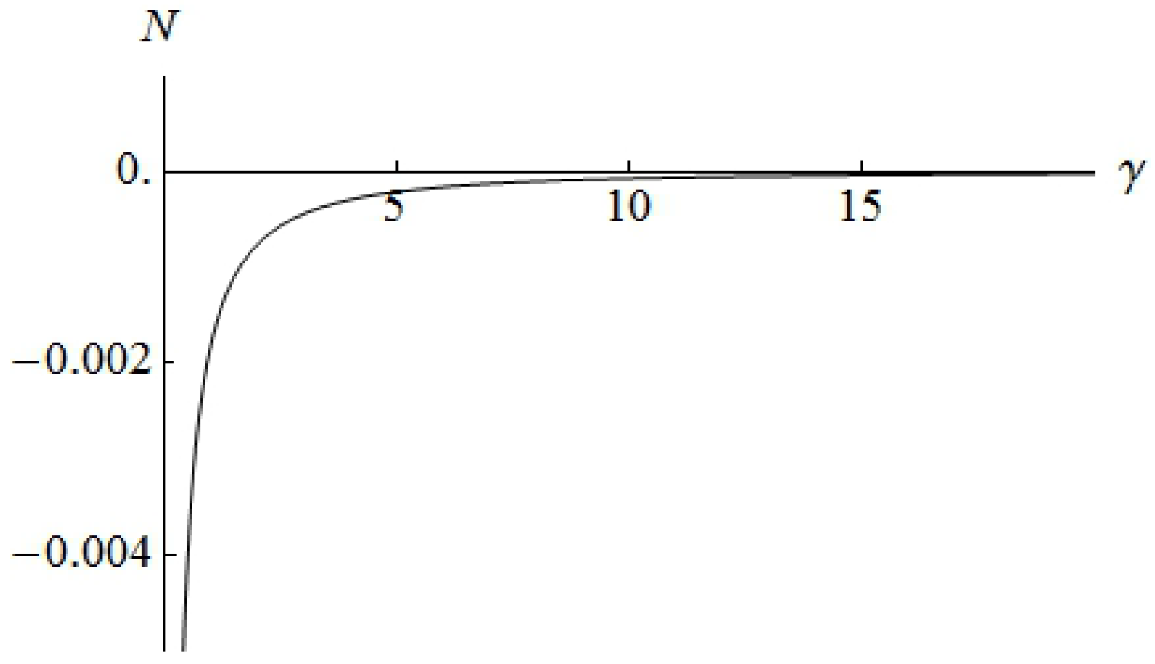
Taking the parts of Equation (23) corresponding to Equation (28), namely Equations (40), (41), (57), and (58), together, we obtain for the factor, entering Equation (24),
The factor as a function of momenta is shown in Figure 1.
4. Vacuum Energy
In the present model, the vacuum energy is defined by Equation (24) and can be rewritten in the form
For , because of (see Equations (40) and (57)), the argument of the logarithm becomes negative and the vacuum energy acquires an imaginary part, which signifies some instability within the considered model. It is known that an imaginary part of the effective action signals particle creation. Specifically, in the Casimir–Polder interaction of polarizable dipoles, such instability signals the breakdown of the dipole approximation (see, for example, [11], Equation (26) and subsequent discussion, and [12], the section after Equation (142) concerning atom–wall interaction. As the integration in Equation (61) goes from zero to infinity, the formula yields a complex vacuum energy of the field for any finite width of the gap between the half spaces.
In fact, our model is aimed to mimic the interaction of the photon field with the electron and phonon fields in a solid.As is known, the Coulomb interaction between the electrons and the phonons is screened, and the electron charge density interacts with the gradient of the phonon displacement field. This mechanism is described in many solid state textbooks (see, for instance, [13]). A characteristic feature of the model is the gradient in the interaction vertex, which turns into a momentum after Fourier transform. To account for this gradient in some way, we make the coupling momentum dependent:
such that
It is clear that this approximation is very crude, but we do not intend to describe the real electron–phonon interaction, but rather the possibility to perform calculations with such a model. As stated in the introduction, we consider the most simple model to develop the methods, which may be helpful to account for the contribution of the electron–phonon interaction to the Casimir force.
It should be mentioned that the factors play the role of reflection coefficients within the present approach for the field. Now, without the substitution according to Equation (62), these factor’s asymptotics are given by Equations (54) and (55), and, with Equation (62), they behave as Equation (63).
For the model after the substitution of Equation (62), we consider the Casimir (vacuum) energy. Its behavior for large separation can be obtained by scaling in Equation (61). We obtain the factor in front and in the logarithm, which, for , is then given by Equation (63). After the substitution of Equation (62), we obtain
5. Conclusions
In the foregoing sections, we considered the Casimir effect between two slabs in the framework of quantum field theory. A scalar field mimics the electromagnetic field, and another scalar field , which is confined by Dirichlet boundary conditions, mimics the matter inside the slabs. Both fields interact by a Yukawa coupling. For the calculation of the vacuum interaction energy, we used the TGTG formula and calculated the reflection coefficient for the field from the one-loop polarization operator of the field . The polarization operator divides into a translational non-invariant part, , and an invariant part, . While can be calculated in a straightforward manner, has an ultraviolet divergence, which can be removed by standard methods of coupling renormalization. Together, the polarization operator, and with it the reflection coefficient, can be calculated numerically (see Figure 1), and their asymptotics for large and small momenta can be obtained (Equations (58) and (60)). Finally, the Casimir energy can be calculated (see Figure 2).
As discussed in Section 4, the considered model has an instability that can be avoided by a more realistic model with a momentum dependent coupling. Thus, the main result of the paper is to demonstrate how the Casimir energy can be calculated for a (3 + 1)-dimensional matter field in the slabs within the framework of quantum field theory beyond cases with graphene where the matter field is (2 + 1)-dimensional. Thus, the path to Casimir energy calculations for more realistic models of matter is opened.
Acknowledgments
The authors acknowledge support from the Heisenberg–Landau program at JINR, Dubna.
Author Contributions
Both authors equally contributed to the research reported in this paper, and to its writing.
Conflicts of Interest
The authors declare no conflict of interest.
References
- Casimir, H.B.G.; Polder, D. The Influence of Retardation on the London-van der Waals Forces. Phys. Rev. 1948, 73, 360. [Google Scholar] [CrossRef]
- Lifshitz, E.M. The Theory of Molecular Attractive Forces Between Solids. J. Exp. Theor. Phys. 1956, 2, 73–83. [Google Scholar]
- Bordag, M.; Klimchitskaya, G.L.; Mohideen, U.; Mostepanenko, V.M. Advances in the Casimir Effect; Oxford University Press: Oxford, UK, 2009. [Google Scholar]
- Scheel, S.; Buhmann, S.Y. Macroscopic Quantum Electrodynamics—Concepts and Applications. Acta Phys. Slovaca 2008, 58, 675. [Google Scholar] [CrossRef]
- Philbin, T.G. Canonical quantization of macroscopic electromagnetism. New J. Phys. 2010, 12. [Google Scholar] [CrossRef]
- Horsley, S.A.R.; Philbin, T.G. Canonical quantization of electromagnetism in spatially dispersive media. New J. Phys. 2014, 16, 013030. [Google Scholar] [CrossRef]
- Bordag, M.; Fialkovsky, I.V.; Gitman, D.M.; Vassilevich, D.V. Casimir interaction between a perfect conductor and graphene described by the Dirac model. Phys. Rev. B 2009, 80, 245406. [Google Scholar] [CrossRef]
- Pyatkovskiy, P.K. Dynamical polarization, screening, and plasmons in gapped graphene. J. Phys. Condens. Matter 2009, 21, 025506. [Google Scholar] [CrossRef] [PubMed]
- Fialkovsky, I.V.; Vassilevich, D.V. Quantum field theory in graphene. Int. J. Mod. Phys. A 2012, 27, 1260007. [Google Scholar] [CrossRef]
- Zavialov, O. Renormalized Quantum Field Theory; Kluwer Academic Publishers: Dordrecht, The Netherlands, 1990. [Google Scholar]
- Berman, P.R.; Ford, G.W.; Milonni, P.W. Nonperturbative Calculation of the London-van der Waals Interaction Potential. Phys. Rev. A 2014, 89, 022127. [Google Scholar] [CrossRef]
- Bordag, M. Casimir and Casimir–Polder forces with dissipation from first principles. Phys. Rev. A 2017, 96, 062504. [Google Scholar] [CrossRef]
- Martin, P.; Rothen, F. Many-Body Problems and Quantum Field Theory: An Introduction; Springer: Berlin/Heidelberg, Germany, 2004. [Google Scholar]
Figure 1.
The factor playing the role of the reflection coefficient of the half space as a function of momenta , .
Figure 1.
The factor playing the role of the reflection coefficient of the half space as a function of momenta , .

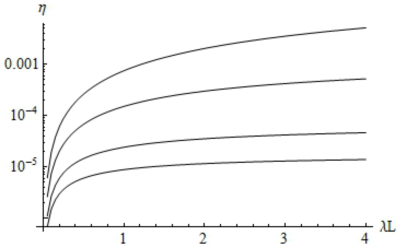
Figure 2.
The ratio, , of the Casimir energy of Equation (61) and the Casimir energy of the massless scalar field with Dirichlet boundary conditions on the plates. is drawn in logarithmic scale as a function of dimensionless separation for different vales of . From top to bottom, .
Figure 2.
The ratio, , of the Casimir energy of Equation (61) and the Casimir energy of the massless scalar field with Dirichlet boundary conditions on the plates. is drawn in logarithmic scale as a function of dimensionless separation for different vales of . From top to bottom, .

© 2018 by the authors. Licensee MDPI, Basel, Switzerland. This article is an open access article distributed under the terms and conditions of the Creative Commons Attribution (CC BY) license (http://creativecommons.org/licenses/by/4.0/).
Share and Cite
MDPI and ACS Style
Bordag, M.; Pirozhenko, I.G. Dispersion Forces Between Fields Confined to Half Spaces. Symmetry 2018, 10, 74. https://doi.org/10.3390/sym10030074
AMA Style
Bordag M, Pirozhenko IG. Dispersion Forces Between Fields Confined to Half Spaces. Symmetry. 2018; 10(3):74. https://doi.org/10.3390/sym10030074
Chicago/Turabian StyleBordag, M., and I.G. Pirozhenko. 2018. "Dispersion Forces Between Fields Confined to Half Spaces" Symmetry 10, no. 3: 74. https://doi.org/10.3390/sym10030074
Note that from the first issue of 2016, this journal uses article numbers instead of page numbers. See further details here.