Recomputing Causality Assignments on Lumped Process Models When Adding New Simplification Assumptions


Department of Computer Science and Numerical Analysis, University of Cordoba, Campus de Rabanales, 14071 Cordoba, Spain
*
Author to whom correspondence should be addressed.
Symmetry 2018, 10(4), 102; https://doi.org/10.3390/sym10040102
Submission received: 16 March 2018
/
Revised: 3 April 2018
/
Accepted: 5 April 2018
/
Published: 9 April 2018
Abstract
:This paper presents a new algorithm for the resolution of over-constrained lumped process systems, where partial differential equations of a continuous time and space model of the system are reduced into ordinary differential equations with a finite number of parameters and where the model equations outnumber the unknown model variables. Our proposal is aimed at the study and improvement of the algorithm proposed by Hangos-Szerkenyi-Tuza. This new algorithm improves the computational cost and solves some of the internal problems of the aforementioned algorithm in its original formulation. The proposed algorithm is based on parameter relaxation that can be modified easily. It retains the necessary information of the lumped process system to reduce the time cost after introducing changes during the system formulation. It also allows adjustment of the system formulations that change its differential index between simulations.
1. Introduction
There are well known reasons for modeling and simulating in engineering: testing and optimizing the design of a system before its construction, avoiding design errors, enhancing quality, reducing costs, evaluating performances, predicting responses, and so on [1]. Over the past 30 years, several modeling tools and environments have been developed [2], such as Modelica [3], Ascend [4], EcosimPro [5] and so on. Most of them are concerned with the model equations describing the system dynamics, which can be directly introduced by the user or automatically generated by the tool from some previous process description or schematic. Many physical systems are often modeled by lumped process models, particularly in the chemical process domain, where partial differential equations of a continuous time and space model are reduced into a finite set of differential-algebraic equations (DAEs) [6]. The general form of a DAE system has the following expression:
where the first equation is the differential part of the system and the second one is the algebraic part [7]. The x variables are fitted to a vector of states of , where x′ are their time-derivatives and t, the time, is the independent variable. The algebraic variables y, which are not derived, belong to . Thus, the functions f and g must be defined in some regions such as f:Ωf ⊆ → and g:Ωg ⊆ → . The set of equations in (1) must have n + m unknowns, x and y, with n + m equations in order to achieve a system with zero degrees of freedom for solvability. Modeling tools sort the equations and identify the sequence for how variables will be solved during simulation. The incidence matrix denotes which variables appear in which equation. For each variable, the matching solution determines the corresponding equation that solves this variable, that is, the causality. The Block Lower Triangular (BLT) transformation is the classical approach for this step [8] together with Tarjan’s algorithm [9]. For semi-explicit index-1 DAE models, such as (2), causalization transforms equations into assignments. In the case of high-index DAE systems, index reduction, usually by the Pantelides’ algorithm [10], must be performed to achieve an index-1 DAE or an explicit ODE model prior to matching [11]. However, dynamic simulation frequently results in numerical difficulties in the DAE resolution that can arise as a consequence of the differential index and stiffness of the DAE [12,13]. At the modeling level, an index problem can sometimes be avoided by using an alternative model formulation [14]. Therefore, the analysis of the solvability properties is basic for dynamic simulations.
In the modeling process, the DAE system is usually parameterized by the modeler with some values that are assumed to be known during the simulation. These are the design or input variables which influence the system behavior. The selection of the design variables depends highly on the problem or application area and it may greatly influence the mathematical properties of the model equation such as the differential index. Structural analysis methods can use the visual interface of modeling tools to analyze equation-variable patterns to choose the appropriate variables that have zero degrees of freedom or re-sort the DAEs to improve resolution methods [15,16]. In [17], the effect of modeling decisions on structural solvability are studied, and it was found that a change in the system specification can transform an index-1 model into a high-index system. Structural analysis methods traditionally use matrix representation and linear algebraic tools. More recent developments used a graph and combinatorial approach where the problem is addressed as a maximum weight assignment problem [18,19,20].
In the lumped process, modeling assumptions can be translated into additional mathematical relationships or constraints between model variables, equations or parameters. Adding a new modeling assumption to the system involves an additional equation, and consequently, the set of equations changes and becomes over-constrained. To recover the property of zero degrees of freedom and solve the system, two options can be chosen: removing any equation from the initial systems [21] or relaxing design variables or system parameters. As discussed later, the first option may not be a good alternative due to the logic contradictions of the initial system formulation. The second one converts the selected design variable into a new algebraic unknown to obtain a new system with zero degrees of freedom. The user must decide which design parameters are relaxed and thus, depending on this selection, different solutions can be obtained. This second method does not remove any equation from the original system, only the specification equation corresponding to the relaxed design parameter. In addition, assumption transformations may change the variable structure of the model and induce changes in the causality assignments, which need to be recomputed. Therefore, it is also important to develop algorithms that minimize the computational cost of introducing these assumptions in the initial phases of the modeling tools.
No study has been developed focused on examining the overall effect of modeling assumptions in all modeling processes. In [13], a formal representation of these assumptions is proposed to deduce basic properties of the resultant equations. The simplification assumptions, applied during the modeling phase, may seriously affect the differential index of lumped process models. In [21], adding new model assumptions and their corresponding effects on the differential index of a DAE system are studied by graph transformation. Two algorithms are proposed to follow the changes in the variable-equation assignments and the differential index. However, as will be shown later, Hangos’ method may result in contradictions and inconsistent modeling in some cases and therefore, it needs to be improved. In addition, its computational cost can be reduced.
This work proposes such improvement of Hangos’ method using the option of relaxing system parameters in the over-constrained system after adding new modeling assumptions. A polynomial time incremental algorithm is developed based on graph theory to analyze the change of differential index in the model simplification phase of the modeling process and reduce the time cost of these assumptions. The proposal can be implemented using either the Bellman-Ford or Dijkstra algorithms together with a representation of the information by minimum heaps or linked list [22,23]. According to that, the best algorithm has an almost linear time complexity if the number of assumption equations added to the system is small. The paper is structured as follows: a brief background on graph theory is given in Section 2. Section 3 describes Hangos’ method and demonstrates its limitations by means of an example. The basis of the new proposed method is introduced in Section 4 using the same illustrative example. Then, the proposed algorithm is developed and discussed. Conclusions are summarized in Section 5.
2. Bipartite Graph Preliminzaries
Next, the minimal background on bipartite graphs used to perform the proposed algorithm is discussed. A bipartite graph, denoted as B(L, R, E), is an undirected graph where the vertex set is decomposed into two disjointed sets, L and R, such that every edge e ∈ E has a vertex in L and R. In this work, DAE systems are represented as bipartite graphs where the first set consists of equation vertices and the second one consists of variable vertices. A matching in a bipartite graph is a set M ⊆ E, such that for every vertex v there is an edge e ∈ M incident to v at most; no edge in a matching can share a node. The cardinality of matching M is the number of edges covered by M. A maximum matching is a matching of maximum cardinality. A perfect matching M is a matching in which for every vertex v there is only one edge of M incident to v. Using graph theory, the equation-variable assignment problem in a DAE system can be done executing a maximum matching algorithm. If the maximum matching association includes all variables and equations (a perfect matching), the system is structurally nonsingular.
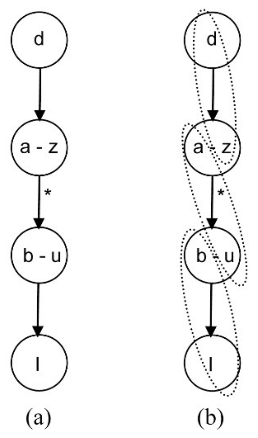
Given the equation system in (3), the corresponding bipartite graph is shown in Figure 1a where the edges which are part of a perfect matching are in bold. The form of the equations fi in (3) is irrelevant. For structural analysis, only the equation-variable relationship is considered. This optimal assignment is not unique. From this initial matching, an alternative representation, the directed graph, can be derived. In a directed graph C(U, F) induced by the bipartite graph B(L, R, E), the set of nodes is {u1, …, un} and (ui, uj) is a directed edge if and only if i ≠ j and (li, rj) ∈ E [24]. The directed graph obtained from the bipartite graph of Figure 1b is also shown on the right.
An alternating path in a bipartite graph B(L, R, E), with a matching M, is a path that interchanges the edges of M and Mc. A vertex v is free in M if there is no edge of M incident to v. An augmented path in M is an alternating path that starts and ends in a free vertex. The symmetric difference of two sets, A and B, is defined as A ∆ B = (A − B) ∪ (B − A). The cardinality of a set A is denoted as |A|. A weight function in a graph G(V,E) is a function . The weight of C ⊆ E is defined as . If p is a path in a bipartite graph with weight function w, the cost of the path p is defined as . If M is a matching and p is an augmented path into M, then, w(M ∆ p) = w(M) − α(p).
The problems of finding maximum matching and perfect matching if one exists are two of the most fundamental algorithmic graph problems. Several time polynomial algorithms have been developed. The first developments run in time O(n5/2) [25,26,27]. More recent proposals reduce the time complexity [24,28,29]. Most of them are based on a search for augmenting paths, such as the depth first search (DFS), the breadth first search (BFS) or a combination of both strategies. There also another approaches which employ a push-relabel strategy designed for maximum flow problems [30].
The proposed method is based on a search for augmenting paths. The following Theorems 1–3 establish the importance of the augmented graph in bipartite graphs [23,27,31], and allow the definition of the following Algorithm 1 to compute the matching of maximum weight onto a bipartite graph B(L, R, E) with weight function w [32].
Theorem 1.
If M is a matching and p is an augmented path into M, then M ∆ p is a matching of cardinality |M| + 1.
Theorem 2.
M is a maximum matching if and only if M does not have an augmented path.
Theorem 3.
If B(L, R, E) is a bipartite graph with weight function w, M is a matching of maximum weight for all matchings of cardinality |M| and p is an augmented path of minimum cost, then, M ∆ p is a matching of maximum weight among all the matchings of cardinality |M| + 1. Moreover, w(M ∆ p) = w(M) − α(p).
| Algorithm 1. Computing matching of maximum weight on a bipartite graph. |
| Input: A bipartite graph B(L, R, E) and weight function w. Output: Matching of maximum weight. 1: Construction of a direct graph GM(V, EM) with function weight z. 1.1: V = L ∪ R 1.2: EM is defined by: If the undirected edge (l, r) ∈ Mc then the directed edge (l, r) ∈ EM. else if the undirected edge (l, r) ∈ M then the directed edge (r, l) ∈ EM. end if That is, the set of edges EM is: EM = {(l, r)/(l, r) ∈ Mc} ∪ {(r, l)/(l, r) ∈ M} 1.3: The weight function z is defined: If (l, r) ∈ EM then z(l, r) = w (l, r). else if (r, l) ∈ EM then z(r, l) = − w((l, r) end if 1.4: Append a new vertex s linked to all free vertexes of L. 1.5: Append a new vertex t which is the destination of all free vertexes of R. 2: M := ∅ 3: while there exists an augmented path p of minimum cost into GM do 3.1: M := M ∆ p 3.2: Apply steps 1.2 and 1.3 to GM. end while |
First, a directed bipartite graph is calculated using the weight function z, and two new free vertices s and t are added. In step 3, the augmented path of minimum cost in GM can be computed by finding a shortest path from s to t in GM. There are several classic algorithms for this calculation with polynomial time [22,23]. The Bellman-Ford algorithm computes the shortest path in time O(V·E) which yields an overall running time of O(V2·E). If there are no negative weights, the Dijkstra’s algorithm can be used improving the time cost. Using an implementation with Fibonacci heaps, the overall cost is O(V·E + V2·log(V)).
3. Hangos’ Method for New Model Assumptions
In this section, Hangos’ method for dealing with new model assumptions is briefly described [21]. Then, its limitations are illustrated by means of a process example. The Hangos method transforms a semi-explicit DAE in the form of (2) into an integral system of equations as follows:
where p is the vector of design parameters (or design variables) and x0 is the initial condition vector of x. They must be specified by the user. Note that the first equation in (2) has been changed to the two first equations in (4), and a new vector of variables u has been introduced. The parameters p and x0 are specified as constants in the two last equations of system (4), that is, specification equations. For each new assumption equation added to the system, Hangos’ method removes another one from the initial system (4) to obtain a new zero degrees of freedom system. Hangos removes algebraic equations, such as the third one in (4), or specification equations. The assumption equations fit into one of the two following types: a constant algebraic variable yi or a steady state differential variable, that is, ui = 0. In [21], two algorithms are introduced to obtain a new matching transformed system from the initial assignment of equation-variable when new assumption equations are included.
3.1. Hangos’ Algorithms
Let B(L, R, E) be a bipartite graph corresponding to a physical system of equations and variables where L is the set of equations, R is the set of variables and E is the set of edges of the graph B. There is an edge from l ∈ L to r ∈ R if the equation l contains the variable r. Let F be a perfect matching to B. If new assumption equations are added to the system without adding new variables, the task is to find a new matching with the least amount of change in F. Hangos’ method is based on writing the system equations in an integral form, reassigning the equation-variable associations by adding the design variables D and state variables S to the graph to achieve a new perfect matching. In [21], Hangos defines two algorithms, depending on the number of equations added to the system:
- Hangos’ Algorithm 1: it is applied when only one assumption equation e is added. It has the following features:
- -
- The free vertexes on the new graph are ‘e’ and variables from D ∪ S.
- -
- The shortest path from ‘e’ to any variable of D ∪ S is found by a Breadth First Search (BFS).
- -
- The resulting matching is that having the greatest number of edges shared with F.
- -
- The computational cost is O(V + E), where V is the number of vertex in the graph.
- Hangos’ Algorithm 2: it is used when several assumption equations Q are added, and its properties are:
- -
- The vertexes of the new graph become: L′ = L ∪ Q and R′ = R ∪ D ∪ S.
- -
- The weight function w: is defined as follows:The purpose of this function is to provide higher weights to the edges of F to obtain a solution with the maximum number of edges shared with F.
- -
- The maximum matching of maximum weight for w has the greatest number of edges shared with F.
3.2. Problems of Hangos’ Method
In order to analyze and show the problems that can arise using Hangos’ method, the open evaporator of Figure 2 is considered. This example is also suggested by Hangos in [13,21].
The DAE system of this model is given by the system of equations in (6), where M is the mass of the fluid in the vessel, U is the fluid internal energy, T is the fluid temperature, E is the amount of fluid evaporated into the environment, Qe is the energy transferred by the fluid to the environment and P* is the fluid vapor pressure. The following variables are assumed to be constant: fluid enthalpy hL, liquid to gas enthalpy hLV, heat transfer coefficient kLV, specific heat Ce, atmospheric pressure P0, atmospheric temperature T0 and an invertible thermodynamic function H(.). The design variables are the heat flux Q transferred to the reactor, the inflow F to the evaporator and the outflow L; they must be specified by the modeler.
Equations f1 and f2 are the differential parts of the DAE and belong to the input/output mass and heat flows of the system. The equations f3, f4, f5 and f6 constitute the algebraic part of the system. Equation f3 expresses the amount of fluid evaporated into the environment. The thermodynamic equation f4 relates vapor pressure to temperature. Equation f5 is used to model the heat flow transferred to the environment, and the state equation f6 relates U, M and T. Equations from f7 to f9 are the user specifications for the design variables.
To transform the DAE system of Equation (6) into an integral one, the following new variables are introduced: the overall mass flow of the reactor m = dM/dt, the overall energy flow u = dU/dt, and the initial values M0 and U0 for the mass and energy into the reactor, respectively. Therefore, the system becomes:
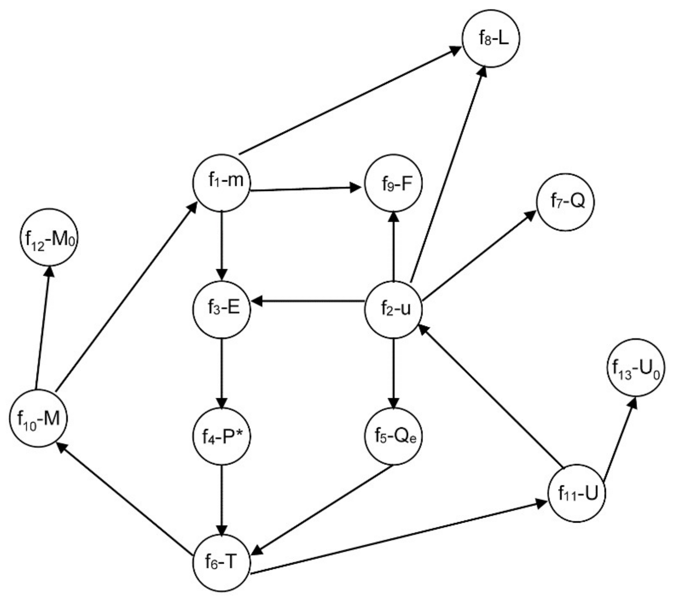
Each variable is assigned to the equation in which it is solved. Therefore, the system causality is {f1-m, f2-u, f3-E, f4-P*, f5-Qe, f6-T, f7-Q, f8-L, f9-F, f10-M, f11-U, f12-M0, f13-U0}. All this information is collected into an equation-variable directed graph where every node is labeled as “equation-variable”, as it is shown in Figure 3. An edge goes from node 1 to node 2, if node 2 computes a variable which also belongs to the equation of node 1.
Next, two examples are considered adding a new model assumption. These examples illustrate problems and contradictions that can arise with Hangos’ method.
3.2.1. Example 1: Removing Initial Conditions
Suppose that M is constant in the integral system of Equation (7), that is, the following assumption equation is added to the system:
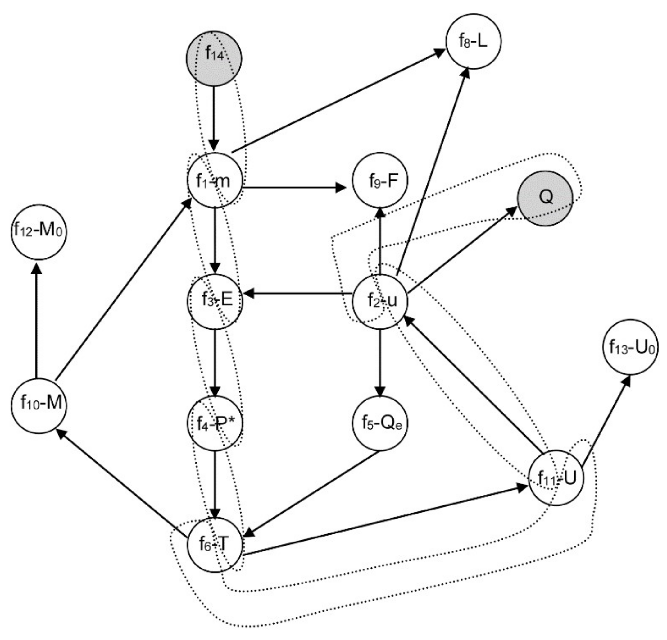
Each time the user adds a new equation, the graph is enlarged with a node. However, the system has zero degrees of freedom if the number of equations is equal to the number of unknowns. Hangos’ method proposes to remove equation f12 of (7) which is related with the initial condition of M0. Thus, the variable M0 is unassigned. This situation is illustrated in the equation-variable graph of Figure 4, where the modified nodes and the new nodes are filled in gray. The new causality assignment is {f1-E, f2-u, f3-P*, f4-T, f5-Qe, f6-M, f7-Q, f8-L, f9-F, f10-M0, f11-U, f13-U0, f14-m}. In the graph, the assignments changes are highilighted with ellipses in dashed line.
Hangos states that the system has a perfect matching; hence, the system differential index is one. Nevertheless, analyzing the new assignments, the following implications are obtained:
- From equation f14 (8), m = 0, and consequently, from f1 it is obtained that E is a function of F and L: E = F − L ⇒ E = E(F,L).
- Similarly, from equation f3 with P0 and kLV constant, P* is a function of F and L: .
- From f4, and assuming H invertible: .
- From f5 with T0 and qLV constant: .
- By equation f6 with ce and M constant: .
- Finally, from f2 with hF, hL, hLV constant: ⇒ .
Analyzing the last equation, the left side is a function of F and L design variables, and the right side only depends on Q, which is another design variable specified separately. Thus, a contradiction appears because the addition of Equation (8) makes the system over-constrained. To solve this new system, the number of equations must be the same as the number of unknowns. Therefore, another equation should be removed. Conversely, considering this system in a strict way, the initial conditions M0 and U0 are considered variables. If this integral system expects to be compatible with a differential one, the time derivatives of these two variables must be zero. Removing the equation f12: M0 = spec implies that the system from Example 1 does not satisfy M0′ = 0 and, therefore, this system is different from the original one.
3.2.2. Example 2: Removing an Arbitrary Specification Equation
Let us suppose that M is constant again; however, the equation f7 is selected to be removed from Equation (7). This is equivalent to relax the design variable Q, which means that the design variable Q turns into an unknown algebraic variable. The changed equation-variable assignments are given by: f14-m, f1-E, f3-P*, f4-T, f6-U, f11-u, f2-Q, as shown in Figure 5. Sorting the equations and highlighting the variables that are computed by each equation in square brackets, the new system can be written as in Equation (9).
Note that the system has a perfect matching, so Hangos’ method affirms that the system differential index is one. However, examining equation f11, the variable u is under integration. To isolate it, there are two alternatives:
- Derive equation f11. In this case, equations f13, f6, f10, f12, f4, f3, f1, f8 and f9 must also be derived. After that, a perfect matching is obtained and the index is two, contradicting the previous statement of index one.
- Solve integral f11 by a quadrature method. In this case, it can be thought that no derivative is necessary. However, applying some rules such as the trapezoidal rule, the following results are obtained:To decrease errors, these two formulas are subtracted:Solving the above integral by the trapezoidal rule:and isolating the term u(t + h), the following expression is achieved:The last expression is the numeric derivative of U(t), which shows that the system solution could not converge. Thus, this second alternative is not a good general alternative.
4. Proposed Method by Relaxation of Design Variables
From the examples of the previous section, it can be concluded that Hangos’ method is incomplete and needs to be improved. Modeling assumptions may induce changes in computational properties of the model and modifications in the variable-equation assignments. If the set of design variables is not changed properly, the index of the model can be increased or the zero degree of freedom will not be satisfied. In the next section, a modification of Hangos’ method is proposed. This modification relaxes a design variable for each new assumption equation and restores a system with zero degrees of freedom. Two kinds of model assumptions are considered: steady state equations and algebraic equations. First, the basis of the new procedure is introduced and exemplified. The effect of the model assumptions is described as a graph transformation acting on the structure graph of the model. Then, a new algorithm is proposed based on a graph approach and the fundamentals of this proposal are developed.
4.1. Basis of the Proposed Method
This section discusses how Hangos’ algorithm can be modified when a new algebraic or steady equation is introduced into the DAE system. The following notation is used:
- The capital letters (I, J, K, …) indicate design variables.
- The lowercase letters (a, b, c, …) denote the equation identifier and are placed to the left of the equation-variable node.
- The lowercase letters (u, v, w, …) represent system variables, which are placed to the right of the graph node. In particular, x and s are states and u, v and w denote algebraic variables.
- An arrow marked with an asterisk indicates that there is a path from the first node to the last one.
To restore the property of zero degrees of freedom after adding a new equation, it is proposed to reduce in one the number of design variables specified by the user, that is relaxing a design variable by removing its corresponding specification equation. After this modification, two vertices of the associated graph remain without matching edges and a new assignment can be constructed starting from the previous one. This minimizes the analysis time, making the modeling tool even more responsive to the user. Then, a closest maximum assignment is performed. This assignment has the largest number of matching edges in common with the original full assignment.
4.1.1. Steady Equation Addition
When a state variable is assumed at steady state, a new equation d is added with the form d: x′ = 0. To relax a design variable, there are two possibilities: connecting the new equation d with the selected design variable I with a straight path, or linking the equation through a state variable s.
In the first case, connecting the new equation with the design variable with a straight path (Figure 6a), the new causality assignment is completed by combining every equation with a variable of the next one and combining the last equation with the design variable I, as shown in Figure 6b. The final assignment causality is shown in Figure 6c. Note that this new system has a differential index of one.
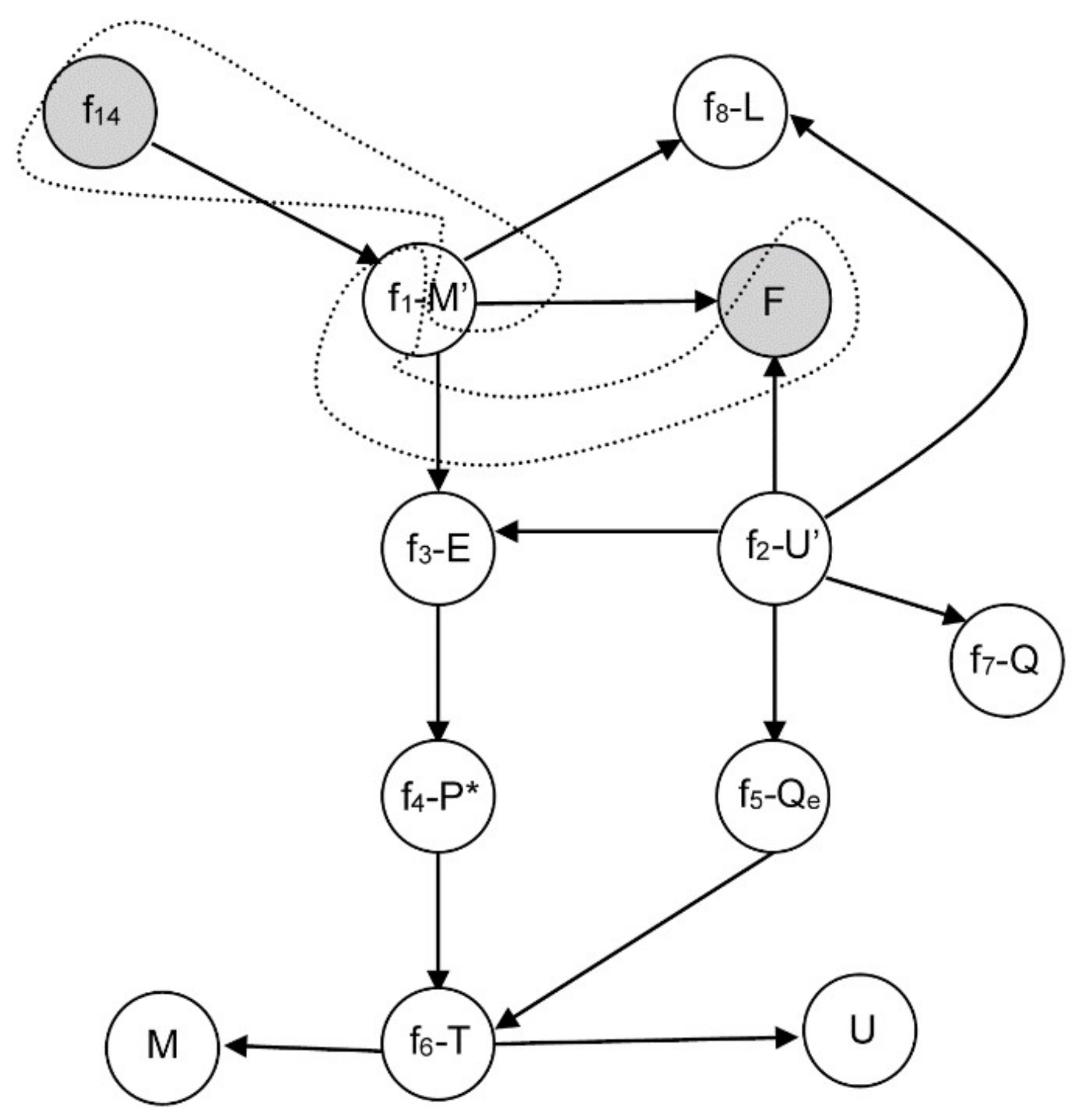
For instance, let suppose again that the assumption equation f14 in (8) is added to the original DAE system in (6) in the process example of Section 3.2. The original set of equation is preferred instead of the integral one proposed by Hangos in (7), in order to avoid possible inconsistency problems. The selected design variable to relax is F, so the specification equation f9 is removed from (6). In this case, there is a direct path from f14 to F. Figure 7 shows the causality assignment of the initial system in the corresponding equation-variable graph and the changed causality assignments of the modified system which are represented by dotted lines. The new causality assignment is {f14-M′, f1-F, f2-U′, f3-E, f4-P*, f5-Qe, f6-T, f7-Q, f8-L}.
The second possibility consists of linking equation d indirectly with the selected design variable I through the state variable s, see Figure 8. There is a differential edge from node s to node c-s′ represented as a dashed arrow. In this case, an index reduction algorithm, such as Pantelides’ algorithm [10], must be applied. This algorithm shows that the path from d to node s must be derived. Equations involved in this path must also be derived. The new system causality is shown in Figure 8c. Thus, in this situation, the differential index is higher than one.
Consider again the previous example of Section 3.2 and suppose now that the selected design variable to relax is Q. Then, the specification equation f7 is removed. The path from equation f14 to variable Q is shown in Figure 9. Note that there is a differential edge from node U to node f2-U′. After applying Pantelides’ algorithm to reduce the differential index of the system, the new causality assignment is {f14-M′, f1-E, f3-P*, f4-T, f6-U, f′10-M′′, f′1-E′, f′3-P*′, f′4-T′, f′6-U′, f2-Q, f5-Qe, f8-L, f9-F}. The variables are classified as state (M), derivative (M′) and algebraic (E, Q, P*, T, Qe, U, U′, M′′, E′, P*′, T′). The new system has zero degrees of freedom, a perfect matching and a differential index of one. Thus, the original system has a differential index of two.
4.1.2. Algebraic Equation Addition
Suppose that an algebraic equation d is added to the DAE system with the form d: z = constant. In this situation, the same alternatives as those of previous subsections are found. Figure 10 shows a straight path from d to design variable I and the new causality assignment. Note that the final system has a perfect matching.
In the second case, equation d is linked with a design variable I by a path through a state variable s (Figure 11). To obtain a perfect matching, it is necessary to apply an index reduction algorithm, such as Pantelides’ algorithm, as shown in Figure 11c. Therefore, in this example, the differential index of the system is two.
4.1.3. General Case
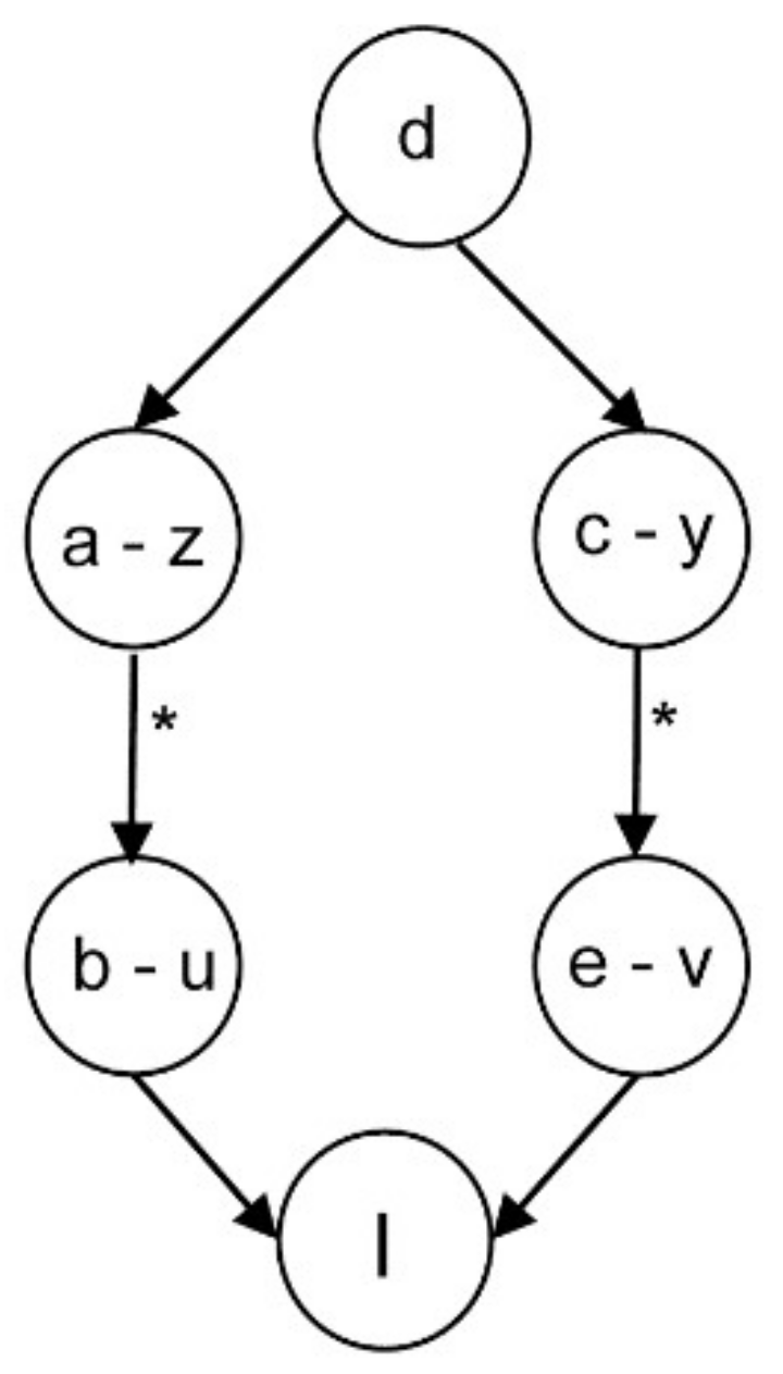
The most general assumption appears when an equation with several algebraic variables is added. In this case, it is enough to find a link from any of the paths that begin at vertex d to the selected design variable I. As an example, let us suppose that the equation d is added with the form d: z = y. In Figure 12, two alternatives for finding the design variable that solves this problem are shown.
4.2. Proposed Algorithm
The suggested procedure is generalized in the proposed Algorithm 2, that relates algebraic and state variables in the assumption equations with design variables through straight paths or through the state variables of the initial system. This algorithm allows the addition of several equations simultaneously and tries to maintain the highest number of intact equation-graph associations of the initial system as possible, that is, the closest assignment. The algorithm can be combined with another index reduction algorithm to solve the causality assignment in one step. In comparison with the Hangos’ Algorithm 2, discussed in Section 2.1, the proposal offers some improvements that optimize its computational cost and behavior. Since a maximum weight matching of a bipartite graph can be calculated in polynomial time [27], the closest assignment problem has the same time bound as valid.
A first improvement concerns the weight function w in (5) used by Hangos. It will be proven that there is a family of functions which obtain the same solution as the w in (5) and that they are simpler to compute.
Definition 1.
Let a and b be two real numbers with a > b. Let B(L, R, E) be a bipartite graph with a matching F. We define the weight function wab as
Lemma 1.
Let a and b , with a > b. Let B(L, R, E) be a bipartite graph with a matching F and weight function wab. Let M be the maximum matching of maximum weight and M′ be any other maximum matching, then .
Proof.
Because M and M′ are maximum matchings: |M| = |M′| and |M ∩ F| + |M ∩ Fc| = |M′ ∩ F| + |M′ ∩ Fc|. Then:
|M ∩ F| − |M′ ∩ F| = |M′ ∩ Fc| − |M ∩ Fc|.
Because wab(M) ≥ wab(M′) ⇒ ⇒ a|M ∩ F| + b|M ∩ Fc| ≥ a|M′ ∩ F| + b|M′ ∩ Fc|. By arranging all of the expressions to the left-hand side and gathering the expressions that are preceded by a or b, it follows:
a(|M ∩ F| − |M′ ∩ F|) + b(|M ∩ Fc| − |M′ ∩ Fc|) ≥ 0.
By (15), the following relation is deduced:
a(|M ∩ F| − |M′ ∩ F|) − b(|M ∩ F| − |M′ ∩ F|) ≥ 0.
This implies:
(a − b)(|M ∩ F| − |M′ ∩ F|) ≥ 0.
Because a > b, the expression of the first bracket is a positive number. Therefore, the proposed result is obtained. ☐
From Lemma 1, any wab function can be selected to obtain a maximum matching of maximum weight M, which has the maximum number of element shared with F, considering the set of maximum matchings, that is: M′ ∈ {M′′/M′′ is a maximum matching} ⇒ |M ∩ F| ≥ |M′ ∩ F|.
Theorem 4.
Let a, b, c and d ∈ ℜ, such that a > b and c > d. If we let B(L, R, E) be a bipartite graph with a matching F, then M is a maximum matching of maximum weight with wab if and only if M is a maximum matching of maximum weight with wcd.
Proof.
⇒ It is assumed that M is a matching of maximum weight for wab, and it will be proven that this is also true for wcd. Let M′ be any maximum matching, and by Lemma 1:
By multiplying (19) by c − d, c > d, we obtain: , and therefore:
Because M and M′ are maximum matchings, it follows:
By arranging (21):
By replacing (22) into (20), it follows:
This implies that
⇐ This result is obtained in a similar manner. ☐
Theorem 4 allows taking any wab function as a weight function, with a > b. The simplest function of this family is the characteristic function of the matching F, which is :
As a consequence of Theorem 3, taking a matching of maximum weight in a run, another matching of maximum weight is in the next run. Therefore, if F is considered initially, then the number of iterations is drastically reduced.
The next proposition characterizes a maximum matching of maximum weight regarding to the initial matching F.
Lemma 2.
Let B(L, R, E) be a bipartite graph. Let F and M be two matching with |M| > |F|. If |M ∩ F| is the maximum among all matchings with cardinality |M|, then M ∆F has neither cycles nor alternating paths with even lengths.
Proof. (by contradiction)
Suppose for the sake of contradiction that M ∆ F has cycles or alternating paths with even lengths.
- (1)
- M ∆ F is decomposed into , where:
- All of the sets pi, di and ci are disjointed.
- pi represents the augmented paths in F. There are k = |M| − |F| > 0 paths of this kind, and all of them have odd length. Moreover, the number of edges of pi in F + 1 is equal to number of edges of pi in M − F, that is:|pi ∩ F| + 1 = |pi ∩ (M − F)| = (|pi| + 1)/2.
- di represents an alternating path of even length. The number of edges of di in F is equal to the number of edges of di in M − F:|di ∩ F| = |di ∩ (M − F)| = |di|/2.
- ci represents cycles, and therefore, their length is even. They fulfill the same equation as di, that is:|ci ∩ F| = |ci ∩ (M − F)| = |ci|/2.
- (2)
- Let M′ = F ∆ (). If M′ is a matching in B and its cardinality is , then:In contrast,
- (3)
- According to our hypothesis, if |M ∩ F| is maximum among all the matchings of cardinality |M|, then: |M ∩ F| |M′ ∩ F|. By (29) and (30):Equation (31) can be simplified to:By replacing the Expressions (27) and (28) into (32):This expression implies that:which is a contradiction. ☐|di| = 0 ∀ i = 1, …, r and |ci| = 0 ∀ i = 1, …., s,
Theorem 5.
Let B(L, R, E) be a bipartite graph. Let F be a matching of B and wF, the characteristic function of F. Let M be a maximum matching of maximum weight for wF. If , then there are k augmented paths disjoined by vertexes {p1, …, pk} in F, such that:
- 1.
- M = F ∆ p1 ∆… ∆ pk.
- 2.
- .
- 3.
- .
Proof.
- It is known by Lemma 1 that the cardinality of M ∩ F is the maximum among all the maximum matchings. After applying Lemma 2, the desired result is obtained.
- By (26) and (29) of Lemma 2, it follows that:
- By the last expression:As k = |M| − |F|, then:
The above theorem states the relation between the cardinals of the augmented path of F, F itself and the maximum matching of maximum weight M.
Corollary 1.
Under the assumptions of Theorem 5, is the lowest among all the sums of any k vertex-disjoint augmenting paths of F.
Proof.
Let {q1, …, qk} be any k vertex-disjoint augmenting paths of F. The matching M′ = F ∆q1 ∆ … ∆qk has a cardinality of |M′| = |F| + k = |M|. By applying Theorem 5 we deduce that:
In contrast:
By Lemma 1: |M ∩ F| |M′ ∩ F| and by the relations (38) and (39), then:
By operating in the last expression, we deduce that . ☐
Using the previous results, the Algorithm 2 is proposed. It is based on the construction of assignments using graph theory and the Algorithm 1 of Section 2, and is an improvement of Hangos’ Algorithm 2. The algorithm expects as input a bipartite graph B(L, R, E) representing the system equations, the weight function w such as that in (25), and an initial matching F before adding modeling assumptions. The complexity to compute the maximum matching starting from an empty matching is O(V·E); however, it is reduced to O(E) when the graph is enlarged by adding only one new node and a previous maximum matching is already known [20]. This algorithm uses the information generated in previous steps of the simulation, so the initial matching F is not discarded, which is an improvement over algorithms that need to start from scratch (these kinds of algorithms have a cost O(V2 + V·E)). This can make the modeling tool more responsive to user specification changes.
If Q is the number of assumption equations, the time complexity varies depending on the algorithm used in the computation of the path of the lowest cost in GM (step 3.1). When the Bellman-Ford algorithm is employed, the overall time cost is polynomial with O(Q·V·E), since it is performed one time for each new assumption added to the system.
| Algorithm 2. Find the maximum matching such that |M ∩ F| is highest. |
| Input: A bipartite graph B(L, R, E), weight function w and initial maximum matching F. Output: Matching of maximum weight closest to F. 1: M := F 2: Construction of a direct graph GM (V, EM) with function weight z. 2.1: V = L ∪ R 2.2: EM is defined by: If the undirected edge (l, r) ∈ Mc then the directed edge (l, r) ∈ EM. else if the undirected edge (l, r) ∈ M then the directed edge (r, l) ∈ EM. end if That is, the set of edges EM is: EM = {(l, r)/(l, r) ∈ Mc} ∪ {(r, l)/(l, r) ∈ M} 2.3: The weight function z is defined: If (l, r) ∈ EM then z(l, r) = w (l, r). else if (r, l) ∈ EM then z(r, l) = − w((l, r) end if 2.4: Append a new vertex s linked to all free vertexes of L. 2.5: Append a new vertex t which is the destination of all free vertexes of R. 3: while there exists an augmented path p into GM do 3.1: p = an augmented path of lowest cost in GM 3.2: M := M ∆ p 3.3: Adjust GM by path p. end while |
The cost of the algorithm can also be improved if it is noted that the edges of GM can take only values from the set {−1, 0, 1}. In [26], the authors proposed an algorithm based on Dijkstra’s algorithm with linked list or minimal heaps that improves the time complexity of algorithm 1. This algorithm can be used if the weight of the edges is a positive integer in the range {0, 1, 2, …, W}, where W is the highest value of any edge. To apply this algorithm to the proposed one, it is necessary to reduce the set {−1, 0, 1} of the weight function in (25) to a set of a positive integers. The next theorem resolves this limitation.
Theorem 6.
Let G(V, E) be a graph with weight function w and let k be any real number. Then, M is a matching of maximum weight among all matchings of cardinality |M| for w ⇔ M, which is a matching of maximum weight among all the matchings of cardinality |M| for w2 = w + k.
Proof.
Let M′ be a matching of cardinality |M|. According to our hypothesis, w(M) ≥ w(M′), so:
According to (25), the weight function w of graph GM only takes on values in the set {−1, 0, 1}. By applying Theorem 6 for k = 1, the problem is reduced to another one where the values of the weight function belong to the set {0, 1, 2}. Thus, Dijkstra’s algorithms can be applied to step 3.1 of the proposed algorithm. Using the Dijkstra’s algorithm with minimal heaps, the time complexity is O(Q·(E + V·log(V))). When the Dijkstra’s algorithm is implemented with linked list, the overall time cost is reduced to O(Q·(V + E)) [22]. In this last case, the algorithm is almost linear because Q is supposed to be small. Therefore, if the cardinality of Q is negligible against V + E, the cost is O(V + E).
5. Conclusions
Often the system under study is described by a system of DAEs. These equations are usually parameterized by the design variables, which are known during the simulation. If a new assumption equation is added to the system, it becomes over-constrained. There are several methods to reduce the new system to a well-constrained one, such as Hangos’ method. This method basically consists of removing an equation from the original system to equal the number of equations and variables. However, this procedure requires that the new system contradicts the first one and, in some cases, the solution of the transformed system is far from one which describes the initial system. This paper presented an alternative to Hangos’ method which preserves the original formulation of the system. The basis of this new method is to relax design variables, converting them into new algebraic variables. This procedure achieves a solution compatible with that of the initial system.
The example proposed in [21] has been studied with a simulation of a reactor with input and output flows. The differential system has been transformed into an integral one, as Hangos’ method shows. Then, a new assumption equation has been added and a new system that is not related to the first one has been obtained. However, by applying the method suggested by the authors, an accurate system with the initial equations is obtained.
Also, an algorithm has been developed based on graph theory, starting from the initial matching of equation-variables. This algorithm has the followings characteristics:
- It relates algebraic and state variables of the assumptions equations to the design variables of the system selected by the user.
- It allows the addition of several assumption equations and obtaining a greater number of common edges with the starting system.
- In the best case, depending on the implementation, the computational cost is O(Q(E + V)), where Q is the number of assumption equations, V the number of vertexes in the bipartite equation-variable graph and E is the number of edges in that graph. Therefore, if the number of assumption equations is small, the cost of the algorithm is linear.
- The algorithm can be combined with an algorithm of index reduction.
Author Contributions
Antonio Belmonte and Juan Garrido conceived and design the method; Jorge E. Jiménez and Francisco Vázquez analyzed the method; and Francisco Vázquez and Juan Garrido wrote the paper.
Conflicts of Interest
The authors declare no conflict of interest.
References
- Garrido, J.; Zafra, A.; Vazquez, F. Object oriented modelling and simulation of hydropower plants with run-of-river scheme: A new simulation tool. Simul. Model. Pract. Theory 2009, 17, 1748–1767. [Google Scholar] [CrossRef]
- Nikolić, D.D. Dae tools: Equation-based object-oriented modelling, simulation and optimisation software. PeerJ Comput. Sci. 2016, 2, e54. [Google Scholar] [CrossRef]
- Fritzson, P.; Engelson, V. Modelica—A Unified object-oriented language for system modeling and simulation. In ECOOP’98—Object-Oriented Programming; Springer: New York, NY, USA, 1998; pp. 67–90. [Google Scholar]
- Piela, P.; Epperly, T.; Westerberg, K.; Westerberg, A. Ascend—An object-oriented computer environment for modeling and analysis—The modeling language. Comput. Chem. Eng. 1991, 15, 53–72. [Google Scholar] [CrossRef]
- Vázquez, F.; Jiménez, J.; Garrido, J.; Belmonte, A. Introduction to Modelling and Simulation with Ecosimpro; Pearson Educacion: Madrid, Spain, 2010; p. 272. [Google Scholar]
- Brenan, K.E.; Campbell, S.L.; Petzold, L.R. Numerical Solution of Initial-Value Problems in Differential-Algebraic Equations; Society for Industrial and Applied Mathematics: Philadelphia, PA, USA, 1996. [Google Scholar]
- Navarro, A.; Vassiliadis, V. Computer algebra systems coming of age: Dynamic simulation and optimization of dae systems in mathematica™. Comput. Chem. Eng. 2014, 62, 125–138. [Google Scholar] [CrossRef]
- Cellier, F.E.; Kofman, E. Continuous System Simulation; Springer Science & Business Media: Berlin, Germany, 2006. [Google Scholar]
- Tarjan, R. Depth-first search and linear graph algorithms. SIAM J. Comput. 1972, 1, 146–160. [Google Scholar] [CrossRef]
- Pantelides, C.C. The consistent initialization of differential-algebraic systems. SIAM J. Sci. Comput. 1988, 9, 213–231. [Google Scholar] [CrossRef]
- Cafferkey, N.; Provan, G. An analysis of performance-critical properties of modelica models. IFAC-PapersOnLine 2015, 48, 210–215. [Google Scholar] [CrossRef]
- Unger, J.; Kroner, A.; Marquardt, W. Structural-analysis of differential-algebraic equaion systems—Theory and applications. Comput. Chem. Eng. 1995, 19, 867–882. [Google Scholar] [CrossRef]
- Hangos, K.; Cameron, I. A formal representation of assumptions in process modelling. Comput. Chem. Eng. 2001, 25, 237–255. [Google Scholar] [CrossRef]
- Merchan, V.; Esche, E.; Fillinger, S.; Tolksdorf, G.; Wozny, G. Computer-aided process and plant development. A review of common software tools and methods and comparison against an integrated collaborative approach. Chem. Ing. Tech. 2016, 88, 50–69. [Google Scholar] [CrossRef]
- Jensen, A.K. Generation of Problem Specific Simulation Models within an Integrated Computer Aided System; CAPEC-DTU: Lyngby, Denmark, 1998. [Google Scholar]
- Bogusch, R.; Lohmann, B.; Marquardt, W. Computer-aided process modeling with modkit. Comput. Chem. Eng. 2001, 25, 963–995. [Google Scholar] [CrossRef]
- Moe, H.I. Dynamic Process Simulation: Studies on Modeling and Index Reduction. Ph.D. Thesis, University of Trondheim, Trondheim, Norway, 1995. [Google Scholar]
- Murota, K. Systems analysis by graphs and matroids. Structural solvability and controllability. SIAM Rev. 1989, 31, 502. [Google Scholar]
- Leitold, A.; Hangos, K. Structural solvability analysis of dynamic process models. Comput. Chem. Eng. 2001, 25, 1633–1646. [Google Scholar] [CrossRef]
- Soares, R.D.P.; Secchi, A.R. Structural analysis for static and dynamic models. Math. Comput. Model. 2012, 55, 1051–1067. [Google Scholar] [CrossRef]
- Hangos, K.; Szederkenyi, G.; Tuza, Z. The effect of model simplification assumptions on the differential index of lumped process models. Comput. Chem. Eng. 2004, 28, 129–137. [Google Scholar] [CrossRef]
- Cormen, T.H.; Leiserson, C.E.; Rivest, R.L.; Stein, C. Introduction to Algorithms, 2nd ed.; McGraw-Hill: New York, NY, USA, 2001. [Google Scholar]
- Korte, B.; Vygen, J.; Korte, B.; Vygen, J. Combinatorial Optimization; Springer: Berlin, Germany, 2012; Volume 2. [Google Scholar]
- Tassa, T. Finding all maximally-matchable edges in a bipartite graph. Theor. Comput. Sci. 2012, 423, 50–58. [Google Scholar] [CrossRef]
- Micali, S.; Vazirani, V.V. An O(v|v| c |E|) algorithm for finding maximum matching in general graphs. In Proceedings of the 21st Annual Symposium on Foundations of Computer Science, Syracuse, NY, USA, 13–15 October 1980; pp. 17–27. [Google Scholar]
- Gabow, H.N.; Tarjan, R.E. Faster scaling algorithms for general graph matching problems. J. ACM 1991, 38, 815–853. [Google Scholar] [CrossRef]
- Hopcroft, J.E.; Karp, R.M. An n^5/2 algorithm for maximum matchings in bipartite graphs. SIAM J. Comput. 1973, 2, 225–231. [Google Scholar] [CrossRef]
- Mucha, M.; Sankowski, P. Maximum matchings via gaussian elimination. In Proceedings of the 45th Annual IEEE Symposium on Foundations of Computer Science, Rome, Italy, 17–19 October 2004; pp. 248–255. [Google Scholar]
- Goel, A.; Kapralov, M.; Khanna, S. Perfect matchings in O(n\logn) time in regular bipartite graphs. SIAM J. Comput. 2013, 42, 1392–1404. [Google Scholar] [CrossRef]
- Frenkel, J.; Kunze, G.; Fritzson, P. Survey of appropriate matching algorithms for large scale systems of differential algebraic equations. In Proceedings of the 9th International MODELICA Conference, Munich, Germany, 3–5 September 2012; Linköping University Electronic Press: Linköping, Sweden, 2012; pp. 433–442. [Google Scholar]
- Berge, C. Two theorems in graph theory. Proc. Natl. Acad. Sci. USA 1957, 43, 842–844. [Google Scholar] [CrossRef] [PubMed]
- Har-Peled, S. Matchings II. Available online: https://courses.engr.illinois.edu/cs473/fa2015/w/lec/lec/31_matchings_II.pdf (accessed on 8 April 2018).
Figure 1.
A bipartite graph (a) and the corresponding directed graph (b).
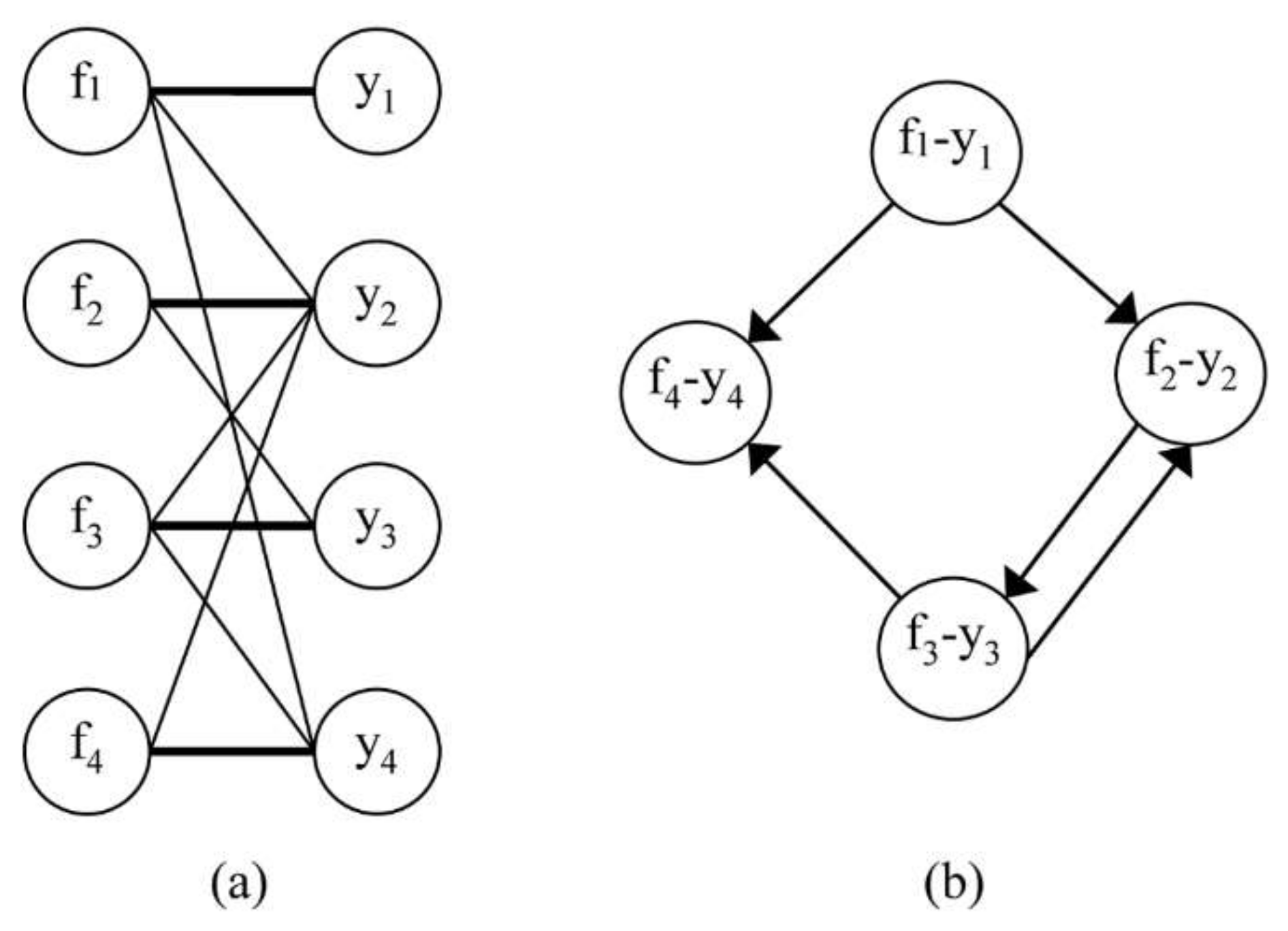
Figure 2.
Open evaporator.
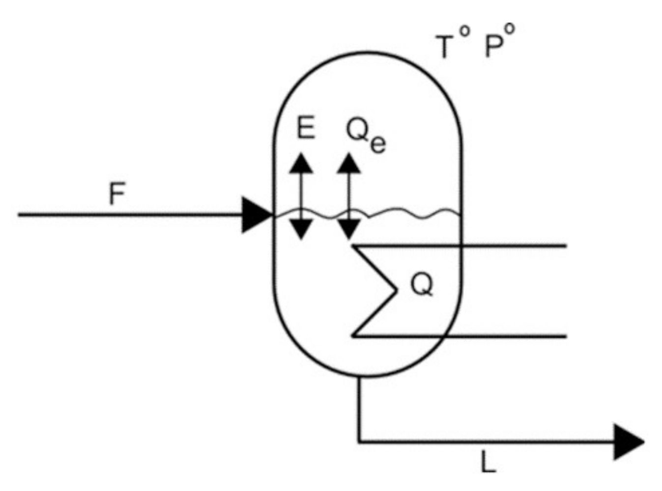
Figure 3.
Equation-variable graph of system (7).

Figure 4.
Equation-variable graph under condition m = 0.

Figure 5.
Equation-variable graph with the new causality assignment relaxing variable Q.

Figure 6.
Equation d linked with variable I with a straight path (a); matching problem (b) and final causality assignment (c).
Figure 6.
Equation d linked with variable I with a straight path (a); matching problem (b) and final causality assignment (c).
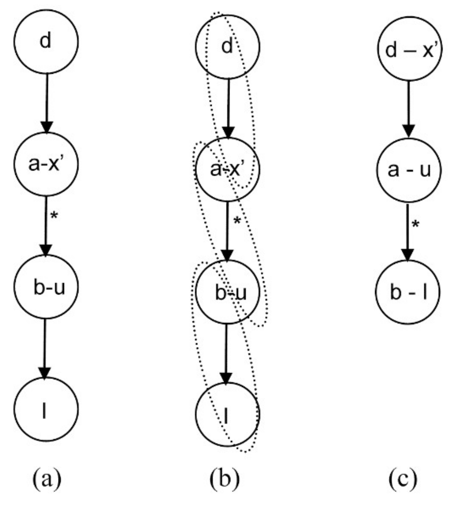
Figure 7.
Causality assignment after relaxing F.

Figure 8.
Equation d linked to variable I through a differential path (a), and causality assignments before path derivation (b) and after derivation with differential index of two (c).
Figure 8.
Equation d linked to variable I through a differential path (a), and causality assignments before path derivation (b) and after derivation with differential index of two (c).
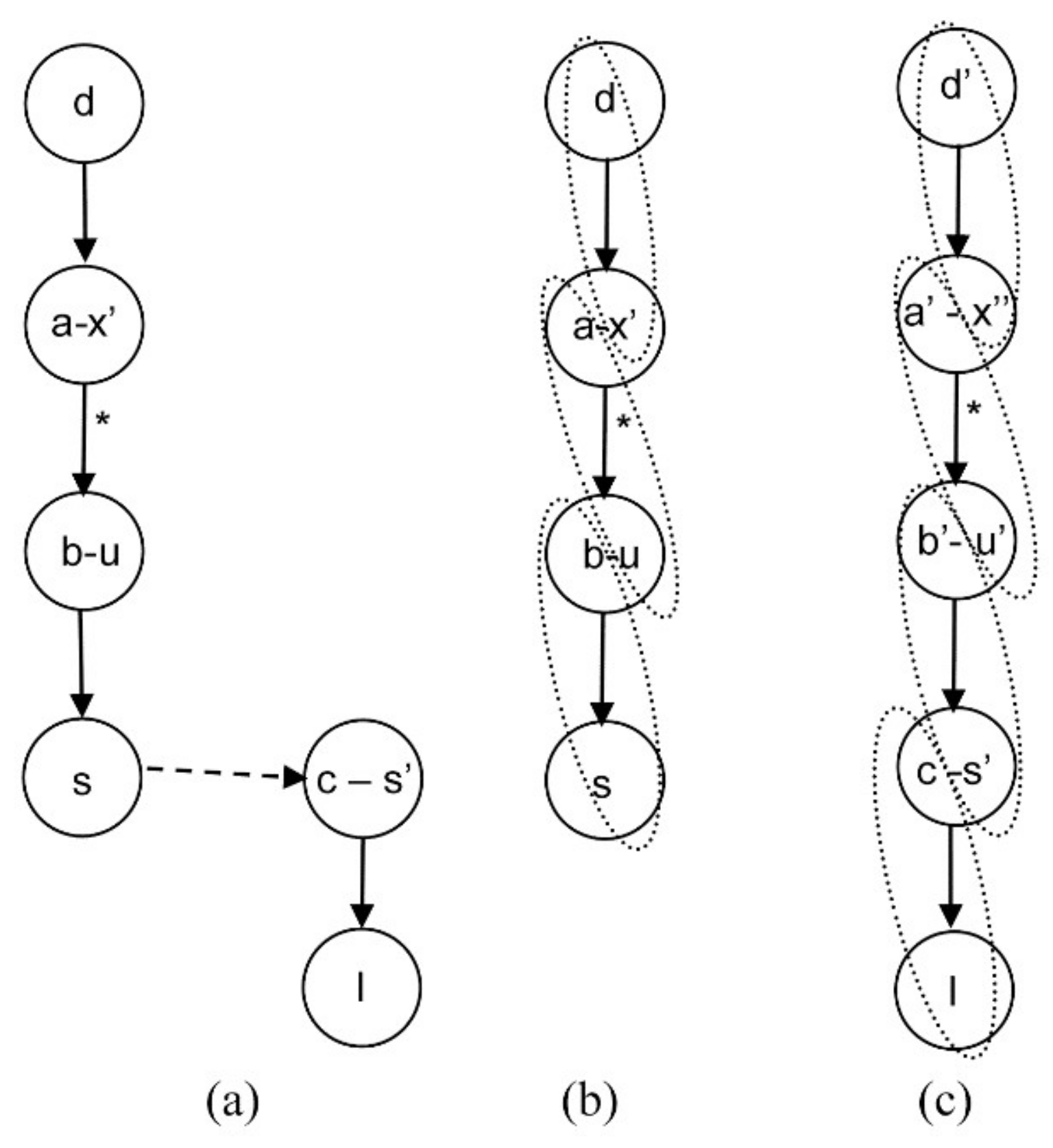
Figure 9.
Causality assignment after relaxing Q.

Figure 10.
Linking equation d to design variable I by a straight path (a); and solution of the assignment problem (b).
Figure 10.
Linking equation d to design variable I by a straight path (a); and solution of the assignment problem (b).

Figure 11.
Equation d linked with design variable I through the state variable s (a), and causality assignments before path derivation (b) and after derivation with differential index of two (c).
Figure 11.
Equation d linked with design variable I through the state variable s (a), and causality assignments before path derivation (b) and after derivation with differential index of two (c).
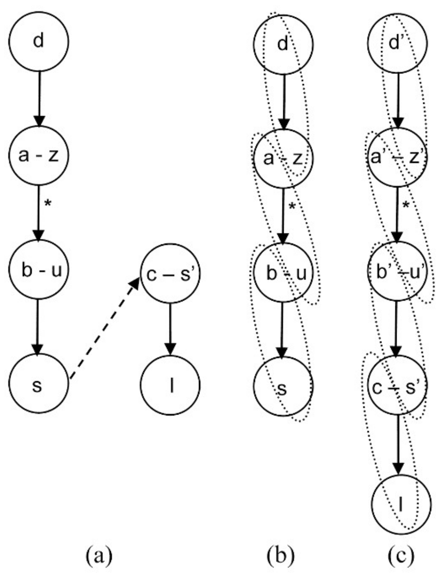
Figure 12.
Several paths linking with the design variable I.
© 2018 by the authors. Licensee MDPI, Basel, Switzerland. This article is an open access article distributed under the terms and conditions of the Creative Commons Attribution (CC BY) license (http://creativecommons.org/licenses/by/4.0/).
Share and Cite
MDPI and ACS Style
Belmonte, A.; Garrido, J.; Jiménez, J.E.; Vázquez, F. Recomputing Causality Assignments on Lumped Process Models When Adding New Simplification Assumptions. Symmetry 2018, 10, 102. https://doi.org/10.3390/sym10040102
AMA Style
Belmonte A, Garrido J, Jiménez JE, Vázquez F. Recomputing Causality Assignments on Lumped Process Models When Adding New Simplification Assumptions. Symmetry. 2018; 10(4):102. https://doi.org/10.3390/sym10040102
Chicago/Turabian StyleBelmonte, Antonio, Juan Garrido, Jorge E. Jiménez, and Francisco Vázquez. 2018. "Recomputing Causality Assignments on Lumped Process Models When Adding New Simplification Assumptions" Symmetry 10, no. 4: 102. https://doi.org/10.3390/sym10040102
Note that from the first issue of 2016, this journal uses article numbers instead of page numbers. See further details here.