Stability of Bounded Dynamical Networks with Symmetry

ESIPP, University College Dublin, Dublin 4, Ireland
Symmetry 2018, 10(4), 121; https://doi.org/10.3390/sym10040121
Submission received: 2 April 2018
/
Revised: 12 April 2018
/
Accepted: 13 April 2018
/
Published: 19 April 2018
Abstract
:Motivated by dynamical models describing phase separation and the motion of interfaces separating phases, we study the stability of dynamical networks in planar domains formed by triple junctions. We take into account symmetry, angle-intersection conditions at the junctions and at the points at which the curves intersect with the boundary. Firstly, we focus on the case of a network where two triple junctions have all their branches unattached to the boundary and then on the case of a network of hexagons, with one of them having all its branches unattached to the boundary. For both type of networks, we introduce the evolution problem, identify the steady states and study their stability in terms of the geometry of the boundary.
MSC:
70K20; 70K701. Introduction
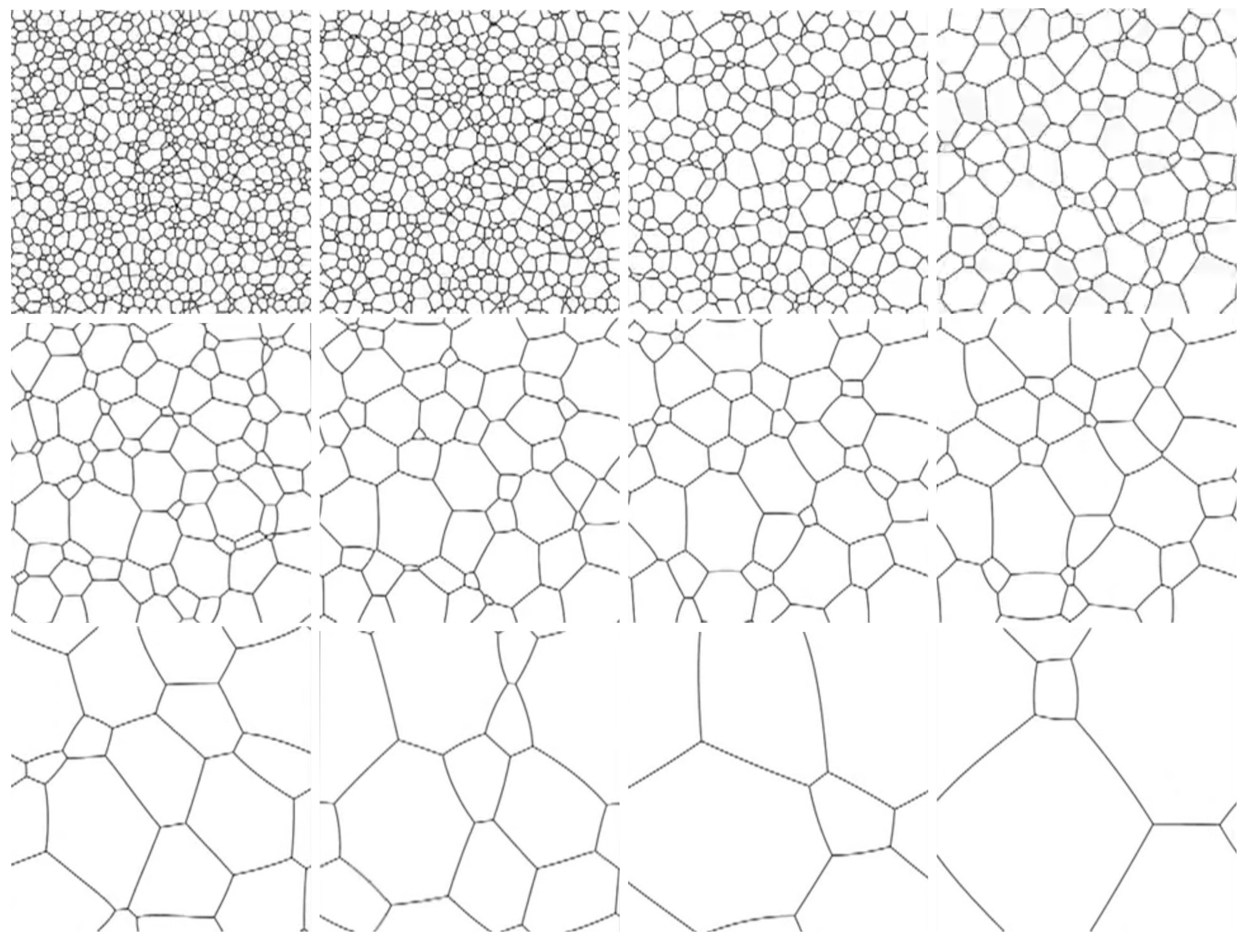
The study of the geometric evolution problem of dynamical networks in planar domains formed by triple junctions has always been very important in the modelling of many phenomena in various fields of science, physics and engineering; see [1,2,3]. In Figure 1, we see the evolution of such a network; see also [4].
In many cases, this type of dynamical network forms hexagonal networks. The hexagon is the highest-sided tessellate regular polygon; see [5]. This makes it uniquely important in a variety of fields, since it has the advantage of spacing out each constituent hexagon more or less evenly from its neighbours. Common examples of this use of hexagonal cells can be found in such varied fields as cellular automaton, statistical sampling, board games, computer games, the comb of the esteemed honeybee, and so on; see [5,6]. Hence, we see hexagonal dynamical networks in several evolution problems in nature like polycrystalline camphor-ethanol mixture, soap bubbles and honeycombs; see Figure 2.
About 20 years ago, motivated by dynamical models in material science describing phase separation and the motion of interfaces’ separating phases, Bronsard et al. [7,8,9,10] introduced the problem of networks of curves in a planar domain with normal velocity proportional to the curvature and fixed angle conditions at the point at which the curves intersect. From the underlying model, they derived the equations of motion, as well as the boundary conditions. The angles formed by the curves at a node are constant throughout the evolution and intersect the boundary of the domain orthogonally at all times. Our interest is in studying a network of curves that is in motion, with the normal velocity equal to the curvature. Note that Freire (see [11]) has considered similar graphs over a bounded domain in , intersecting along a time-dependent curve and moving by mean curvature while preserving the pairwise angles at the curve of intersection (equal to ). For the corresponding two-dimensional parabolic free boundary problem, he proved the short-time existence of classical solutions, for sufficiently regular initial data satisfying a compatibility condition.
For some recent contributions, see [12,13,14] and the references therein. For recent applications using the mathematics of networks, see [15,16,17,18]. Some common results with graph theory can be found in [19,20,21,22,23].
A network of three curves that intersect at a node is the simplest case. This case, as well as the cases of a network of two triple junctions and a hexagonal network with one hexagon have been studied in [24,25].
1.1. Problem Formulation
Mathematically, a bounded dynamical network of m curves can be formulated as follows. Let be a bounded domain. Consider the increasingly-smooth functions , satisfying . For each , let:
Be smooth functions such that is an embedding describing the curve i contained in ; is time, s, , the arc length parameter. The evolution of is described by:
Subject to the following conditions:
- Incidence conditions: A curve i has two ends at and at .
- (a)
- If at the point , curve i intersects with two other curves, namely curves j and q, at their starting point for example, then:Then, at the other end of curve i, at point , curve i intersects:
- with two other curves, namely curves p and r at their ending points:or,
- at the boundary :where is a real function of two variables that describes locally the boundary .
- (b)
- If at the point , curve i intersects with the boundary instead of two other curves, then:In this case, at the other end of curve i, at point , curve i intersects with two other curves, namely curves p and r, at their ending point:
- Angle conditions:
- (a)
- At the point at which the curves intersect: If curves intersect at their starting points, for example, then:
- (b)
- At :
where , , and is the Euclidean inner product.
Remark 1.
are embeddings in the plane, and the network is in motion with the normal velocity equal to the curvature law:
is the normal velocity of the curve ; is the unit normal vector to ; = is the unit tangent vector; and the vector (, ) has the orientation of the coordinate system, which is valid locally.
Remark 2.
is the tangential velocity of curve and the curvature of curve . Moreover, the velocity of the curve i is given by:
or, equivalently,
Note that , because is perpendicular to , and thus:
or, equivalently,
1.2. Changing the Domain
It would be more convenient to formulate the problem in a way that the arc length parameter s takes its values in a domain independent of time t. For this purpose, let:
and:
with , and . Then:
Furthermore:
or, equivalently,
or, equivalently,
The system of equations (1) will then take the form:
and will be defined in the set = . Let , be the tangent and normal vector, respectively, of curve i. Then, by multiplying the above expression by , we get:
or, equivalently, by taking into account that :
The tangential term in the equation can be assigned at will without affecting the equations . Thus, the m equations that are compatible with motion by curvature are the following:
Equations (2) have to be supplemented with the conditions of (1), which will take the following form:
- Incidence conditions: A curve i has two ends at and at .
- (a)
- If at the point , curve i intersects with two other curves, namely curves j and q, at their starting points for example, then:Then, at the other end of curve i, at point , curve i intersects:
- with two other curves, namely curves p and r, at their ending points for example:or,
- at the boundary :
- (b)
- If at the point , curve i intersects with the boundary instead of two other curves then:In this case, at the other end of curve i, at point , curve i intersects with two other curves, namely curves p and r, at their ending points for example:
- Angle conditions:
- (a)
- At the point at which the curves intersect: If curves intersect at their starting point for example, then:
- (b)
- at :
The condition is not sufficient by itself to determine the evolution. Different equations for the embedding are expected to lead to different evolutions for the curves in which the nodes do not affect the evolution.
1.3. Stability
In this subsection, we present the eigenvalue problem related to the equations of (2) in order to study the stability of the steady states. We define the family of perturbations :
where , are real-valued functions of class and is the length of curve . If is the curvature of curve i, then from the Frenet formulas and [25,26,27], , we obtain the following eigenvalue problem:
The conditions of (2) will take the following form:
- Incidence conditions: A curve i has two ends at and at .
- (a)
- If at the point , curve i intersects with two other curves, namely curves j and q, at their starting points for example, then:Then, at the other end of curve i, at point curve i intersects:
- with two other curves, namely curve p and r, at their ending points for example:or,
- at the boundary :
- (b)
- If at the point , curve i intersects with the boundary instead of two other curves, then:In this case, at the other end of curve i, at point , curve i intersects with two other curves, namely curves p and r, at their ending points for example:
- Angle conditions:
- (a)
- At the point at which the curves intersect: If curves intersect at their starting points for example, then:
- (b)
- at :
The following Lemma has been proven in [25].
Lemma 1.
If , and , then
2. A Bounded Network with Two Inner Triple Junctions
We will begin the section with the following definition:
Definition 1.
A junction of a network inside a bounded domain will be called an internal junction if all its branches have their ends unattached to the boundary.
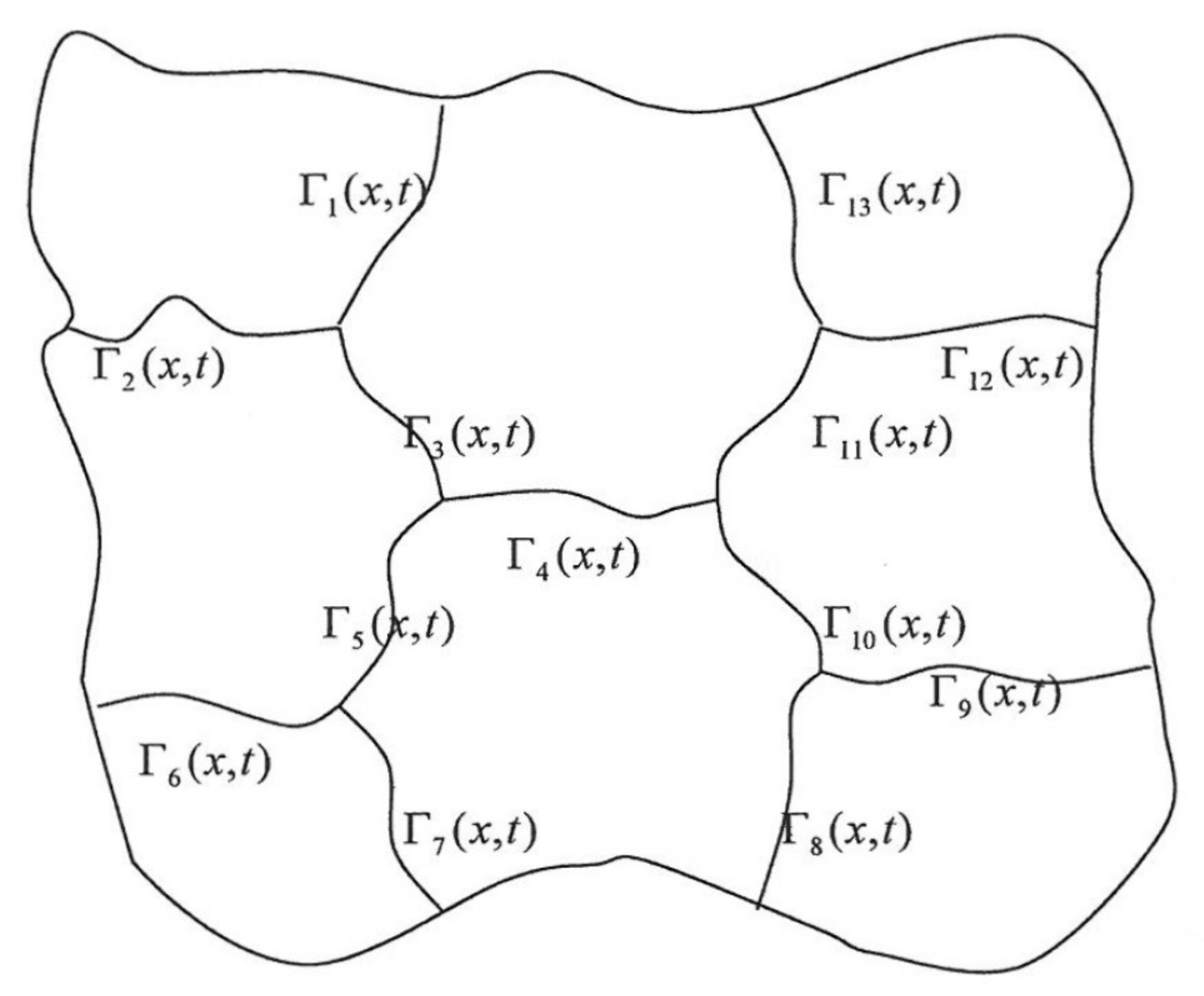
We will now consider a network with a minimum number of inner junctions. Let be a bounded domain with boundary and a network formed of triple junctions and , curves inside of , as seen in Figure 3. Based on (2), where is the solution of the following initial and boundary value problem:
with conditions of the following form:
- Incidence at the junctions:
- Incidence at the boundary :
- Angle conditions at the junctions:
- Angle conditions at :
Note that under these conditions, we have some sort of symmetry for the dynamical network under study. The eigenvalue problem (3) will then take the form:
with conditions:
- Incidence at the junctions:
- Incidence at the boundary :
- Angle conditions at the junctions:
- Angle conditions at :
The eigenvalues of (4) will give information about the stability of the network. Actually, we will prove that the stability depends on the geometry of the boundary .
Definition 2.
We define the sign of a curvature as follows. At the points at which a curve is convex, we define the sign of the curvature as positive, and at the points at which a curve is non-degenerate concave, we define the sign of the curvature as negative.
Theorem 1.
Let Ω be a bounded domain on the plane that contains a network formed by curves and triple junctions, including inner junctions, as seen in Figure 3. Then:
- (a)
- If the domain Ω is convex (an ellipse for example) at the points at which the steady state of the network meets the boundary, then the steady state is unstable.
- (b)
- If the domain Ω is non-degenerate concave at the points at which the steady state of the network meets the boundary, then the steady state is stable.
- (c)
- If the domain Ω is flat at the points at which the steady state of the network meets the boundary, then the steady state is neutrally stable.
Proof.
Since we study the stability of the steady states, we shall rewrite the eigenvalue problem (4) and its conditions by substituting , . Also note that by using Lemma 1, we can focus only on the functions . We have:
with conditions of the following form:
If , then the solution of (5) is equal to:
where , are unknown real variables. By replacing (6) into the conditions of (5), we get:
From the above equations, we have a homogeneous linear system of 26 unknowns (the real variables , , ) and 26 equations. In fact, by setting:
we can rewrite the above homogeneous linear system of equations in matrix form, i.e., , and get that the determinant of the matrix A is zero if and only if:
For the proof of (a), since is a strictly convex domain, we have , Hence, there exist given by (7), i.e., the determinant of the matrix A is zero, which means X is non-zero and consequently , ∀. Thus, the eigenvalue problem has negative eigenvalues, which are the solutions of (7), i.e., the eigenvalue problem (5) has negative eigenvalues, and the steady state is unstable.
For the proof of (b), since the curvature of the boundary (at the points at which it meets the network) is assumed negative, , , for , we have , , and hence, there do not exist such that (7) holds. Consequently, the determinant of the matrix A in non-zero and , i.e., , . Thus, the eigenvalue value problem (5) does not have negative eigenvalues, i.e., for , we get , . However, we need to consider the case of . By replacing this into (5), we get:
or, equivalently,
Furthermore, the conditions of (5) take the form:
The above homogeneous linear system has only the zero solution, i.e.,
Thus, for , we have , , i.e., the eigenvalue problem (5) does not have zero eigenvalues.
For the proof of (c), we have that the boundary is flat at the points where it meets the network (see Figure 4). This means that , In this case, since , (7) does not hold. Hence, the determinant of the matrix A in non-zero and , i.e., , . Thus, the eigenvalue value problem (5) does not have negative eigenvalues. In the case of , the differential Equation (5) takes the form:
or, equivalently,
Furthermore, the conditions take the form:
From the above equations, we get the solutions:
where are parameters. Hence, the problem has the zero eigenvalue. The zero eigenvalue has geometric multiplicity seven. The proof is completed. ☐
3. Hexagonal Network with an Internal Hexagon
In this section, we will study the case of a network of hexagons, with one of them having all its branches unattached to the boundary.
Definition 3.
A hexagonal network, which is part of a network inside a bounded domain, will be called an internal hexagon if all its curves have their ends unattached to the boundary.
We will now consider a network with one internal hexagon, i.e., a hexagonal network with the minimum number of hexagons that supports internal hexagons. We assume a bounded domain on the plane that contains a network formed by seven hexagons, one of which is internal. An example of the steady state of such a network is shown in Figure 5. As seen, the network has 24 junctions, 42 curves and 7 hexagons; 12 curves out of the 42 have one end attached to the boundary. Below we provide information regarding which curves are passing through each junction.
Junction 1 consists of Curves 1, 2, 3
Junction 2 consists of Curves 3, 4, 5
Junction 3 consists of Curves 5, 6, 7
Junction 4 consists of Curves 7, 8, 9
Junction 5 consists of Curves 9, 10, 11
Junction 6 consists of Curves 11, 12, 13
Junction 7 consists of Curves 13, 14, 15
Junction 8 consists of Curves 15, 16, 17
Junction 9 consists of Curves 17, 18, 19
Junction 10 consists of Curves 19, 20, 21
Junction 11 consists of Curves 21, 22, 23
Junction 12 consists of Curves 23, 24, 25
Junction 13 consists of Curves 25, 26, 27
Junction 14 consists of Curves 27, 28, 29
Junction 15 consists of Curves 29, 30, 31
Junction 16 consists of Curves 31, 32, 33
Junction 17 consists of Curves 33, 34, 35
Junction 18 consists of Curves 35, 1, 36
Junction 19 consists of Curves 36, 37, 38
Junction 20 consists of Curves 38, 6, 39
Junction 21 consists of Curves 39, 12, 40
Junction 22 consists of Curves 40, 18, 41
Junction 23 consists of Curves 41, 24, 42
Junction 24 consists of Curves 42, 30, 37.
Written in bold are the curves that have one end attached to the boundary. Based on (2), , is the solution of the following initial and boundary value problem:
with conditions:
- Incidence at the junctions:
- Incidence at the boundary :
- Angle conditions at the junctions:
- Angle conditions at :
Note that under these conditions, we have some sort of symmetry for the dynamical network under study. Furthermore, the eigenvalue problem (3) will take the form:
with conditions:
- Incidence at the junctions:
- Incidence at the boundary :
- Angle conditions at the junctions:
- Angle conditions at :
The eigenvalues of (8) will give information about the stability of the network. Actually, we will prove that stability depends on the geometry of the boundary .
Theorem 2.
Let Ω be a bounded domain on the plane that contains a hexagonal network with one internal hexagon; see Figure 5. Then:
- 1.
- If the domain Ω is convex (an ellipse for example) at the points where the steady state of the network meets the boundary, then the steady state is unstable.
- 2.
- If the domain Ω is non-degenerate concave at the points where the steady state of the network meets the boundary, then the steady state is stable.
- 3.
- If the domain Ω is flat at the points where the steady state of the network meets the boundary, then the steady state is neutrally stable.
Proof.
Since we study the stability of the steady states, we shall rewrite the eigenvalue problem (8) and its conditions substituting , . Note that by using Lemma 1, we can limit our study only to the function . We have:
with conditions of the following form:
Under these conditions, we have some sort of symmetry at the steady states for the network under study. For more details about the structure, the symmetry and the hexagon decomposition that appears, see [11]. If , then the solution of (9) is equal to:
where , are unknown real variables. By replacing (10) into the conditions, we have:
We have a homogeneous linear system of 84 unknowns (the real variables , , ) and 84 equations. In fact, by rewriting the above homogeneous linear system of equations in a matrix form , where and by using MATLAB, we get that the determinant of the matrix is zero if and only if:
For the proof of (a), since is a strictly convex domain, . Hence, there exist given by (11), i.e., the determinant of A is zero and X has infinitely many solutions. Thus, the eigenvalue problem (9) has negative eigenvalues, and the steady state is unstable.
For the proof of (b), the curvature of the boundary is negative at the points where it meets the network (). This means that (11) does not hold and the determinant of the matrix A is non-zero. Hence , i.e.,
or, equivalently,
Thus, the problem does not have negative eigenvalues. In the case of , (9) takes the form:
or, equivalently,
Furthermore, the conditions take the form:
Note that because of the symmetry that appears in several parts at the steady states, every solution of a difference equation related to the ’ s is periodic with a period of three. From the above equations, , Then, the remaining unknowns will be 42 with 36 linear independent equations. This means that we will have eigenfunctions independent of x, and their eigenspace will have dimension six. Since the network contains six hexagons attached to the boundary (seven in total), from the von Neumann–Mullins theorem, the network does not destabilise, but only rotates.
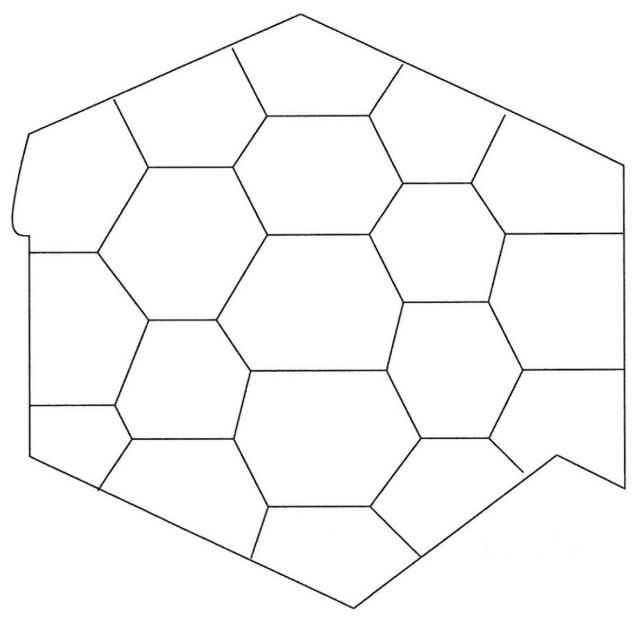
For the proof of (c), we have that the boundary is flat at the points where it meets the network. This means that ; see Figure 6.
In this case, since , (11) does not hold. Hence, the determinant of the matrix A in non-zero and , i.e., , Thus, the eigenvalue value problem (9) does not have negative eigenvalues. In the case of , the differential Equation (9) takes the form:
or, equivalently,
Furthermore, the conditions take the form:
From the above equations , . Then, the remaining unknowns will be 42 with 24 linear independent equations. This means that we will have eigenfunctions independent of x and their eigenspace will have dimension 18. The zero eigenvalue has geometric multiplicity 18. The proof is completed.
4. Conclusions
In this article, we studied two problems of dynamical networks in the planar domain formed by triple junctions, with some symmetry, fixed angle conditions at the points at which they intersect and the normal velocity proportional to the curvature. We introduced the geometric evolution problem and studied the stability of two cases, a network where two triple junctions have all their branches unattached to the boundary and a network of hexagons, with one of them having all its branches unattached to the boundary. In both cases, conditions were identified under which the steady states of these networks are stable, unstable and neutrally stable. A further extension of this article is the stability investigation of mixed domains (i.e., the case where at least two types of domains appear during the evolution) and 3D evolution problems. Finally, there are very interesting applications that could be studied further such as:
- Grain growth problems: the increase in the size of grains (crystallites) in a material at high temperatures;
- Neural networks that can be applied on the decomposition system (3) for ;
- Continuum modelling of electromechanical dynamics in large-scale power systems;
- Electrical networks of power systems that are not static and change their shape in time. This type of network can include synchronization problems of nonlinear circuits in dynamic electrical networks with general topologies and power system cascading risk assessment based on complex network theory.
For all these issues, there is already some research in progress.
Acknowledgments
I. Dassios is funded by the Science Foundation Ireland (Strategic Partnership Programme Grant Number SFI/15/SPP/E3125).
Conflicts of Interest
The author declares no conflicts of interest.
References and Note
- Bellettini, G.; Chermisi, M.; Novaga, M. Crystalline curvature flow of planar networks. Interfaces Free Bound. 2006, 8, 481–521. [Google Scholar] [CrossRef]
- Fried, E.; Gurtin, M.E. Gradient nano-scale polycrystalline elasticity: inter grain interactions and triple-junction conditions. J. Mech. Phys. Solids 2009, 57, 1749–1779. [Google Scholar] [CrossRef]
- Gurtin, M.E.; Anand, L. Nano-crystalline grain boundaries that slip and separate: A gradient theory that accounts for grain-boundary stress and conditions at a triple-junction. J. Mech. Phys. Solids 2008, 56, 184–199. [Google Scholar] [CrossRef]
- Corematerials. Growth of a Two-Dimensional Grain Structure. 2009. Available online: https://www.youtube.com/watch?v=J_2FdkRqmCA (accessed on 1 December 2017).
- Graham, H. An Introduction to Hexagonal Geometry. 2010. [Google Scholar]
- Pappas, T. Hexagons in Nature. In The Joy of Mathematics; Wide World Publ./Tetra: San Carlos, CA, USA, 1989; pp. 74–75. [Google Scholar]
- Alama, S.; Bronsard, L.; Gui, C. Stationary layered solutions in R2 for an Allen-Cahn system with multiple well potential. Calc. Var. Partial Differ. Equ. 1997, 5, 359–390. [Google Scholar] [CrossRef]
- Bronsard, L.; Gui, C.; Schatzman, M. A three-layered minimizer in R2 for a variational problem with a symmetric three-well potential. Commun. Pure. Appl. Math. 1996, 49, 677–715. [Google Scholar] [CrossRef]
- Bronsard, L.; Whetton, B. Numerical method for tracking curve networks moving with curvature motion. J. Comput. Phys. 1995, 120, 66–87. [Google Scholar] [CrossRef]
- Bronsard, L.; Reitich, F. On three-phase boundary motion and the singular limit of a vector-valued Ginzburg-Landau equation. Arch. Ration. Mech. 1993, 124, 355–379. [Google Scholar] [CrossRef]
- Freire, A. Mean Curvature Motion of Triple Junctions of Graphs in Two Dimensions. Commun. Partial Differ. Equ. 2010, 35, 302–327. [Google Scholar] [CrossRef]
- Ikota, R.; Yanagida, E. Stability of stationary interfaces of binary-tree type. Calc. Var. Partial Differ. Equ. 2004, 22, 375–389. [Google Scholar] [CrossRef]
- Tortorelli, C.; Mantegazza, M.; Novaga, V.M. Motion by Curvature of Planar Networks. arXiv, 2003; arXiv:math/0302164v1. [Google Scholar]
- Xiaofeng, R.; Wei, J. A Double Bubble in a Ternary System with Inhibitory Long Range Interaction. Arch. Ration. Mech. Anal. 2013, 208, 201–253. [Google Scholar]
- Baake, M.; Ghler, F.; Grimm, U. Hexagonal inflation tilings and planar monotiles. Symmetry 2012, 4, 581–602. [Google Scholar] [CrossRef]
- Dassios, I.; Jivkov, A.; Abu-Muharib, A.; James, P. A mathematical model for plasticity and damage: A discrete calculus formulation. J. Comput. Appl. Math. 2017, 312, 27–38. [Google Scholar] [CrossRef]
- Esqueda, H.; Herrera, R.; Botello, S.; Moreles, M.A. A geometric description of Discrete Exterior Calculus for general triangulations. arXiv, 2018; arXiv:1802.01158. [Google Scholar]
- Esqueda, H.; Herrera, R.; Botello, S.; Moreles, M.A. Discrete Exterior Calculus for General Triangulations; ResearchGate: Rome, Italy, 2018. [Google Scholar]
- Garlaschelli, D.; Ruzzenenti, F.; Basosi, R. Complex Networks and Symmetry I: A Review. Symmetry 2010, 2, 1683–1709. [Google Scholar] [CrossRef]
- Hou, L.; Small, M.; Lao, S. Dynamical Systems Induced on Networks Constructed from Time Series. Entropy 2015, 17, 6433–6446. [Google Scholar] [CrossRef]
- Nguyen, T.-T.; Le, D.V.; Yoon, S. Maximization of the Supportable Number of Sensors in QoS-Aware Cluster-Based Underwater Acoustic Sensor Networks. Sensors 2014, 14, 4689–4711. [Google Scholar] [CrossRef] [PubMed]
- Ruzzenenti, F.; Garlaschelli, D.; Basosi, R. Complex Networks and Symmetry II: Reciprocity and Evolution of World Trade. Symmetry 2010, 2, 1710–1744. [Google Scholar] [CrossRef]
- Wang, X.; Jiang, G.-P.; Wu, X. State Estimation for General Complex Dynamical Networks with Incompletely Measured Information. Entropy 2018, 20, 5. [Google Scholar] [CrossRef]
- Boutarfa, B.; Dassios, I. A stability result for a network of two triple junctions on the plane. Math. Methods Appl. Sci. 2015, 40, 6076–6084. [Google Scholar] [CrossRef]
- Dassios, I. Stability of basic steady states of networks in bounded domains. Comput. Math. Appl. 2015, 70, 2177–2196. [Google Scholar] [CrossRef]
- Dassios, I. Stability of triple junctions on the plane. Bull. Greek Math. Soc. 2007, 54, 281–300. [Google Scholar]
- Yanagida, E.; Ikota, R. A stability criterion for stationary curves to the curvature driven-motion with a triple junction. Differ. Integral Equ. 2003, 16, 707–726. [Google Scholar]
Figure 1.
Evolution of a network in 57 s.

Figure 2.
Polycrystalline camphor-ethanol mixture, soap bubbles and honeycomb.
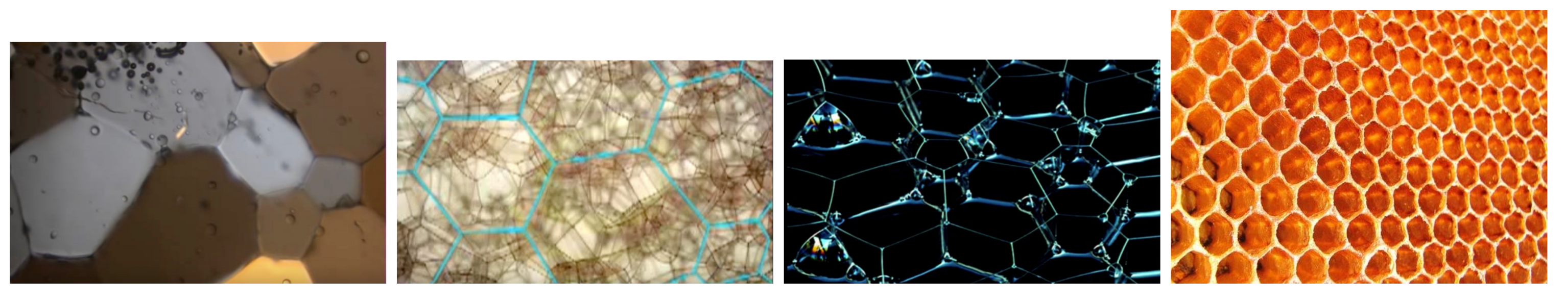
Figure 3.
A bounded network with two inner triple junctions.

Figure 4.
Flat boundary at the points where it meets the network.
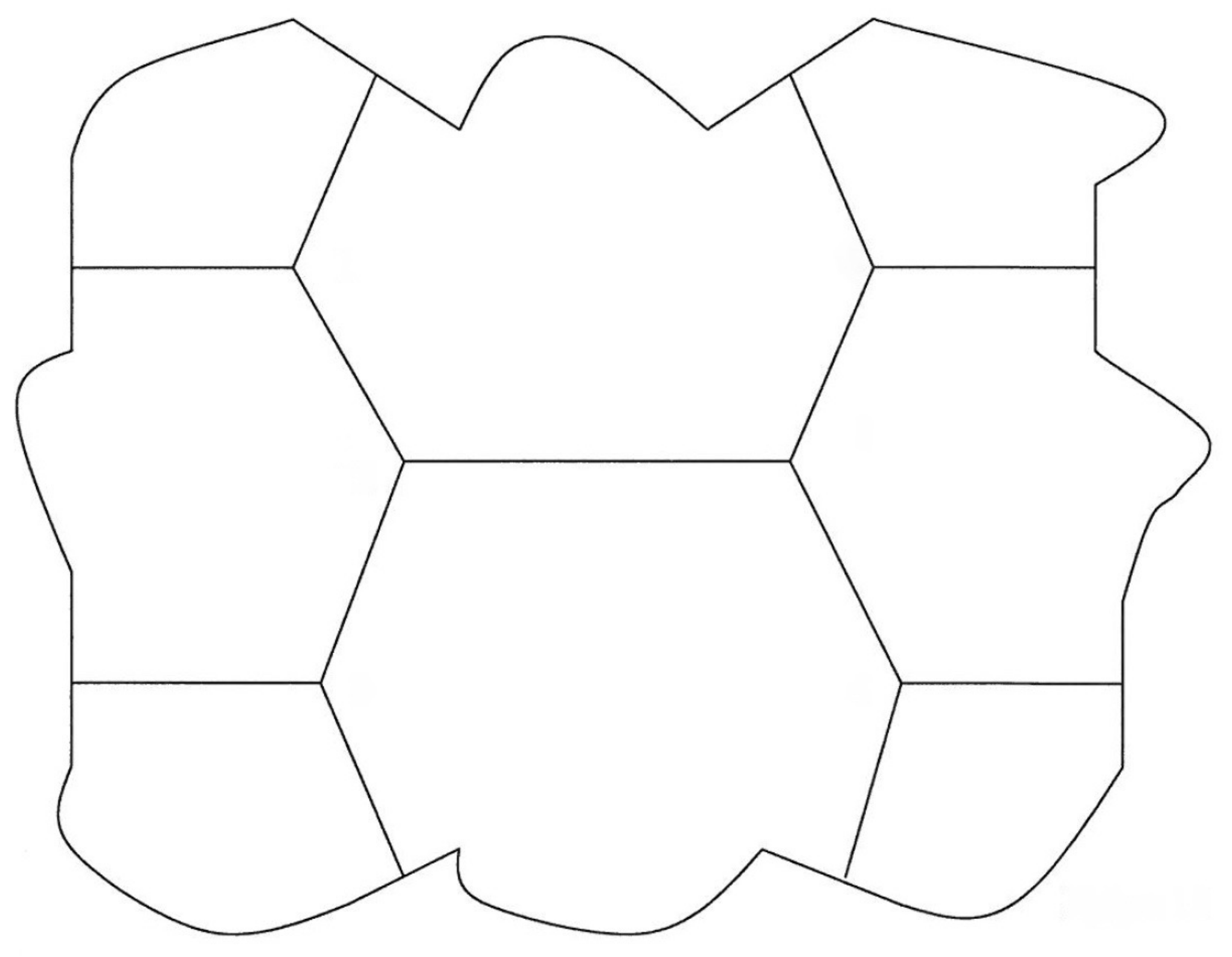
Figure 5.
Hexagonal network with an internal hexagon.
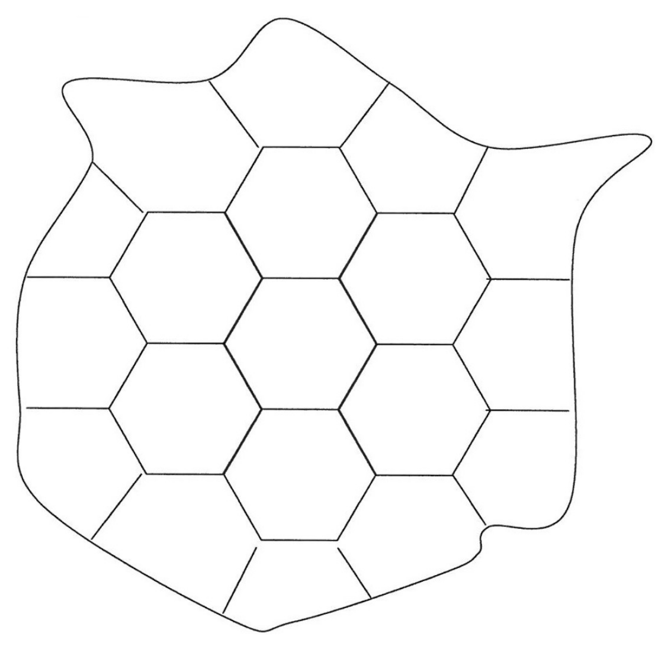
Figure 6.
Flat boundary at the points where it meets the network.
© 2018 by the author. Licensee MDPI, Basel, Switzerland. This article is an open access article distributed under the terms and conditions of the Creative Commons Attribution (CC BY) license (http://creativecommons.org/licenses/by/4.0/).
Share and Cite
MDPI and ACS Style
Dassios, I.K. Stability of Bounded Dynamical Networks with Symmetry. Symmetry 2018, 10, 121. https://doi.org/10.3390/sym10040121
AMA Style
Dassios IK. Stability of Bounded Dynamical Networks with Symmetry. Symmetry. 2018; 10(4):121. https://doi.org/10.3390/sym10040121
Chicago/Turabian StyleDassios, Ioannis K. 2018. "Stability of Bounded Dynamical Networks with Symmetry" Symmetry 10, no. 4: 121. https://doi.org/10.3390/sym10040121
Note that from the first issue of 2016, this journal uses article numbers instead of page numbers. See further details here.