Multimedia System for Real-Time Photorealistic Nonground Modeling of 3D Dynamic Environment for Remote Control System


1
Department of Multimedia Engineering, Dongguk University-Seoul, 30, Pildongro-1-gil, Jung-gu, Seoul 04620, Korea
2
2nd R&D Institute, Agency for Defense Development, P.O. Box 35, Yuseong-gu, Daejeon 34186, Korea
*
Author to whom correspondence should be addressed.
Symmetry 2018, 10(4), 83; https://doi.org/10.3390/sym10040083
Submission received: 31 January 2018
/
Revised: 8 March 2018
/
Accepted: 26 March 2018
/
Published: 28 March 2018
(This article belongs to the Special Issue Advanced in Artificial Intelligence and Cloud Computing)
Abstract
:Nowadays, unmanned ground vehicles (UGVs) are widely used for many applications. UGVs have sensors including multi-channel laser sensors, two-dimensional (2D) cameras, Global Positioning System receivers, and inertial measurement units (GPS–IMU). Multi-channel laser sensors and 2D cameras are installed to collect information regarding the environment surrounding the vehicle. Moreover, the GPS–IMU system is used to determine the position, acceleration, and velocity of the vehicle. This paper proposes a fast and effective method for modeling nonground scenes using multiple types of sensor data captured through a remote-controlled robot. The multi-channel laser sensor returns a point cloud in each frame. We separated the point clouds into ground and nonground areas before modeling the three-dimensional (3D) scenes. The ground part was used to create a dynamic triangular mesh based on the height map and vehicle position. The modeling of nonground parts in dynamic environments including moving objects is more challenging than modeling of ground parts. In the first step, we applied our object segmentation algorithm to divide nonground points into separate objects. Next, an object tracking algorithm was implemented to detect dynamic objects. Subsequently, nonground objects other than large dynamic ones, such as cars, were separated into two groups: surface objects and non-surface objects. We employed colored particles to model the non-surface objects. To model the surface and large dynamic objects, we used two dynamic projection panels to generate 3D meshes. In addition, we applied two processes to optimize the modeling result. First, we removed any trace of the moving objects, and collected the points on the dynamic objects in previous frames. Next, these points were merged with the nonground points in the current frame. We also applied slide window and near point projection techniques to fill the holes in the meshes. Finally, we applied texture mapping using 2D images captured using three cameras installed in the front of the robot. The results of the experiments prove that our nonground modeling method can be used to model photorealistic and real-time 3D scenes around a remote-controlled robot.
1. Introduction
In recent years, many multimedia applications using multi-sensors have been proposed. These applications are widely used in many areas, such as artificial intelligence in cloud environments [1,2], Internet of Things (IoT) [3], virtual reality [4], and unmanned ground vehicles (UGVs) [5,6,7,8,9,10,11,12]. This study is related to multi-sensor data processing for UGV control. UGVs are often employed in areas where the terrain is rough, dangerous, or impossible to navigate for a human operator. UGVs are of two main types: autonomous and remote controlled. In both cases, sensors are installed to collect information regarding the environment surrounding the vehicle. In particular, for a remote-controlled robot [9,10,11,12], we usually employ multi-channel laser sensors, two-dimensional (2D) cameras, and Global Positioning System–inertial measurement unit (GPS–IMU) sensors. Each laser range sensor returns a point cloud frame-by-frame. Based on the 2D images obtained from the cameras and the position and direction obtained from the GPS–IMU sensors, we can reconstruct the three-dimensional (3D) scene of the working environment of a robot from the point clouds. 3D scene modeling is highly important for any remote-controlled robot system. From the reconstructed 3D scene surrounding the robot, a user can remotely control the robot in a more accurate manner. Therefore, the modeling of a 3D scene from point clouds has been gaining considerable interest, with various studies having already been conducted [9,10,11,12,13,14,15,16]. However, establishing an efficient trade-off between real-time and high-quality modeling is a challenging problem, for which a solution is actively being pursued.
Before modeling an outdoor terrain, we often divide a point cloud into two areas: ground and nonground. In general, modeling the ground part is simpler than modeling the nonground part. The modeling of the nonground part is more difficult in dynamic environments with many moving objects than in static environments because of two reasons: (1) we may lose many points on the moving objects in each frame, resulting in holes when the data are reconstructed; and (2) the trace data of the moving objects develop into long chains when many frames are collected.
Hence, in this study, we focused on modeling the nonground part of the terrain in a dynamic environment. Our objective was to design a fast and photorealistic modeling method. For a better reconstruction quality, we used images captured using 2D cameras attached to the front of the robot to implement texture mapping and obtain colored particles. In addition, we applied an existing method [9] to model the ground part using the robot location and height map. The ground modeling was implemented using a graphics processing unit (GPU) for speed-up. After modeling both parts, we combined the results for visualization.
The remainder of this paper is organized as follows. In Section 2, we provide an overview of the studies related to surface reconstruction and 3D scene modeling. Section 3 presents our novel method. In Section 4, the experiments and analyses are discussed. Finally, we summarize the main conclusions of this study and present the direction of our future work in Section 5.
2. Related Works
Many studies conducted in the past few years have focused on 3D scene modeling for remote-controlled robots [9,10,11,12]. However, the performance of these modeling methods is poor. We broadly categorize these techniques and algorithms in relation to our present research as follows.
In [10,11], the authors employed colored particles to model nonground objects. This method is fast and has an adaptive real-time performance. The particle modeling results are photorealistic in the far view, but quite poor in the near view. Although this method is suitable for non-surface objects, such as trees or bushes, the reconstruction quality of surface objects, such as walls or buildings, is not photorealistic. Kelly at al. [12] presented a modeling method for reconstructing walls. The authors used small cubes stacked on top of each other like Legos. However, a good photorealistic result cannot be obtained using the cube method because of the low display resolution.
In addition, the authors [13,14,15,16] proposed different methods for reconstructing 3D point clouds using the Delaunay triangulation algorithm. These methods exhibited high surface quality; however, they are time-consuming. Some authors have proposed parallel algorithms using a GPU [15,16]; however, the performance does not meet the real-time requirement. Therefore, these methods are only suitable for modeling small objects with dense point clouds. Because of this limitation, these methods are inefficient for remote-controlled robots in both indoor and outdoor environments.
The above limitations motivated us to develop an approach that can achieve a higher modeling quality and real-time performance in dynamic outdoor environments. In our method, a fast object segmentation and tracking algorithm was required. In previous studies [17,18,19,20,21,22,23,24,25,26,27,28,29,30,31,32,33,34,35], the authors proposed numerous detection and tracking-of-moving-objects (DATMO) systems. However, DATMO systems are time-consuming because of the high computation complexity. Therefore, in this study, we employed our previous DATMO system [36,37,38] to detect dynamic objects and collect points on the dynamic objects in previous frames. In addition, because of the dynamic environment, an algorithm is required to eliminate the traces of dynamic objects. To this end, we employed our previous study [39] for trace elimination. For texture mapping and color projection between 2D images and 3D points, we employed the extrinsic calibration algorithm proposed elsewhere [40]. As mentioned previously, to model the ground part, we employed an existing method [9] based on the height map and robot location.
3. Proposed Method
The main objective of our study was to design a fast 3D modeling method for nonground parts in a dynamic environment. Figure 1 shows the proposed system framework. The proposed system is inputted with 3D nonground points. As mentioned above, the nonground points are obtained after applying the segmentation algorithm. In the first step, the nonground points are segmented into separate objects based on a flood-fill algorithm proposed elsewhere [37]. In the second step, a fast object tracking algorithm [38] is applied to obtain a list of dynamic objects. Based on the length and width of each object, we easily separated large and small dynamic objects. The large and small objects are described in more detail in Section 3.2 and Section 4. In the third step, based on the lists of objects and dynamic objects in the current frame, we propose a surface object detection algorithm, which is presented in Section 3.1. After the third step, the objects were divided into three groups: large dynamic objects, surface objects, and non-surface objects. The small dynamic objects are considered in the non-surface group. We collected all the points on these objects for modeling using a different method. Before the modeling, we used a trace elimination method proposed elsewhere [39] to remove past data of the moving objects. For the non-surface objects, we employed the colored particle method [9]. On the other hand, we propose a new mesh modeling method based on two dynamic projection panels for surface and large dynamic objects. The mesh modeling method is proposed in Section 3.2. After the mesh generation step, we employed slide window and near point projection techniques for mesh enhancement, as shown in Section 3.3. Next, we designed a texture mapping method, which is given in Section 3.4. The mesh modeling results are used for both visualization and maintainable checking. The maintainable checking step is implemented to save the modeling results of the static surface objects for subsequent visualization. We describe the maintainable checking step in Section 3.5. Finally, the colored particles, current mesh modeling results, and accumulated results are combined for visualization.
3.1. Surface Object Detection
In this section, we present a detection algorithm for surface objects, which are objects having a roughly flat shape, such as walls and buildings. In addition, objects having a curved surface, such as cars and lighthouses, are considered surface objects. Non-surface objects include bushes and trees. Small and tall-thin objects, such as pedestrians, lamps, and traffic lights, are also considered non-surface objects. First, we divide each object into vertical lines. We assume an m-channel laser scanner. Each vertical line connects all the points from scanline 0 to scanline m − 1 at the scanning time. We ignore all the lost points on the vertical lines because they have no location information. The vertical lines are indicated in red, as shown in Figure 2.
Using Equation (1), we calculated the distortion value di corresponding to all the vertical lines in the three objects. These objects were chosen because they are the most representative of the surface and non-surface objects in the outdoor environment. Here, (, ) is the location of point Pj in the Oxz coordinate, and n is the number of points on the vertical line i. Ex,i and Ez,i are the mean values of line i along the Ox and Oz directions, respectively.
Figure 3 shows the distortion values of a tree, car, and wall. The red line represents the distortion values of the tree, which are significantly higher than those of the car and wall. Based on this observation, we separated the surface and non-surface objects. The details of the method are shown in Algorithm 1. We applied the CHECK_SURFACE_OBJECT() function for all the objects. The return values 0, 1, and 2 correspond to non-surface, surface, and large dynamic objects, respectively.
| Algorithm 1. Surface object detection. |
| Function CHECK_SURFACE_OBJECT(Object obj) |
| h←obj. Get_Height() |
| w←obj. Get_Width() |
| If obj. Get_Object_Type() = Dynamic then |
| If h < dSmall AND w < dSmall then |
| Return 0 //non-surface object |
| Else |
| Return 2 //large dynamic object |
| End |
| Else if h < dSmall AND w < dSmall then |
| Return 0 //non-surface object |
| End |
| ns←0 |
| For i = 0. n − 1 do |
| d←obj. Calculate_Distortion() |
| If d < dmax then |
| ns←ns + 1 |
| End |
| End |
| r←ns/n |
| If r > rmin then |
| Return 1 //surface object |
| Else |
| Return 0 //non-surface object |
| End |
3.2. 3D Mesh Generation for Nonground Surfaces
In the mesh generation step, we generated triangular meshes for all the surface objects. The large dynamic objects, such as cars and trucks, were also modeled using meshes, whereas small dynamic objects, such as pedestrians and cyclists, were modeled using particles. Figure 4 shows the overview of the mesh generation method. In our system, we installed three 2D cameras in the front of the robot; therefore, the back area has no information for texture mapping. A camera was set up facing the front direction of the robot. Two more cameras were installed on the left and right of the first camera at 45°. Because of this limitation, only the area in front of the robot could be reconstructed.
In each frame, two dynamic projection panels were created at infinity. The angle between each panel and the direction of the robot is 45°. We divided the points on the surfaces and large dynamic objects into two parts. The points located in area 1 (left) are projected onto the left panel. The remaining points are projected onto the right panel. Once a point is projected onto a panel, the depth value of the corresponding quantized points in the panel will be updated. After projecting all the points on the surface and large dynamic objects, we generated triangular meshes from each panel. The generation method is similar to the generation of ground meshes. We saved the generated meshes using the mesh node model. Each mesh node contains a vertex node, an index node, and a texture node. Details regarding this are given in Section 3.4.
3.3. Mesh Enhancement
In the mesh enhancement step, we applied two techniques to enhance the quality of the meshes. First, we used a sliding window for filling the holes in each mesh panel. Figure 5 shows a 7 × 7 slide window used for filling holes. The sliding window is indicated in yellow, whereas the scanning area is indicated in green. If the center position of the window has no mesh point, we consider the center horizontal row and the center vertical column of the sliding window. If there are at least two points located on the “left and right” or “up and down” of the center position, we insert the new point at the center with the average coordinate values of the existing points in the sliding window.
In addition, we proposed another technique to enhance the mesh quality. We consider all the particles near any surface objects. If the distance between a particle and a mesh point is small, the particle is removed. Figure 6 shows an example of this technique. Particles 1 to 4 are removed because they are located near the mesh points. Moreover, particles 5 to 7 are removed; however, they help in adding two new mesh points.
3.4. Texture Mapping
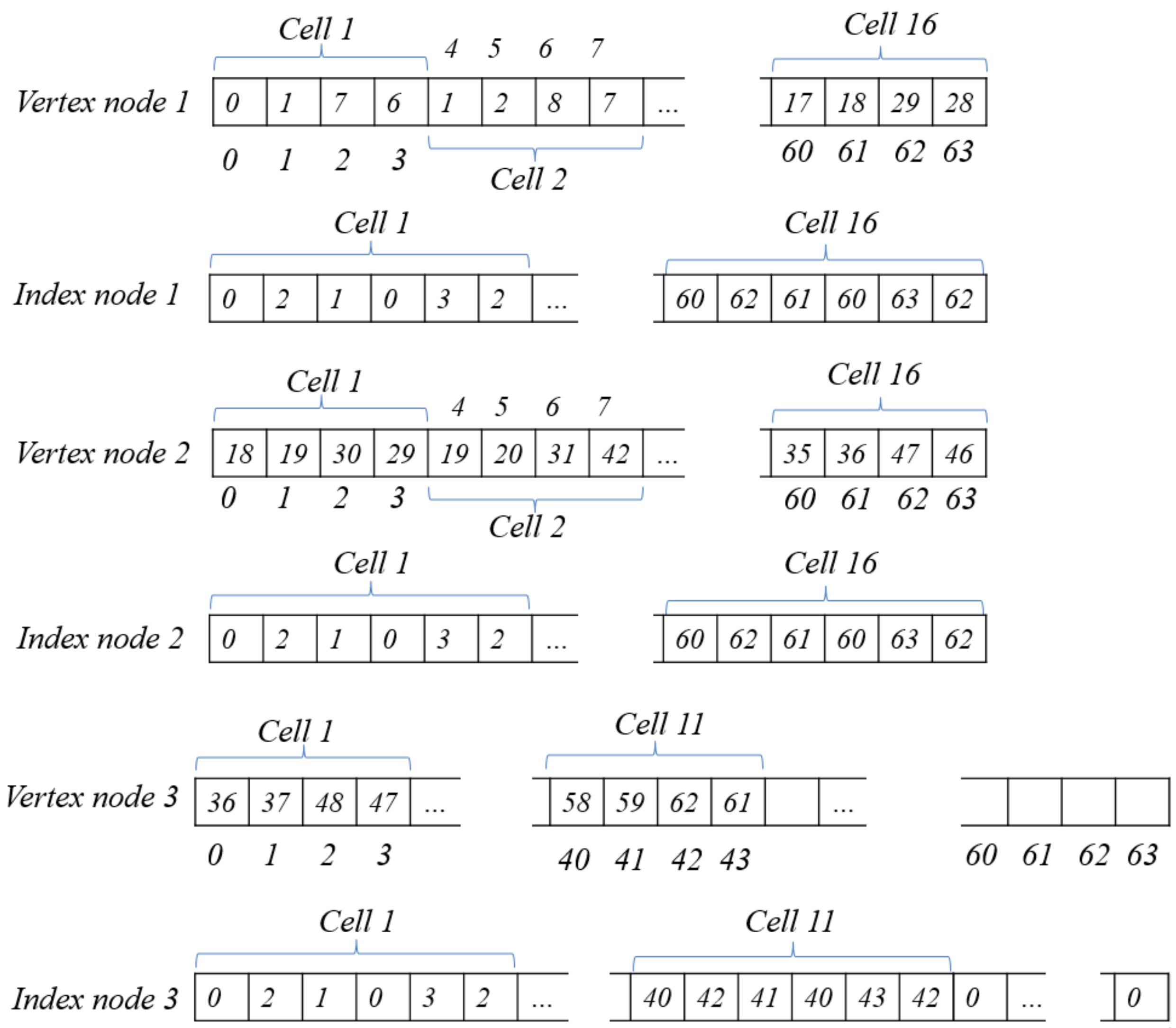
In this section, we propose an optimization texture mapping method for surface objects. As mentioned above, the generated meshes are saved using the mesh node model, as shown in Figure 7 and Figure 8. For saving the textures, we created several texture nodes corresponding to the vertex and index nodes. We used a square texture node. Each texture node contains k × k cells. Each texture cell maps with four vertices in the vertex node and six indices in the index node. For each texture node, we calculated the UV mapping using Algorithm 2. If two projection panels with a size of (width × height) are used, we require texture nodes, which can be calculated using Equation (2). Figure 9 shows an example of the texture nodes with k = 4. Each texture node has 16 texture cells. The texture nodes 1, 2, and 3 are saved with the textures of green, red, and blue areas, shown in Figure 7, respectively. Texture nodes 1 and 2 are full. On the other hand, texture node 3 has five blank cells. The empty cells will be used for other meshes.
| Algorithm 2. Calculate UV for texture mapping. |
| Procedure CALCULATE_UV() |
| For i = 0..k×k do |
| row←i/k |
| col←i – row × k |
| u[i×4]← col/k |
| v[i×4]← (row + 1)/k |
| u[i×4 + 1]←(col + 1)/k |
| v[i×4 + 1]←(row + 1)/k |
| u[i×4 + 2]←(col + 1)/k |
| v[i×4 + 2]←row/k |
| u[i×4 + 3]←col/k |
| v[i×4 + 3]←row/k |
| End |
3.5. Maintenance of Mesh Modeling Results
In this step, we maintain a part of the previous mesh modeling results of the static surface objects such as walls and buildings. Large dynamic objects are not retained and are re-modeled in the next frame. If we maintain all modeling results of the surface objects in each frame, the data will overlap. This problem takes up considerable memory for saving the modeling results because the used memory in the next frame includes all the used memory from the initial frame to the current frame. In addition, this problem leads to a flickering visualization error. To solve these problems, we divided the space into three parts, as shown in Figure 4. In the reconstruction area, the previous mesh modeling results are deleted. Otherwise, the previous modeling results of the surface objects are maintained in the maintainable area. In the overlapping area, we saved only the center points of each cell. Thereafter, we combined the center points with the point clouds of the surface and large dynamic objects for subsequent modeling.
4. Experiments and Analysis
We conducted several experiments to verify the effectiveness of our nonground modeling method in dynamic environments. The data were obtained from a Velodyne HDL-32E sensor, a GPS–IMU sensor, and three 2D cameras attached to a moving robot. The datasets were captured in both static and dynamic environments. The environments included many moving objects, surface objects, and non-surface objects.
For the experiments, a computer with an Intel Core i7-6700 CPU (3.4 GHz) and 16 GB of RAM was used. In addition, we used an NVIDIA GTX-970 graphics card and 4 GB of VRAM. For the object segmentation and object tracking steps, we employed the parameters employed elsewhere [38]. In the trace elimination step, the size of each voxel was 40 × 40 × 40 cm3. We used two voxel maps, each with a size of 100 × 100 × 100 (width × height × depth). Currently, the system can be used to filter a 40 × 40 × 40 m3 space. For the mesh modeling step, we created two projection panels with a size of 100 × 100 (width × height). In addition, the size of each cell was 30 × 30 cm2 for initialization. We set α = 60° and β = 10°. For the other LiDAR sensors, different parameters were chosen based on the resolution of the laser sensors. For the surface object detection algorithm, we set dSmall = 1 m, dmax = 30 cm, and rmin = 0.5.
We employed a node texture with 128 × 128 cells. The resolution of each texture cell was 8 × 8 pixels. Hence, the resolution of each texture node was 1024 × 1024 pixels. Based on Equation (2), only two mesh nodes are required for each frame. The three 2D cameras returned three images per frame, with a resolution of 640 × 480 pixels. These images were used for the texture mapping step.
4.1. Experimental Results
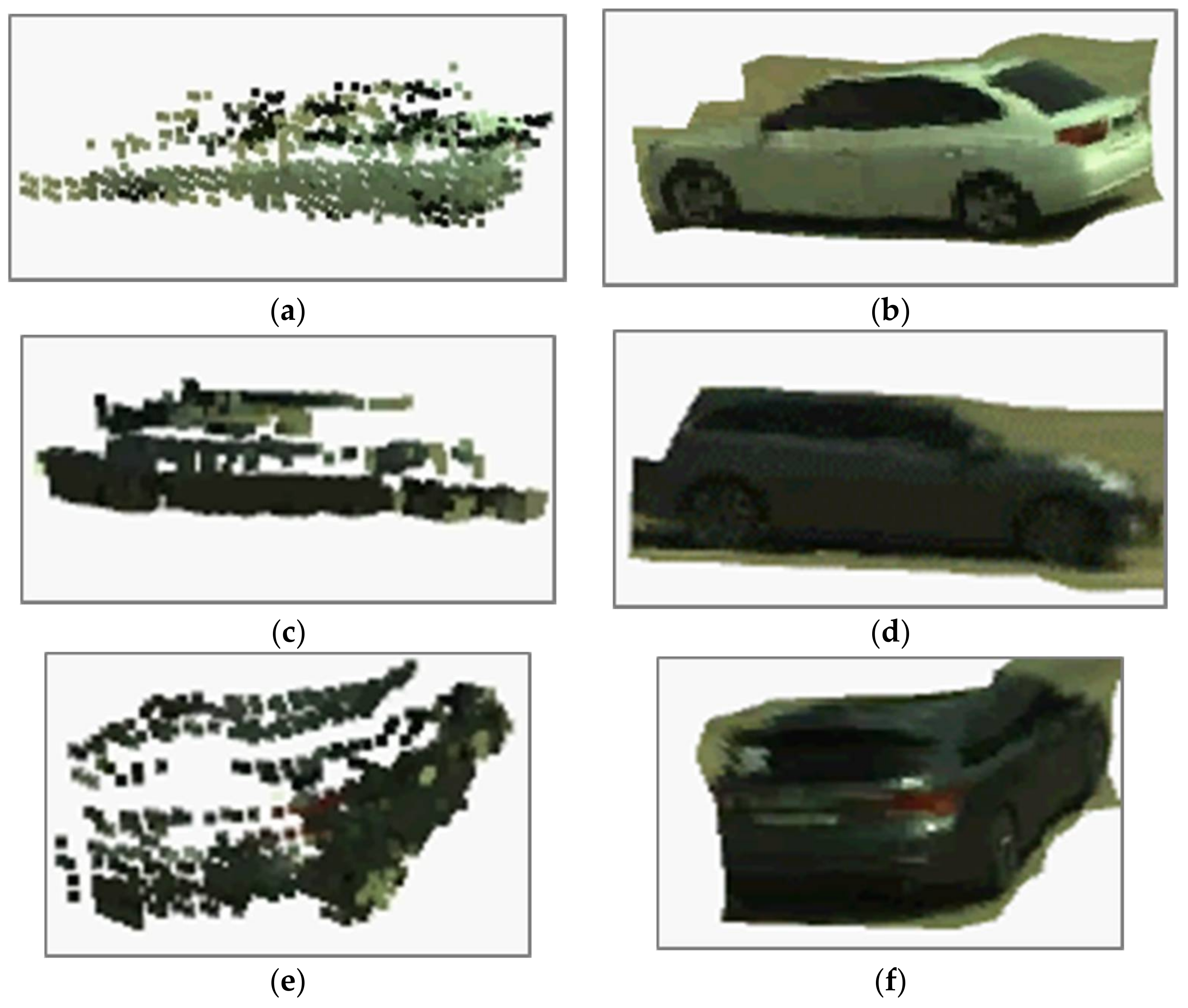
Figure 10 shows the results of the proposed method for large dynamic, surface, and non-surface objects. In Figure 10, the images on the left show the wire-frame mode, whereas the images on the right show the final results after the mapping texture. Figure 11 and Figure 12 show the results of the full system, including the ground and nonground modeling. Walls, buildings, and cars were efficiently modeled using the mesh method. Trees, bushes, and tall-thin objects were modeled using the colored particle method. All the experiments show photorealistic results in both the far and near views, thus proving the effectiveness of the proposed nonground modeling method.
4.2. Experimental Analysis
We compared our proposed mesh modeling method with the colored particle method [10,11,12]. Figure 13 shows the comparison results for the static surface objects such as walls and buildings. Figure 14 shows the comparison results for large moving objects such as cars. In both the cases, our method provides better photorealistic results than the previous methods. Because Velodyne HDL-32E has a low resolution in the vertical direction, the reconstruction results using particles contain many holes and blank areas. In our method, we applied some techniques to fill the holes, thereby significantly enhancing the quality.
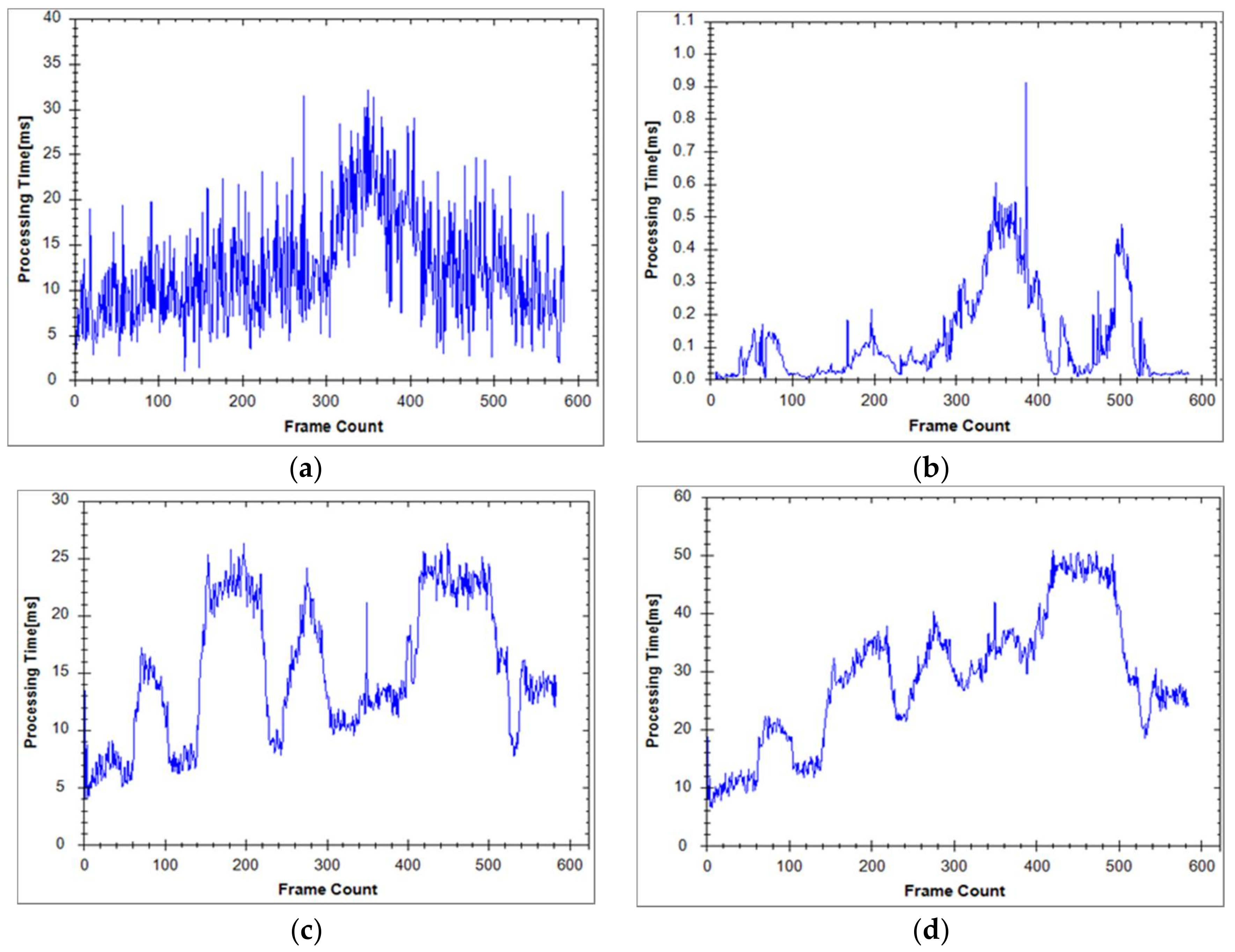
Furthermore, the processing time of each step was recorded, as shown in Figure 15 and Table 1. Figure 15d shows the total processing time with respect to the frame count for the proposed nonground modeling method. Table 1 lists the processing times of each step in the full modeling system. In each frame, we processed approximately 100,000 accumulated points for particle modeling and 100,000 accumulated points for mesh modeling. The average processing time of the proposed nonground modeling for each frame was 28.98 ms. The full system requires 93.61 ms per frame. Hence, we were able to process more than 10 frames per second (fps). In addition, the Velodyne HDL-32E sensor works at a rate of 10 fps. Thus, our 3D scene modeling system can perform effectively in real time.
5. Conclusions
In this paper, we focused on a fast and efficient method for modeling nonground objects using multiple types of sensor data. For nonsurface objects, we applied the colored particle method. On the other hand, we implemented the mesh modeling method based on two projection panels for surface and large dynamic objects. For ground modeling, we applied an existing method. To conduct the experiments, we employed a multi-channel LiDAR sensor, a GPS–IMU sensor, and three 2D cameras. The experimental results show that our method is able to achieve high reconstruction quality in real time. For the Velodyne HDL-32E sensor, the presented approach required only 28.98 ms for the nonground modeling per frame. Moreover, the full modeling system was able to perform in real time. However, the processing time required for the ground modeling was quite high. In the near future, we intend to upgrade our modeling system to further reduce the processing time required for ground modeling and enable it to operate in different types of complex terrains.
Acknowledgments
This research was supported by a grant from Agency for Defense Development, under contract #UD150017ID and by BK21 Plus project of the National Research Foundation of Korea Grant.
Author Contributions
Phuong Minh Chu and Seoungjae Cho wrote the source code. Sungdae Sim suggested that surface object detection was needed to improve the visualization performance of this technique. Kyungeun Cho and Kiho Kwak contributed to the discussion and analysis of the results. Phuong Minh Chu wrote the paper. All authors have read and approved the final manuscript.
Conflicts of Interest
The authors declare no conflict of interest.
References
- Lim, J.B.; Gil, J.M.; Yu, H.C. A Distributed Snapshot Protocol for Efficient Artificial Intelligence Computation in Cloud Computing Environments. Symmetry 2018, 10, 30. [Google Scholar] [CrossRef]
- Lim, J.B.; Yu, H.C.; Gil, J.M. An Efficient and Energy-Aware Cloud Consolidation Algorithm for Multimedia Big Data Applications. Symmetry 2017, 9, 184. [Google Scholar] [CrossRef]
- Maity, S.; Park, J.H. Powering IoT Devices: A Novel Design and Analysis Technique. J. Converg. 2016, 7, 1–18. [Google Scholar]
- Song, W.; Liu, L.; Tian, Y.; Sun, G.; Fong, S.; Cho, K. A 3D localisation method in indoor environments for virtual reality applications. Hum. Cent. Comput. Inf. Sci. 2017, 7, 39. [Google Scholar] [CrossRef]
- Fong, T.; Thorpe, C. Vehicle Teleoperation Interfaces. Auton. Robots 2001, 11, 9–18. [Google Scholar] [CrossRef]
- Kogut, G.; Blackburn, M.; Everett, H.R. Using Video Sensor Networks to Command and Control Unmanned Ground Vehicles. In Proceedings of the AUVSI Unmanned Systems in International Security 2003 (USIS 03), London, UK, 9–12 September 2003; pp. 1–14. [Google Scholar]
- Murphy, R.R.; Kravitz, J.; Stover, S.L.; Shoureshi, R. Mobile robots in mine rescue and recovery. IEEE Robot. Autom. Mag. 2009, 16, 91–103. [Google Scholar] [CrossRef]
- Kawatsuma, S.; Mimura, R.; Asama, H. Unitization for portability of emergency response surveillance robot system: Experiences and lessons learned from the deployment of the JAEA-3 emergency response robot at the Fukushima Daiichi Nuclear Power Plants. ROBOMECH J. 2017, 4, 6. [Google Scholar] [CrossRef]
- Song, W.; Cho, S.; Cho, K.; Um, K.; Won, C.S.; Sim, S. Traversable Ground Surface Segmentation and Modeling for Real-Time Mobile Mapping. Int. J. Distrib. Sens. Netw. 2014, 10. [Google Scholar] [CrossRef]
- Chu, P.; Cho, S.; Fong, S.; Park, Y.; Cho, K. 3D reconstruction framework for multiple remote Robots on cloud system. Symmetry 2017, 9, 55. [Google Scholar] [CrossRef]
- Song, W.; Cho, K. Real-time terrain reconstruction using 3D flag map for point clouds. Multimed. Tools Appl. 2015, 74, 3459–3475. [Google Scholar] [CrossRef]
- Kelly, A.; Chan, N.; Herman, H.; Huber, D.; Meyers, R.; Rander, P.; Warner, R.; Ziglar, J.; Capstick, E. Real-Time Photorealistic Virtualized Reality Interface For Remote Mobile Robot Control. Int. J. Robot. Res. 2011, 30, 384–404. [Google Scholar] [CrossRef]
- Hoppe, H.; DeRose, T.; Duchamp, T.; McDonald, J.; Stuetzle, W. Surface reconstruction from unorganized points. In Proceedings of the ACM SIGGRAPH 1992, Chicago, IL, USA, 27–31 July 1992; pp. 71–78. [Google Scholar]
- Gopi, M.; Krishnan, S.; Silva, C.T. Surface reconstruction based on lower dimensional localized Delaunay triangulation. Comput. Graph. Forum 2000, 19, 467–478. [Google Scholar] [CrossRef]
- Butchart, C.; Borro, D.; Amundarain, A. GPU local triangulation an interpolating surface reconstruction algorithm. Comput. Graph. Forum 2008, 27, 807–814. [Google Scholar] [CrossRef]
- Cao, T.; Nanjappa, A.; Gao, M.; Tan, T. A GPU-accelerated algorithm for 3D Delaunay triangulation. In Proceedings of the ACM SIGGRAPH Symposium on Interactive 3D Graphics and Games, San Francisco, CA, USA, 14–16 March 2014; pp. 47–54. [Google Scholar]
- Moosmann, F.; Pink, O.; Stiller, C. Segmentation of 3D LiDAR Data in non-flat Urban Environments using a Local Convexity Criterion. In Proceedings of the IEEE Intelligent Vehicles Symposium, Xi’an, China, 3–5 June 2009; pp. 215–220. [Google Scholar]
- Hernández, J.; Marcotegui, B. Point Cloud Segmentation towards Urban Ground Modeling. In Proceedings of the 2009 Joint Urban Remote Sensing Event, Shanghai, China, 20–22 May 2009; pp. 1–5. [Google Scholar]
- Himmelsbach, M.; Hundelshausen, F.V.; Wuensche, H. Fast segmentation of 3d point clouds for ground vehicles. In Proceedings of the IEEE Intelligent Vehicles Symposium, San Diego, CA, USA, 21–24 June 2010; pp. 560–565. [Google Scholar]
- Douillard, B.; Underwood, J.; Kuntz, N.; Vlaskine, V.; Quadros, A.; Morton, P.; Frenkel, A. On the Segmentation of 3D LiDAR Point Clouds. In Proceedings of the IEEE International Conference on Robotics and Automation, Shanghai, China, 9–13 May 2011; pp. 2798–2805. [Google Scholar]
- Bogoslavskyi, I.; Stachniss, C. Fast range image-based segmentation of sparse 3d laser scans for online operation. In Proceedings of the 2016 IEEE/RSJ International Conference on Intelligent Robots and Systems (IROS), Daejeon, Korea, 9–14 October 2016; pp. 163–169. [Google Scholar]
- Bar-Shalom, Y. Tracking Methods in a Multi target Environment. IEEE Trans. Autom. Control 1978, 23, 618–626. [Google Scholar] [CrossRef]
- Shalom, Y.B.; Li, X.R. Multitarget Multisensor Tracking: Principles and Techniques; YBS Publishing: London, UK, 1995. [Google Scholar]
- Blom, H.A.P.; Bar-Shalom, Y. The Interacting Multiple Model Algorithm for Systems with Markovian Switching Coefficients. IEEE Trans. Autom. Control 1988, 33, 780–783. [Google Scholar] [CrossRef]
- Blackman, S.; Popoli, R. Design and Analysis of Modem Tracking Systems; Artech House Publishing: Norwood, MA, USA, 1999. [Google Scholar]
- Wang, C.C.; Thorpe, C.; Suppe, A. LADAR-based detection and tracking of moving objects from a ground vehicle at high speeds. In Proceedings of the IEEE International Conference on Intelligent Vehicles Symposium, Columbus, OH, USA, 9–11 June 2003; pp. 416–421. [Google Scholar]
- Zhang, L.; Li, Q.; Li, M.; Mao, Q.; Nüchter, A. Multiple Vehicle-like Target Tracking Based on the Velodyne LiDAR. IFAC Process. Vol. 2013, 45, 126–131. [Google Scholar] [CrossRef]
- Hwang, S.; Kim, N.; Cho, Y.; Lee, S.; Kweon, I. Fast Multiple Objects Detection and Tracking Fusing Color Camera and 3D LiDAR for Intelligent Vehicles. In Proceedings of the International Conference on Ubiquitous Robots and Ambient Intelligence (URAI), Xi’an, China, 19–22 August 2016; pp. 234–239. [Google Scholar]
- Monteiro, G.; Premebida, C.; Peixoto, P.; Nunes, U. Tracking and classification of dynamic obstacles using laser range finder and vision. In Proceedings of the International Conference on Intelligent Robots and Systems, Beijing, China, 9–13 October 2006; pp. 1–7. [Google Scholar]
- Mahlisch, M.; Schweiger, R.; Ritter, W.; Dietmayer, K. Sensorfusion using spatio-temporal aligned video and LiDAR for improved vehicle detection. In Proceedings of the 2006 IEEE Conference on Intelligent Vehicles Symposium, Tokyo, Japan, 13–15 June 2006; pp. 424–429. [Google Scholar]
- Spinello, L.; Siegwart, R. Human detection using multimodal and multidimensional features. In Proceedings of the IEEE International Conference on Robotics and Automation, Pasadena, CA, USA, 19–23 May 2008; pp. 3264–3269. [Google Scholar]
- Premebida, C.; Ludwig, O.; Nunes, U. LiDAR and vision-based pedestrian detection system. J. Field Robot. 2009, 26, 696–711. [Google Scholar] [CrossRef]
- Brscic, D.; Kanda, T.; Ikeda, T.; Miyashita, T. Person Tracking in Large Public Spaces Using 3-D Range Sensors. IEEE Trans. Hum.-Mach. Syst. 2013, 43, 522–534. [Google Scholar] [CrossRef]
- Cesic, J.; Markovic, I.; Juric-Kavelj, S.; Petrovic, I. Detection and Tracking of Dynamic Objects using 3D Laser Range Sensor on a Mobile Platform. In Proceedings of the 11th International Conference on Informatics in Control, Automation and Robotics (ICINCO), Vienna, Austria, 1–3 September 2014; pp. 1–10. [Google Scholar]
- Ye, Y.; Fu, L.; Li, B. Object Detection and Tracking Using Multi-layer Laser for Autonomous Urban Driving. In Proceedings of the 2016 IEEE 19th International Conference on Intelligent Transportation Systems (ITSC), Rio de Janeiro, Brazil, 1–4 November 2016; pp. 259–264. [Google Scholar]
- Chu, P.; Cho, S.; Sim, S.; Kwak, K.; Cho, K. A Fast Ground Segmentation Method for 3D Point Cloud. J. Inf. Process. Syst. 2017, 13, 491–499. [Google Scholar] [CrossRef]
- Chu, P.M.; Cho, S.; Park, Y.W.; Cho, K. Fast point cloud segmentation based on flood-fill algorithm. In Proceedings of the 2017 IEEE International Conference on Multisensor Fusion and Integration for Intelligent Systems (MFI 2017), Daegu, Korea, 16–18 November 2017; pp. 1–4. [Google Scholar]
- Chu, P.M.; Cho, S.; Nguyen, H.T.; Huang, K.; Park, Y.W.; Cho, K. Ubiquitous Multimedia System for Fast Object Segmentation and Tracking Using a Multi-channel Laser Sensor. Cluster Comput. 2018, in press. [Google Scholar]
- Chu, P.M.; Cho, S.; Sim, S.; Kwak, K.; Cho, K. Convergent application for trace elimination of dynamic objects from accumulated LiDAR point clouds. Multimed. Tools Appl. 2017, 2017, 1–19. [Google Scholar] [CrossRef]
- Sim, S.; Sock, J.; Kwak, K. Indirect Correspondence-Based Robust Extrinsic Calibration of LiDAR and Camera. Sensors 2016, 16, E933. [Google Scholar] [CrossRef] [PubMed]
Figure 1.
Overview of the proposed 3D nonground modeling method for dynamic environments.
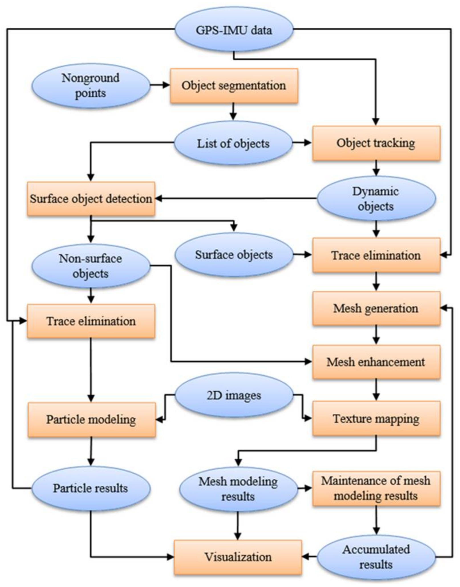
Figure 2.
Examples of vertical lines (red color) of some popular objects: (a) a wall; (b) a car; (c) a tree.
Figure 2.
Examples of vertical lines (red color) of some popular objects: (a) a wall; (b) a car; (c) a tree.
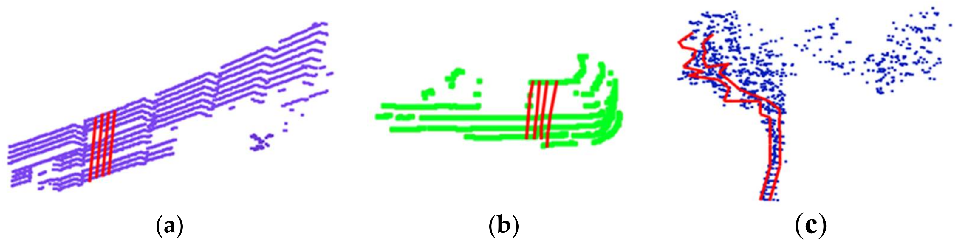
Figure 3.
Distortion values of the tree, car, and wall.
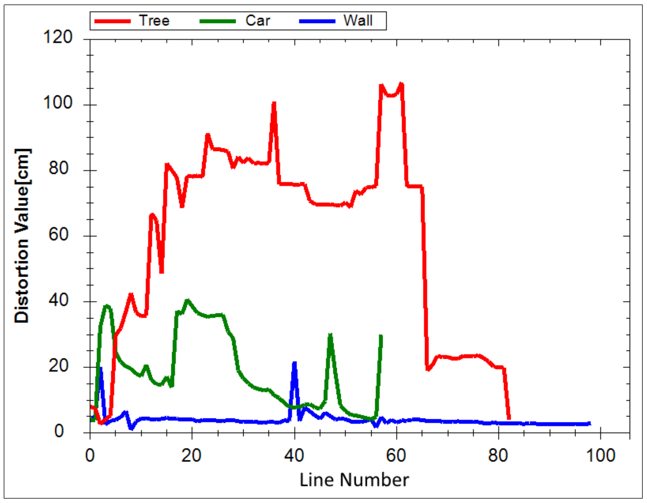
Figure 4.
Overview of the mesh generation method for surface objects.
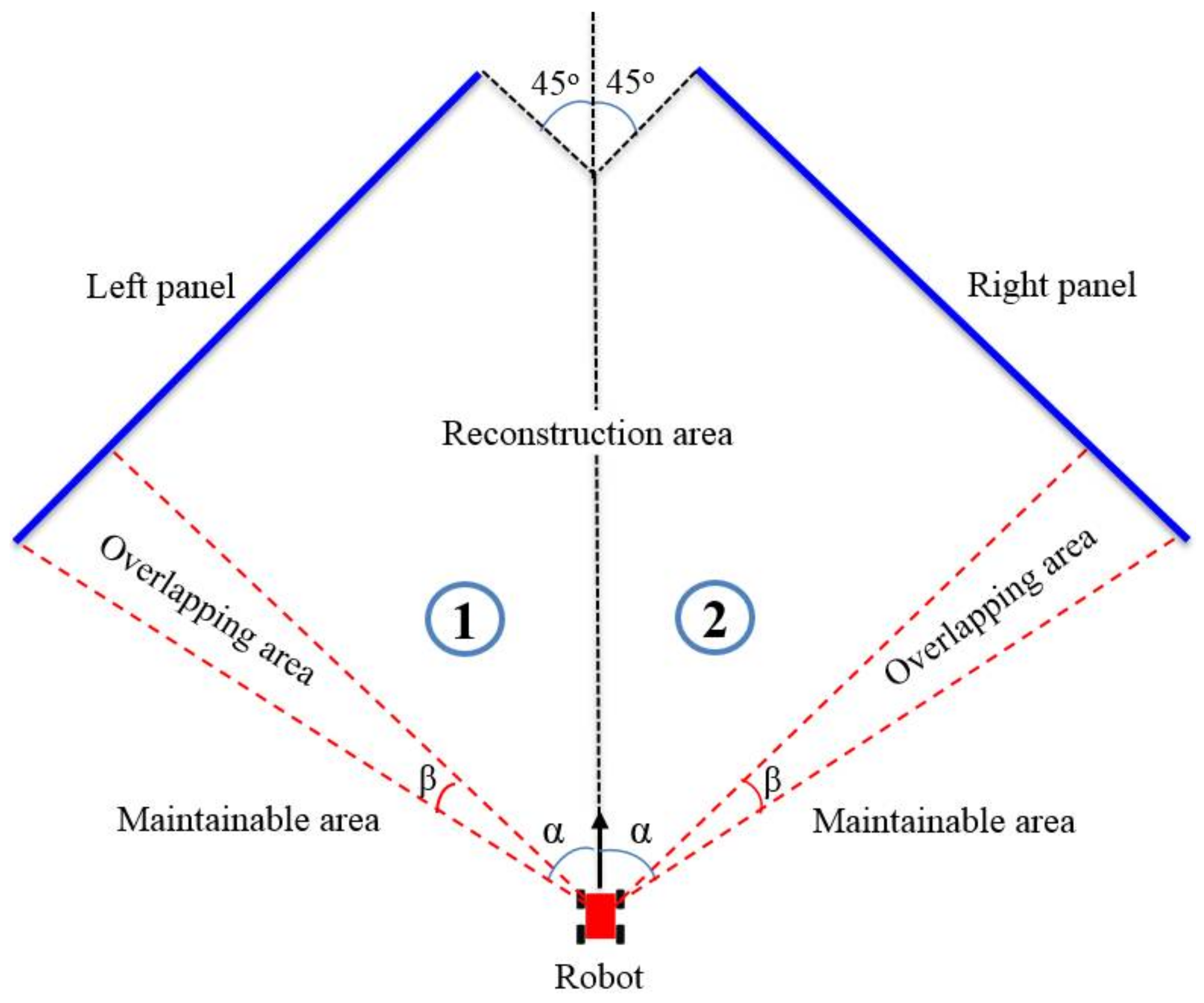
Figure 5.
Example of a sliding window for filling holes.
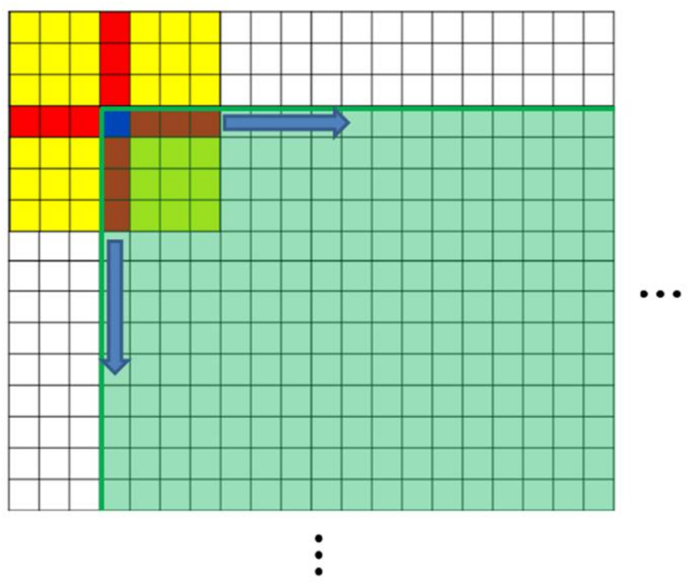
Figure 6.
Example of merging of particles near the surface meshes.
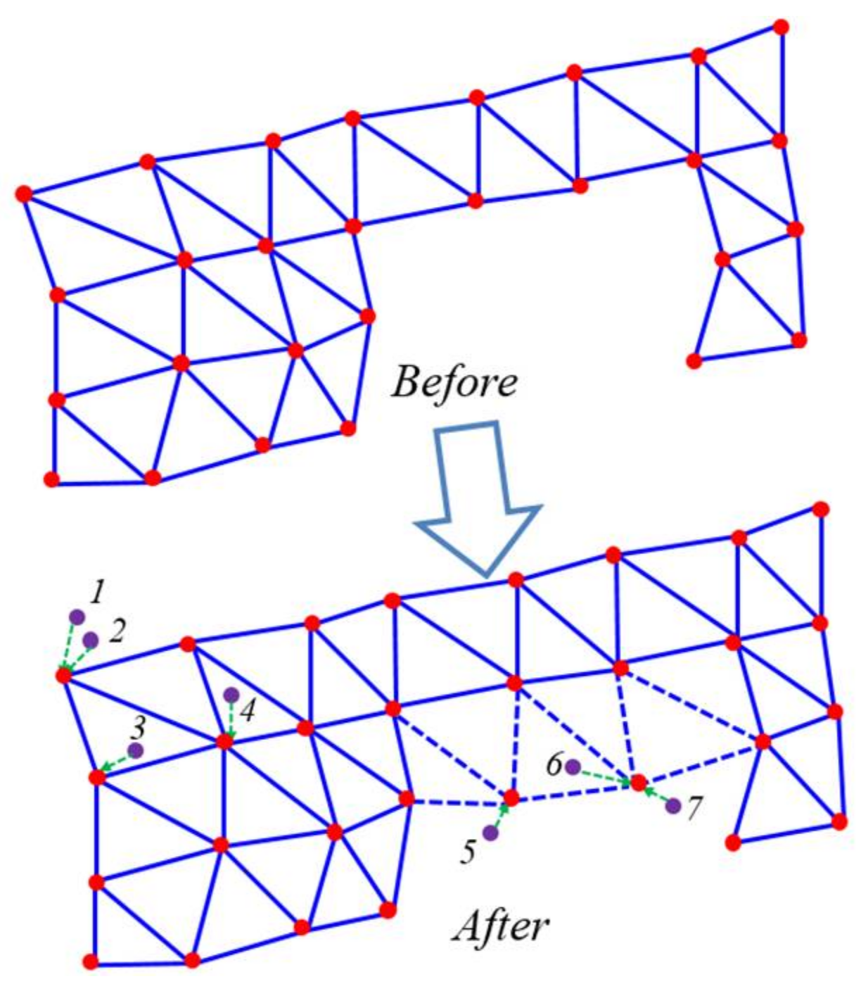
Figure 7.
Example of the meshes after enhancement.

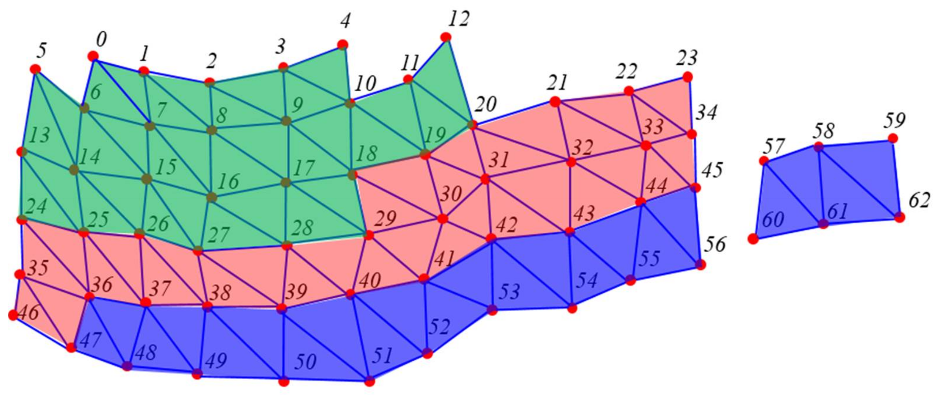
Figure 8.
Examples of vertex and index nodes.

Figure 9.
Example of texture nodes.
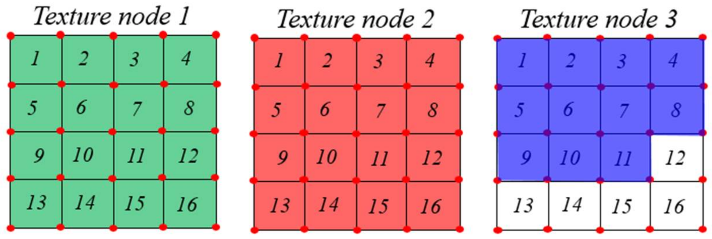
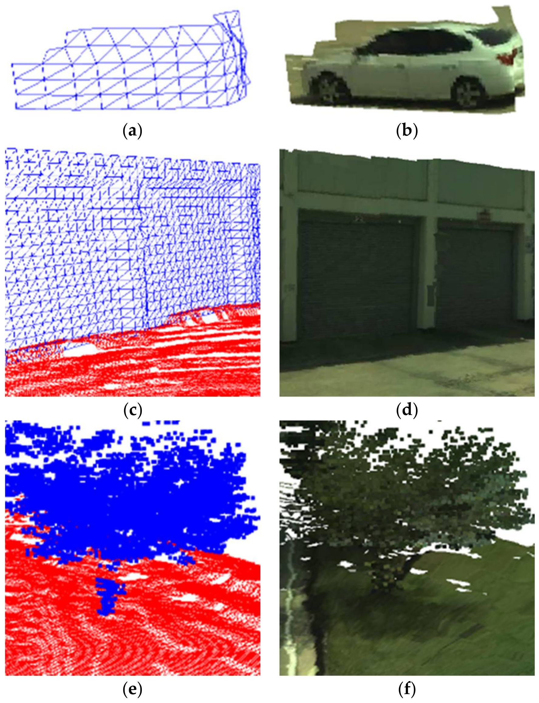
Figure 10.
Results of the proposed nonground modeling method for: (a,b) car (large dynamic object); (c,d) wall (surface object); (e,f) tree (non-surface object).
Figure 10.
Results of the proposed nonground modeling method for: (a,b) car (large dynamic object); (c,d) wall (surface object); (e,f) tree (non-surface object).

Figure 11.
Results of the full system in a static environment obtained using the proposed method for nonground modeling; and using an existing method [9] for ground modeling in: (a,b,d) suburban environments; (c) mountainous environment.
Figure 11.
Results of the full system in a static environment obtained using the proposed method for nonground modeling; and using an existing method [9] for ground modeling in: (a,b,d) suburban environments; (c) mountainous environment.
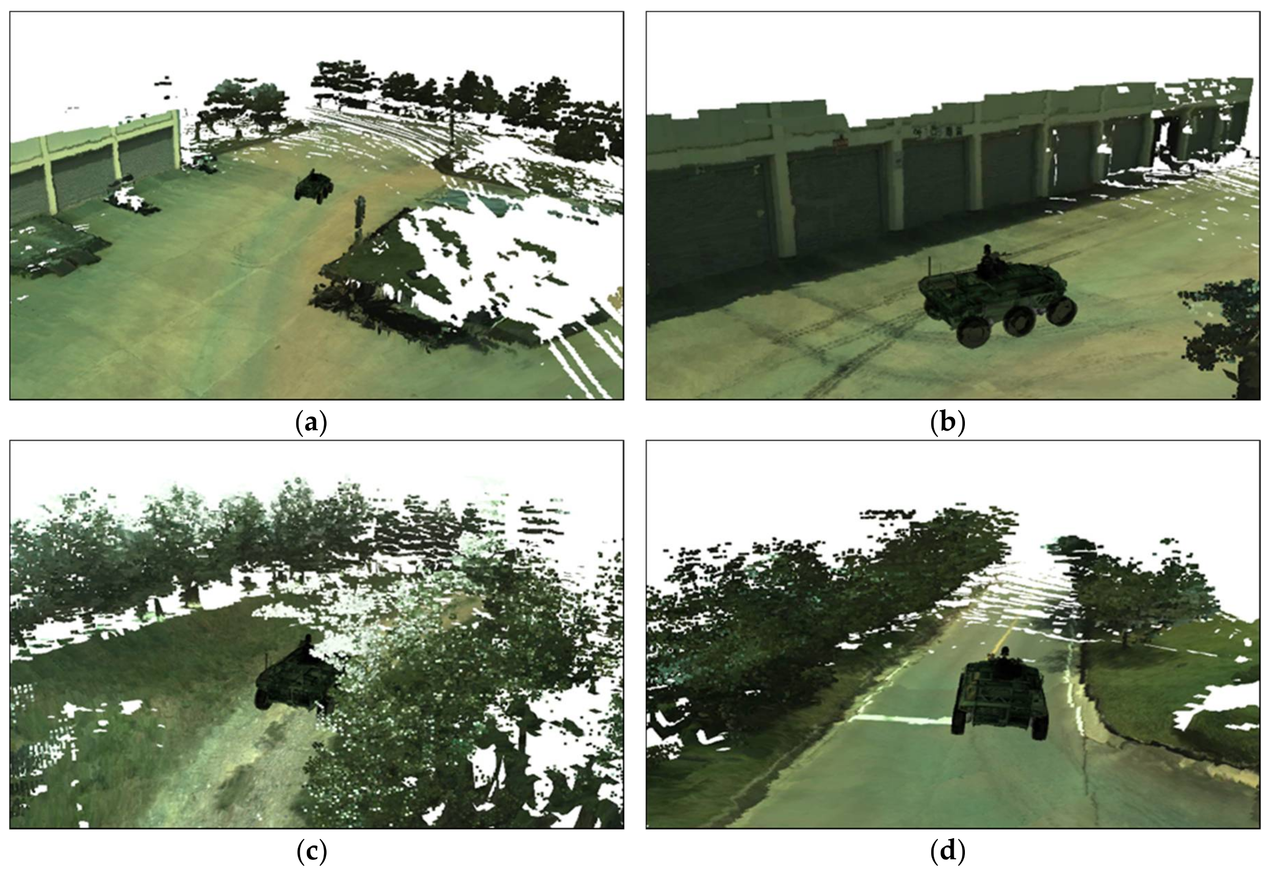
Figure 12.
Results of the full system in a dynamic environment obtained using the proposed method for nonground modeling, and using an existing method [9] for ground modeling: (a) two cars move across the robot in opposite directions; (b) two cars move along with and in front of the robot.
Figure 12.
Results of the full system in a dynamic environment obtained using the proposed method for nonground modeling, and using an existing method [9] for ground modeling: (a) two cars move across the robot in opposite directions; (b) two cars move along with and in front of the robot.
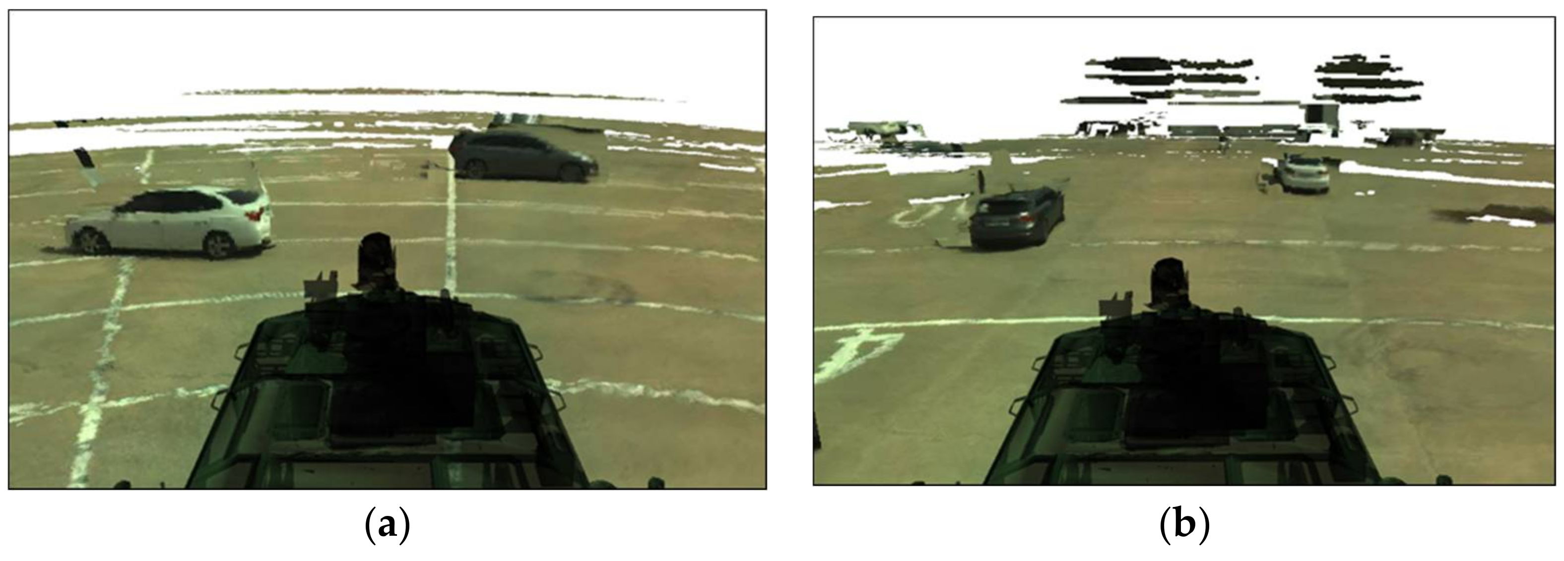
Figure 13.
Comparison of colored particle method [10,11,12] (a,c,e) and proposed method (b,d,f) for static surface objects.

Figure 14.
Comparison of colored particle method [10,11,12] (a,c,e) and proposed method (b,d,f) for large dynamic objects.

Figure 15.
Processing time per frame in: (a) surface object detection step; (b) colored particle modeling step; (c) mesh modeling step; (d) nonground modeling method.
Figure 15.
Processing time per frame in: (a) surface object detection step; (b) colored particle modeling step; (c) mesh modeling step; (d) nonground modeling method.


Table 1.
Average processing time of full modeling system.
| Step | Processing Time (ms) |
|---|---|
| Ground segmentation | 3.69 |
| Object segmentation | 4.56 |
| Object tracking | 0.34 |
| Surface object detection | 12.34 |
| Ground modeling | 43.7 |
| Nonground modeling | 28.98 |
| Total time | 93.61 |
© 2018 by the authors. Licensee MDPI, Basel, Switzerland. This article is an open access article distributed under the terms and conditions of the Creative Commons Attribution (CC BY) license (http://creativecommons.org/licenses/by/4.0/).
Share and Cite
MDPI and ACS Style
Chu, P.M.; Cho, S.; Sim, S.; Kwak, K.; Cho, K. Multimedia System for Real-Time Photorealistic Nonground Modeling of 3D Dynamic Environment for Remote Control System. Symmetry 2018, 10, 83. https://doi.org/10.3390/sym10040083
AMA Style
Chu PM, Cho S, Sim S, Kwak K, Cho K. Multimedia System for Real-Time Photorealistic Nonground Modeling of 3D Dynamic Environment for Remote Control System. Symmetry. 2018; 10(4):83. https://doi.org/10.3390/sym10040083
Chicago/Turabian StyleChu, Phuong Minh, Seoungjae Cho, Sungdae Sim, Kiho Kwak, and Kyungeun Cho. 2018. "Multimedia System for Real-Time Photorealistic Nonground Modeling of 3D Dynamic Environment for Remote Control System" Symmetry 10, no. 4: 83. https://doi.org/10.3390/sym10040083
Note that from the first issue of 2016, this journal uses article numbers instead of page numbers. See further details here.