The Cosine Measure of Single-Valued Neutrosophic Multisets for Multiple Attribute Decision-Making

Abstract

Based on the multiplicity evaluation in some real situations, this paper firstly introduces a single-valued neutrosophic multiset (SVNM) as a subclass of neutrosophic multiset (NM) to express the multiplicity information and the operational relations of SVNMs. Then, a cosine measure between SVNMs and weighted cosine measure between SVNMs are presented to measure the cosine degree between SVNMs, and their properties are investigated. Based on the weighted cosine measure of SVNMs, a multiple attribute decision-making method under a SVNM environment is proposed, in which the evaluated values of alternatives are taken in the form of SVNMs. The ranking order of all alternatives and the best one can be determined by the weighted cosine measure between every alternative and the ideal alternative. Finally, an actual application on the selecting problem illustrates the effectiveness and application of the proposed method.

1. Introduction

In 1965, Zadeh [1] proposed the theory of fuzzy sets (FS), in which every fuzzy element is expressed by the membership degree $T\left(x\right)$ belonging to the scope of [0, 1]. While the fuzzy membership degree of $T\left(x\right)$ is difficult to be determined, or cannot be expressed by an exact real number, the practicability of FS is limited. In order to avoid the above situation, Turksen [2] extended a single-value membership to an interval-valued membership. Generally, when the membership degree $T\left(x\right)$ is determined, the non-membership degree can be calculated by 1 − $T\left(x\right)$. Considering the role of the non-membership degree, Atanassov [3] put forward the intuitionistic fuzzy sets (IFS) and introduced the related theory of IFS. Since then, IFS has been widely used for solving the decision-making problems. Although the FS theory and IFS theory have been constantly extended and completed, they are not applicable to all the fuzzy problems. In 1998, Smarandache [4] added the uncertain degree to the IFS and put forward the theory of the neutrosophic set (NS), which is a general form of the FS and IFS. NS is composed of the neutrosophic components of truth, indeterminacy, and falsity denoted by T, I, F, respectively. Since then, many forms of the neutrosophic set were proposed as extensions of the neutrosophic set. Wang and Smarandache [5,6] introduced a single-valued neutrosophic set (SVNS) and an interval neutrosophic set (INS). Smarandache [7] and Smarandache and Ye [8] presented n-value and refined-single valued neutrosophic sets (R-SVNSs). Fan and Ye [9] presented a refined-interval neutrosophic set (R-INS). Ye [10] presented a dynamic single-valued neutrosophic multiset (DSVM), and so on.

Now, more researches have been done on the NS theory by experts and scholars. Ye [11,12] proposed the correlation coefficient and the weighted coefficient correlation of SVNS and proved that cosine similarity is a special case of the SVNS correlation coefficient. Broumi and Smarandache [13] proposed three vector similarity methods to simplify the similarity of SVNS, including Jaccard similarity, Dice similarity, and cosine similarity. Majumdar and Samanta [14] gave the similarity formula of SVNSs. Broumi and Smarandache [15] gave the correlation coefficient of INSs. Based on the Hamming and Euclidean distances, Ye [16] defined the similarity of INSs. For the operation rules of NSs, Smarandache, Ye, and Chi [4,16,17] gave different operation rules, respectively, where they all have certain rationality and applicability.

Recently, Smarandache [18] introduced the neutrosophic multiset and the neutrosophic multiset algebraic structures, in which one or more elements are repeated for some times, keeping the same or different neutrosophic components. Its concept is different from the concept of single-valued neutrosophic multiset in [10,19]. Until now, there are few studies and applications of neutrosophic multisets (NM) in science and engineering fields, so we introduce a single valued neutrosophic multiset (SVNM) as a subclass of the neutrosophic multiset (NM) to express the multiplicity information and propose a decision-making method based on the weighted cosine measures of SVNMs, and then provide a decision-making example to show its application under SVNM environments.

The remaining sections of this article are organized as follows. Section 2 describes some basic concepts of SVNS, NM, and the cosine measure of SVNSs. Section 3 presents a SVNM and its basic operational relations. Section 4 proposes a cosine measure between SVNMs and a weighted cosine measure between SVNMs and investigates their properties. Section 5 establishes a multiple attribute decision-making method using the weighted cosine measure of SVNMs under SVNM environment. Section 6 presents an actual example to demonstrate the application of the proposed methods under SVNM environment. Section 7 gives a conclusion and further research.

2. Some Concepts of SVNS and NM

Definition 1

[5]. Let X be a space of points (objects), with a generic element x in X. A SVNS R in X can be characterized by a truth-membership function$T_R\left(x\right)$, an indeterminacy-membership function$I_R\left(x\right)$, and a falsity-membership function$F_R\left(x\right)$, where$T_R\left(x\right),I_R\left(x\right),F_R\left(x\right)\in \left[0,1\right]$for each point x in X. Then, a SVNS R can be expressed by the following form:

$$R=\{\langle x,T_R\left(x\right),I_R\left(x\right),F_R\left(x\right)\rangle |x\in X\}.$$

Thus, the SVNS R satisfies the condition $0\le T_R\left(x\right)+I_R\left(x\right)+F_R\left(x\right)\le 3$.

For two SVNSs M and N, the relations of them are defined as follows [5]:

(1)

M ⊆ N if and only if $T_M\left(x\right)$ ≤ $T_N\left(x\right)$, $I_M\left(x\right)$ ≥ $I_N\left(x\right)$, $F_M\left(x\right)$ ≥ $F_N\left(x\right)$ for any x in X;

(2)

M = N if and only if M ⊆ N and N ⊆ M;

(3)

$M^c$ = {$\langle x,F_M\left(x\right), 1-I_M\left(x\right), T_M\left(x\right)\rangle |x\in X$}.

For writing convenience, an element called single-valued neutrosophic number (SVNN) in the SVNS R can be denoted by $R=\langle T_R\left(x\right),I_R\left(x\right),F_R\left(x\right)\rangle$ for any x in X. For two SVNNs M and N, the operational relations of them can be defined as follows [5]:

(1)

$M\cup N$ = <max$\left(T_M\left(x\right),T_N\left(x\right)\right)$, min$\left(I_M\left(x\right),I_N\left(x\right)\right)$, min$\left(F_M\left(x\right),F_N\left(x\right)\right)>$ for any x in X;

(2)

M ∩ N = <min$\left(T_M\left(x\right),T_N\left(x\right)\right)$, max$\left(I_M\left(x\right),I_N\left(x\right)\right)$, max$\left(F_M\left(x\right),F_N\left(x\right)\right)>$ for any x in X.

For two SVNNs M and N, the operational rules of them can be defined as follows [5]:

$$M+N=\langle T_M\left(x\right)+T_N\left(x\right)-T_M\left(x\right)T_N\left(x\right),I_M\left(x\right)I_N\left(x\right), F_M\left(x\right)F_N\left(x\right)\rangle \mathrm{for}\mathrm{any}x\mathrm{in}X;$$

(1)

$$M\times N=<T_M\left(x\right)T_N\left(x\right),I_M\left(x\right)+I_N\left(x\right)-I_M\left(x\right)I_N\left(x\right), F_M\left(x\right)+F_N\left(x\right)-F_M\left(x\right)F_N\left(x\right)>\mathrm{for}\mathrm{any} x \mathrm{in} X;$$

(2)

$$\phi M=<1-{\left(1-T_M\left(x\right)\right)}^{\phi },{\left(I_M\left(x\right)\right)}^{\phi },{\left(F_M\left(x\right)\right)}^{\phi }>\mathrm{for}\phi >0\mathrm{and}\mathrm{any}x\mathrm{in}X;$$

(3)

$$M^{\phi }=<{\left(T_M\left(x\right)\right)}^{\phi },{\left(1-I_M\left(x\right)\right)}^{\phi },{\left(1-F_M\left(x\right)\right)}^{\phi }>,\mathrm{for}\phi >0\mathrm{and}\mathrm{any}x\mathrm{in}X.$$

(4)

Definition 2

[20]. Let X $=\left\{x_1,x_2,\dots ,x_n\right\}$ be a space of points (objects), L and M be two SVNSs. The cosine measure between L and M is defined as follows:

$$\rho \left(L,M\right)=\frac{1}{n}{\sum }_{i=1}^{n}cos\{\frac{\pi }{6}(|T_L\left(x_i\right)-T_M\left(x_i\right)|+|I_L\left(x_i\right)-I_M\left(x_i\right)|+|F_L\left(x_i\right)-F_M\left(x_i\right)|)\}.$$

(5)

Obviously, the cosine measure between L and M satisfies the following properties [20]:

①

$0\le \rho \left(L,M\right)\le 1$;

②

$\rho \left(L,M\right)=1\mathrm{if}\mathrm{and}\mathrm{only}\mathrm{if} L=M;$

③

$\rho \left(L,M\right)=\rho \left(M,L\right)$.

Definition 3

[18]. Let X be a space of points (objects), and a neutrosophic multiset is repeated by one or more elements with the same or different neutrosophic components.

For example, M = $\left\{(m_1,\langle 0.7,0.2,0.1\rangle ),(m_2,\langle 0.6,0.4,0.1\rangle ),(m_3,\langle 0.8,0.3,0.2\rangle )\right\}$ is a neutrosophic set rather than a neutrosophic multiset; while K = {$(k_1,\langle 0.7,0.2,0.1\rangle ),(k_1,\langle 0.7,0.2,0.1\rangle ),(k_1\langle ,0.7,0.2,0.1\rangle ),(k_2,\langle 0.6,0.4,0.1\rangle )$} is a neutrosophic multiset, where the element $k_1$ is repeated. Then, we can say that the element $k_1$ has neutrosophic multiplicity 3 with the same neutrosophic components.

Meanwhile, L = {$(l_1,\langle 0.7,0.2,0.1\rangle ),(l_1,\langle 0.6,0.3,0.1\rangle ),(l_1,\langle 0.8,0.1,0.1\rangle ),(l_2,\langle 0.6,0.4,0.1\rangle )$} is also a neutrosophic multiset since the element $l_1$ is repeated, and then we can say that the element $l_1$ has neutrosophic multiplicity 3 with different neutrosophic components.

If the element $l_1$ is repeated times with the same neutrosophic comonents, we say $l_1$ has multiplicity. If the element $l_1$ is repeated times with different neutrosophic comonents, we say $l_1$ has the neutrosophic multiplicity ($nm$). The nm function can be defined as follows:

• $nm$: X→N = {1, 2, 3, …, ∞} for any $r\in R$
• $nm\left(r\right)$ = {$(p_1,\langle T_1,I_1,F_1\rangle ),(p_2,\langle T_2,I_2,F_2\rangle ),\dots ,(p_i,\langle T_i,I_i,F_i\rangle ),\dots$},

which means that r is repeated by $p_1$ times with the neutrosophic components $\langle T_1,I_1,F_1\rangle$; r is repeated by $p_2$ times with the neutrosophic components $\langle T_2,I_2,F_2\rangle$; …; r is repeated by $p_i$ times with the neutrosophic components $\langle T_i,I_i,F_i\rangle$; and so on. $p_1,p_2,\dots ,p_i,\dots \in N$, and $\langle T_j,I_j,F_j\rangle \ne \langle T_k,I_k,F_k\rangle$, for $j\ne k$ and $j, k\in N$. Then a neutrosophic multiset R can be written as:

$$\left(R,nm\left(r\right)\right) \mathrm{or}\left\{\left(r, nm\left(r\right), for r\in R\right)\right\}.$$

(6)

Now, with respect to the previous neutrosophic multisets K, L, we compute the neutrosophic multiplicity function:

• $n{m}_K:K\to N;$
• $n{m}_K\left(k_1\right)=\left\{(3,\langle 0.7,0.2,0.1\rangle )\right\}$;
• $n{m}_K\left(k_2\right)=\left\{\left(1,\langle 0.6,0.4,0.1\rangle \right)\right\};$
• $n{m}_L:L\to N$;
• $n{m}_L\left(l_1\right)=\left\{\left(1,\langle 0.7,0.2,0.1\rangle \right),\left(1,\langle 0.6,0.3,0.1\rangle \right),\left(1,\langle 0.8,0.1,0.1\rangle \right)\right\};$
• $n{m}_L\left(l_2\right)=\left\{\left(1,\langle 0.6,0.4,0.1\rangle \right)\right\}$.

3. Single Valued Neutrosophic Multiset

Definition 4.

Let X be a space of points (objects) with a generic element x in X and N = {1, 2, 3, …, ∞}. A SVNM R in X can be defined as follows:

$R=\{x,\left((p_{R1},\langle T_{R1}\left(x\right),I_{R1}\left(x\right),F_{R1}\left(x\right)\rangle ),(p_{R2},\langle T_{R2}\left(x\right),I_{R2}\left(x\right),F_{R2}\left(x\right)\rangle ),\dots ,(p_{Rj},\langle T_{Rj}\left(x\right),I_{Rj}\left(x\right),F_{Rj}\left(x\right)\rangle )\right)|x\in X\}$, where $T_{Rk}\left(x\right),I_{Rk}\left(x\right),F_{Rk}\left(x\right)$ express the truth-membership function, the indeterminacy-membership function, and the falsity-membership function, respectively. $T_{R1}\left(x\right),T_{R2}\left(x\right),\dots ,T_{Rk}\left(x\right)\in \left[0,1\right]$, $I_{R1}\left(x\right),I_{R2}\left(x\right),\dots ,I_{Rk}\left(x\right)\in \left[0,1\right],$ $F_{R1}\left(x\right),F_{R2}\left(x\right),\dots ,F_{Rk}\left(x\right)\in \left[0,1\right]$ and $0\le T_{Rk}\left(x\right)+I_{Rk}\left(x\right)+F_{Rk}\left(x\right)\le 3$, for k = 1, 2, …j, $j\in N$, $p_{R1},p_{R2},\dots ,p_{Rj}\in N$ and $p_{R1}+p_{R2}+\dots +p_{Rj}\ge 2$.

For convenience, a SVNM R can be denoted by the following simplified form:

$$R=\left\{x,(p_{Rk},\langle T_{Rk}\left(x\right),I_{Rk}\left(x\right),F_{Rk}\left(x\right)\rangle )|x\in X\right\},\hspace{1em}for k=1,2, \dots , j.$$

For example, with a universal set $X=\left\{x_1,x_2\right\},$ a SVNM R is given as:

$$R=\left\{\left(x_1,\left(2,\langle 0.6,0.2,0.1\rangle \right),\left(1,\langle 0.8,0.2,0.2\rangle \right)\right),\left(x_2,\left(1,\langle 0.7,0.3,0.1\rangle \right),\left(2,\langle 0.7,0.2,0.3\rangle \right)\right)\right\}.$$

Then

$$\begin{array}{c}n{m}_R\left(x_1\right)=\left\{\left(2,\langle 0.6,0.2,0.1\rangle \right),\left(1,\langle 0.8,0.2,0.2\rangle \right)\right\};\\ n{m}_R\left(x_2\right)=\left\{\left(1,\langle 0.7,0.3,0.1\rangle \right),\left(2,\langle 0.7,0.2,0.3\rangle \right)\right\}.\end{array}$$

Definition 5.

Let X be a space of points (objects) with a generic element x in X, M and L be two SVNMs,

$$M=\left\{x,(p_{Mk},\langle T_{Mk}\left(x\right),I_{Mk}\left(x\right),F_{Mk}\left(x\right)\rangle )|x\in X\right\}, for k=1, 2, \dots j,$$

$$L=\left\{x,(p_{Lk},\langle T_{Lk}\left(x\right),I_{Lk}\left(x\right),F_{Lk}\left(x\right)\rangle )|x\in X\right\},for k=1, 2, \dots j,$$

Then the relations of them are given as follows:

①

$M=L$, if and only if $p_{Mk}=p_{Lk},T_{Mk}\left(x\right)=T_{Lk}\left(x\right)$, $I_{Mk}\left(x\right)=I_{Lk}\left(x\right),F_{Mk}\left(x\right)=F_{Lk}\left(x\right), for k=1, 2, \dots , j;$

②

$M\cup L$ = $\{x,(\left(p_{Mk}\vee p_{Lk}\right),\langle T_{Mk}\left(x\right)\vee T_{Lk}\left(x\right),I_{Mk}\left(x\right)\wedge I_{Lk}\left(x\right),F_{Mk}\left(x\right)\wedge F_{Lk}\left(x\right)\rangle )|x\in X\},for k=1, 2,\dots , j$;

③

$M\cap L=\{x,(\left(p_{Mk}\wedge p_{Lk}\right),\langle T_{Mk}\left(x\right)\wedge T_{Lk}\left(x\right),I_{Mk}\left(x\right)\vee I_{Lk}\left(x\right),F_{Mk}\left(x\right)\vee F_{Lk}\left(x\right)\rangle )|x\in X\},for k=1, 2,\dots , j$.

For convenience, we can use $r=((p_{r1},<T_{r1}(x),I_{r1}(x),F_{r1}(x)>),(p_{r2},<T_{r2}(x),I_{r2}(x),F_{r2}(x)>),\dots ,(p_{rj},<T_{rj}(x),I_{rj}(x),F_{rj}(x)>))$ to express a basic element in a SVNM R and call r a single valued neutrosophic multiset element (SVNME).

For example, with a universal set $X=\{x_1,x_2\},$ then two SVNMs M and L are given as:

$$M=\left\{\left(x_1,\left(2,\langle 0.6,0.2,0.1\rangle \right),\left(1,\langle 0.4,0.1,0.2\rangle \right)\right),\left(x_2,(1,\langle 0.7,0.3,0.1\rangle )\right)\right\};$$

$$L=\left\{\left(x_1,\left(1,\langle 0.6,0.2,0.1\rangle \right),\left(1,\langle 0.8,0.2,0.1\rangle \right)\right),\left(x_2,\left(1,\langle 0.9,0.3,0.1\rangle \right)\right)\right\};$$

$$\begin{gathered} M\cup L=\{\left(x_1,\left(2,\langle 0.6,0.2,0.1\rangle \right),\left(1,\langle 0.4,0.1,0.2\rangle \right),\left(1,\langle 0.8,0.2,0.1\rangle \right)\right), \\ \left(x_2,\left(1,\langle 0.7,0.3,0.1\rangle \right),\left(1,\langle 0.9,0.3,0.1\rangle \right)\right)\} \end{gathered}$$

$$M\cap L=\left\{x_1,\left(1,\langle 0.6,0.2,0.1\rangle \right)\right\}.$$

Definition 6.

Let X be a space of points (objects) with a generic element x in X and M be a SVNM, we can change a SVNM M into a SVNS$\tilde{M}$by using the operational rules of SVNS.

$$M=\{x,\left(p_{Mk},\langle T_{Mk}\left(x\right),I_{Mk}\left(x\right),F_{Mk}\left(x\right)\rangle \right)|x\in X\},for k=1,2,\dots ,j.$$

Then

$$\tilde{M}=\{\langle x,1-{\prod }_{k=1}^j{\left(1-T_{Mk}\left(x\right)\right)}^{p_{Mk}},{\prod }_{k=1}^j{\left(I_{Mk}\left(x\right)\right)}^{p_{Mk}},{\prod }_{k=1}^j{\left(F_{Mk}\left(x\right)\right)}^{p_{Mk}}\rangle |x\in X\}.$$

(7)

Proof. 

 

Set $m_1,m_2,\dots m_j$ are basic elements in M.

When k = 1, we can get

$m_1=(\langle T_{m1}\left(x\right),I_{m1}\left(x\right),F_{m1}\left(x\right)\rangle ,\langle T_{m1}\left(x\right),I_{m1}\left(x\right),F_{m1}\left(x\right)\rangle ,\dots ,\langle T_{m1}\left(x\right),I_{m1}\left(x\right),F_{m1}\left(x\right)\rangle )$, which has neutrosophic multiplicity $p_{m1}$.

According to the operational rules of SVNSs, we can get:

$$+m_1=1-{\left(1-T_{m1}\left(x\right)\right)}^{p_{m1}},{\left(I_{m1}\left(x\right)\right)}^{p_{m1}},{\left(F_{m1}\left(x\right)\right)}^{p_{m1}}.$$

As the same reason, when k = 2, we can get

$$+m_2=1-{\left(1-T_{m2}\left(x\right)\right)}^{p_{m2}},{\left(I_{m1}\left(x\right)\right)}^{p_{m2}},{\left(F_{m2}\left(x\right)\right)}^{p_{m2}}.$$

Then

$$\begin{gathered} m_1+m_2=1-{\left(1-T_{m1}\left(x\right)\right)}^{p_{m1}}{\left(1-T_{m2}\left(x\right)\right)}^{p_{m2}},{\left(I_{m1}\left(x\right)\right)}^{p_{m1}}{\left(I_{m1}\left(x\right)\right)}^{p_{m2}},{\left(F_{m2}\left(x\right)\right)}^{p_{m1}}{\left(F_{m2}\left(x\right)\right)}^{p_{m2}} \\ =1-{\prod }_{k=1}^2{\left(1-T_{mk}\left(x\right)\right)}^{p_{mk}},{\prod }_{k=1}^2{\left(I_{mk}\left(x\right)\right)}^{p_{mk}},{\prod }_{k=1}^2{\left(F_{mk}\left(x\right)\right)}^{p_{mk}}; \end{gathered}$$

Suppose when k = i, the Equation (7) is established, then we can get:

$$m_1+m_2+\dots +m_i=1-{\prod }_{k=1}^i{(-T_{mk}\left(x\right))}^{p_{mk}},{\prod }_{k=1}^i{\left(I_{mk}\left(x\right)\right)}^{p_{mk}},{\prod }_{k=1}^i{\left(F_{mk}\left(x\right)\right)}^{p_{mk}};$$

Then

$$\begin{array}{cc}\hfill m_1+m_2+\dots +m_i& +m_{i+1}\hfill \\ & =1-{\displaystyle \prod _{k=1}^i}{\left(1-T_{mk}\left(x\right)\right)}^{p_{mk}}+1-{\left(1-T_{m\left(i+1\right)}\left(x\right)\right)}^{p_{m\left(i+1\right)}}\hfill \\ & -\left(1-{\displaystyle \prod _{k=1}^i}{\left(1-T_{mk}\left(x\right)\right)}^{p_{mk}}\right)\left(1-{\left(1-T_{m\left(i+1\right)}\left(x\right)\right)}^{p_{m\left(i+1\right)}}\right),\hfill \\ & \left({\displaystyle \prod _{k=1}^i}{\left(I_{mk}\left(x\right)\right)}^{p_{mk}}\right){\left(I_{m\left(i+1\right)}\left(x\right)\right)}^{p_{m\left(i+1\right)}},\hfill \\ & \left({\displaystyle \prod _{k=1}^i}{\left(F_{mk}\left(x\right)\right)}^{p_{mk}}\right){\left(F_{m\left(i+1\right)}\left(x\right)\right)}^{p_{m\left(i+1\right)}}\hfill \\ & =1-{\prod }_{k=1}^{i+1}{\left(1-T_{mk}\left(x\right)\right)}^{p_{mk}},{\prod }_{k=1}^{i+1}{\left(I_{mk}\left(x\right)\right)}^{p_{mk}},{\prod }_{k=1}^{i+1}{\left(F_{mk}\left(x\right)\right)}^{p_{mk}}.\hfill \end{array}$$

To sum up, when k = i + 1, Equation (7) is true, and then according to the mathematical induction, we can get that the aggregation result is also true. ☐

Definition 7.

Let $X=\left\{x_1,x_2,\dots ,x_n\right\}$ be a universe of discourse, and M and N be two SVNMs, and then the operational rules of SVNMs are defined as follows:

$$M=\left\{x,(p_{Mk},\langle T_{Mk}\left(x\right),I_{Mk}\left(x\right),F_{Mk}\left(x\right)\rangle )|x\in X\right\}, for k=1, 2,\dots j;$$

$$N=\left\{x,(p_{Nk},\langle T_{Nk}\left(x\right),I_{Nk}\left(x\right),F_{Nk}\left(x\right)\rangle )|x\in X\right\},for k=1, 2,\dots j ;$$

$$\begin{array}{c}M\oplus N\hfill \\ =\{\langle x,1\hfill \\ -{\displaystyle \prod _{k=1}^j}{\left(1-T_{Mk}\left(x\right)\right)}^{p_{Mk}}{\displaystyle \prod _{k=1}^j}(1\hfill \\ {-T_{Nk}\left(x\right))}^{p_{Nk}},{\displaystyle \prod _{k=1}^j}{\left(I_{Mk}\left(x\right)\right)}^{p_{Mk}}{\displaystyle \prod _{k=1}^j}{\left(I_{Nk}\left(x\right)\right)}^{p_{Nk}},{\displaystyle \prod _{k=1}^j}{\left(F_{Mk}\left(x\right)\right)}^{p_{Mk}}{\displaystyle \prod _{k=1}^j}{\left(F_{Nk}\left(x\right)\right)}^{p_{Nk}}\rangle |x\in X\}\hfill \end{array}$$

$$\begin{array}{ccc}\hfill M\otimes N& =& \{\langle x,(1-{\displaystyle \prod _{k=1}^j}{\left(1-T_{Mk}\left(x\right)\right)}^{p_{Mk}}\left)\right(1-{\displaystyle \prod _{k=1}^j}{\left(1-T_{Nk}\left(x\right)\right)}^{p_{Nk}}),{\displaystyle \prod _{k=1}^j}{\left(I_{Mk}\left(x\right)\right)}^{p_{Mk}}\\ & & +{\displaystyle \prod _{k=1}^j}{\left(I_{Nk}\left(x\right)\right)}^{p_{Nk}}-{\displaystyle \prod _{k=1}^j}{\left(I_{Mk}\left(x\right)\right)}^{p_{Mk}}{\displaystyle \prod _{k=1}^j}{\left(I_{Nk}\left(x\right)\right)}^{p_{Nk}},{\displaystyle \prod _{k=1}^j}{\left(F_{Mk}\left(x\right)\right)}^{p_{Mk}}\hfill \\ & & +{\displaystyle \prod _{k=1}^j}{\left(F_{Nk}\left(x\right)\right)}^{p_{Nk}}-{\displaystyle \prod _{k=1}^j}{\left(F_{Mk}\left(x\right)\right)}^{p_{Mk}}{\displaystyle \prod _{k=1}^j}{\left(F_{Nk}\left(x\right)\right)}^{p_{Nk}}\rangle |x\in X\}\hfill \end{array}$$

$$\phi M=\{\langle x,\left(1-{\left({\displaystyle \prod _{k=1}^j}{\left(1-T_{Mk}\left(x\right)\right)}^{p_{Mk}}\right)}^{\phi }\right),{\left({\displaystyle \prod _{k=1}^j}{\left(I_{Mk}\left(x\right)\right)}^{p_{Mk}}\right)}^{\phi },{\left({\displaystyle \prod _{k=1}^j}{\left(F_{Nk}\left(x\right)\right)}^{p_{Nk}}\right)}^{\phi }\rangle |x\in X\}$$

$$\begin{array}{c}{M}^{\phi }=\{\langle x,{\left(1-{\displaystyle \prod _{k=1}^j}{\left(1-T_{Mk}\left(x\right)\right)}^{p_{Mk}}\right)}^{\phi },1-{\left(1-{\displaystyle \prod _{k=1}^j}{\left(I_{Mk}\left(x\right)\right)}^{p_{Mk}}\right)}^{\phi },1\\ -{\left(1-{\displaystyle \prod _{k=1}^j}{\left(F_{Nk}\left(x\right)\right)}^{p_{Nk}}\right)}^{\phi }\rangle |x\in X\}\end{array}$$

4. Cosine Measures of Single-Value Neutrosophic Multisets

Cosine measures are usually used in science and engineering applications. In this section, we propose a cosine measure of SVNMs and a weighted cosine measure of SVNMs.

Definition 8.

Let $X=\left\{x_1,x_2,\dots ,x_n\right\}$ be a universe of discourse, M and N be two SVNMs,

$$M=\{x_i,\left(p_{M1},\langle T_{M1}\left(x_i\right),I_{M1}\left(x_i\right),F_{M1}\left(x_i\right)\rangle \right),\left(p_{M2},\langle T_{M2}\left(x_i\right),I_{M2}\left(x_i\right),F_{M2}\left(x_i\right)\rangle \right),\dots ,\left(p_{Mj},\langle T_{Mj}\left(x_i\right),I_{Mj}\left(x_i\right),F_{Mj}\left(x_i\right)\rangle \right)|x_i\in X\},$$

$$N=\left\{\begin{array}{c}{x}_i,\left(p_{N1},\langle T_{N1}\left(x_i\right),I_{N1}\left(x_i\right),F_{N1}\left(x_i\right)\rangle \right),\left(p_{N2},\langle T_{N2}\left(x_i\right),I_{N2}\left(x_i\right),F_{N2}\left(x_i\right)\rangle \right),\dots ,\left(p_{Nj},\langle T_{Nj}\left(x_i\right),I_{Nj}\left(x_i\right),F_{Nj}\left(x_i\right)\rangle \right)\end{array}\right|x_i\in X\}$$

Then, a cosine measure between two SVNMs M and N is defined as follows:

$$\begin{array}{ccc}\hfill \rho (M,N)& =& \frac{1}{n}{\displaystyle \sum _{i=1}^n}cos\left\{\frac{\pi }{6}\right|{\displaystyle \prod _{k=1}^j}{\left(1-T_{Mk}\left(x_i\right)\right)}^{p_{Mk}}-{\displaystyle \prod _{k=1}^j}{\left(1-T_{Nk}\left(x_i\right)\right)}^{p_{Nk}}|\hfill \\ & & +\left|{\displaystyle \prod _{k=1}^j}{\left(I_{Mk}\left(x_i\right)\right)}^{p_{Mk}}-{\displaystyle \prod _{k=1}^j}{\left(I_{Nk}\left(x_i\right)\right)}^{p_{Nk}}\right|\hfill \\ & & +|{\displaystyle \prod _{k=1}^j}{\left(F_{Mk}\left(x_i\right)\right)}^{p_{Mk}}-{\displaystyle \prod _{k=1}^j}{\left(F_{Nk}\left(x_i\right)\right)}^{p_{Nk}}|\}\hfill \end{array}$$

(8)

Theorem 1.

The cosine measure $\rho \left(M,N\right)$ between two SVNMs M and N satisfies the following properties:

①

$\rho \left(M,N\right)=\rho \left(N,M\right)$;

②

$0\le \rho \left(M,N\right)\le 1$;

③

$\rho \left(M,N\right)=1,if and only if M=N.$

Proof. 

 

①:

For $\left|{\prod }_{k=1}^j{\left(1-T_{Mk}\left(x_i\right)\right)}^{p_{Mk}}-{\prod }_{k=1}^j{\left(1-T_{Nk}\left(x_i\right)\right)}^{p_{Nk}}\right|+\left|{\prod }_{k=1}^j{\left(I_{Mk}\left(x_i\right)\right)}^{p_{Mk}}-{\prod }_{k=1}^j{\left(I_{Nk}\left(x_i\right)\right)}^{p_{Nk}}\right|+\left|{\prod }_{k=1}^j{\left(F_{Mk}\left(x_i\right)\right)}^{p_{Mk}}-{\prod }_{k=1}^j{\left(F_{Nk}\left(x_i\right)\right)}^{p_{Nk}}\right|=\left|{\prod }_{k=1}^j{\left(1-T_{Nk}\left(x_i\right)\right)}^{p_{Nk}}-{\prod }_{k=1}^j{\left(1-T_{Mk}\left(x_i\right)\right)}^{p_{Mk}}\right|+\left|{\prod }_{k=1}^j{\left(I_{Nk}\left(x_i\right)\right)}^{p_{Nk}}-{\prod }_{k=1}^j{\left(I_{Mk}\left(x_i\right)\right)}^{p_{Mk}}\right|+\left|{\prod }_{k=1}^j{\left(F_{Nk}\left(x_i\right)\right)}^{p_{Nk}}-{\prod }_{k=1}^j{\left(F_{Mk}\left(x_i\right)\right)}^{p_{Mk}}\right|$, so we can get $\rho \left(M,N\right)=\rho \left(N,M\right)$.

②:

For $0\le T_{Mk}\left(x_i\right)\le 1, 0\le I_{Mk}\left(x_i\right)\le 1, 0\le F_{Mk}\left(x_i\right)\le 1,0\le T_{Nk}\left(x_i\right)\le 1, 0\le I_{Nk}\left(x_i\right)\le 1, 0\le F_{Nk}\left(x_i\right)\le 1;$

Then, we can get

$$0\le 1-T_{Mk}\left(x_i\right)\le 1 and 0\le 1-T_{Nk}\left(x_i\right)\le 1;$$

$$0\le {\prod }_{k=1}^j{\left(1-T_{Mk}\left(x_i\right)\right)}^{p_{Mk}}\le 1 and 0\le {\prod }_{k=1}^j{\left(1-T_{Nk}\left(x_i\right)\right)}^{p_{Nk}}\le 1;$$

So,

$$0\le \left|{\prod }_{k=1}^j{\left(1-T_{Mk}\left(x_i\right)\right)}^{p_{Mk}}-{\prod }_{k=1}^j{\left(1-T_{Nk}\left(x_i\right)\right)}^{p_{Nk}}\right|\le 1.$$

 ☐.

For the same reason, we can get

$$\begin{array}{c}0\le \left|{\displaystyle \prod _{k=1}^j}{\left(I_{Mk}\left(x_i\right)\right)}^{p_{Mk}}-{\displaystyle \prod _{k=1}^j}{\left(I_{Nk}\left(x_i\right)\right)}^{p_{Nk}}\right|\le 1\hspace{1em}and\hspace{1em}0\hfill \\ \hfill \le \left|{\displaystyle \prod _{k=1}^j}{\left(F_{Mk}\left(x_i\right)\right)}^{p_{Mk}}-{\displaystyle \prod _{k=1}^j}{\left(F_{Nk}\left(x_i\right)\right)}^{p_{Nk}}\right|\le 1\end{array}$$

Above all, we can get $0\le \left|{\prod }_{k=1}^j{\left(1-T_{Mk}\left(x_i\right)\right)}^{p_{Mk}}-{\prod }_{k=1}^j{\left(1-T_{Nk}\left(x_i\right)\right)}^{p_{Nk}}\right|+\left|{\prod }_{k=1}^j{\left(I_{Mk}\left(x_i\right)\right)}^{p_{Mk}}-{\prod }_{k=1}^j{\left(I_{Nk}\left(x_i\right)\right)}^{p_{Nk}}\right|+\left|{\prod }_{k=1}^j{\left(F_{Mk}\left(x_i\right)\right)}^{p_{Mk}}-{\prod }_{k=1}^j{\left(F_{Nk}\left(x_i\right)\right)}^{p_{Nk}}\right|\le 3$ and $0\le {\sum }_{i=1}^{n}cos\left\{\frac{\pi }{6}\right|{\prod }_{k=1}^j{\left(1-T_{Mk}\left(x_i\right)\right)}^{p_{Mk}}-{\prod }_{k=1}^j{\left(1-T_{Nk}\left(x_i\right)\right)}^{p_{Nk}}|+\left|{\prod }_{k=1}^j{\left(I_{Mk}\left(x_i\right)\right)}^{p_{Mk}}-{\prod }_{k=1}^j{\left(I_{Nk}\left(x_i\right)\right)}^{p_{Nk}}\right|+\left|{\prod }_{k=1}^j{\left(F_{Mk}\left(x_i\right)\right)}^{p_{Mk}}-{\prod }_{k=1}^j{\left(F_{Nk}\left(x_i\right)\right)}^{p_{Nk}}\right|\}\le 1;$

$$\begin{array}{l}\rho (M,N)=\frac{1}{n}{\displaystyle \sum _{i=1}^n}cos\left\{\frac{\pi }{6}\right|{\displaystyle \prod _{k=1}^j}{\left(1-T_{Mk}\left(x_i\right)\right)}^{p_{Mk}}-{\displaystyle \prod _{k=1}^j}{\left(1-T_{Nk}\left(x_i\right)\right)}^{p_{Nk}}|\\ +\left|{\displaystyle \prod _{k=1}^j}{\left(I_{Mk}\left(x_i\right)\right)}^{p_{Mk}}-{\displaystyle \prod _{k=1}^j}{\left(I_{Nk}\left(x_i\right)\right)}^{p_{Nk}}\right|\\ +|{\displaystyle \prod _{k=1}^j}{\left(F_{Mk}\left(x_i\right)\right)}^{p_{Mk}}-{\displaystyle \prod _{k=1}^j}{\left(F_{Nk}\left(x_i\right)\right)}^{p_{Nk}}|\}\\ =\frac{1}{n}\left(cos\right\{\frac{\pi }{6}(\left|{\displaystyle \prod _{k=1}^j}{\left(1-T_{Mk}\left(x_1\right)\right)}^{p_{Mk}}-{\displaystyle \prod _{k=1}^j}{\left(1-T_{Nk}\left(x_1\right)\right)}^{p_{Nk}}\right|\\ +\left|{\displaystyle \prod _{k=1}^j}{\left(I_{Mk}\left(x_1\right)\right)}^{p_{Mk}}-{\displaystyle \prod _{k=1}^j}{\left(I_{Nk}\left(x_1\right)\right)}^{p_{Nk}}\right|\\ +\left|{\displaystyle \prod _{k=1}^j}{\left(F_{Mk}\left(x_1\right)\right)}^{p_{Mk}}-{\displaystyle \prod _{k=1}^j}{\left(F_{Nk}\left(x_1\right)\right)}^{p_{Nk}}\right|\left)\right\}\\ +cos\left\{\frac{\pi }{6}\right(\left|{\displaystyle \prod _{k=1}^j}{\left(1-T_{Mk}\left(x_2\right)\right)}^{p_{Mk}}-{\displaystyle \prod _{k=1}^j}{\left(1-T_{Nk}\left(x_2\right)\right)}^{p_{Nk}}\right|\\ +\left|{\displaystyle \prod _{k=1}^j}{\left(I_{Mk}\left(x_2\right)\right)}^{p_{Mk}}-{\displaystyle \prod _{k=1}^j}{\left(I_{Nk}\left(x_2\right)\right)}^{p_{Nk}}\right|\\ +\left|{\displaystyle \prod _{k=1}^j}{\left(F_{Mk}\left(x_2\right)\right)}^{p_{Mk}}-{\displaystyle \prod _{k=1}^j}{\left(F_{Nk}\left(x_2\right)\right)}^{p_{Nk}}\right|\left)\right\}+\dots \\ +cos\left\{\frac{\pi }{6}\right(\left|{\displaystyle \prod _{k=1}^j}{\left(1-T_{Mk}\left(x_n\right)\right)}^{p_{Mk}}-{\displaystyle \prod _{k=1}^j}{\left(1-T_{Nk}\left(x_n\right)\right)}^{p_{Nk}}\right|\\ +\left|{\displaystyle \prod _{k=1}^j}{\left(I_{Mk}\left(x_n\right)\right)}^{p_{Mk}}-{\displaystyle \prod _{k=1}^j}{\left(I_{Nk}\left(x_n\right)\right)}^{p_{Nk}}\right|\\ +\left|{\displaystyle \prod _{k=1}^j}{\left(F_{Mk}\left(x_n\right)\right)}^{p_{Mk}}-{\displaystyle \prod _{k=1}^j}{\left(F_{Nk}\left(x_n\right)\right)}^{p_{Nk}}\right|\left)\right\})\end{array}$$

Let $cos\left\{\frac{\pi }{6}\right(\left|{\prod }_{k=1}^j{\left(1-T_{Mk}\left(x_i\right)\right)}^{p_{Mk}}-{\prod }_{k=1}^j{\left(1-T_{Nk}\left(x_i\right)\right)}^{p_{Nk}}\right|+\left|{\prod }_{k=1}^j{\left(I_{Mk}\left(x_i\right)\right)}^{p_{Mk}}-{\prod }_{k=1}^j{\left(I_{Nk}\left(x_i\right)\right)}^{p_{Nk}}\right|+\left|{\prod }_{k=1}^j{\left(F_{Nk}\left(x_i\right)\right)}^{p_{Mk}}-{\prod }_{k=1}^j{\left(F_{Nk}\left(x_i\right)\right)}^{p_{Nk}}\right|\left)\right\}=a_i(i=1,2,\dots n)$, then $\rho \left(M,N\right)=\frac{1}{n}\{a_1+a_2+\dots +a_n$}.

According to $0\le cos\left\{\frac{\pi }{6}\left(\left|{\prod }_{k=1}^j{\left(1-T_{Mk}\left(x_i\right)\right)}^{p_{Mk}}-{\prod }_{k=1}^j{\left(1-T_{Nk}\left(x_i\right)\right)}^{p_{Nk}}\right|+\left|{\prod }_{k=1}^j{\left(I_{Mk}\left(x_i\right)\right)}^{p_{Mk}}-{\prod }_{k=1}^j{\left(I_{Nk}\left(x_i\right)\right)}^{p_{Nk}}\right|+\left|{\prod }_{k=1}^j{\left(F_{Mk}\left(x_i\right)\right)}^{p_{Mk}}-{\prod }_{k=1}^j{\left(F_{Nk}\left(x_i\right)\right)}^{p_{Nk}}\right|\right)\right\}=a_i\le 1$, we can obtain $0\le a_1+a_2+\dots +a_n\le n$ and $0\le \frac{1}{n}\left(a_1+a_2+\dots +a_n\right)\le 1$, so we can get $0\le \rho \left(M,N\right)\le 1$.

③ If M = N then $T_{Mk}\left(x_i\right)=T_{Nk}\left(x_i\right),I_{Mk}\left(x_i\right)=I_{Nk}\left(x_i\right),and{F}_{Mk}\left(x_i\right)=F_{Nk}\left(x_i\right)$ for any $x_i\in Xandi=1,2,\dots n,$ so we can get $\rho \left(M,N\right)=1,\mathrm{if}\mathrm{and}\mathrm{only}\mathrm{if}M=N$.

Now, we consider different weights for each element $x_i\left(i=1,2,\dots ,n\right)$ in X. Then, let $w={\left(w_1,w_2,\dots ,w_n\right)}^T$ be the weight vector of each element $x_i\left(i=1,2,\dots ,n\right)\mathrm{with}{w}_i\in \left[0,1\right],$ and ${\sum }_{i=1}^n{w}_i=1$. Hence, we further extend the cosine measure of Equation (8) to the following weighted cosine measure of SVNM:

$$\begin{array}{l}{\rho }_w(M,N)={\displaystyle \sum _{i=1}^n}{w}_{i}cos\left\{\frac{\pi }{6}\right(|{\displaystyle \prod _{k=1}^j}{\left(1-T_{Mk}\left(x_i\right)\right)}^{p_{Mk}}-{\displaystyle \prod _{k=1}^j}{\left(1-T_{Nk}\left(x_i\right)\right)}^{p_{Nk}}|\\ +\left|{\displaystyle \prod _{k=1}^j}{\left(I_{Mk}\left(x_i\right)\right)}^{p_{Mk}}-{\displaystyle \prod _{k=1}^j}{\left(I_{Nk}\left(x_i\right)\right)}^{p_{Nk}}\right|\\ +|{\displaystyle \prod _{k=1}^j}{\left(F_{Mk}\left(x_i\right)\right)}^{p_{Mk}}-{\displaystyle \prod _{k=1}^j}{\left(F_{Nk}\left(x_i\right)\right)}^{p_{Nk}}|\left)\right\}\end{array}$$

(9)

Theorem 2.

The cosine measure ${\rho }_w\left(M,N\right)$ between two SVNMs M and N satisfies the following properties:

①

${\rho }_w\left(M,N\right)={\rho }_w\left(N,M\right)$;

②

$0\le {\rho }_w\left(M,N\right)\le 1$;

③

${\rho }_w\left(M,N\right)=1,if and only if M=N.$

The proof of Theorem 2 is similar to that of the Theorem 1, so we omitted it here.

5. Cosine Measure of SVNM for Multiple Attribute Decision-Making

In this section, we use the weighted cosine measure of SVNM to deal with the multiple attribute decision-making problems with SVNM information.

Let $G=\left\{g_1,g_2,\dots , g_m\right\}$ as a set of alternatives and $X=\left\{x_1,x_2,\dots , x_n\right\}$ as a set of attributes, then they can be established in a decision-making problem. However, sometimes $x_i\left(i=1, 2,\dots ,n\right)$ may have multiplicity, and then we can use the form of a SVNM to represent the evaluation value.

Let $g_r=\begin{array}{c}\{x_i,(p_{g_{r}1},\langle T_{g_{r}1}\left(x_i\right),I_{g_{r}1}\left(x_i\right),F_{g_{r}1}\left(x_i\right)\rangle ),\left(p_{g_{r}2},\langle T_{g_{r}2}\left(x_i\right),I_{g_{r}2}\left(x_i\right),F_{g_{r}2}\left(x_i\right)\rangle \right),\dots ,\left(p_{g_{r}j},\langle T_{g_{r}j}\left(x_i\right),I_{g_{r}j}\left(x_i\right),F_{g_{r}j}\left(x_i\right)\rangle \right)\end{array}|x_i\in X\}$, for r = 1, 2, …, m and i = 1, 2, …, n. Then we can establish the SVNM decision matrix D, which is shown in

Table 1. The single-valued neutrosophic multiset (SVNM) decision matrix D.

	${\mathit{x}}_{\mathbf{1}}$	$\dots$
$g_1$	$x_1,\left(p_{g_{1}1},\langle T_{g_{1}1}\left(x_1\right),I_{g_{1}1}\left(x_1\right),F_{g_{1}1}\left(x_1\right)\rangle \right),\dots ,\left(p_{g_{1}j},\langle T_{g_{1}j}\left(x_1\right),I_{g_{1}j}\left(x_1\right),F_{g_{1}j}\left(x_1\right)\rangle \right)$	$\dots$
$g_2$	$x_1,\left(p_{g_{2}1},\langle T_{g_{2}1}\left(x_1\right),I_{g_{2}1}\left(x_1\right),F_{g_{2}1}\left(x_1\right)\rangle \right),\dots ,\left(p_{g_{2}j},\langle T_{g_{2}j}\left(x_1\right),I_{g_{2}j}\left(x_1\right),F_{g_{2}j}\left(x_1\right)\rangle \right)$	$\dots$
$\dots$	$\dots$	$\dots$
$g_m$	$x_1,\left(p_{g_{m}1},\langle T_{g_{m}1}\left(x_1\right),I_{g_{m}1}\left(x_1\right),F_{g_{m}1}\left(x_1\right)\rangle \right),\dots ,\left(p_{g_{m}j},\langle T_{g_{m}j}\left(x_1\right),I_{g_{m}j}\left(x_1\right),F_{g_{m}j}\left(x_1\right)\rangle \right)$	$\dots$
	${\mathit{x}}_{\mathit{n}}$
	$x_n,\left(p_{g_{1}1},\langle T_{g_{1}1}\left(x_n\right),I_{g_{1}1}\left(x_n\right),F_{g_{1}1}\left(x_n\right)\rangle \right),\dots ,\left(p_{g_{1}j},\langle T_{g_{1}j}\left(x_n\right),I_{g_{1}j}\left(x_n\right),F_{g_{1}j}\left(x_n\right)\rangle \right)$
	$x_n,\left(p_{g_{2}1},\langle T_{g_{2}1}\left(x_n\right),I_{g_{2}1}\left(x_n\right),F_{g_{2}1}\left(x_n\right)\rangle \right),\dots ,\left(p_{g_{2}j},\langle T_{g_{2}j}\left(x_n\right),I_{g_{2}j}\left(x_n\right),F_{g_{2}j}\left(x_n\right)\rangle \right)$
	$\dots$
	$x_n,\left(p_{g_{m}1},\langle T_{g_{m}1}\left(x_n\right),I_{g_{m}1}\left(x_n\right),F_{g_{m}1}\left(x_n\right)\rangle \right),\dots ,\left(p_{g_{m}j},\langle T_{g_{m}j}\left(x_n\right),I_{g_{m}j}\left(x_n\right),F_{g_{m}j}\left(x_n\right)\rangle \right)$

.

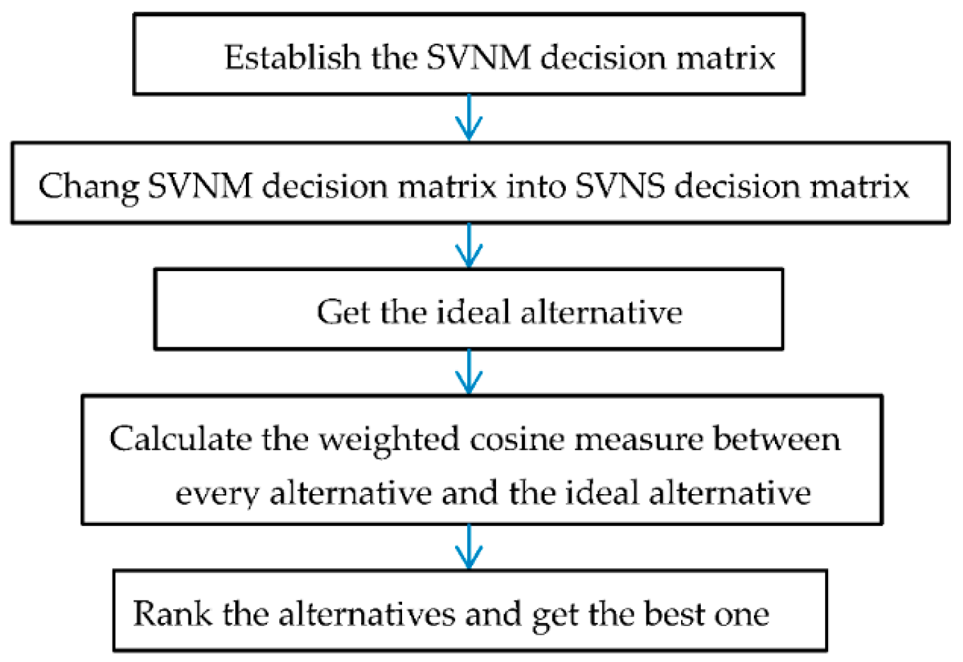
Step 1: By using Equation (7), we change the SVNM decision matrix D into SVNS decision matrix $\tilde{D}$, which is shown in

Table 2. The single-valued neutrosophic set (SVNS) decision matrix $\tilde{D}$.

	${\mathit{x}}_{\mathbf{1}}$	$\dots$
${\tilde{g}}_1$	$\langle x_1,1-{\displaystyle \prod _{k=1}^j}{\left(1-T_{g_{1}k}\left(x_1\right)\right)}^{p_{g_{1}k}},{\displaystyle \prod _{k=1}^j}{\left(I_{g_{1}k}\left(x_1\right)\right)}^{p_{g_{1}k}},{\displaystyle \prod _{k=1}^j}{\left(F_{g_{1}k}\left(x_1\right)\right)}^{p_{g_{1}k}}\rangle$	$\dots$
${\tilde{g}}_2$	$\langle x_1,1-{\displaystyle \prod _{k=1}^j}{\left(1-T_{g_{2}k}\left(x_1\right)\right)}^{p_{g_{2}k}},{\displaystyle \prod _{k=1}^j}{\left(I_{g_{2}k}\left(x_1\right)\right)}^{p_{g_{2}k}},{\displaystyle \prod _{k=1}^j}{\left(F_{g_{2}k}\left(x_1\right)\right)}^{p_{g_{2}k}}\rangle$	$\dots$
$\dots$	$\dots$	$\dots$
${\tilde{g}}_m$	$\langle x_1,1-{\displaystyle \prod _{k=1}^j}{\left(1-T_{g_{m}k}\left(x_1\right)\right)}^{p_{g_{m}k}},{\displaystyle \prod _{k=1}^j}{\left(I_{g_{m}k}\left(x_1\right)\right)}^{p_{g_{m}k}},{\displaystyle \prod _{k=1}^j}{\left(F_{g_{m}k}\left(x_1\right)\right)}^{p_{g_{m}k}}\rangle$	$\dots$
	${\mathit{x}}_{\mathit{n}}$
	$\langle x_n,1-{\displaystyle \prod _{k=1}^j}{\left(1-T_{g_{1}k}\left(x_n\right)\right)}^{p_{g_{1}k}},{\displaystyle \prod _{k=1}^j}{\left(I_{g_{1}k}\left(x_n\right)\right)}^{p_{g_{1}k}},{\displaystyle \prod _{k=1}^j}{\left(F_{g_{1}k}\left(x_n\right)\right)}^{p_{g_{1}k}}\rangle$
	$\langle x_n,1-{\displaystyle \prod _{k=1}^j}{\left(1-T_{g_{2}k}\left(x_n\right)\right)}^{p_{g_{2}k}},{\displaystyle \prod _{k=1}^j}{\left(I_{g_{2}k}\left(x_n\right)\right)}^{p_{g_{2}k}},{\displaystyle \prod _{k=1}^j}{\left(F_{g_{2}k}\left(x_n\right)\right)}^{p_{g_{2}k}}\rangle$
	$\dots$
	$\langle x_n,1-{\displaystyle \prod _{k=1}^j}{\left(1-T_{g_{m}k}\left(x_n\right)\right)}^{p_{g_{m}k}},{\displaystyle \prod _{k=1}^j}{\left(I_{g_{m}k}\left(x_n\right)\right)}^{p_{g_{m}k}},{\displaystyle \prod _{k=1}^j}{\left(F_{g_{m}k}\left(x_n\right)\right)}^{p_{g_{m}k}}\rangle$

.

Step 2: Setting $T_{g^{*}}\left(x_i\right)$ is the maximum truth value in each column $x_i\mathrm{of}\mathrm{the}\mathrm{decision}\mathrm{matrix}\tilde{D}$, $I_{g^{*}}\left(x_i\right)\mathrm{and}{F}_{g^{*}}\left(x_i\right)$ are the minimum indeterminate and falsity values in each column $x_i$ of the decision matrix $\tilde{D}$, respectively, the ideal solution can be determined as $x_i^{*}$.

$x_i^{*}=\langle T_{g^{*}}\left(x_i\right), I_{g^{*}}\left(x_i\right),F_{g^{*}}\left(x_i\right)\rangle$, for i = 1, 2, …, n.

So, we can get the ideal alternative $g^{*}=\{x_{1,}^{*},x_{2,}^{*},\dots ,x_n^{*}\}$.

Step 3: When the weight vector of attributes for the different importance of each attribute $x_i\left(i=1, 2,\dots ,n\right)$ is given by $w={\left(w_{1,}{w}_{2,}\dots ,w_n\right)}^T$ with $w_i\ge 0$ and ${\sum }_{i=1}^n{w}_i=1$, then we utilize the weighted cosine measure to deal with multiple attribute decision-making problems with SVNM information. The weighted cosine measure between an alternative ${\tilde{g}}_r\left(r=1, 2,\dots , m\right)$ and the ideal alternative $g^{*}$ can be calculated by using the following formula:

$$\begin{array}{ccc}\hfill {\rho }_w\left(g_r,g^{*}\right)& =& {\rho }_w\left({\tilde{g}}_r,g^{*}\right)\hfill \\ & & ={\displaystyle \sum _{i=1}^n}{w}_{i}cos\{\frac{\pi }{6}(\left|T_{{\tilde{g}}_r}\left(x_i\right)-T_{g^{*}}\left(x_i\right)\right|+\left|I_{{\tilde{g}}_r}\left(x_i\right)-I_{g^{*}}\left(x_i\right)\right|\hfill \\ & & +\left|F_{{\tilde{g}}_r}\left(x_i\right)-F_{g^{*}}\left(x_i\right)\right|)\}.\hfill \end{array}$$

(10)

Step 4: According to the values of ${\rho }_w\left({\tilde{g}}_r,g^{*}\right)$ for r = 1, 2, …, m, we rank the alternatives and select the best one.

Step 5: End.

The formalization of the steps is illustrated in Figure 1.

6. Numerical Example and Comparative Analysis

6.1. Numerical Example

Now, we utilize a practical example for the decision-making problem adapted from the literature [21] to demonstrate the applications of the proposed method under a SVNM environment. Now, one customer wants to buy a car, he selects four types of cars and evaluates them according to four attributes. Then, we build a decision model. There are four possible alternatives ($g_1,g_2,g_3,g_4)$ to be considered. The decision should be taken according to four attributes: fuel economy ($x_1),$ price ($x_2)$, comfort ($x_3),$ and safety ($x_4)$. The weight vector of these four attributes is given by $w={\left(0.5,0.25,0.125,0.125\right)}^T$. Then, the customer tests the four cars on the road with less obstacles and on the road with more obstacles, respectively, and after testing, some attributes may have two different evaluated values or the same value. So, the customer evaluates the four cars (alternatives) under the four attributes by the form of SVNMs.

Step 1: Establish the SVNM decision matrix D provided by the customer, which is given as the following SVNM decision matrix D in

Table 3. The SVNM decision matrix D.

	${\mathit{x}}_{\mathbf{1}}$	${\mathit{x}}_{\mathbf{2}}$	${\mathit{x}}_{\mathbf{3}}$	${\mathit{x}}_{\mathbf{4}}$
$g_1$	$\left(1,\langle 0.5,0.7,0.2\rangle \right),\left(1,\langle 0.7,0.3,0.6\rangle \right)$	$1,\langle 0.4,0.4,0.5\rangle$	$\left(1,\langle 0.7,0.7,0.5\rangle \right),\left(1,\langle 0.8,0.7,0.6\rangle \right)$	$\left(1,\langle 0.1,0.5,0.7\rangle \right),\left(1,\langle 0.5,0.2,0.8\rangle \right)$
$g_2$	$\left(1,\langle 0.9,0.7,0.5\rangle \right),\left(1,\langle 0.7,0.7,0.1\rangle \right)$	$1,\langle 0.7,0.6,0.8\rangle$	$2,\langle 0.9,0.4,0.6\rangle$	$(1,\langle 0.5,0.2,0.7\rangle ,\left(1,\langle 0.5,0.1,0.9\rangle \right)$
$g_3$	$(1,\langle 0.3,0.4,0.2\rangle ,\left(1,\langle 0.6,0.3,0.7\rangle \right)$	$1,\langle 0.2,0.2,0.2\rangle$	$(1,\langle 0.9,0.5,0.5\rangle ,\left(1,\langle 0.6,0.5,0.2\rangle \right)$	$(1,\langle 0.7,0.5,0.3\rangle ,\left(1,\langle 0.4,0.2,0.2\rangle \right)$
$g_4$	$(1,\langle 0.9,0.7,0.2\rangle ,\left(1,\langle 0.8,0.6,0.1\rangle \right)$	$1,\langle 0.3,0.5,0.2\rangle$	$(1,\langle 0.5,0.4,0.5\rangle ,\left(1,\langle 0.1,0.7,0.2\rangle \right)$	$2,\langle 0.4,0.2,0.8\rangle$

.

Step 2: By using Equation (7), we change the SVNM decision matrix D into SVNS decision matrix $\tilde{D}$, which is shown in

Table 4. The SVNS decision matrix $\tilde{D}$.

	${\mathit{x}}_{\mathbf{1}}$	${\mathit{x}}_{\mathbf{2}}$	${\mathit{x}}_{\mathbf{3}}$	${\mathit{x}}_{\mathbf{4}}$
${\tilde{g}}_1$	$\langle 0.85,0.21,0.12\rangle$	$\langle 0.4,0.4,0.5\rangle$	$\langle 0.94,0.49,0.3\rangle$	$\langle 0.55,0.1,0.56\rangle$
${\tilde{g}}_2$	$\langle 0.97,0.49,0.05\rangle$	$\langle 0.7,0.6,0.8\rangle$	$\langle 0.99,0.16,0.36\rangle$	$\langle 0.75,0.02,0.63\rangle$
${\tilde{g}}_3$	$\langle 0.72,0.12,0.14\rangle$	$\langle 0.2,0.2,0.2\rangle$	$\langle 0.96,0.25,0.1\rangle$	$\langle 0.82,0.1,0.06\rangle$
${\tilde{g}}_4$	$\langle 0.98,0.42,0.02\rangle$	$\langle 0.3,0.5,0.2\rangle$	$\langle 0.55,0.28,0.1\rangle$	$\langle 0.64,0.04,0.64\rangle$

.

Step 3: According to the decision matrix $\tilde{D}$, we can get the ideal alternative $g^{*}$:

$$g^{*}=\left\{\langle 0.98,0.12,0.02\rangle \langle 0.7,0.2,0.2\rangle \langle 0.99,0.16,0.1\rangle \langle 0.82,0.02,0.06\rangle \right\}.$$

(11)

Step 4: By applying the Equation (10), we can obtain the values of the weighted cosine measure between each alternative and the ideal alternative $g^{*}$ as follows:

$$\begin{array}{c}{\rho }_w\left(g_1,g^{*}\right)=0.9535,\hspace{1em}{\rho }_w\left(g_2,g^{*}\right)=0.9511,\hfill \\ \hfill {\rho }_w\left(g_3,g^{*}\right)=0.9813 \mathrm{and} {\rho }_w\left(g_4,g^{*}\right)=9616.\end{array}$$

(12)

Step 5: According to the above values of weighted cosine measure, we can rank the four alternatives: $g_3\succ g_4\succ g_1\succ g_2$. Therefore, the alternative $g_3$ is the best choice.

This example clearly indicates that the proposed decision-making method based on the weighted cosine measure of SVNMs is relatively simple and easy for dealing with multiple attribute decision-making problems under SVNM environment.

6.2. Comparative Analysis

In what follows, we compare the proposed method for SVNM with other existing related methods for SVNM; all the results are shown in

Table 5. The ranking orders by utilizing four different methods.

Method	Result	Ranking Order	The Best Alternative
Method 1 based on correlation coefficient in [11]	${\rho }_w\left(g_1,g^{*}\right)$ = 0.9053, ${\rho }_w\left(g_2,g^{*}\right)=$0.9017, ${\rho }_w\left(g_3,g^{*}\right)=$0.9516, ${\rho }_w\left(g_4,g^{*}\right)=$0.8816.	$g_3\succ g_1\succ g_2\succ g_4$	$g_3$
Method 2 based on similarity in [16]	${\rho }_w\left(g_1,g^{*}\right)$= 0.8204, ${\rho }_w\left(g_2,g^{*}\right)=$0.8108, ${\rho }_w\left(g_3,g^{*}\right)=$0.8867, ${\rho }_w\left(g_4,g^{*}\right)=$0.8358.	$g_3\succ g_4\succ g_2\succ g_1$	$g_3$
Method 3 based on similarity in [16]	${\rho }_w\left(g_1,g^{*}\right)$= 0.7898, ${\rho }_w\left(g_2,g^{*}\right)=$0.7121, ${\rho }_w\left(g_3,g^{*}\right)=$0.8125, ${\rho }_w\left(g_4,g^{*}\right)=$0.7553.	$g_3\succ g_1\succ g_4\succ g_2$	$g_3$
The proposed method	${\rho }_w\left(g_1,g^{*}\right)$= 0.9535, ${\rho }_w\left(g_2,g^{*}\right)=$0.9511, ${\rho }_w\left(g_3,g^{*}\right)=$0.9813, ${\rho }_w\left(g_4,g^{*}\right)=$9616.	$g_3\succ g_4\succ g_1\succ g_2$	$g_3$

.

From Table 5, these four methods have the same best alternative $g_3$. Many methods such as similarity measure, correlation coefficient, and cosine measure can all be used in SVNM to handle the multiple attribute decision-making problems and can get the similar results.

The proposed decision-making method can express and handle the multiplicity evaluated data given by decision makers or experts, while various existing neutrosophic decision-making methods cannot deal with these problems.

7. Conclusions

Based on the multiplicity evaluation in some real situations, this paper introduced a SVNM as a subclass of NM to express the multiplicity information and the operational relations of SVNMs. The SVNM is expressed by its one or more elements, which may have multiplicity. Therefore, SVNM has the desirable advantages and characteristics of expressing and handling the multiplicity problems, while existing neutrosophic sets cannot deal with them.

Then, we proposed the cosine measure of SVNMs and weighted cosine measure of SVNMs and investigated their properties. Based on the weighted cosine measure of SVNMs, the multiple attribute decision-making methods under SVNM environments was proposed, in which the evaluated values were taken the form of SVNMEs. Through the weighed cosine measure between each alternative and the ideal alternative, one can determine the ranking order of all alternatives and can select the best one. Finally, a practical example adapted from the literature [21] about buying cars was presented to demonstrate the effectiveness and practicality of the proposed method in this paper. According to the ranking orders, we can find that the ranking result with weighted cosine measures is agreement with the ranking results in literature [21]. Then, the proposed method is suitable for actual applications in multiple attribute decision-making problems with single-value neutrosophic multiplicity information.

In the future, we shall extend SVNMs to interval neutrosophic multisets and develop the application of interval neutrosophic multisets for handling the decision-making methods or other domains.

References

- Zadeh, L.A. Fuzzy sets. Inf. Control 1965, 8, 338–353. [Google Scholar] [CrossRef]
- Turksen, I.B. Interval valued fuzzy sets based on normal forms. Fuzzy Sets Syst. 1986, 20, 191–210. [Google Scholar] [CrossRef]
- Atanassov, K.T. Intuitionistic fuzzy sets. Fuzzy Sets Syst. 1986, 20, 87–96. [Google Scholar] [CrossRef]
- Smarandache, F. Neutrosophy: Neutrosophic Probability, Set, and Logic; American Research Press: Rehoboth, DE, USA, 1998. [Google Scholar]
- Wang, H.; Smarandache, F.; Zhang, Y.Q.; Sunderraman, R. Single Valued Neutrosophic Sets. Multispace MultiStruct. 2010, 4, 410–413. [Google Scholar]
- Wang, H.; Smarandache, F.; Zhang, Y.Q.; Sunderraman, R. Interval Neutrosophic Sets and Logic: Theory and Applications in Computing; Hexis: Phoenix, AZ, USA, 2005. [Google Scholar]
- Smarandache, F. n-Valued Refined Neutrosophic Logic and Its Applications in Physics. Prog. Phys. 2013, 4, 143–146. [Google Scholar]
- Ye, J.; Smarandache, F. Similarity Measure of Refined Single-Valued Neutrosophic Sets and Its Multicriteria Decision Making Method. Neutrosophic Sets Syst. 2016, 12, 41–44. [Google Scholar]
- Fan, C.X.; Ye, J. The Cosine Measure of Refined-Single Valued Neutrosophic Sets and Refined-Interval Neutrosophic Sets for Multiple Attribute Decision-Making. J. Intell. Fuzzy Syst. 2017, 33, 2281–2289. [Google Scholar] [CrossRef]
- Ye, J. Correlation Coefficient between Dynamic Single Valued Neutrosophic Multisets and Its Multiple Attribute Decision-Making Method. Information 2017, 8, 41. [Google Scholar] [CrossRef]
- Ye, J. Multicriteria decision-making method using the correlation coefficient under single-valued neutrosophic environment. Int. J. Gen. Syst. 2013, 42, 386–394. [Google Scholar] [CrossRef]
- Ye, J. A multicriteria decision-making method using aggregation operators for simplified neutrosophic sets. J. Intell. Fuzzy Syst. 2014, 26, 2459–2466. [Google Scholar]
- Broumi, S.; Smarandache, F. Several similarity measures of neutrosophic sets. Neutrosophic Sets Syst. 2013, 1, 54–62. [Google Scholar]
- Majumdar, P.; Samanta, S.K. On similarity and entropy of neutrosophic sets. J. Intell. Fuzzy Syst. 2014, 26, 1245–1252. [Google Scholar]
- Broumi, S.; Smarandache, F. Correlation coefficient of interval neutrosophic set. Appl. Mech. Mater. 2013, 436, 511–517. [Google Scholar] [CrossRef]
- Ye, J. Similarity measures between interval neutrosophic sets and their applications in multicriteria decision-making. J. Intell. Fuzzy Syst. 2014, 26, 165–172. [Google Scholar]
- Chi, P.P.; Liu, P.D. An extended TOPSIS method for the multiple attribute decision making problems based on interval neutrosophic set. Neutrosophic Sets Syst. 2013, 1, 63–70. [Google Scholar]
- Smarandache, F. Neutrosophic Perspectives: Triplets, Duplets, Multisets, Hybrid Operators, Modal Logic, Hedge Algebras and Applications; PonsEditions: Bruxelles, Brussels, 2017; pp. 115–123. [Google Scholar]
- Ye, S.; Ye, J. Dice Similarity Measure between Single Valued Neutrosophic Multisets and Its Application in Medical Diagnosis. Neutrosophic Sets Syst. 2014, 6, 48–53. [Google Scholar]
- Ye, J. Improved cosine similarity measures of simplified neutrosophic sets for medical diagnoses. Artif. Intell. Med. 2015, 63, 171–179. [Google Scholar] [CrossRef] [PubMed]
- Deli, I.; Ali, M.; Smarandache, F. Bipolar neutrosophic sets and their application based on multi-criteria decision making problems. In Proceedings of the International Conference on Advanced Mechatronic Systems, Beijing, China, 5 October 2015; pp. 249–254. [Google Scholar]
Figure 1.
Flowchart of the decision steps.