Network Embedding via a Bi-Mode and Deep Neural Network Model


College of System Engineering, National University of Defence Technology, Changsha 410073, China
*
Authors to whom correspondence should be addressed.
Symmetry 2018, 10(5), 180; https://doi.org/10.3390/sym10050180
Submission received: 6 April 2018
/
Revised: 10 May 2018
/
Accepted: 21 May 2018
/
Published: 22 May 2018
Abstract
:Network embedding (NE) is an important method to learn the representations of a network via a low-dimensional space. Conventional NE models focus on capturing the structural information and semantic information of vertices while neglecting such information for edges. In this work, we propose a novel NE model named BimoNet to capture both the structural and semantic information of edges. BimoNet is composed of two parts; i.e., the bi-mode embedding part and the deep neural network part. For the bi-mode embedding part, the first mode—named the add-mode—is used to express the entity-shared features of edges and the second mode—named the subtract-mode—is employed to represent the entity-specific features of edges. These features actually reflect the semantic information. For the deep neural network part, we firstly regard the edges in a network as nodes, and the vertices as links, which will not change the overall structure of the whole network. Then, we take the nodes’ adjacent matrix as the input of the deep neural network, as it can obtain similar representations for nodes with similar structure. Afterwards, by jointly optimizing the objective function of these two parts, BimoNet could preserve both the semantic and structural information of edges. In experiments, we evaluate BimoNet on three real-world datasets and the task of relation extraction, and BimoNet is demonstrated to outperform state-of-the-art baseline models consistently.
1. Introduction
Social and information networks are now ubiquitous, and contain rich and complex data that record the types and dynamics of human interactions. Thus, how to mine the information in networks is of high research and application value. Recently, network embedding (NE)—i.e., network representation learning (NRL)—has been proposed to represent the networks so as to realize network analysis, such as link prediction [1], clustering [2], and information retrieval [3]. NE aims to encode the information and features of each vertex into a low-dimensional space; i.e., learn real-valued vector representations for each vertex, so as to reconstruct the network in the learned embedding space. Compared with conventional symbol-based representations, NE could alleviate the issues of computation and sparsity, and thus manage and represent large-scale networks efficiently and effectively.
However, most existing NE models only focus on modeling vertices; for example, the classical NE model DeepWalk [4] utilizes random walks to capture the structure of the whole network and CANE [5] aims to leverage the semantic information of vertices. The edge is an important network component, and it is usually simplified as a binary or continuous value in those models. It is obvious that such simplification will waste the rich information contained in an edge. It is intuitive that, in real-world networks, edges also contain rich and variant meanings, as they encode the interactions between vertices, and their structure also influences the whole network. For example, many social media users are connected because of a common interest, and thus this interest could be a major component of the network, both semantically and structurally. Therefore, in this work, we propose a new NE model named BimoNet to make full use of both semantic and structural information of edges.
For semantic information, inspired by the recent work TransNet [6], which borrows the concept of relation extraction in Knowledge Graph (KG), we also utilize the triplets in KG to capture the features of relations. A fact (knowledge) in a knowledge graph is represented by a triplet (head_entity, relation, tail_entity), denoted as . We design a bi-mode embedding model to represent relations. The first mode is named the add-mode, where the relations are expressed by the shared features of entities (i.e., ). It is intuitive that a relation is an abstraction of the entity pairs having such a relation. Taking the relation Presidentof as an example, it should be the abstraction of all entity pairs like (Trump, America), (Putin, Russia), and (Xi Jinping, China). Thus, if we consolidate by summation and average all the features of the entity pairs, the features after consolidation could be used to express the features of relation Presidentof (rather than relations like CEOof). In general, for a triplet, the features of relation r is similar to the shared features of entity pair . The second mode is named the subtract-mode, where the relations are represented as a channel to offset the divergence and preserve the prominent individual features of head and tail entities (i.e., ). Such entity-specific features are not taken into consideration by add-mode, but are inherently possessed by entities. The motivation to integrate both modes of embedding is to model commonalities while allowing individual specificity. Although shared entity features by add-mode describe the intrinsic relationship between two entities, only using this could cause false positive entity pairs like (Trump, Russia), as they may have similar shared features. Therefore, we need to further distinguish the entity-specific features through subtract-mode embedding. To conclude, we use a bi-mode embedding to mine both the entity-shared features and entity-specific features of relations—that is, the semantic information of relations.
To represent structural information, for ease of understanding, we might as well regard relations as nodes and vertices as links, which will not change the overall structure of the network. Given a network, we can obtain a node’s adjacency matrix, where the entry of the matrix is greater than zero if and only if there exists a link between nodes. Thus, the adjacency matrix can represent the neighborhood structural information of each node; thus, by consolidating all the nodes’ adjacency matrix, we could capture the global structure of the network. Afterwards, we introduce a deep neural network autoencoder [7] and take the adjacency matrix as the input. A deep autoencoder can preserve the similarities between samples, thus making the nodes having similar neighborhood structure have similar latent representations.
There exist many symmetric and antisymmetric edges in a network, both semantically and structurally, so our model could handle the symmetry problem well simultaneously. We conducted experiments on three real-life network datasets constructed by TransNet. Experimental results show that BimoNet outperforms classical state-of-the-art NE models consistently. This demonstrates that our proposed model BimoNet’s power and efficiency in modeling relationships between vertices and edges, thus representing the whole network effectively.
The major contribution of the paper can be summarized into three components:
- We propose a novel network embedding model BimoNet, which describes relations’ semantic information by bi-mode embeddings and incorporates a deep neural network model to capture relations’ structural information;
- We are the first to fully mine both the semantic and structural information of edges in a network, which provides a new angle to represent the network; and
- The new model is evaluated and compared with existing models on real-life benchmark datasets and tasks, and experimental results on relation extraction verify that BimoNet outperforms state-of-the-art alternatives consistently.
The rest of the paper is structured as follows. We introduce the related work in Section 2, and then justify the intuitions of our method with its theoretical analysis in Section 3. Next, we conduct experimental studies on network relation extraction in Section 4. Finally, we conclude our findings in Section 5.
2. Related Work
2.1. Relation Extraction in Knowledge Graphs
Knowledge graphs (KGs) are typical large-scale multi-relational structures, which comprise a large amount of fact triplets, denoted as . Existing large-scale KGs such as Freebase [8], Wordnet [9], and YAGO [10] are all suffering from incompleteness. Thus, relation extraction is a crucial task in KG embedding work, with the goal of extracting relational facts between entities so as to complement the existing KGs. It usually performs as relation prediction, which is to predict whether a relation is suitable for a corrupted triplet .
Traditional KG embedding model RESCAL [11,12] is a relational latent feature model which represents triplets via pairwise interactions of latent features. MLPs [13] are also known as feed-forward neural networks, and in the context of multi-dimensional data they can be referred to a multi-way neural networks. This approach allows for considering alternative ways to represent triplets and use nonlinear functions to predict its existence. The SLM [14] model is proposed as a baseline of Neural Tensor Network (NTN), which is a simple nonlinear neural network model. An NTN [14] model is an extension of SLM model through considering the second-order relations into nonlinear neural networks.
However, models above all suffered from low efficiency as they all conducted the multiplication between entities and relations. Ref. [15] proposed an embedding model based on translation mechanism TransE, which interprets relations as translating operations between head and tail entities in the representation space (i.e., ). We could find that TransE is actually a variant of subtract-mode embedding, which suggests that our bi-mode embedding is compatible with TransE and further verifies our model’s ability in handling relationships between vertices and edges.
2.2. Deep Neural Networks
Representation learning has long been an essential problem of machine learning, and many works aim at learning representations for samples. Recently, deep neural network models have been proved as having powerful representation abilities, which can generate effective representations for various types of data. For example, in the image analysis field, Ref. [16] proposes a seven-layer convolutional neural network (CNN) to generate image representations for classification. Authors in [17] propose a multimodal deep model to learn image-text unified representations to achieve a cross-modality retrieval task.
However, fewer works have been done to learn network representation. Authors in [18] adopt restricted Boltzmann machines [19] to conduct collaborative filtering [20]. In [21], a heterogenous deep model is proposed to conduct heterogenous data embedding. NE embedding models TransNet [6] and SDNE [22] both use an autoencoder [7] to capture the label information of edges and the structural information of vertices, respectively. Our model BimoNet is different from those models, in that it aims to leverage the structural information of edges, which is a new angle to utilize in an autoencoder model.
2.3. Network Embedding
Our work solves the problem of network embedding, which aims to represent the networks through a low-dimensional space. Some earlier works, such as local linear embedding (LLE) [23] and IsoMAP [24], first construct the affinity graph based on the features vectors and obtain the network embedding by solving the leading eigenvectors as the network representations. More recently, DeepWalk [4] performs random walks over networks and introduces SkipGram [13]—an efficient word2vec embedding [13] method to learn the network embedding. LINE [25] optimizes the joint and conditional probabilities of edges in large-scale networks to learn vertex representations. Node2vec [26] proposes a biased random walks strategy to more efficiently explore the network structure. However, these models only encode the structural information into vertex embeddings. Furthermore, some works consider the incorporation of heterogenous information into network representation. Text-associated DeepWalk (TADW) [27] uses text information to improve the matrix factorization-based DeepWalk. Max-margin DeepWalk (MMDW) [28] utilizes the labeling information of vertices to learn discriminative network representations. Group-enhanced network embedding (GENE) [29] integrates existing group information into NE. Context-enhanced network embedding (CENE) [30] regards text content as a special kind of vertex , thus leveraging both structural and textual information in learning network embedding. In addition, SiNE [31] learns vertex representations in signed networks, in which each edge is either positive or negative. Nevertheless, it is worth noting that all of the models above over-simplify the edges and are not able to perfectly represent a network.
To the best of our knowledge, few works consider both the rich semantic information and structural information of edges, and extract and predict relations on edges in a detailed way. Therefore, we propose a novel model BimoNet to fill such research gaps.
3. Proposed Model
In this section, we propose a novel network embedding model BimoNet to integrate both the semantic and structural information of edges to learn the representation of networks.
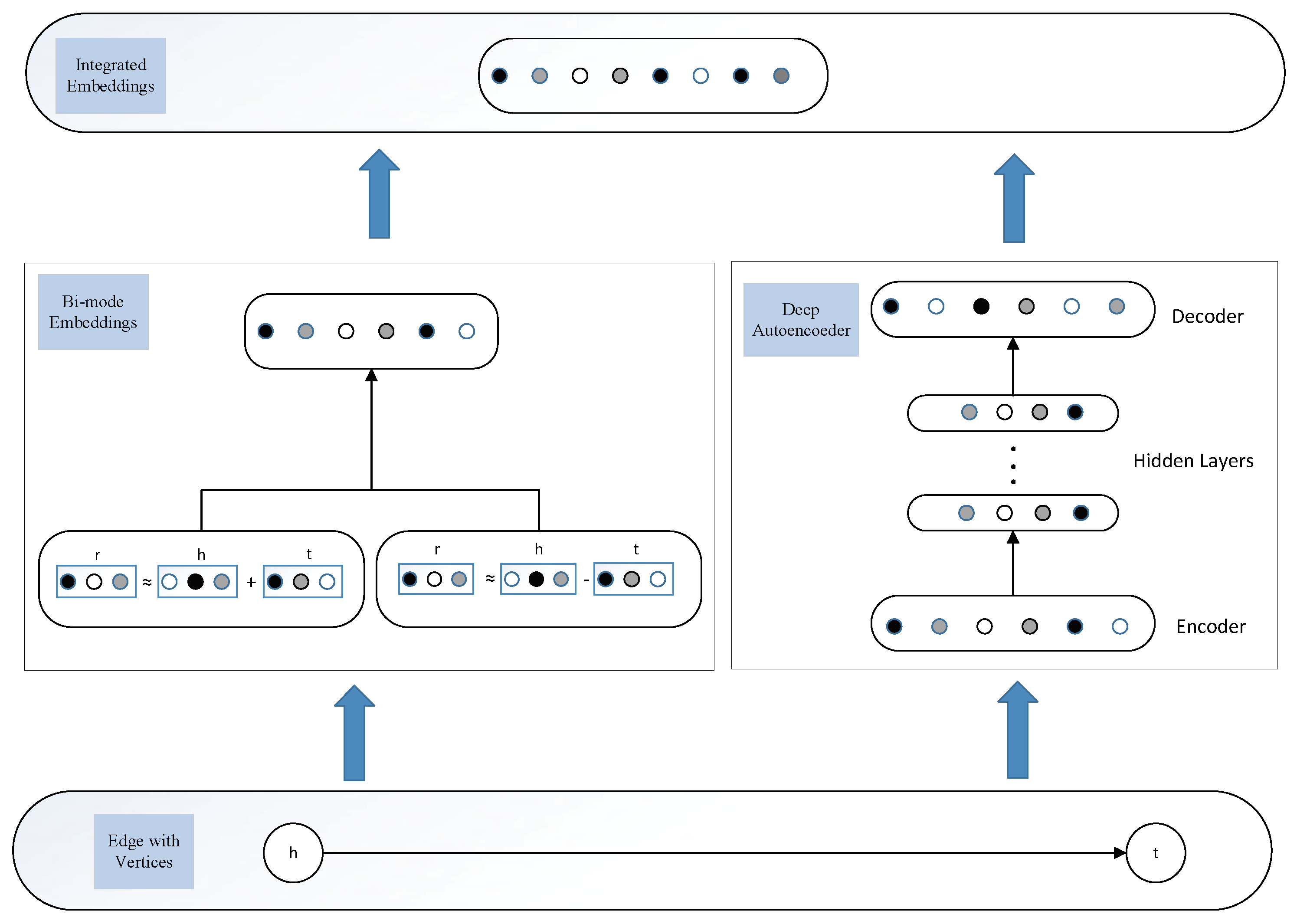
A sketch of the model framework is presented in Figure 1. From Figure 1, we could see that BimoNet is composed of two major components; i.e., the bi-mode embedding and deep autoencoder. In the following sections, we will first introduce the mechanism of bi-mode embedding in detail. After that, we will introduce how a deep antoencoder works to capture the structural information of edges. At last, we will present the integration of these two components to obtain the overall objective function of BimoNet.
3.1. Bi-Mode Embedding
Inspired by knowledge representation, which can extract relation features efficiently, we borrow concepts such as triplets in KG to help realize the bi-mode embedding. We will firstly introduce the common notations. A triplet is denoted as , where h denotes a head entity, r denotes a relation, and t denotes a tail entity, where head entities and tail entities are actually vertices in a network, and relations are actually edges. The bold letter , , represent the embeddings of . To discriminate the add-mode and subtract-mode, we denote their embeddings as , , and , , , respectively. The entity and relations take values in , where n is the dimension of entity and relation embeddings spaces. Next, we will introduce the detailed mechanism of add-mode and subtract-mode.
Add-Mode Embedding: The basic idea of add-mode embedding is that a relation is the abstraction of all the features of entity pairs. That is, some most common features will burst and individual features will correspondingly fade by consolidating all the features of entity pairs.
For each triplet , a head entity h and a tail entity t constitute an entity pair together, denoted as . Given an entity pair , there could be plenty of relations fitting the pair; on the other hand, one relation could also match a large number of entity pairs. Therefore, if we incorporate all the shared features of these entity pairs, this could be used to represent the unique features possessed by relation r, which is unlikely represented by other entity pairs without having relation r. That is, , mathematically.
Motivated by the above theory, we propose an add-mode embedding model that demonstrates that all the shared features of head entities and tail entities should be close to the features of relation r. In other words, when a triplet exists, it is expected that
From this, should be the closest relation of ; otherwise should be far away from . Moreover, under an energy-based framework, the energy of a triplet is equal to the distance between and , which could be measured by either or norms. Thus, the objective function can be represented as follows:
Subtract-Mode Embedding: Add-mode embedding can express the entity-shared features of relations, but neglects the entity-specific features. Recall the example that Trump is the president of America, and Putin is the president of Russia. Add-mode embedding could easily capture the representation features between Trump (resp. Putin) and America (resp. Russia). Nevertheless, if we intentionally pair Trump with Russia, add-mode embedding may falsely figure that the corrupted entity pair as correct, as the shared features between Trump and Russia may be fairly close to the features of relation Presidentof. We attribute this to the fact that add-mode embedding only focuses on shared features while it underestimates the significance of the individual features of entities.
To cover the shortage of add-mode embedding, we further adopt the subtract-mode embedding so as to capture the entity-specific features. For a triplet , the embedding of relation r describes the discrepancies between h and t by calculating the differences between their embeddings. That is, , mathematically. In this case, it is expected that is close to , meanwhile it is far away from other entities. Similarly, the objective function can be represented as follows:
Consequently, we can obtain the overall objective function of bi-mode embedding via integrating the two complementary methods together:
To learn such embeddings, for each triplet and its corrupted sample , we minimize the following margin-based ranking loss function over the training set,
where is a margin hyperparameter and the loss function above encourages the discrimination between positive triplets and corrupted triplets. is a negative sample that is obtained by randomly replacing the original head or tail entity (resp. relation) with another disconnected entity (resp. relation).
3.2. Deep Autoencoder
Here, we introduce the detailed mechanism of a deep autoencoder to illustrate its ability to capture the structural information of edges. Firstly, for ease of understanding, we propose a bold concept in that we regard edges as nodes and vertices as links to build a new network. However, such changes will not influence the overall structure of the original network, so we see this concept as quite acceptable.
Given a modified network , where N denotes the nodes that are actually edges and L denotes the links that are actually vertices, we can obtain its adjacency matrix of nodes. S contains m instances denoted as . For each instance , if and only if node and node have a connected link. Hence, expresses the neighborhood structure of the node and S encodes the neighborhood structure of each node, thus obtaining the global structure of the network. Next, we introduce how we incorporate the adjacency matrix into the traditional deep autoencoder [7].
The deep autoencoder comprises two parts—i.e., the encoder part and the decoder part. The encoder consists of multiple nonlinear functions mapping the input data to the representation space. The decoder also consists of multiple nonlinear functions that map the representations from representation space to reconstruction space. Given the input , the hidden representations for each layer are presented as follows:
denotes the activation function and we apply the sigmoid function in this paper. After obtaining , we can correspondingly obtain the output by reversing the calculation process of the encoder. The autoencoder aims to minimize the reconstruction error of the output and the input. The loss function is shown as follows:
Authors in [7] proved that although minimizing the reconstruction loss does not explicitly preserve the similarity between samples, its reconstruction criterion can smoothly capture the data manifolds, thus preserving the similarity between samples. Therefore, considering our case wherein we use the adjacency matrix as the input to the autoencoder (i.e., ), since encodes the neighborhood structure of node , the reconstruction calculation will make the nodes that have similar neighborhood structure have similar representations as well.
However, we cannot directly apply this reconstruction function to our problem due to the sparsity of the input matrix. That is, the number of zero elements in is much larger than that of non-zero elements, which means that the autoencoder tends to reconstruct the zero elements instead of non-zero ones. This is not what we expect. Hence, we impose more penalty to the reconstruction error of the non-zero element than that of zero elements. The modified objective function is shown as follows:
where ⊙ denotes the Hadamard dot, i.e., element-wise multiplication, . If , ; otherwise, , where is the hyperparameter to balance the weight of non-zero elements in autoencoder. Now, by utilizing the modified deep autoencoder with the input adjacency matrix , the nodes that have similar structures will be mapped closely in the representation space, which is guaranteed by the reconstruction criterion. Namely, a deep autoencoder could capture the structural information of the network by the reconstructing process on nodes (in our case, edges).
3.3. The Integrated Model
Here, we integrate the bi-mode embedding and the deep autoencoder representation into a unified network embedding model named BimoNet, which preserves the ability to model both semantic and structural information. To maintain the consistency of the two objective functions, we take the norm in bi-mode embedding as the norm. Consequently, we obtain the overall objective function as follows:
where and are hyperparameters that control the weights of the autoencoder objective function and the regulation function, respectively. Additionally, we take the regularizer , which could prevent overfitting as the norm, shown as follows:
4. Experiments and Analysis
We empirically evaluate our model and related baseline models by conducting the experimental relation extraction on three real-world datasets. Relation extraction usually performs as relation prediction, which is to predict whether a relation fits a specific entity pair. We first introduce the data sets in the first place, then introduce other baseline algorithms, along with the evaluation metrics and parameter settings of all models, and finally analyze the experimental results.
4.1. Datasets
We chose the datasets from ArnetMiner [34], which were constructed by TransNet [6], in order to compare our model with this recent state-of-the-art model along with the conventional models. ArnetMiner is an online academic website that provides a search and mining service for researcher social networks. It releases a large-scale co-author network [35], which consists of 1,712,433 authors, 2,092,356 papers, and 4,258,615 collaboration relations. In this network, authors collaborate with different people in different research fields, and the co-authored papers can reflect the relations with them in detail. Therefore, TransNet constructed the co-authored network with edges representing their shared research topics. For example, author A and author B are co-authors, so their shared features are likely to reflect their shared research topics, and this could be realized via add-mode embedding. However, author A and author B are two different researchers, so we apply the subtract-mode embedding to maintain their individual, i.e., entity-specific features. In addition, an author who is the leader of a research group tends to collaborate with many other researchers, whereas some authors may only have a few co-authors. Such phenomenon illustrates the structure of the ArnetMiner network and we capture such information via the deep autoencoder mechanism. Notice that, as the edges in this co-author network are undirected, the constructed datasets replace each edge with two directed edges having opposite directions.
To better study the characteristics of different models, the datasets are constructed with three different scales—i.e., Arnet-S (small), Arnet-M (medium), and Arnet-L (large). Table 1 illustrates the detailed statistics of these three datasets.
4.2. Baseline Algorithms
We introduce the following network embedding models as baselines.
DeepWalk [4] employs random walks to generate random walk sequences over networks. With these sequences, it adopts SkipGram [13]—an efficient word representation model—to learn vertices embeddings.
LINE [25] defines objective functions to preserve the first-order or second-order proximity separately. After optimizing the objective functions, it concatenates these representations in large-scale networks.
node2vec [26] proposes a biased random walk algorithm based on DeepWalk to explore the neighborhood structure more efficiently.
TransNet [6] borrows the concept of the translation mechanism from the conventional knowledge embedding method TransE [15] to capture the semantic information of edges. Then, it employs a deep neural network to further mine the label information of edges, which is still an aspect of the semantic information.
In addition, we also compare our model with TransE, as our training triplets are actually identical to that in a knowledge graph. Hence, our datasets could be directly employed to train TransE and adopt the similarity-based predicting method as presented in [15].
4.3. Experimental Setup
Relation extraction is used to predict the missing relations in a positive triplet . In this task, we randomly replace the missing relations by the existing relations in a knowledge graph, and rank these relations in descending order via the objective function. Instead of finding one best relation, this task stores the rank of the correct relation. After doing this, we have two evaluation metrics based on the rank we get for the correct relation. One is the MeanRank, which is the mean of predicted ranks of all relations. The other one is the proportion of all correct relations ranked in top k, denoted as hits@k. We chose hits@1, hits@5 and hits@10 in this metric. Obviously, a lower MeanRank and a higher hits@k represent a better performance for a specific model. When dealing with the corrupted triplets, we should note that, though replacing the relations, a triplet may also exist in a knowledge graph as positive, so it is reasonable to remove those corrupted triplets from the negative triplets set. We call the original evaluation setting as “Raw”, and the setting filtering the corrupted triplets that appear in either training, validation, or test sets before ranking as “Filter” [15]. The test and validation datasets are randomly selected with their amounts illustrated in Table 1, while the remaining data are selected to be the training datasets. We first train the training datasets to obtain the embeddings of the network and tune the parameters via the output from validation datasets; afterwards, we use the optimized embeddings learned from both training and validation datasets as the input to the test datasets, so as to obtain the final experimental results.
We selected the dimension n of the entities and relations embeddings among {50, 100, 150, 200, 300}, the regularization parameter among {0.1, 0.03, 0.01, 0.003, 0.001, 0.0003, 0.0}, the initial learning rate of Adam among {0.05, 0.02, 0.01, 0.001, 0.0003}, the hyperparameter which controls the weight of autoencoder loss among {5, 1, 0.5, 0.05, 0.005}, and the hyperparameter which balances the weight of non-zero elements in autoencoder among {10, 20, 30, 60, 80 ,100}. Additionally, we set the margin as 1. As for the size m of the input to the autoencoder, it would be too large if we take every edge into account and cause sparsity issues. Instead, we set m to be around of the total number of edges in each dataset, which is still able to reflect the structure of the network. As illustrated in Section 3.2, edges sharing similar structure will correspondingly have similar outputs from the autoencoder, thus expressing the structural information of the network. In order to balance the expressiveness and complexity of the deep autoencoder model, we set the hidden layers as two for all datasets. For Arnet-S, the best configuration obtained by the valid set is: , , , , , and . For Arnet-M, the best configuration is: , , , , , and . For Arnet-L, the best configuration is: , , , , , and . Moreover, we set the training iteration of our experiments to be 100. As for the other baselines, their configurations are directly adopted from TransNet [6], for TransNet has conducted the parameter optimization for these baselines. Moreover, we also conduct experiments on the model with only bi-mode embedding and only autoencoder, denoted as BimoNet-Bi and BimoNet-Net, respectively.
All the experiments are conducted on tensorflow with version 0.12.0, implemented by Python 2.7. In addition, we train all models on a one-core GPU GTX-1080.
4.4. Experimental Results and Analysis
Experimental results for the three datasets are presented in Table 2, Table 3 and Table 4. In these tables, the left four matrices are raw results, and the right four are filtered ones. As introduced above, a higher and a lower represent a better performance for a specific model. From these tables, we can observe that BimoNet outperformed other baseline models consistently on all datasets in both Filter and Raw settings on every metric. To be more specific, BimoNet even outperformed the best baseline (i.e., TransNet), by about to absolutely on all metrics and . This illustrates the robustness and effectiveness of BimoNet in modeling and predicting relations between vertices.
All traditional network embedding models DeepWalk, LINE and node2vec performed poorly in the relation extraction task under various situations, not even half better than BimoNet on every metric, which is attributed to the neglect of semantic and structural information of edges when learning the network representations. Those embedding models only focused on capturing the structural information of nodes in a network. As for TransE, TransNet, and BimoNet, they all incorporate the semantic information of edges into the learned representations, thus obtaining relatively decent results. This demonstrates that the semantic information of edges plays an essential part in network embedding, and further proves our bi-mode embedding model’s ability to capture such information. Nonetheless, compared to BimoNet, TransE and TransNet still have poor performances on every metric, due to their limitation of only focusing on the semantic information while underestimating the structural information of edges. Similarly, this indicates the importance of structural information and the rationality of the deep autocoder in exploring such information. Furthermore, BimoNet outperforms BimoNet-Bi and BimoNet-Net significantly, which further illustrates that it is insufficient to utilize only one kind of information. To conclude, BimoNet leverages both the semantic information and structural information of edges in order to learn the network representations as completely as possible.
In addition, BimoNet performed stably on networks of different scales. Specifically, on filtered hit@10, its performance only had a small decrease from to , despite the fact that datasets became much larger. However, other NE models suffered from a much more significant drop than BimoNet as the network grew larger. This demonstrates the stability and flexibility of BimoNet, which could be applied to efficiently model the large-scale real-life networks.
To analyze the efficiency of our model, Table 5 illustrates the running time of every model. We can observe that DeepWalk, LINE and node2vec cost relatively less time as they only capture the structure of a network and suffer from poor performance. BimoNet cost the most time with around 10 % more than TransNet due to the complexity of its mechanism. However, considering the improvements achieved by BimoNet illustrated above, we find such cost of time quite acceptable.
4.5. Relation Comparison
To further investigate the power of BimoNet in representing relations between vertices, we compared BimoNet with TransNet under high-frequency relations and low-frequency relations. We experiment with the top 5 relations and bottom 5 relations on Arnet-S, and the filtered and results are presented in Table 6.
From this, we observe that BimoNet outperformed TransNet consistently in both types of relations. We attribute this to the fact that relations having a similar frequency tend to have similar structures. In other words, relation frequency reflects its structure, to some extent. Therefore, through the use of the deep autoencoder that can explore the structural information of edges, BimoNet improves its prediction on relations regardless of their frequency.
4.6. Parameter Sensitivity
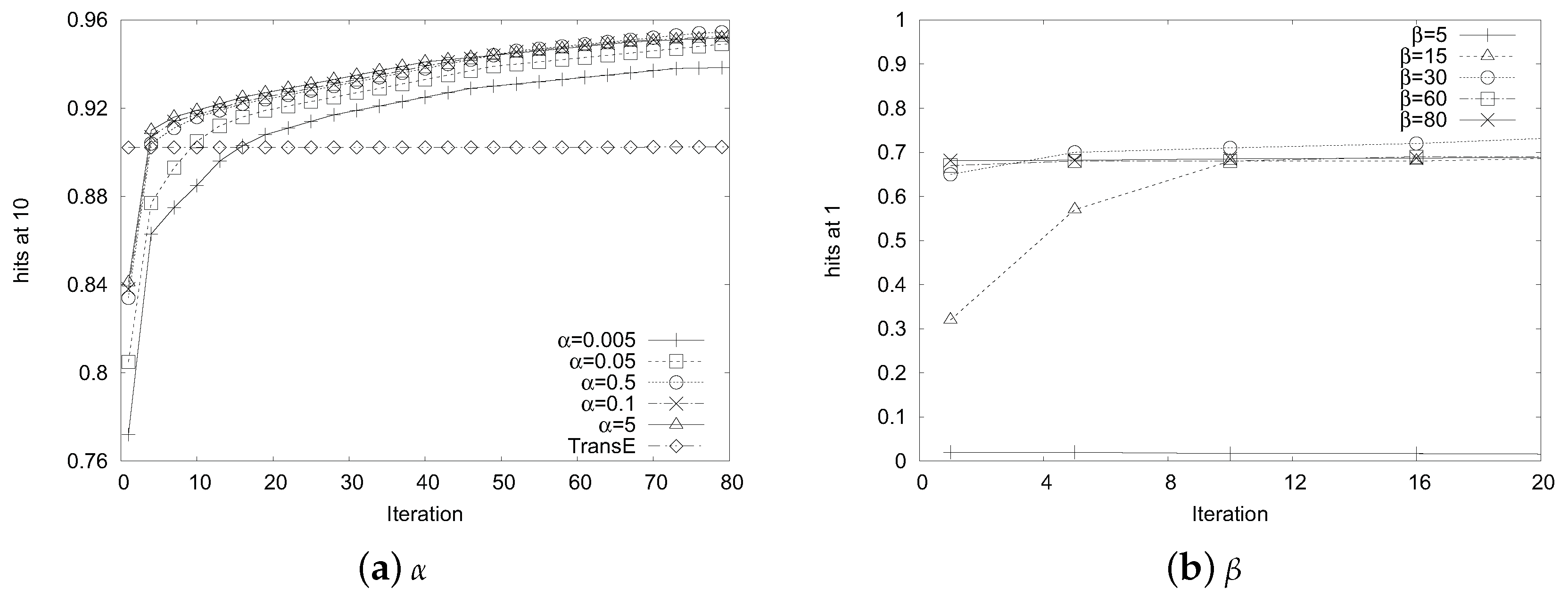
We investigate the parameter sensitivity in this section. To be specific, we evaluate two crucial hyperparameters (i.e., and ), which is crucial to experimental results, and experiment on Arnet-S.
In order to find a good balanced point between bi-mode embedding and deep autocoder, we show how the value affects the performance in Figure 2a. The parameter balances the weight of auto- encoder loss and bi-mode embedding loss. We chose the filtered hits@10 metric for comparison. From Figure 2a, we observe that the performance of BimoNet improved rapidly at the beginning, and then became stable. Although varied a lot, all of BimoNet’s performances exceeded that of TransE at around 20 iterations. This demonstrates that BimoNet is insensitive to , so it can be easily implemented and well trained in practice.
As for , it balances the reconstruction weight of the none-zero elements in autoencoder. The larger the , the more prone the model will be to reconstruct the non-zero elements. The filtered results in the validation set under different values of are presented in Figure 2b. From this, we observe that the performance becomes stable as iteration grows. When , the autoencoder puts too much weight on zero elements, thus performing rather poorly. Similarly, BimoNet is also not so sensitive to , which further illustrates its feasibility to real-world networks.
4.7. Discussion
We applied our model on a subset of ArnetMiner to conduct the experiment relation prediction, and the results have proved BimoNet’ ability of representing this network. The reason that BimoNet outperforms TransNet and TransE is that it leverages the auto-encoder to capture the structure information of the edge, while the other two only focus on the semantic information. Our efficiency is sacrificed since BimoNet has larger complexity; however, it is acceptable as it has improved the performance a lot.
In addition, we also discuss the potential applications of BimoNet on ArnetMiner or even more real-life networks. For example, on ArnetMiner, if an author wants to reach out for a research group to collaborate or explore a research field further, relation prediction could help select authors or even group leaders who are strongly related to this research field via the ranking list. Therefore, relation prediction realized by BimoNet could be equipped to a recommend system. For instance, in a social media network like Twitter, such system could help recommend users who share similar interests or similar friends. An online-shopping website could recommend you with objects that you may be interested via their relations between the objects you have purchased.
5. Conclusions
In this paper, we introduce the model BimoNet, which embeds a network in low-dimensional vector space. BimoNet mainly has two parts: the bi-mode embedding part and the deep neural network part. For the bi-mode embedding part, we used the add-mode to explore the entity-shared features of edges and the subtract-mode to represent the entity-specific features of edges. For the deep neural network, we regard the edges in a network as nodes and the vertices as links in the first place. Then, we take the nodes’ adjacent matrix as the input of the deep neural network and it can obtain similar representations for nodes having similar structure. After that, by jointly optimizing the objective function of these two parts, BimoNet could capture both the semantic and structural information of edges. Experimental results on relation extraction verified BimoNet’s ability to model the edges between vertices, as it outperformed baseline models consistently.
As future work, we plan to further explore at least the following two directions:
- We intend to integrate the semantic and structural information of edges with that of vertices, in order to further mine the network information and obtain an even more powerful network embedding model; and
- Existing network embedding models do not consider the new vertices and edges while networks in the real world are becoming larger and larger, so it is crucial to find a way to represent these new vertices and edges.
Author Contributions
Y.F. and X.Z. conceived and designed the experiments; Y.F. performed the experiments; Z.T. and W.X. analyzed the data; Y.F. and Z.T. wrote the paper.
Funding
This research was funded by National Nature Science Foundation of China (NSFC) grant numbers 71690233 and 71331008.
Conflicts of Interest
The authors declare no conflict of interest.
References
- Liben-Nowell, D.; Kleinberg, J.M. The link prediction problem for social networks. In Proceedings of the 2003 ACM CIKM International Conference on Information and Knowledge Management, New Orleans, LA, USA, 2–8 November 2003; pp. 556–559. [Google Scholar]
- Shepitsen, A.; Gemmell, J.; Mobasher, B.; Burke, R.D. Personalized recommendation in social tagging systems using hierarchical clustering. In Proceedings of the 2008 ACM Conference on Recommender Systems (RecSys 2008), Lausanne, Switzerland, 23–25 October 2008; pp. 259–266. [Google Scholar]
- Weiss, Y.; Torralba, A.; Fergus, R. Spectral Hashing. In Proceedings of the Twenty-Second Annual Conference on Neural Information Processing Systems, Vancouver, BC, Canada, 8–11 December 2008; pp. 1753–1760. [Google Scholar]
- Perozzi, B.; Al-Rfou, R.; Skiena, S. DeepWalk: Online learning of social representations. In Proceedings of the 20th ACM SIGKDD International Conference on Knowledge Discovery and Data Mining (KDD’14), New York, NY, USA, 24–27 August 2014; pp. 701–710. [Google Scholar]
- Tu, C.; Liu, H.; Liu, Z.; Sun, M. CANE: Context-Aware Network Embedding for Relation Modeling. In Proceedings of the 55th Annual Meeting of the Association for Computational Linguistics (ACL), Vancouver, BC, Canada, 30 July–4 August 2017; Volume 1, pp. 1722–1731. [Google Scholar]
- Tu, C.; Zhang, Z.; Liu, Z.; Sun, M. TransNet: Translation-Based Network Representation Learning for Thuscial Relation Extraction. In Proceedings of the International Joint Conference on Artificial Intelligence (IJCAI), Melbourne, Australia, 19–25 August 2017; pp. 2864–2870. [Google Scholar]
- Salakhutdinov, R.; Hinton, G.E. Semantic hashing. Int. J. Approx. Reason. 2009, 50, 969–978. [Google Scholar] [CrossRef]
- Bollacker, K.D.; Evans, C.; Paritosh, P.; Sturge, T.; Taylor, J. Freebase: A collaboratively created graph database for structuring human knowledge. In Proceedings of the ACM SIGMOD International Conference on Management of Data (SIGMOD 2008), Vancouver, BC, Canada, 10–12 June 2008; pp. 1247–1250. [Google Scholar]
- Miller, G.A. WordNet: A Lexical Database for English. Commun. ACM 1995, 38, 39–41. [Google Scholar] [CrossRef]
- Suchanek, F.M.; Kasneci, G.; Weikum, G. Yago: A core of semantic knowledge. In Proceedings of the 16th International Conference on World Wide Web (WWW 2007), Banff, AB, Canada, 8–12 May 2007; pp. 697–706. [Google Scholar]
- Nickel, M.; Tresp, V.; Kriegel, H. A Three-Way Model for Collective Learning on Multi-Relational Data. In Proceedings of the 28th International Conference on Machine Learning (ICML 2011), Bellevue, WA, USA, 28 June–2 July 2011; pp. 809–816. [Google Scholar]
- Nickel, M.; Tresp, V.; Kriegel, H. Factorizing YAGO: scalable machine learning for linked data. In Proceedings of the 21st World Wide Web Conference 2012 (WWW 2012), Lyon, France, 16–22 April 2012; pp. 271–280. [Google Scholar]
- Mikolov, T.; Chen, K.; Corrado, G.; Dean, J. Efficient Estimation of Word Representations in Vector Space. arXiv, 2013; arXiv:1301.3781. [Google Scholar]
- Socher, R.; Chen, D.; Manning, C.D.; Ng, A.Y. Reasoning With Neural Tensor Networks for Knowledge Base Completion. In Proceedings of the 27th Annual Conference on Neural Information Processing Systems 2013, Lake Tahoe, NE, USA, 5–10 December 2013; pp. 926–934. [Google Scholar]
- Bordes, A.; Usunier, N.; García-Durán, A.; Weston, J.; Yakhnenko, O. Translating Embeddings for Modeling Multi-relational Data. In Proceedings of the 27th Annual Conference on Neural Information Processing Systems 2013, Lake Tahoe, NE, USA, 5–10 December 2013; pp. 2787–2795. [Google Scholar]
- Krizhevsky, A.; Sutskever, I.; Hinton, G.E. ImageNet classification with deep convolutional neural networks. Commun. ACM 2017, 60, 84–90. [Google Scholar] [CrossRef]
- Wang, D.; Cui, P.; Ou, M.; Zhu, W. Deep Multimodal Hashing with Orthogonal Regularization. In Proceedings of the 24th International Conference on Artificial Intelligence (IJCAI’15), Buenos Aires, Argentina, 25–31 July 2015; pp. 2291–2297. [Google Scholar]
- Georgiev, K.; Nakov, P. A non-IID Framework for Collaborative Filtering with Restricted Boltzmann Machines. In Proceedings of the 30th International Conference on International Conference on Machine Learning (ICML’13), Atlanta, GA, USA, 16–21 June 2013; Volume 28, pp. 1148–1156. [Google Scholar]
- Hinton, G.E. Training Products of Experts by Minimizing Contrastive Divergence. Neural Comput. 2002, 14, 1771–1800. [Google Scholar] [CrossRef] [PubMed]
- Salakhutdinov, R.; Mnih, A.; Hinton, G.E. Restricted Boltzmann machines for collaborative filtering. In Proceedings of the 24th International Conference on Machine Learning, (ICML 2007), Corvallis, OR, USA, 20–24 June 2007; pp. 791–798. [Google Scholar]
- Chang, S.; Han, W.; Tang, J.; Qi, G.; Aggarwal, C.C.; Huang, T.S. Heterogeneous Network Embedding via Deep Architectures. In Proceedings of the 21th ACM SIGKDD International Conference on Knowledge Discovery and Data Mining, Sydney, Australia, 10–13 August 2015; pp. 119–128. [Google Scholar]
- Wang, D.; Cui, P.; Zhu, W. Structural Deep Network Embedding. In Proceedings of the 22nd ACM SIGKDD International Conference on Knowledge Discovery and Data Mining, San Francisco, CA, USA, 13–17 August 2016; pp. 1225–1234. [Google Scholar]
- Roweis, S.T.; Saul, L.K. Nonlinear Dimensionality Reduction by Locally Linear Embedding. Science 2000, 290, 2323–2326. [Google Scholar] [CrossRef] [PubMed]
- Tenenbaum, J.B.; Silva, V.D.; Langford, J.C. A Global Geometric Framework for Nonlinear Dimensionality Reduction. Science 2000, 290, 2319–2323. [Google Scholar] [CrossRef] [PubMed]
- Tang, J.; Qu, M.; Wang, M.; Zhang, M.; Yan, J.; Mei, Q. LINE: Large-scale Information Network Embedding. In Proceedings of the 24th International Conference on World Wide Web (WWW 2015), Florence, Italy, 18–22 May 2015; pp. 1067–1077. [Google Scholar]
- Grover, A.; Leskovec, J. node2vec: Scalable Feature Learning for Networks. In Proceedings of the 22nd ACM SIGKDD International Conference on Knowledge Discovery and Data Mining, San Francisco, CA, USA, 13–17 August 2016; pp. 855–864. [Google Scholar]
- Yang, C.; Liu, Z.; Zhao, D.; Sun, M.; Chang, E.Y. Network Representation Learning with Rich Text Information. In Proceedings of the 24th International Conference on Artificial Intelligence (IJCAI’15), Buenos Aires, Argentina, 25–31 July 2015; pp. 2111–2117. [Google Scholar]
- Tu, C.; Zhang, W.; Liu, Z.; Sun, M. Max-Margin DeepWalk: Discriminative Learning of Network Representation. In Proceedings of the Twenty-Fifth International Joint Conference on Artificial Intelligence (IJCAI’16 ), New York, NY, USA, 9–15 July 2016; pp. 3889–3895. [Google Scholar]
- Chen, J.; Zhang, Q.; Huang, X. Incorporate Group Information to Enhance Network Embedding. In Proceedings of the 25th ACM International on Conference on Information and Knowledge Management (CIKM ’16), Indianapolis, IN, USA, 24–28 October 2016; pp. 1901–1904. [Google Scholar]
- Sun, X.; Guo, J.; Ding, X.; Liu, T. A General Framework for Content-enhanced Network Representation Learning. arXiv, 2016; arXiv:1610.02906. [Google Scholar]
- Wang, S.; Tang, J.; Aggarwal, C.C.; Chang, Y.; Liu, H. Signed Network Embedding in Social Media. In Proceedings of the 2017 SIAM International Conference on Data Mining (SDM), Houston, TX, USA, 27–29 April 2017; pp. 327–335. [Google Scholar]
- Srivastava, N.; Hinton, G.E.; Krizhevsky, A.; Sutskever, I.; Salakhutdinov, R. Dropout: A simple way to prevent neural networks from overfitting. J. Mach. Learn. Res. 2014, 15, 1929–1958. [Google Scholar]
- Kingma, D.P.; Ba, J. Adam: A Method for Stochastic Optimization. arXiv, 2014; arXiv:1412.6980. [Google Scholar]
- Tang, J.; Zhang, J.; Yao, L.; Li, J.; Zhang, L.; Su, Z. ArnetMiner: Extraction and mining of academic social networks. In Proceedings of the 14th ACM SIGKDD International Conference on Knowledge Discovery and Data Mining, Las Vegas, NE, USA, 24–27 August 2008; pp. 990–998. [Google Scholar]
- Available online: https://github.com/thunlp/TransNet/blob/master/data.zip (accessed on 13 January 2018).
Figure 1.
Model framework of BimoNet.

Figure 2.
Parameter sensitivity.


Table 1.
Dataset statistics.
| Datasets | Arnet-S | Arnet-M | Arnet-L |
|---|---|---|---|
| Vertices | 187,939 | 268,037 | 945,589 |
| Edges | 1,619,278 | 2,747,386 | 5,056,050 |
| Train | 1,579,278 | 2,147,386 | 3,856,050 |
| Test | 20,000 | 300,000 | 600,000 |
| Valid | 20,000 | 300,000 | 600,000 |
Table 2.
Relation extraction results on Arnet-S with Metrics hits@k and MeanRank.
| Metric | hits@1 | hits@5 | hits@10 | MeanRank | hits@1 | hits@5 | hits@10 | MeanRank |
|---|---|---|---|---|---|---|---|---|
| DeepWalk | 13.55 | 37.26 | 50.34 | 19.78 | 18.48 | 39.57 | 52.72 | 19.02 |
| LINE | 11.25 | 31.56 | 44.37 | 23.22 | 15.35 | 33.69 | 45.88 | 22.21 |
| node2vec | 13.62 | 36.55 | 50.31 | 19.35 | 18.13 | 39.31 | 52.34 | 19.13 |
| TransNet | 47.78 | 86.87 | 92.13 | 5.12 | 77.18 | 90.34 | 93.67 | 3.98 |
| TransE | 39.17 | 78.32 | 88.73 | 5.33 | 57.58 | 84.12 | 90.01 | 4.51 |
| BimoNet | 51.34 | 89.69 | 95.12 | 4.42 | 81.34 | 93.55 | 95.56 | 3.22 |
| BimoNet-Bi | 44.34 | 83.42 | 89.45 | 5.89 | 73.23 | 85.42 | 87.32 | 6.23 |
| BimoNet-Net | 20.14 | 40.58 | 60.49 | 15.34 | 40.32 | 68.35 | 70.51 | 14.59 |
Table 3.
Relation extraction results on Arnet-M with Metrics hits@k and MeanRank.
| Metric | hits@1 | hits@5 | hits@10 | MeanRank | hits@1 | hits@5 | hits@10 | MeanRank |
|---|---|---|---|---|---|---|---|---|
| DeepWalk | 7.39 | 21.34 | 29.32 | 82.19 | 11.33 | 23.11 | 30.98 | 78.14 |
| LINE | 5.78 | 17.21 | 24.83 | 95.39 | 8.68 | 19.02 | 26.23 | 92.15 |
| node2vec | 7.34 | 21.06 | 29.55 | 80.54 | 11.45 | 23.41 | 31.37 | 78.27 |
| TransNet | 27.82 | 66.47 | 76.12 | 25.35 | 58.35 | 74.71 | 79.72 | 22.71 |
| TransE | 19.23 | 49.23 | 62.93 | 26.03 | 31.67 | 55.42 | 66.72 | 23.34 |
| BimoNet | 31.23 | 69.43 | 80.23 | 19.24 | 63.42 | 80.37 | 86.77 | 18.83 |
| BimoNet-Bi | 25.56 | 63.23 | 73.45 | 27.76 | 58.21 | 73.25 | 77.46 | 24.57 |
| BimoNet-Net | 14.71 | 32.33 | 44,62 | 50.27 | 24.36 | 37.47 | 48.24 | 50.24 |
Table 4.
Relation extraction results on Arnet-L with Metrics hits@k and MeanRank.
| Metric | hits@1 | hits@5 | hits@10 | MeanRank | hits@1 | hits@5 | hits@10 | MeanRank |
|---|---|---|---|---|---|---|---|---|
| DeepWalk | 5.67 | 16.81 | 23.42 | 102.79 | 7.63 | 17.82 | 24.56 | 100.49 |
| LINE | 4.34 | 13.23 | 19.65 | 115.02 | 6.14 | 14.72 | 20.91 | 112.88 |
| node2vec | 5.34 | 16.43 | 23.61 | 101.87 | 7.27 | 17.91 | 24.81 | 100.12 |
| TransNet | 28.53 | 66.18 | 75.29 | 29.41 | 56.66 | 73.14 | 78.64 | 27.61 |
| TransE | 15.15 | 41.73 | 55.38 | 32.71 | 23.47 | 46.92 | 59.21 | 30.48 |
| BimoNet | 35.23 | 73.48 | 80.32 | 25.04 | 61.36 | 77.63 | 82.67 | 21.45 |
| BimoNet-Bi | 22.42 | 62.34 | 70.36 | 33.83 | 52.16 | 69.37 | 73.25 | 33.81 |
| BimoNet-Net | 10.36 | 29.89 | 35.73 | 63.38 | 14.28 | 28.36 | 46.83 | 50.25 |
Table 5.
Running time of all models.
| Model | Time (h) |
|---|---|
| DeepWalk | 4.8 |
| LINE | 5.3 |
| node2vec | 5.7 |
| TransNet | 8.7 |
| TransE | 7.2 |
| BimoNet | 9.6 |
Table 6.
The experimental results of Top 5 and Bottom 5 frequent relations on Arnet-S with Metrics hits@k and MeanRank.
Table 6.
The experimental results of Top 5 and Bottom 5 frequent relations on Arnet-S with Metrics hits@k and MeanRank.
| Tags | Top 5 Relations | Bottom 5 Relations | ||||||
|---|---|---|---|---|---|---|---|---|
| Metric | hits@1 | hits@5 | hits@10 | MeanRank | hits@1 | hits@5 | hits@10 | MeanRank |
| TransNet | 73.62 | 86.22 | 90.81 | 4.26 | 74.54 | 86.51 | 90.57 | 4.12 |
| BimoNet | 78.93 | 90.03 | 95.42 | 3.64 | 79.27 | 90.35 | 95.58 | 3.57 |
© 2018 by the authors. Licensee MDPI, Basel, Switzerland. This article is an open access article distributed under the terms and conditions of the Creative Commons Attribution (CC BY) license (http://creativecommons.org/licenses/by/4.0/).
Share and Cite
MDPI and ACS Style
Fang, Y.; Zhao, X.; Tan, Z.; Xiao, W. Network Embedding via a Bi-Mode and Deep Neural Network Model. Symmetry 2018, 10, 180. https://doi.org/10.3390/sym10050180
AMA Style
Fang Y, Zhao X, Tan Z, Xiao W. Network Embedding via a Bi-Mode and Deep Neural Network Model. Symmetry. 2018; 10(5):180. https://doi.org/10.3390/sym10050180
Chicago/Turabian StyleFang, Yang, Xiang Zhao, Zhen Tan, and Weidong Xiao. 2018. "Network Embedding via a Bi-Mode and Deep Neural Network Model" Symmetry 10, no. 5: 180. https://doi.org/10.3390/sym10050180
Note that from the first issue of 2016, this journal uses article numbers instead of page numbers. See further details here.