Hesitant Fuzzy Linguistic Aggregation Operators Based on the Hamacher t-norm and t-conorm

Abstract

Hesitant fuzzy linguistic (HFL) term set, as a very flexible tool to represent the judgments of decision makers, has attracted the attention of many researchers. In recent years, some HFL aggregation operators have been developed to aggregate the HFL information. However, most of these operators are proposed based on the Algebraic product and Algebraic sum. In this paper, we presented some HFL aggregation operators to handle HFL information based on Hamacher triangle norms. We first define new operational laws on the HFL element according to Hamacher triangle norms. Then we present a family of HFL Hamacher aggregation operators, including the HFL Hamacher weighted averaging, HFL Hamacher weighted geometric, HFL Hamacher power weighted averaging and HFL Hamacher power weighted geometric operators and their generalized forms. We also investigate some special cases and properties of these operators in detail. Furthermore, we develop two approaches based on the proposed operators to deal with the multi-criteria decision-making problem with HFL information. Finally, a numerical example with regard to choosing a suitable city to release sharing car is provided to illustrate the feasibility of the proposed method, and the advantages of the proposed methods are shown by conducting a sensitivity and comparative analysis.

1. Introduction

Multi-criteria decision-making (MCDM) problems with different kinds of fuzzy information is handled by utilizing Zadeh’s fuzzy set [1] and their various extensions, including the interval-valued fuzzy set [2], intuitionistic fuzzy set [3,4], Pythagorean fuzzy set [5,6], Type-2 fuzzy set [7,8], fuzzy multi set [9], and hesitant fuzzy set (HFS) [10,11]. However, these fuzzy tools are only suitable to deal with quantitative situations rather than qualitative situations. The Fuzzy linguistic method (FLM) [2,12,13], which decision makers prefer to provide an evaluation for using a linguistic term, is a more suitable approach than the above fuzzy set to handle qualitative situations and has been extensively applied in various fields and applications [14,15,16,17,18]. In some cases, the modeling capacity of fuzzy linguistic is also quite limited because simple linguistic terms find it hard to express the hesitation of decision makers. For instance, a customer is invited to evaluate the satisfying degree of a service product with respect to a given criterion. Suppose $S=\{s_{-2}=verylow,s_{-1}=low,s_0=medium,s_1=high,s_2=veryhigh\}$ is a linguistic term set (LTS). The customer regards $s_0$ or $s_1$ as the evaluation value of the satisfying degree for a service product, but he/she quietly finds it difficult to choose one of them as the final evaluation value. In this situation, an effective method is that the evaluation value of the satisfying degree provided by the customer should consist of the two possible values. To handle this situation, Rodríguez et al. [19] proposed the concept of hesitant fuzzy linguistic term set (HFLTS), which uses a linguistic term to replace the numerical elements of HFS. Subsequently, Liao et al. [20] gave the mathematical form of the HFLTS according to the concept of HFLTS and utilized the hesitant fuzzy linguistic element (HFLE) to represent the elements of HFLTS. For the above example, the customer’s evaluation can be expressed by an HFLE $\{s_0,s_1\}$. The HFLTS, which is a combination of HFS and FLM, has the advantages of HFS and FLM at the same time. Therefore, it is a useful tool for a decision maker to express his/her judgment under the hesitation and fuzziness environment.

Recently, HFLTS has been used by more and more researchers to handle MCDM problems with uncertain information [21]. In this situation, the hesitant fuzzy linguistic (HFL) aggregation operator that is applied to aggregate the criteria’s value into a comprehensive value of the alternative is one of the core issues. Therefore, the investigation of HFL aggregation operator is one of the hot topics. Various HFL aggregation operators have been developed from four respects as follows (1) Rodríguez et al. [19] defined the operational rules on HFLTS and proposed the min_upper and max_lower operators to select the worst of the superior values and the best of the inferior values, respectively; (2) based on the likelihood-based comparison relation between two HFLEs, Wei et al. [22] proposed the HFL weighted averaging (HFLWA) and HFL order weighted averaging (HFLOWA) operators, and Lee and Chen [23] presented the HFLWA, HFLOWA, and HFL weighted geometric (HFLWG), and HFL order weighted geometric operators; (3) according to the operational laws defined on HFLTS in [24,25], Zhang and Wu [24] proposed a family of operators for HFLEs, such as HFLWA, HFLWG, and generalized HFLWA operators. Wang [25] developed an extending HFLTS according to the definition of HFLTS, and defined the extending HFLWA, extending HFLWG and their ordered weighted forms. Shi and Xiao [26] presented the HFL reducible weighted Bonferroni mean, HFL generalized the reducible weighted Bonferroni mean, and HFL weighted power Bonferroni mean operators. Xu et al. [27] proposed an HFL order weighted distance operator and utilized to deal with multi-attribute group decision-making (MAGDM) problems. Liu et al. [28] developed the HFLWA, HFLWG, and HFL harmonic operators and their order weighted and hybrid weighted forms; (4) Based on the equivalent transformation function between HFLE and hesitant fuzzy element (HFE), Zhang and Qi [29] presented the HFLWA and HFLWG operators, and applied to solve a production strategy decision-making problem; Gou et al. [30] introduced the Bonferroni mean operator into the HFLTS environment and defined the HFL Bonferroni mean and HFL weighted Bonferroni mean operators.

It’s worth noting that these existing HFL aggregation operators are constructed by the algebraic product and algebraic sum operational laws of HFLEs, which are a pair of special t-norm and t-conorm. A generalized intersection and union on HFLEs can be constructed by a generalized t-norm and t-conorm. For an intersection and union, a good alternative and approximation to the algebraic product and algebraic sum are the Einstein product and Einstein sum, respectively [31,32]. Recently, Wang and Liu [31,32] proposed the intuitionistic fuzzy Einstein weighted averaging and intuitionistic fuzzy Einstein weighted geometric operators. Further, Zhang [33] presented the intuitionistic fuzzy Einstein hybrid weighted averaging and intuitionistic fuzzy Einstein hybrid weighted geometric operators and their quasi-forms. Yu [34] introduced the Einstein operations into the HFS and developed the hesitant fuzzy Einstein weighted averaging and hesitant fuzzy Einstein weighted geometric operators and their ordered forms. Jin et al. [35] derived some interval-valued hesitant fuzzy Einstein prioritized operators and applied to solve MAGDM problems. On the other hand, Hamacher [36] presented a Hamacher t-norm and Hamacher t-conorm, which can be transformed into the algebraic and Einstein t-norms and t-conorms when the parameter $\upsilon =1$ and $\upsilon =2$ in Hamacher t-norm and t-conorm, respectively. Therefore, as general and flexible continuous triangular norms, Hamacher t-norm and t-conorm have been explored by many researchers in various fuzzy environments. Tan et al. [37] defined some hesitant fuzzy operational laws based on Hamacher operations and presented a family of hesitant fuzzy Hamacher aggregation operators, such as hesitant fuzzy Hamacher weighted averaging and hesitant fuzzy Hamacher weighted geometric operators. Ju et al. [38] proposed the dual hesitant fuzzy Hamacher weighted averaging and dual hesitant fuzzy Hamacher weighted geometric operators, and their order and hybrid forms. Liu et al. [39] proposed the improved interval-valued hesitant fuzzy Hamacher ordered weighted averaging and improved interval-valued hesitant fuzzy Hamacher ordered weighted geometric operators. Moreover, Hamacher operations are also introduced to other fuzzy environments, such as the intuitionistic fuzzy set [40], interval-valued intuitionistic fuzzy set [41], Pythagorean fuzzy set [42], and single-valued neutrosophic 2-tuple linguistic set [43]. From the above analysis, we can see that it is of important theoretical significance to explore the aggregation operators of HFLTS based on Hamacher operational laws and their application to MCDM problems, which is justly the first focus of this paper.

In practical MCDM process, it is extensively important to employ a suitable aggregation operator to drive the comprehensive preference value of each alternative. Various aggregation operators have been developed by many researchers to perform this process in MCDM problems. In these operators, the power average (PA) operator was originally presented by Yager [44], which allows the input data to support and strengthen one another, and the weight vectors in PA operator are associated with the input arguments. Inspired by the PA operator, Xu and Yager [45] presented a power geometric (PG) operator and a power ordered weighted geometric operator. The prominent characteristic of PA and PG operators is that they consider the relationships between the input arguments. Based on this advantages, many extending forms of PA and PG operators have been proposed, such as Xu [46] developing the intuitionistic fuzzy power weighted averaging and intuitionistic fuzzy power weighted geometric operators and their ordered forms. Further, Wei and Liu [47] introduced the PA and PG operators into a Pythagorean fuzzy environment and proposed a family of Pythagorean fuzzy power aggregation operators, including the Pythagorean fuzzy power averaging and Pythagorean fuzzy power geometric operators and their weighted, ordered weighted, and hybrid weighted forms. Zhang [48] presented a series of hesitant fuzzy power aggregation operators, such as hesitant fuzzy power averaging and hesitant fuzzy power geometric operators, and their ordered, weighted, and generalized forms. Furthermore, PA and PG operators have also been extended to other fuzzy environments to propose some new operators, such as intuitionistic fuzzy power aggregation operators based on entropy [49], linguistic hesitant fuzzy power aggregation operators [50], linguistic intuitionistic fuzzy power aggregation operators [51], dual hesitant fuzzy power aggregation operators based on Archimedean t-norm and t-conorm [52], and simplified neutrosophic power aggregation operators [53]. However, there is no one has explored the power aggregation operators on HFLTS, especially based on the Hamacher operations. Therefore, extending the power aggregation operators to HFLTS environments, especially based on Hamacher operational laws, is also very meaningful work and another focus of this paper.

According to the analysis above, this paper extends the Hamacher t-norm and t-conorm to an HFL environment and presents several new HFL aggregation operators to handle MCDM problem with HFL information. The main advantage of these operators is that they provide a good compensation to the existing HFL aggregation operators, and the HFL power aggregation operators can capture the relationships between the input arguments. The organization of this paper is arranged as follows. In Section 2, we briefly introduce the Hamacher t-norm and t-conorm and review some basic concepts of an HFL term set. We develop some HFL Hamacher aggregation operators and some HFL Hamacher power aggregation operators in Section 3 and Section 4, respectively, and also discuss their special cases and investigate their basic properties. Section 5 utilizes these proposed operators to present two methods to handle MCDM problems with HFL information. We perform the developed methods on a numerical example and compare them with some existing HFL MCDM approaches in Section 6. Section 7 provides the conclusions of this paper.

2. Preliminaries

In this section, we briefly introduce the Hamacher t-norm and t-conorm and some basic concepts of HFLTS.

2.1. Hamacher Operations

There is an important concept in fuzzy set theory, that is, t-norm and t-conorm, which are utilized to define a generalized intersection and union of fuzzy sets [54]. A number of t-norm and t-conorm have been proposed, including Algebraic product $T_A$ and Algebraic sum $S_A$ [1], Einstein product $T_E$ and Einstein sum $S_E$ [55], and drastic product $T_D$ and drastic sum $S_D$ [56]. Further, Hamacher [36] developed a more generalized t-norm and t-conorm, that is, the Hamacher product (Hamacher t-norm) and Hamacher sum (Hamacher t-conorm), which are calculated as follows:

$$T_H^{\upsilon }(a,b)=a\otimes b=\frac{ab}{\upsilon +(1-\upsilon )(a+b-ab)},\upsilon >0$$

$$S_H^{\upsilon }(a,b)=a\oplus b=\frac{a+b-ab-(1-\upsilon )ab}{1-(1-\upsilon )ab},\upsilon >0$$

In particular, when $\upsilon =1$, then the Hamacher t-norm and t-conorm are transformed into the Algebraic product $T_A$ and Algebraic sum $S_A$ [1].

$$T_A(a,b)=a\cdot b$$

$$S_A(a,b)=a+b-a\cdot b$$

When $\upsilon =2$, then the Hamacher t-norm and t-conorm are transformed into the Einstein product $T_E$ and Einstein sum $S_E$ [55].

$$T_E(a,b)=a\otimes b=\frac{ab}{1+(1-a)(1-b)}$$

$$S_E(a,b)=a\oplus b=\frac{ab}{1+ab}$$

2.2. Hesitant Fuzzy Linguistic Term Set

Motivated by the HFS and fuzzy linguistic method, Rodríguez et al. [19] introduced the notion of HFLTS.

Definition 1.

[19]. Let$S=\{s_t|t=-\tau ,\cdots ,-1,0,1,\cdots ,\tau \}$be an LTS. An HFLTS,$H_S$, is constructed by a finite subset of the continuous linguistic terms of $S$.

In order to help understand the concept of HFLTS, Liao et al. [20] gave the mathematical expression of HFLTS.

Definition 2.

[20]. Let$X=\{x_1,x_2,\cdots ,x_n\}$be a fixed set and$S=\{s_t|t=-\tau ,\cdots ,-1,0,1,\cdots ,\tau \}$be an LTS. An HFLST on X,$H_S$, is defined as the following

$$H_S=\{<x,h_S(x_i)>|x_i\in X\},i=1,2,\cdots ,n.$$

(1)

where$h_S(x_i)$is a collection of some linguistic terms in S and can be defined as$h_S(x_i)=\{s_t^i|s_t^i\in S,i=1,2,\cdots ,L\}$with L being the number of linguistic term in$h_S(x_i)$. For convenience,$h_S(x_i)$is referred to as the HFLE.

To perform the equivalent conversion between HFLE and HFE, Gou [30] defined two equivalent conversion functions.

Definition 3.

[30]. Let$S=\{s_t|t=-\tau ,\cdots ,-1,0,1,\cdots ,\tau \}$be an LTS,$h_S=\{s_t|t\in [-\tau ,\tau ]\}$be an HFLE, and$h_{\sigma }=\{\sigma |\sigma \in [0,1]\}$be an HFE. The equivalent transformation from HFLE$h_S$to HFE$h_{\sigma }$is performed by the following function$g$

$$g:[-\tau ,\tau ]\to [0,1],h_{\sigma }=g(h_S)=\{\sigma =g(s_t)=\frac{t}{2\tau }+\frac{1}{2}\}$$

Similarly, the equivalent transformation from HFE $h_{\sigma }$ to HFLE $h_S$ is performed by the following inverse function $g^{-1}$.

$$g^{-1}:[0,1]\to [-\tau ,\tau ], h_S=g^{-1}(h_{\sigma })=\{s_t=g^{-1}(\sigma )=s_{(2\sigma -1)\tau }\}$$

Definition 4.

[57]. For any three HFLEs, $h_S$, $h_{S_1}$, and $h_{S_2}$, $g$ and$g^{-1}$are the equivalent conversion functions between HFLE and HFE, and$\lambda >0$; the operational rules on HFLEs are defined as follows:

(1) 

$h_{S_1}\oplus h_{S_2}=\underset{{\sigma }_1\in g(h_{S_1}),{\sigma }_2\in g(h_{S_2})}{\cup }\{g^{-1}({\sigma }_1+{\sigma }_2-{\sigma }_1{\sigma }_2)\}$;

(2) 

$h_{S_1}\otimes h_{S_2}=\underset{{\sigma }_1\in g(h_{S_1}),{\sigma }_2\in g(h_{S_2})}{\cup }\{g^{-1}({\sigma }_1{\sigma }_2)\}$;

(3) 

$\lambda h_S=\underset{\sigma \in g(h_S)}{\cup }\{g^{-1}(1-{(1-\sigma )}^{\lambda })\}$;

(4) 

${(h_S)}^{\lambda }=\underset{\sigma \in g(h_S)}{\cup }\{g^{-1}({\sigma }^{\lambda })\}$.

In the following, we introduce the Hamacher t-norm and t-conorm to the HFLTS environment and define some new operational rules on HFLEs.

Definition 5.

For any three HFLEs, $h_S$, $h_{S_1}$, and $h_{S_2}$, $g$ and$g^{-1}$are the equivalent conversion functions between HFLE and HFE, and$\upsilon >0$. According to the Hamacher t-norm and t-conorm, some operational rules on HFLEs are defined as follows:

(1) 

$h_{S_1}{\oplus }_H{h}_{S_2}=\underset{{\sigma }_1\in g(h_{S_1}),{\sigma }_2\in g(h_{S_2})}{\cup }\{g^{-1}\left(\frac{{\sigma }_1+{\sigma }_2-{\sigma }_1{\sigma }_2-(1-\upsilon ){\sigma }_1{\sigma }_2}{1-(1-\upsilon ){\sigma }_1{\sigma }_2}\right)\}$;

(2) 

$h_{S_1}{\otimes }_H{h}_{S_2}=\underset{{\sigma }_1\in g(h_{S_1}),{\sigma }_2\in g(h_{S_2})}{\cup }\{g^{-1}\left(\frac{{\sigma }_1{\sigma }_2}{\upsilon +(1-\upsilon )({\sigma }_1+{\sigma }_2-{\sigma }_1{\sigma }_2)}\right)\}$;

(3) 

$\lambda h_S=\underset{\sigma \in g(h_S)}{\cup }\{g^{-1}\left(\frac{{(1+(\upsilon -1)\sigma )}^{\lambda }-{(1-\sigma )}^{\lambda }}{{(1+(\upsilon -1)\sigma )}^{\lambda }+(\upsilon -1){(1-\sigma )}^{\lambda }}\right)\},\lambda >0$;

(4) 

${(h_S)}^{\lambda }=\underset{\sigma \in g(h_S)}{\cup }\{g^{-1}\left(\frac{\upsilon {\sigma }^{\lambda }}{{(1+(\upsilon -1)(1-\sigma ))}^{\lambda }+(\upsilon -1){\sigma }^{\lambda }}\right)\},\lambda >0$.

Remark 1.

When$\upsilon =1$, we can see that these operations of HFLEs in Definition 5 are transformed into those in Definition 4. In other words, the operations in Definition 4 are a special case of Definition 5 by comparing Definition 4 with Definition 5.

In addition, when$\upsilon =2$, these basic operations of HFLEs in Definition 5 are transformed into the Einstein operations on HFLEs.

(1) 

$h_{S_1}{\oplus }_E{h}_{S_2}=\underset{{\sigma }_1\in g(h_{S_1}),{\sigma }_2\in g(h_{S_2})}{\cup }\{g^{-1}\left(\frac{{\sigma }_1+{\sigma }_2}{1+{\sigma }_1{\sigma }_2}\right)\}$;

(2) 

$h_{S_1}{\otimes }_E{h}_{S_2}=\underset{{\sigma }_1\in g(h_{S_1}),{\sigma }_2\in g(h_{S_2})}{\cup }\{g^{-1}\left(\frac{{\sigma }_1{\sigma }_2}{1-(1-{\sigma }_1)(1-{\sigma }_2)}\right)\}$;

(3) 

$\lambda h_S=\underset{\sigma \in g(h_S)}{\cup }\{g^{-1}\left(\frac{{(1+\sigma )}^{\lambda }-{(1-\sigma )}^{\lambda }}{{(1+\sigma )}^{\lambda }+{(1-\sigma )}^{\lambda }}\right)\},\lambda >0$;

(4) 

${(h_S)}^{\lambda }=\underset{\sigma \in g(h_S)}{\cup }\{g^{-1}\left(\frac{2{\sigma }^{\lambda }}{{(2-\sigma )}^{\lambda }+{\sigma }^{\lambda }}\right)\},\lambda >0$.

To compare the two HFLEs, Gou [30] defined the score function of HFLE as follows.

Definition 6.

[30]. Let$S=\{s_t|t=-\tau ,\cdots ,-1,0,1,\cdots ,\tau \}$be an LTS and$h_S=\{s_t|t\in [-\tau ,\tau ]\}$be an HFLE, then the score function of$h_S$ is defined as the following

$$s(h_S)={\displaystyle {\sum }_{i=1}^{L}g(s_i)/L}$$

(2)

where L is the number of the elements of $h_S$. Therefore, the comparative relation for two HFLEs is determined as follows:

(1) 

If$s(h_{S_1})>s(h_{S_2})$, then$h_{S_1}$is superior$h_{S_2}$, denoted by $h_{S_1}>h_{S_2}$;

(2) 

If$s(h_{S_1})=s(h_{S_2})$, then$h_{S_1}$is equal to$h_{S_2}$, denoted by $h_{S_1}=h_{S_2}$.

Definition 7.

[58]. Let$S=\{s_t|t=-\tau ,\cdots ,-1,0,1,\cdots ,\tau \}$be an LTS, and$h_{S_1}=\{s_{1t}^l|s_{1t}^l\in S,l=1,2,\cdots ,L_1\}$, and$h_{S_2}=\{s_{2t}^l|s_{2t}^l\in S,l=1,2,\cdots ,L_2\}$be the two HFLEs. If$L_1=L_2$and$\lambda >0$, then the generalized hesitant fuzzy linguistic distance between$h_{S_1}$and$h_{S_2}$is defined as follows

$$d(h_{S_1},h_{S_2})={\left(\frac{1}{L}{{\displaystyle {\sum }_{i=1}^L\left(|g(s_{1t}^i)-g(s_{2t}^i)|\right)}}^{\lambda }\right)}^{\frac{1}{\lambda }}$$

(3)

where g is the equivalent conversion function gave in Definition 3. When $\lambda =2$, $d(h_{S_1},h_{S_2})$ is called the HFL Euclidean distance between$h_{S_1}$and $h_{S_2}$.

When applying Equation (3), if $L_1\ne L_2$, then the shorter one ($L_1<L_2$) needs to be extended by adding the linguistic terms given as $s^1=\left(s_{1t}^1+s_{1t}^{L_1}\right)/2$, where $s_{1t}^1$ and $s_{1t}^{L_1}$ are the smallest and biggest linguistic terms in $h_{S_1}$, respectively.

3. Hesitant Fuzzy Linguistic Hamacher Aggregation Operators

In this part, we present a hesitant fuzzy linguistic Hamacher weighted averaging (HFLHWA) and a hesitant fuzzy linguistic Hamacher weighted geometric (HFLHWG), a generalized hesitant fuzzy linguistic Hamacher weighted averaging (GHFLHWA) and a generalized hesitant fuzzy linguistic Hamacher weighted geometric (GHFLHWG) operators. Furthermore, we also discuss some special cases of these operators and explore some properties of these operators.

3.1. HFLHWA and HFLHWG Operators

Definition 8.

Let$H_S=\{h_{S_1},h_{S_2},\cdots ,h_{S_n}\}$be a collection of HFLEs and $\upsilon >0$. $w_i(i=1,2,\cdots ,n)$ is the weight of$h_{S_i}(i=1,2,\cdots ,n)$, satisfying$w_i\in [0,1]$and${\displaystyle {\sum }_{i=1}^n{w}_i}=1$. If

$$HFLHW{A}_w^{\upsilon }(h_{S_1},h_{S_2},\cdots ,h_{S_n})=w_1{h}_{S_1}{\oplus }_H{w}_2{h}_{S_2}{\oplus }_H\cdots {\oplus }_H{w}_n{h}_{S_n}=\underset{i=1}{\overset{n}{{\oplus }_H}}\left(w_i{h}_{S_i}\right)$$

(4)

Then,$HFLHW{A}_w^{\upsilon }$is designated as the HFL Hamacher weighted averaging (HFLHWA) operator.

Theorem 1.

Let$H_S=\{h_{S_1},h_{S_2},\cdots ,h_{S_n}\}$be a set of HFLEs and $\upsilon >0$.$w_i(i=1,2,\cdots ,n)$is the weight of$h_{S_i}(i=1,2,\cdots ,n)$, satisfying$w_i\in [0,1]$and ${\displaystyle {\sum }_{i=1}^n{w}_i}=1$.$g$and$g^{-1}$are the equivalent transformation functions between HFLEs and HFEs. Then the aggregated value by the HFLHWA operator is also an HFLE, and

$$HFLHW{A}_w^{\upsilon }(h_{S_1},h_{S_2},\cdots ,h_{S_n})=\underset{{\sigma }_i\in g(h_{S_i})}{\cup }\{g^{-1}\left(\frac{{\displaystyle {\prod }_{i=1}^n{(1+(\upsilon -1){\sigma }_i)}^{w_i}-{\displaystyle {\prod }_{i=1}^n{(1-{\sigma }_i)}^{w_i}}}}{{\displaystyle {\prod }_{i=1}^n{(1+(\upsilon -1){\sigma }_i)}^{w_i}+(\upsilon -1){\displaystyle {\prod }_{i=1}^n{(1-{\sigma }_i)}^{w_i}}}}\right)\}$$

(5)

Proof. 

According to mathematical induction method, Equation (5) can be proved as follows.

For n = 1, the result of Equation (5) clearly holds. Suppose Equation (5) hold for n = k, namely

$$HFLHW{A}_w^{\upsilon }(h_{S_1},h_{S_2},\cdots ,h_{S_k})=\underset{{\sigma }_i\in g(h_{S_i})}{\cup }\{g^{-1}\left(\frac{{\displaystyle {\prod }_{i=1}^k{(1+(\upsilon -1){\sigma }_i)}^{w_i}-{\displaystyle {\prod }_{i=1}^k{(1-{\sigma }_i)}^{w_i}}}}{{\displaystyle {\prod }_{i=1}^k{(1+(\upsilon -1){\sigma }_i)}^{w_i}+(\upsilon -1){\displaystyle {\prod }_{i=1}^k{(1-{\sigma }_i)}^{w_i}}}}\right)\}$$

Then, for n = k + 1, by Equation (4), we can get

$$\begin{gathered} HFLHW{A}_w^{\upsilon }(h_{S_1},h_{S_2},\cdots ,h_{S_k},h_{S_{k+1}})=w_1{h}_{S_1}{\oplus }_H{w}_2{h}_{S_2}{\oplus }_H\cdots {\oplus }_H{w}_{k+1}{h}_{S_{k+1}}=\underset{i=1}{\overset{k}{{\oplus }_H}}(w_i{h}_{S_i}){\oplus }_H{w}_{k+1}{h}_{S_{k+1}} \\ =\underset{{\sigma }_i\in g(h_{S_i})}{\cup }\{g^{-1}\left(\frac{{\displaystyle {\prod }_{i=1}^k{(1+(\upsilon -1){\sigma }_i)}^{w_i}}-{\displaystyle {\prod }_{i=1}^k{(1-{\sigma }_i)}^{w_i}}}{{\displaystyle {\prod }_{i=1}^k{(1+(\upsilon -1){\sigma }_i)}^{w_i}+(\upsilon -1){\displaystyle {\prod }_{i=1}^k{(1-{\sigma }_i)}^{w_i}}}}\right)\}{\oplus }_H\underset{{\sigma }_{k+1}\in g(h_{S_{k+1}})}{\cup }\{g^{-1}\left(\frac{{(1+(\upsilon -1){\sigma }_{k+1})}^{w_{k+1}}-{(1-{\sigma }_{k+1})}^{w_{k+1}}}{{(1+(\upsilon -1){\sigma }_{k+1})}^{w_{k+1}}+(\upsilon -1){(1-{\sigma }_{k+1})}^{w_{k+1}}}\right)\} \end{gathered}$$

Let ${\displaystyle {\prod }_{i=1}^k{(1+(\upsilon -1){\sigma }_i)}^{w_i}}={\alpha }_1$, ${\displaystyle {\prod }_{i=1}^k{(1-{\sigma }_i)}^{w_i}}={\beta }_1$, ${(1+(\upsilon -1){\sigma }_{k+1})}^{w_{k+1}}={\alpha }_2$, and ${(1-{\sigma }_{k+1})}^{w_{k+1}}={\beta }_2$, then

$$\underset{i=1}{\overset{k}{{\oplus }_H}}(w_i{h}_{S_i})=\underset{{\sigma }_i\in g(h_{S_i})}{\cup }\{g^{-1}\left(\frac{{\alpha }_1-{\beta }_1}{{\alpha }_1+(\upsilon -1){\beta }_1}\right)\}\mathrm{and}{w}_{k+1}{h}_{S_{k+1}}=\underset{{\sigma }_{k+1}\in g(h_{S_{k+1}})}{\cup }\{g^{-1}\left(\frac{{\alpha }_2-{\beta }_2}{{\alpha }_2+(\upsilon -1){\beta }_2}\right)\}$$

Further, the operational law (1) in Definition 5 yields

$$\begin{gathered} \underset{i=1}{\overset{k}{{\oplus }_H}}(w_i{h}_{S_i}){\oplus }_H{w}_{k+1}{h}_{S_{k+1}}=\underset{{\sigma }_1\in g(h_{S_1}),{\sigma }_2\in g(h_{S_2}),\cdots ,{\sigma }_k\in g(h_{S_k})}{\cup }\{g^{-1}\left(\frac{{\alpha }_1-{\beta }_1}{{\alpha }_1+(\upsilon -1){\beta }_1}\right)\}{\oplus }_H\underset{{\sigma }_{k+1}\in g(h_{S_{k+1}})}{\cup }\{g^{-1}\left(\frac{{\alpha }_2-{\beta }_2}{{\alpha }_2+(\upsilon -1){\beta }_2}\right)\} \\ =\underset{{\sigma }_1\in g(h_{S_1}),{\sigma }_2\in g(h_{S_2}),\cdots ,{\sigma }_{k+1}\in g(h_{S_{k+1}})}{\cup }\{g^{-1}\left(\frac{({\alpha }_1-{\beta }_1)({\alpha }_2+(\upsilon -1){\beta }_2)+({\alpha }_2-{\beta }_2)({\alpha }_1+(\upsilon -1){\beta }_1)-(2-\upsilon )({\alpha }_1-{\beta }_1)({\alpha }_2-{\beta }_2)}{({\alpha }_1+(\upsilon -1){\beta }_1)({\alpha }_2+(\upsilon -1){\beta }_2)-(1-\upsilon )({\alpha }_1-{\beta }_1)({\alpha }_2-{\beta }_2)}\right)\} \\ =\underset{{\sigma }_1\in g(h_{S_1}),{\sigma }_2\in g(h_{S_2}),\cdots \cdot ,{\sigma }_{k+1}\in g(h_{S_{k+1}})}{\cup }\{g^{-1}\left(\frac{{\alpha }_1{\alpha }_2-{\beta }_1{\beta }_2}{{\alpha }_1{\alpha }_2+(\upsilon -1){\beta }_1{\beta }_2}\right)\} \\ =\underset{{\sigma }_i\in g(h_{S_i})}{\cup }\{g^{-1}\left(\frac{{\displaystyle {\prod }_{i=1}^{k+1}{(1+(\upsilon -1){\sigma }_i)}^{w_i}}-{\displaystyle {\prod }_{i=1}^{k+1}{(1-{\sigma }_i)}^{w_i}}}{{\displaystyle {\prod }_{i=1}^{k+1}{(1+(\upsilon -1){\sigma }_i)}^{w_i}+(\upsilon -1){\displaystyle {\prod }_{i=1}^{k=1}{(1-{\sigma }_i)}^{w_i}}}}\right)\} \end{gathered}$$

That is, Equation (5) holds for n = k + 1. Therefore, Equation (5) holds for all n. ☐

Remark 2.

When$\upsilon =1$, then the HFLHWA operator is transformed into the following:

$$HFLW{A}_w(h_{S_1},h_{S_2},\cdots ,h_{S_k})=\underset{i=1}{\overset{n}{{\oplus }_H}}(w_i{h}_{S_i})=\underset{{\sigma }_i\in g(h_{S_i})}{\cup }\{g^{-1}\left(1-{\displaystyle {\prod }_{i=1}^k{(1-{\sigma }_i)}^{w_i}}\right)\}$$

where$HFLW{A}_w$is called the HFLWA operator by Zhang and Qi [29]. When$\upsilon =2$, the HFLHWA operator is transformed into to the following:

$$HFLEW{A}_w(h_{S_1},h_{S_2},\cdots ,h_{S_n})=\underset{{\sigma }_i\in g(h_{S_i})}{\cup }\{g^{-1}\left(\frac{{\displaystyle {\prod }_{i=1}^n{(1+{\sigma }_i)}^{w_i}-{\displaystyle {\prod }_{i=1}^n{(1-{\sigma }_i)}^{w_i}}}}{{\displaystyle {\prod }_{i=1}^n{(1+{\sigma }_i)}^{w_i}+{\displaystyle {\prod }_{i=1}^n{(1-{\sigma }_i)}^{w_i}}}}\right)\}$$

Here,$HFLEW{A}_w$is called the HFLEWA operator. Especially when$w_i=1/n$, then the HFLHWA operator is transformed into the hesitant fuzzy Hamacher averaging (HFLHA) operator.

$$HFLH{A}_w^{\upsilon }(h_{S_1},h_{S_2},\cdots ,h_{S_n})=\underset{{\sigma }_i\in g(h_{S_i})}{\cup }\{g^{-1}\left(\frac{{\displaystyle {\prod }_{i=1}^n{(1+(\upsilon -1){\sigma }_i)}^{\frac{1}{n}}-{\displaystyle {\prod }_{i=1}^n{(1-{\sigma }_i)}^{\frac{1}{n}}}}}{{\displaystyle {\prod }_{i=1}^n{(1+(\upsilon -1){\sigma }_i)}^{\frac{1}{n}}+(\upsilon -1){\displaystyle {\prod }_{i=1}^n{(1-{\sigma }_i)}^{\frac{1}{n}}}}}\right)\}$$

Example 1.

Let$S=\{s_t|t=-\tau ,\cdots ,-1,0,1,\cdots ,\tau \}$be an LTS and $\tau =3$.$h_{S_1}=\{s_{-1},s_1\}$and$h_{S_2}=\{s_{-2},s_0\}$are two HFLEs;$w=(0.4,0.6)$are the weights of$h_{S_1}$and$h_{S_2}$, respectively. Then we can aggregate them by employing the HFLHWA ($\upsilon =3$) operator.

$$\begin{gathered} HFLHW{A}_w^3(h_{S_1},h_{S_2})=\underset{{\sigma }_1\in g(h_{S_1}),{\sigma }_2\in g(h_{S_2})}{\cup }\{g^{-1}\left(\frac{{\displaystyle {\prod }_{i=1}^2{(1+(3-1){\sigma }_i)}^{w_i}-{\displaystyle {\prod }_{i=1}^2{(1-{\sigma }_i)}^{w_i}}}}{{\displaystyle {\prod }_{i=1}^2{(1+(3-1){\sigma }_i)}^{w_i}+(3-1){\displaystyle {\prod }_{i=1}^2{(1-{\sigma }_i)}^{w_i}}}}\right)\} \\ =\underset{{\sigma }_1\in g(h_{S_1}),{\sigma }_2\in g(h_{S_2})}{\cup }\{g^{-1}\left(\begin{array}{c}\frac{{(1+2\times \frac{1}{3})}^{0.4}{(1+2\times \frac{1}{6})}^{0.6}-{(\frac{2}{3})}^{0.4}{(\frac{5}{6})}^{0.6}}{{(1+2\times \frac{1}{3})}^{0.4}{(1+2\times \frac{1}{6})}^{0.6}+2\times {(\frac{2}{3})}^{0.4}{(\frac{5}{6})}^{0.6}},\frac{3\times {(\frac{1}{3})}^{0.4}\times {(\frac{1}{2})}^{0.6}}{{(1+2\times \frac{2}{3})}^{0.4}\times {(1+2\times \frac{1}{2})}^{0.6}+2\times {(\frac{1}{3})}^{0.4}\times {(\frac{1}{2})}^{0.6}}\\ \frac{3\times {(\frac{2}{3})}^{0.4}\times {(\frac{1}{6})}^{0.6}}{{(1+2\times \frac{1}{3})}^{0.4}\times {(1+2\times \frac{5}{6})}^{0.6}+2\times {(\frac{2}{3})}^{0.4}\times {(\frac{1}{6})}^{0.6}},\frac{3\times {(\frac{2}{3})}^{0.4}\times {(\frac{1}{2})}^{0.6}}{{(1+2\times \frac{1}{3})}^{0.4}\times {(1+2\times \frac{1}{2})}^{0.6}+2\times {(\frac{2}{3})}^{0.4}\times {(\frac{1}{2})}^{0.6}}\end{array}\right)\} \\ =\{g^{-1}(0.2333,0.3862,0.4355,0.5716)\} \\ =\{s_{-1.6004},s_{-0.6829},s_{-0.3870},s_{0.4299}\} \end{gathered}$$

Idempotent 1.

Let$h_{S_i}(i=1,2,\cdots ,n)$be equal and each$h_{S_i}$which have only one value, namely,$h_{S_i}=h_S=\{s_t\}$for any i, then

$$HFLHW{A}_w^{\upsilon }(h_{S_1},h_{S_2},\cdots ,h_{S_n})=h_S$$

(6)

Proof. 

According to Definition 3, we have

$$g:[-\tau ,\tau ]\to [0,1], g\left(s_t\right)=\{\frac{t}{2\tau }+\frac{1}{2}=\sigma |t\in [-\tau ,\tau ]\}=h_{\sigma }$$

Then, $HFLHW{A}_w^{\upsilon }(h_{S_1},h_{S_2},\cdots ,h_{S_n})=\underset{\sigma \in g(h_S)}{\cup }\{g^{-1}\left(\frac{{\displaystyle {\prod }_{i=1}^n{(1+(\upsilon -1)\sigma )}^{w_i}-{\displaystyle {\prod }_{i=1}^n{(1-\sigma )}^{w_i}}}}{{\displaystyle {\prod }_{i=1}^n{(1+(\upsilon -1)\sigma )}^{w_i}+(\upsilon -1){\displaystyle {\prod }_{i=1}^n{(1-\sigma )}^{w_i}}}}\right)\}=\underset{\sigma \in g(h_S)}{\cup }\{g^{-1}\left(\frac{{(1+(\upsilon -1)\sigma )}^{{\displaystyle {\sum }_{i=1}^n{w}_i}}-{(1-\sigma )}^{{\displaystyle {\sum }_{i=1}^n{w}_i}}}{{(1+(\upsilon -1)\sigma )}^{{\displaystyle {\sum }_{i=1}^n{w}_i}}+(\upsilon -1){(1-\sigma )}^{{\displaystyle {\sum }_{i=1}^n{w}_i}}}\right)\}=\underset{\sigma \in g(h_S)}{\cup }\{g^{-1}\left(\sigma \right)\}=\{s_t\}=h_S$.

Therefore, we have $HFLHW{A}_w^{\upsilon }(h_{S_1},h_{S_2},\cdots ,h_{S_n})=h_S$. ☐

Remark 3.

Note that the HFLHWA operator is not idempotent in general; the following example is provided to demonstrate this case.

Example 2.

Let$S=\{s_t|t=-\tau ,\cdots ,-1,0,1,\cdots ,\tau \}$be an LTS, $\tau =3$, $h_{S_1}=h_{S_2}=h_S=\{s_{-1},s_1\}$ and $w={(0.4,0.6)}^T$. Then $HFLHW{A}_w^3(h_{S_1},h_{S_2})=\{0.3333,0.4804,0.5480,0.6667\}$, $s(HFLHW{A}_w^3(h_{S_1},h_{S_2}))=0.5071$ and $s(h_S)=0.5$. Therefore, $HFLHW{A}_w^3(h_{S_1},h_{S_2})>h_S$.

Monotonic 1.

Let$h_S^a=\{h_S^{a_1},h_S^{a_2},\cdots ,h_S^{a_n}\}$and$h_S^b=\{h_S^{b_1},h_S^{b_2},\cdots ,h_S^{b_n}\}$be two any collection of HFLEs. If for any$s_t^{a_i}\in h_S^{a_i}$and$s_t^{b_i}\in h_S^{b_i}$, and$s_t^{a_i}\le s_t^{b_i}$for any i, then

$$HFLHW{A}_w^{\upsilon }(h_S^{a_1},h_S^{a_2},\cdots ,h_S^{a_n})\le HFLHW{A}_w^{\upsilon }(h_S^{b_1},h_S^{b_2},\cdots ,h_S^{b_n})$$

(7)

Proof. 

Let $f(x)=\frac{1+(\upsilon -1)x}{1-x}$, $x\in [0,1)$ and $\upsilon >0$. Since $f^{\prime }(x)=\frac{\upsilon }{{(1-x)}^2}>0$, $f(x)$ is an increasing function.

According to Definition 3, we have

$$g:[-\tau ,\tau ]\to [0,1], g\left(s_t^{{\rho }_i}\right)=\frac{t}{2\tau }+\frac{1}{2}={\sigma }_{{\rho }_i}, g\left(h_S^{{\rho }_i}\right)=\{\frac{t}{2\tau }+\frac{1}{2}={\sigma }_{{\rho }_i}|t\in [-\tau ,\tau ]\}=h_{{\rho }_i}$$

where $i=1,2,\cdots ,n$ and $\rho =a$ or $\rho =b$. Then for any $s_t^{a_i}\le s_t^{b_i}$, we have ${\sigma }_{a_i}\le {\sigma }_{b_i}$, further, $f({\sigma }_{a_i})\le f({\sigma }_{b_i})$.

Suppose $w_i(i=1,2,\cdots ,n)$ be the weight of $h_{S_i}$, satisfying $w_i\in [0,1]$ and ${\displaystyle {\sum }_{i=1}^n{w}_i}=1$. Based on the above condition, we can get

$$\begin{gathered} \underset{{\sigma }_{a_i}\in g(h_S^{a_i})}{\cup }\{g^{-1}\left({\displaystyle {\prod }_{i=1}^n{\left(\frac{1+(\upsilon -1){\sigma }_{a_i}}{1-{\sigma }_{a_i}}\right)}^{w_i}}\right)\}\le \underset{{\sigma }_{b_i}\in g(h_S^{b_i})}{\cup }\{g^{-1}\left({\displaystyle {\prod }_{i=1}^n{\left(\frac{1+(\upsilon -1){\sigma }_{b_i}}{1-{\sigma }_{b_i}}\right)}^{w_i}}\right)\} \\ \Rightarrow \underset{{\sigma }_{a_i}\in g(h_S^{a_i})}{\cup }\{g^{-1}\left({\displaystyle {\prod }_{i=1}^n{\left(\frac{1+(\upsilon -1){\sigma }_{a_i}}{1-{\sigma }_{a_i}}\right)}^{w_i}+(\upsilon -1)}\right)\}\le \underset{{\sigma }_{b_i}\in g(h_S^{b_i})}{\cup }\{g^{-1}\left({\displaystyle {\prod }_{i=1}^n{\left(\frac{1+(\upsilon -1){\sigma }_{b_i}}{1-{\sigma }_{b_i}}\right)}^{w_i}+(\upsilon -1)}\right)\} \\ \Rightarrow \underset{{\sigma }_{a_i}\in g(h_S^{a_i})}{\cup }\{g^{-1}\left(1-\frac{\upsilon {\displaystyle {\prod }_{i=1}^n{(1-{\sigma }_{a_i})}^{w_i}}}{{\displaystyle {\prod }_{i=1}^n{(1+(\upsilon -1){\sigma }_{a_i})}^{w_i}+(\upsilon -1){\displaystyle {\prod }_{i=1}^n{(1-{\sigma }_{a_i})}^{w_i}}}}\right)\} \\ \le \underset{{\sigma }_{b_i}\in g(h_S^{b_i})}{\cup }\{g^{-1}\left(1-\frac{\upsilon {\displaystyle {\prod }_{i=1}^n{(1-{\sigma }_{b_i})}^{w_i}}}{{\displaystyle {\prod }_{i=1}^n{(1+(\upsilon -1){\sigma }_{b_i})}^{w_i}+(\upsilon -1){\displaystyle {\prod }_{i=1}^n{(1-{\sigma }_{b_i})}^{w_i}}}}\right)\} \\ \Rightarrow \underset{{\sigma }_{a_i}\in g(h_S^{a_i})}{\cup }\{g^{-1}\left(\frac{{\displaystyle {\prod }_{i=1}^n{(1+(\upsilon -1){\sigma }_{a_i})}^{w_i}-{\displaystyle {\prod }_{i=1}^n{(1-{\sigma }_{a_i})}^{w_i}}}}{{\displaystyle {\prod }_{i=1}^n{(1+(\upsilon -1){\sigma }_{a_i})}^{w_i}+(\upsilon -1){\displaystyle {\prod }_{i=1}^n{(1-{\sigma }_{a_i})}^{w_i}}}}\right)\} \\ \le \underset{{\sigma }_{b_i}\in g(h_S^{b_i})}{\cup }\{g^{-1}\left(\frac{{\displaystyle {\prod }_{i=1}^n{(1+(\upsilon -1){\sigma }_{b_i})}^{w_i}-{\displaystyle {\prod }_{i=1}^n{(1-{\sigma }_{b_i})}^{w_i}}}}{{\displaystyle {\prod }_{i=1}^n{(1+(\upsilon -1){\sigma }_{b_i})}^{w_i}+(\upsilon -1){\displaystyle {\prod }_{i=1}^n{(1-{\sigma }_{b_i})}^{w_i}}}}\right)\} \end{gathered}$$

Therefore, based on Theorem 1, we have $HFLHW{A}_w^{\upsilon }\left(h_S^{a_1},h_S^{a_2},\cdots ,h_S^{a_n}\right)\le HFLHW{A}_w^{\upsilon }\left(h_S^{b_1},h_S^{b_2},\cdots ,h_S^{b_n}\right)$. ☐

Bounded 1.

Let$h_{S_i}(i=1,2,\cdots ,n)$be a set of HFLEs, if$h_S^{+}=\{s^{+}\}=\max \left(\underset{s_t^i\in h_{S_i}}{\cup }\max \{s_t^i\}\right)$and$h_S^{-}=\{s^{-}\}=\left(\underset{s_t^i\in h_{S_i}}{\cup }\min \{s_t^i\}\right)$, then

$$h_S^{-}\le HFLHW{A}_w^{\upsilon }\left(h_{S_1},h_{S_2},\cdots ,h_{S_n}\right)\le h_S^{+}$$

(8)

Proof. 

According to Definition 3, we have

$$g:[-\tau ,\tau ]\to [0,1], g\left(s_t^i\right)=\frac{t}{2\tau }+\frac{1}{2}={\sigma }_i, g\left(h_{S_i}\right)=\{\frac{t}{2\tau }+\frac{1}{2}={\sigma }_i|t\in [-\tau ,\tau ]\}=h_i$$

where $i=1,2,\cdots ,n$. Then, $s^{-}\le s_t^i\le s^{+}$ for any i, we have ${\sigma }^{-}\le {\sigma }_i\le {\sigma }^{+}$.

Suppose $w_i(i=1,2,\cdots ,n)$ be the weight of $h_{S_i}$, satisfying $w_i\in [0,1]$ and ${\displaystyle {\sum }_{i=1}^n{w}_i}=1$. Based on the monotonic of HFLHWA, we can get

$$\begin{gathered} HFLHW{A}_w^{\upsilon }\left(h_{S_1},h_{S_2},\cdots ,h_{S_n}\right)=\underset{{\sigma }_i\in g(h_{S_i})}{\cup }\{g^{-1}\left(\frac{{\displaystyle {\prod }_{i=1}^n{(1+(\upsilon -1){\sigma }_i)}^{w_i}-{\displaystyle {\prod }_{i=1}^n{(1-{\sigma }_i)}^{w_i}}}}{{\displaystyle {\prod }_{i=1}^n{(1+(\upsilon -1){\sigma }_i)}^{w_i}+(\upsilon -1){\displaystyle {\prod }_{i=1}^n{(1-{\sigma }_i)}^{w_i}}}}\right)\} \\ \ge \underset{{\sigma }^{-}\in g(h_{S_i})}{\cup }\{g^{-1}\left(\frac{{\displaystyle {\prod }_{i=1}^n{(1+(\upsilon -1){\sigma }^{-})}^{w_i}-{\displaystyle {\prod }_{i=1}^n{(1-{\sigma }^{-})}^{w_i}}}}{{\displaystyle {\prod }_{i=1}^n{(1+(\upsilon -1){\sigma }^{-})}^{w_i}+(\upsilon -1){\displaystyle {\prod }_{i=1}^n{(1-{\sigma }^{-})}^{w_i}}}}\right)\} \\ =\underset{{\sigma }^{-}\in g(h_{S_i})}{\cup }\{g^{-1}\left(\frac{{(1+(\upsilon -1){\sigma }^{-})}^{{\displaystyle {\sum }_{i=1}^n{w}_i}}-{(1-{\sigma }^{-})}^{{\displaystyle {\sum }_{i=1}^n{w}_i}}}{{(1+(\upsilon -1){\sigma }^{-})}^{{\displaystyle {\sum }_{i=1}^n{w}_i}}+(\upsilon -1){(1-{\sigma }^{-})}^{{\displaystyle {\sum }_{i=1}^n{w}_i}}}\right)\}=\underset{{\sigma }^{-}\in g(h_{S_i})}{\cup }\{g^{-1}({\sigma }^{-})\}=h_S^{-} \end{gathered}$$

Similarly, $HFLHW{A}_w^{\upsilon }\left(h_{S_1},h_{S_2},\cdots ,h_{S_n}\right)\le h_S^{+}$. Therefore, $h_S^{-}\le HFLHW{A}_w^{\upsilon }\left(h_{S_1},h_{S_2},\cdots ,h_{S_n}\right)\le h_S^{+}$. ☐

Commutative 1.

Let$h_{S_i}(i=1,2,\cdots ,n)$be a set of HFLEs, and$({\overline{h}}_{S_1},{\overline{h}}_{S_2},\cdots ,{\overline{h}}_{S_n})$be any permutation of$(h_{S_1},h_{S_2},\cdots ,h_{S_n})$, then

$$HFLHW{A}_w^{\upsilon }(h_{S_1},h_{S_2},\cdots ,h_{S_n})=HFLHW{A}_w^{\upsilon }({\overline{h}}_{S_1},{\overline{h}}_{S_2},\cdots ,{\overline{h}}_{S_n})$$

(9)

Proof. 

Equation (9) clearly holds and the proof is omitted here. ☐

Lemma 1.

[59]. Let $y_i>0(i=1,2,\cdots ,n)$ and $w_i$ be the weight of $y_i$, satisfying $w_i\in [0,1]$ and ${\displaystyle {\sum }_{i=1}^n{w}_i}=1$, then

$${\displaystyle {\prod }_{i=1}^n{(y_i)}^{w_i}}\le {\displaystyle {\sum }_{i=1}^n(w_i{y}_i)}$$

(10)

with equality if and only if $y_1=y_2=\cdots =y_n$.

Theorem 2.

Let$H_S=\{h_{S_1},h_{S_2},\cdots ,h_{S_n}\}$be a set of HFLEs and$w_i(i=1,2,\cdots ,n)$be the weight of$h_{S_i}(i=1,2,\cdots ,n)$, satisfying$w_i\in [0,1]$and${\displaystyle {\sum }_{i=1}^n{w}_i}=1$. $g$ and$g^{-1}$are the equivalent conversion functions between HFLEs and HFEs, and$\upsilon >0$. Then

$$HFLHW{A}_w^{\upsilon }(h_{S_1},h_{S_2},\cdots ,h_{S_n})\le HFLW{A}_w(h_{S_1},h_{S_2},\cdots ,h_{S_n})$$

(11)

Proof. 

For any $s_t^i\in h_{S_i}$, based on Definition 3, we have

$$g:[-\tau ,\tau ]\to [0,1], g\left(h_{S_i}\right)=\{\frac{t}{2\tau }+\frac{1}{2}={\sigma }_i|t\in [-\tau ,\tau ]\}=h_i$$

Further, according to Equation (10), we have

$${\displaystyle {\prod }_{i=1}^n{(1+(\upsilon -1){\sigma }_i)}^{w_i}}+(\upsilon -1){\displaystyle {\prod }_{i=1}^n{(1-{\sigma }_i)}^{w_i}}\le {\displaystyle {\sum }_{i=1}^n{w}_i(1+(\upsilon -1){\sigma }_i)}+(\upsilon -1){\displaystyle {\sum }_{i=1}^n{w}_i(1-{\sigma }_i)}=\upsilon$$

then,

$$\begin{gathered} HFLHW{A}_w^{\upsilon }(h_{S_1},h_{S_2},\cdots ,h_{S_n})=\underset{{\sigma }_i\in g(h_{S_i})}{\cup }\{g^{-1}\left(\frac{{\displaystyle {\prod }_{i=1}^n{(1+(\upsilon -1){\sigma }_i)}^{w_i}-{\displaystyle {\prod }_{i=1}^n{(1-{\sigma }_i)}^{w_i}}}}{{\displaystyle {\prod }_{i=1}^n{(1+(\upsilon -1){\sigma }_i)}^{w_i}}+(\upsilon -1){\displaystyle {\prod }_{i=1}^n{(1-{\sigma }_i)}^{w_i}}}\right)\} \\ =\underset{{\sigma }_i\in g(h_{S_i})}{\cup }\{g^{-1}\left(1-\frac{\upsilon {\displaystyle {\prod }_{i=1}^n{(1-{\sigma }_i)}^{w_i}}}{{\displaystyle {\prod }_{i=1}^n{(1+(\upsilon -1){\sigma }_i)}^{w_i}}+(\upsilon -1){\displaystyle {\prod }_{i=1}^n{(1-{\sigma }_i)}^{w_i}}}\right)\} \\ \le \underset{{\sigma }_i\in g(h_{S_i})}{\cup }\{g^{-1}\left(1-\frac{\upsilon {\displaystyle {\prod }_{i=1}^n{(1-{\sigma }_i)}^{w_i}}}{\upsilon }\right)\}=\underset{{\sigma }_i\in g(h_{S_i})}{\cup }\{g^{-1}\left(1-{\displaystyle {\prod }_{i=1}^n{(1-{\sigma }_i)}^{w_i}}\right)\}=HFLW{A}_w(h_{S_1},h_{S_2},\cdots ,h_{S_n}) \end{gathered}$$

Therefore, Equation (11) holds. ☐

Definition 9.

Let$H_S=\{h_{S_1},h_{S_2},\cdots ,h_{S_n}\}$be a collection of HFLEs and$\upsilon >0$. $w_i(i=1,2,\cdots ,n)$be the weight of$h_{S_i}(i=1,2,\cdots ,n)$, satisfying$w_i\in [0,1]$and${\displaystyle {\sum }_{i=1}^n{w}_i}=1$. If

$$HFLHW{G}_w^{\upsilon }(h_{S_1},h_{S_2},\cdots ,h_{S_n})={(h_{S_1})}^{w_1}{\otimes }_H{(h_{S_2})}^{w_2}{\otimes }_H\cdots {\otimes }_H{(h_{S_n})}^{w_n}=\underset{i=1}{\overset{n}{{\otimes }_H}}{(h_{S_i})}^{w_i}$$

(12)

then$HFLHW{G}_w^{\upsilon }$ is designated as the HFL Hamacher weighted geometric (HFLHWG) operator.

Theorem 3.

Let$H_S=\{h_{S_1},h_{S_2},\cdots ,h_{S_n}\}$be a set of HFLEs and$w_i(i=1,2,\cdots ,n)$be the weight of$h_{S_i}(i=1,2,\cdots ,n)$, satisfying$w_i\in [0,1]$and${\displaystyle {\sum }_{i=1}^n{w}_i}=1$. $g$and$g^{-1}$are the equivalent conversion functions between HFLEs and HFEs, and$\upsilon >0$. Then the aggregated value by the HFLHWG operator is also an HFLE, and

$$HFLHW{G}_w^{\upsilon }(h_{S_1},h_{S_2},\cdots ,h_{S_n})=\underset{{\sigma }_i\in g(h_{S_i})}{\cup }\{g^{-1}\left(\frac{\upsilon {\displaystyle {\prod }_{i=1}^n{({\sigma }_i)}^{w_i}}}{{\displaystyle {\prod }_{i=1}^n{(1+(\upsilon -1)(1-{\sigma }_i))}^{w_i}+(\upsilon -1){\displaystyle {\prod }_{i=1}^n{({\sigma }_i)}^{w_i}}}}\right)\}$$

(13)

Proof. 

According to the mathematical induction method, Equation (13) can be proved as follows.

For n = 1, the result of Equation (13) clearly holds. Suppose Equation (13) holds for n = k, namely

$$HFLHW{G}_w^{\upsilon }(h_{S_1},h_{S_2},\cdots ,h_{S_k})=\underset{{\sigma }_i\in g(h_{S_i})}{\cup }\{g^{-1}\left(\frac{\upsilon {\displaystyle {\prod }_{i=1}^k{({\sigma }_i)}^{w_i}}}{{\displaystyle {\prod }_{i=1}^k{(1+(\upsilon -1)(1-{\sigma }_i))}^{w_i}+(\upsilon -1){\displaystyle {\prod }_{i=1}^k{({\sigma }_i)}^{w_i}}}}\right)\}$$

Then, for n = k + 1, by Equation (12), we can get

$$\begin{gathered} HFLHW{G}_w^{\upsilon }(h_{S_1},h_{S_2},\cdots ,h_{S_k},h_{S_{k+1}})={(h_{S_1})}^{w_1}{\otimes }_H{(h_{S_2})}^{w_2}{\otimes }_H\cdots {\otimes }_H{(h_{S_n})}^{w_n}{\otimes }_H{(h_{S_{k+1}})}^{w_{k+1}}=\underset{i=1}{\overset{n}{{\otimes }_H}}{(h_{S_i})}^{w_i}{\otimes }_H{(h_{S_{k+1}})}^{w_{k+1}} \\ =\underset{{\sigma }_i\in g(h_{S_i})}{\cup }\{g^{-1}\left(\frac{\upsilon {\displaystyle {\prod }_{i=1}^k{({\sigma }_i)}^{w_i}}}{{\displaystyle {\prod }_{i=1}^k{(1+(\upsilon -1)(1-{\sigma }_i))}^{w_i}}+(\upsilon -1){\displaystyle {\prod }_{i=1}^k{({\sigma }_i)}^{w_i}}}\right)\}{\otimes }_H\underset{{\sigma }_{k+1}\in g(h_{S_{k+1}})}{\cup }\{g^{-1}\left(\frac{\upsilon {\sigma }_{k+1}^{w_{k+1}}}{{(1+(\upsilon -1)(1-{\sigma }_{k+1}))}^{w_{k+1}}+(\upsilon -1){\sigma }_{k+1}^{w_{k+1}}}\right)\} \end{gathered}$$

Let ${\displaystyle {\prod }_{i=1}^k{(1+(\upsilon -1)(1-{\sigma }_i))}^{w_i}}={\alpha }_1$, ${\displaystyle {\prod }_{i=1}^k{({\sigma }_i)}^{w_i}}={\beta }_1$, ${(1+(\upsilon -1)(1-{\sigma }_{k+1}))}^{w_{k+1}}={\alpha }_2$ and ${\sigma }_{k+1}^{w_{k+1}}={\beta }_2$, then

$$\underset{i=1}{\overset{k}{{\otimes }_H}}{(h_{S_i})}^{w_i}=\underset{{\sigma }_1\in g(h_{S_1}),{\sigma }_2\in g(h_{S_2}),\cdots ,{\sigma }_k\in g(h_{S_k})}{\cup }\{g^{-1}\left(\frac{\upsilon {\beta }_1}{{\alpha }_1+(\upsilon -1){\beta }_1}\right)\}\mathrm{and}{(h_{S_{k+1}})}^{w_{k+1}}=\underset{{\sigma }_{k+1}\in g(h_{S_{k+1}})}{\cup }\{g^{-1}\left(\frac{\upsilon {\beta }_2}{{\alpha }_2+(\upsilon -1){\beta }_2}\right)\}$$

Further, the operational law (2) in Definition 5 yields

$$\begin{gathered} \underset{i=1}{\overset{k}{{\otimes }_H}}{(h_{S_i})}^{w_i}{\otimes }_H{(h_{S_{k+1}})}^{w_{k+1}} \\ =\underset{{\sigma }_1\in g(h_{S_1}),{\sigma }_2\in g(h_{S_2}),\cdots ,{\sigma }_{k+1}\in g(h_{S_{k+1}})}{\cup }\{g^{-1}\left(\frac{\frac{{\upsilon }^2{\beta }_1{\beta }_2}{({\alpha }_1+(\upsilon -1){\beta }_1)({\alpha }_2+(\upsilon -1){\beta }_2)}}{\upsilon +(1-\upsilon )\left(\frac{\upsilon {\beta }_1({\alpha }_2+(\upsilon -1){\beta }_2)+\upsilon {\beta }_2({\alpha }_1+(\upsilon -1){\beta }_1)-{\upsilon }^2{\beta }_1{\beta }_2}{({\alpha }_1+(\upsilon -1){\beta }_1)({\alpha }_2+(\upsilon -1){\beta }_2)}\right)}\right)\} \\ =\underset{{\sigma }_1\in g(h_{S_1}),{\sigma }_2\in g(h_{S_2}),\cdots ,{\sigma }_{k+1}\in g(h_{S_{k+1}})}{\cup }\{g^{-1}\left(\frac{\upsilon {\beta }_1{\beta }_2}{({\alpha }_1+(\upsilon -1){\beta }_1)({\alpha }_2+(\upsilon -1){\beta }_2)-(\upsilon -1)({\alpha }_2{\beta }_1+{\alpha }_1{\beta }_2+(\upsilon -2){\beta }_1{\beta }_2)}\right)\} \\ =\underset{{\sigma }_1\in g(h_{S_1}),{\sigma }_2\in g(h_{S_2}),\cdots ,{\sigma }_{k+1}\in g(h_{S_{k+1}})}{\cup }\{g^{-1}\left(\frac{\upsilon {\beta }_1{\beta }_2}{{\alpha }_1{\alpha }_2+(\upsilon -1){\beta }_1{\beta }_2}\right)\} \\ =\underset{{\sigma }_1\in g(h_{S_1}),{\sigma }_2\in g(h_{S_2}),\cdots ,{\sigma }_{k+1}\in g(h_{S_{k+1}})}{\cup }\{g^{-1}\left(\frac{\upsilon {\displaystyle {\prod }_{i=1}^{k+1}{({\sigma }_i)}^{w_i}}}{{\displaystyle {\prod }_{i=1}^{k+1}{(1+(\upsilon -1)(1-{\sigma }_i))}^{w_i}+(\upsilon -1){\displaystyle {\prod }_{i=1}^{k+1}{({\sigma }_i)}^{w_i}}}}\right)\} \end{gathered}$$

That is, Equation (13) holds for n = k + 1. Therefore, Equation (13) holds for all n. ☐

Remark 4.

When$\upsilon =1$, then the HFLHWG operator transforms into the following:

$$HFLW{G}_w(h_{S_1},h_{S_2},\cdots ,h_{S_n})=\underset{{\sigma }_i\in g(h_{S_i})}{\cup }\{g^{-1}\left({\displaystyle {\prod }_{i=1}^n{({\sigma }_i)}^{w_i}}\right)\}$$

where$HFLW{G}_w$is called the HFLWG operator [29]. When $\upsilon =2$, then the HFLHWG operator transforms into the following:

$$HFLEW{G}_w(h_{S_1},h_{S_2},\cdots ,h_{S_n})=\underset{{\sigma }_i\in g(h_{S_i})}{\cup }\{g^{-1}\left(\frac{2{\displaystyle {\prod }_{i=1}^n{({\sigma }_i)}^{w_i}}}{{\displaystyle {\prod }_{i=1}^n{(2-{\sigma }_i)}^{w_i}+{\displaystyle {\prod }_{i=1}^n{({\sigma }_i)}^{w_i}}}}\right)\}$$

where$HFLEW{G}_w$is called the HFL Einstein weighted geometric (HFLEWG) operator. Especially when$w_i=1/n$, then the HFLHWG operator is transformed into the hesitant fuzzy Hamacher geometric (HFLHG) operator.

$$HFLH{G}_w^{\upsilon }(h_{S_1},h_{S_2},\cdots ,h_{S_n})=\underset{{\sigma }_i\in g(h_{S_i})}{\cup }\{g^{-1}\left(\frac{\upsilon {\displaystyle {\prod }_{i=1}^n{({\sigma }_i)}^{\frac{1}{n}}}}{{\displaystyle {\prod }_{i=1}^n{(1+(\upsilon -1)(1-{\sigma }_i))}^{\frac{1}{n}}+(\upsilon -1){\displaystyle {\prod }_{i=1}^n{({\sigma }_i)}^{\frac{1}{n}}}}}\right)\}$$

Example 3.

Let$S=\{s_t|t=-\tau ,\cdots ,-1,0,1,\cdots ,\tau \}$be an LTS and$\tau =3$. $h_{S_1}=\{s_{-1},s_1\}$and$h_{S_2}=\{s_{-2},s_0\}$are two HFLEs, and$w=(0.4,0.6)$is the weight of$h_{S_1}$and$h_{S_2}$, respectively. Then we can aggregate them by employing the HFLHWG ($\upsilon =3$) operator.

$$\begin{gathered} HFLHW{G}_w^3(h_{S_1},h_{S_2})=\underset{{\sigma }_1\in h_{S_1},{\sigma }_2\in h_{S_2}}{\cup }\{g^{-1}\left(\frac{3{\displaystyle {\prod }_{i=1}^2{({\sigma }_i)}^{w_i}}}{{\displaystyle {\prod }_{i=1}^2{(1+(3-1)(1-{\sigma }_i))}^{w_i}+(3-1){\displaystyle {\prod }_{i=1}^2{({\sigma }_i)}^{w_i}}}}\right)\} \\ =\underset{{\sigma }_1\in g(h_{S_1}),{\sigma }_2\in g(h_{S_2})}{\cup }\{g^{-1}\left(\begin{array}{c}\frac{3\times {(\frac{1}{3})}^{0.4}\times {(\frac{1}{6})}^{0.6}}{{(1+2\times \frac{2}{3})}^{0.4}\times {(1+2\times \frac{5}{6})}^{0.6}+2\times {(\frac{1}{3})}^{0.4}\times {(\frac{1}{6})}^{0.6}},\frac{3\times {(\frac{1}{3})}^{0.4}\times {(\frac{1}{2})}^{0.6}}{{(1+2\times \frac{2}{3})}^{0.4}\times {(1+2\times \frac{1}{2})}^{0.6}+2\times {(\frac{1}{3})}^{0.4}\times {(\frac{1}{2})}^{0.6}}\\ \frac{3\times {(\frac{2}{3})}^{0.4}\times {(\frac{1}{6})}^{0.6}}{{(1+2\times \frac{1}{3})}^{0.4}\times {(1+2\times \frac{5}{6})}^{0.6}+2\times {(\frac{2}{3})}^{0.4}\times {(\frac{1}{6})}^{0.6}},\frac{3\times {(\frac{2}{3})}^{0.4}\times {(\frac{1}{2})}^{0.6}}{{(1+2\times \frac{1}{3})}^{0.4}\times {(1+2\times \frac{1}{2})}^{0.6}+2\times {(\frac{2}{3})}^{0.4}\times {(\frac{1}{2})}^{0.6}}\end{array}\right)\} \\ =\{g^{-1}(0.2223,0.3120,0.4284,0.5645)\} \\ =\{s_{-1.6662},s_{-1.1279},s_{-0.4299},s_{0.3870}\} \end{gathered}$$

Idempotent 2.

Let $h_{S_i}(i=1,2,\cdots ,n)$ be equal with each $h_{S_i}$ having only one value, namely, $h_{S_i}=h_S=\{s_t\}$ for any i, then

$$HFLHW{G}_w^{\upsilon }(h_{S_1},h_{S_2},\cdots ,h_{S_n})=h_S$$

(14)

Proof. 

The proof of Equation (14) is similar to Equation (6) and is omitted here. ☐

Remark 5.

Note that the HFLHWG operator is not idempotent when$h_{S_i}$includes more than one value; the following example is provided to demonstrate this case.

Example 4.

Let$S=\{s_t|t=-\tau ,\cdots ,-1,0,1,\cdots ,\tau \}$be an LTS, $\tau =3$, $h_{S_1}=h_{S_1}=h_S=\{s_{-1},s_1\}$and$w={(0.4,0.6)}^T$. Then$HFLHW{G}_w^3(h_{S_1},h_{S_2})=\{0.3333,0.4520,0.5196,0.6667\}$, $s(HFLHW{G}_w^3(h_{S_1},h_{S_2}))=0.4929$, and$s(h_S)=0.5$. Therefore, $HFLHW{G}_w^3(h_{S_1},h_{S_2})<h_S$.

Monotonic 2.

Let$h_S^a=\{h_S^{a_1},h_S^{a_2},\cdots ,h_S^{a_n}\}$and$h_S^b=\{h_S^{b_1},h_S^{b_2},\cdots ,h_S^{b_n}\}$be two of any collection of HFLEs. If for any$s_t^{a_i}\in h_S^{a_i}$and$s_t^{b_i}\in h_S^{b_i}$, and$s_t^{a_i}\le s_t^{b_i}$for any i, then

$$HFLHW{G}_w^{\upsilon }(h_S^{a_1},h_S^{a_2},\cdots ,h_S^{a_n})\le HFLHW{G}_w^{\upsilon }(h_S^{b_1},h_S^{b_2},\cdots ,h_S^{b_n})$$

(15)

Proof. 

Let $f(x)=\frac{1+(\upsilon -1)(1-x)}{x}$, $x\in (0,1]$ and $\upsilon >0$. Since $f^{\prime }(x)=\frac{-\upsilon }{x^2}<0$, hence $f(x)$ is a decreasing function.

According to Definition 3, we have

$$g:[-\tau ,\tau ]\to [0,1], g\left(s_t^{{\rho }_i}\right)=\frac{t}{2\tau }+\frac{1}{2}={\sigma }_{{\rho }_i}, g\left(h_S^{{\rho }_i}\right)=\{\frac{t}{2\tau }+\frac{1}{2}={\sigma }_{{\rho }_i}|t\in [-\tau ,\tau ]\}=h_{{\rho }_i}$$

where $i=1,2,\cdots ,n$ and $\rho =a$ or $\rho =b$. Then for any $s_t^{a_i}\le s_t^{b_i}$, we have ${\sigma }_{a_i}\le {\sigma }_{b_i}$, further, $f({\sigma }_{a_i})\ge f({\sigma }_{b_i})$.

Suppose $w_i(i=1,2,\cdots ,n)$ is the weight of $h_{S_i}$, satisfying $w_i\in [0,1]$ and ${\displaystyle {\sum }_{i=1}^n{w}_i}=1$. Based on the above condition, we have

$$\begin{gathered} \underset{{\sigma }_{a_i}\in g(h_S^{a_i})}{\cup }\{g^{-1}\left({\displaystyle {\prod }_{i=1}^n{\left(\frac{1+(\upsilon -1)(1-{\sigma }_{a_i})}{{\sigma }_{a_i}}\right)}^{w_i}}\right)\}\ge \underset{{\sigma }_{b_i}\in g(h_S^{b_i})}{\cup }\{g^{-1}\left({\displaystyle {\prod }_{i=1}^n{\left(\frac{1+(\upsilon -1)(1-{\sigma }_{b_i})}{{\sigma }_{b_i}}\right)}^{w_i}}\right)\} \\ \Rightarrow \underset{{\sigma }_{a_i}\in g(h_S^{a_i})}{\cup }\{g^{-1}\left({\displaystyle {\prod }_{i=1}^n{\left(\frac{1+(\upsilon -1)(1-{\sigma }_{a_i})}{{\sigma }_{a_i}}\right)}^{w_i}+(\upsilon -1)}\right)\}\ge \underset{{\sigma }_{b_i}\in g(h_S^{b_i})}{\cup }\{g^{-1}\left({\displaystyle {\prod }_{i=1}^n{\left(\frac{1+(\upsilon -1)(1-{\sigma }_{a_i})}{{\sigma }_{a_i}}\right)}^{w_i}+(\upsilon -1)}\right)\} \\ \Rightarrow \underset{{\sigma }_{a_i}\in g(h_S^{a_i})}{\cup }\{g^{-1}\left(\frac{\upsilon {\displaystyle {\prod }_{i=1}^n{({\sigma }_{a_i})}^{w_i}}}{{\displaystyle {\prod }_{i=1}^n{(1+(\upsilon -1)(1-{\sigma }_{a_i}))}^{w_i}}+(\upsilon -1){\displaystyle {\prod }_{i=1}^n{({\sigma }_{a_i})}^{w_i}}}\right)\} \\ \le \underset{{\sigma }_{b_i}\in g(h_S^{b_i})}{\cup }\{g^{-1}\left(\frac{\upsilon {\displaystyle {\prod }_{i=1}^n{({\sigma }_{b_i})}^{w_i}}}{{\displaystyle {\prod }_{i=1}^n{(1+(\upsilon -1)(1-{\sigma }_{b_i}))}^{w_i}}+(\upsilon -1){\displaystyle {\prod }_{i=1}^n{({\sigma }_{b_i})}^{w_i}}}\right)\} \end{gathered}$$

Therefore, based on Theorem 3, we have $HFLHW{G}_w^{\upsilon }\left(h_S^{a_1},h_S^{a_2},\cdots ,h_S^{a_n}\right)\le HFLHW{G}_w^{\upsilon }\left(h_S^{b_1},h_S^{b_2},\cdots ,h_S^{b_n}\right)$. ☐

Bounded 2.

Let$h_{S_i}(i=1,2,\cdots ,n)$be a set of HFLEs, if$h_S^{+}=\{s^{+}\}=\max \left(\underset{s_t^i\in h_{S_i}}{\cup }\max \{s_t^i\}\right)$and$h_S^{-}=\{s^{-}\}=\left(\underset{s_t^i\in h_{S_i}}{\cup }\min \{s_t^i\}\right)$, then

$$h_S^{-}\le HFLHW{G}_w^{\upsilon }\left(h_{S_1},h_{S_2},\cdots ,h_{S_n}\right)\le h_S^{+}$$

(16)

Proof. 

The proof of Equation (16) is similar to Equation (8) and is omitted here. ☐

Commutative 2.

Let$h_{S_i}(i=1,2,\cdots ,n)$be a collection of HFLEs, and$({\overline{h}}_{S_1},{\overline{h}}_{S_2},\cdots ,{\overline{h}}_{S_n})$be any permutation of$(h_{S_1},h_{S_2},\cdots ,h_{S_n})$, then

$$HFLHW{G}_w^{\upsilon }(h_{S_1},h_{S_2},\cdots ,h_{S_n})=HFLHW{G}_w^{\upsilon }({\overline{h}}_{S_1},{\overline{h}}_{S_2},\cdots ,{\overline{h}}_{S_n})$$

(17)

Proof. 

Equation (17) clearly holds and the proof of Equation (17) is omitted here. ☐

Theorem 4.

Let$H_S=\{h_{S_1},h_{S_2},\cdots ,h_{S_n}\}$be a set of HFLEs and$w_i(i=1,2,\cdots ,n)$be the weight of$h_{S_i}(i=1,2,\cdots ,n)$, satisfying$w_i\in [0,1]$and${\displaystyle {\sum }_{i=1}^n{w}_i}=1$. $g$and$g^{-1}$are the equivalent conversion functions between HFLEs and HFEs, and$\upsilon >0$. Then

$$HFLHW{G}_w^{\upsilon }(h_{S_1},h_{S_2},\cdots ,h_{S_n})\ge HFLW{G}_w(h_{S_1},h_{S_2},\cdots ,h_{S_n})$$

(18)

Proof. 

For any $s_t^i\in h_{S_i}$, based on Definition 3, we have

$$g:[-\tau ,\tau ]\to [0,1], g\left(h_{S_i}\right)=\{\frac{t}{2\tau }+\frac{1}{2}={\sigma }_i|t\in [-\tau ,\tau ]\}=h_i$$

Further, according to Equation (10), we have

$${\displaystyle {\prod }_{i=1}^n{(1+(\upsilon -1)(1-{\sigma }_i))}^{w_i}}+(\upsilon -1){\displaystyle {\prod }_{i=1}^n{({\sigma }_i)}^{w_i}}\le {\displaystyle {\sum }_{i=1}^n{w}_i(1+(\upsilon -1)(1-{\sigma }_i))}+(\upsilon -1){\displaystyle {\sum }_{i=1}^n{w}_i({\sigma }_i)}=\upsilon$$

then

$$\begin{gathered} HFLHW{G}_w^{\upsilon }(h_{S_1},h_{S_2},\cdots ,h_{S_n})=\underset{{\sigma }_i\in g(h_{S_i})}{\cup }\{g^{-1}\left(\frac{\upsilon {\displaystyle {\prod }_{i=1}^n{({\sigma }_i)}^{w_i}}}{{\displaystyle {\prod }_{i=1}^n{(1+(\upsilon -1)(1-{\sigma }_i))}^{w_i}}+(\upsilon -1){\displaystyle {\prod }_{i=1}^n{({\sigma }_i)}^{w_i}}}\right)\} \\ \ge \underset{{\sigma }_i\in g(h_{S_i})}{\cup }\{g^{-1}\left(\frac{\upsilon {\displaystyle {\prod }_{i=1}^n{({\sigma }_i)}^{w_i}}}{\upsilon }\right)\}=\underset{{\sigma }_i\in g(h_{S_i})}{\cup }\{g^{-1}\left({\displaystyle {\prod }_{i=1}^n{({\sigma }_i)}^{w_i}}\right)\}=HFLW{G}_w(h_{S_1},h_{S_2},\cdots ,h_{S_n}) \end{gathered}$$

Therefore, Equation (18) holds. ☐

3.2. GHFLHWA and GHFLHWG Operators

Definition 10.

Let$H_S=\{h_{S_1},h_{S_2},\cdots ,h_{S_n}\}$be a collection of HFLEs, $\upsilon >0$and$\lambda >0$. $w_i(i=1,2,\cdots ,n)$is the weight of$h_{S_i}(i=1,2,\cdots ,n)$, satisfying$w_i\in [0,1]$and${\displaystyle {\sum }_{i=1}^n{w}_i}=1$. If

$$GHFLHW{A}_w^{\upsilon ,\lambda }(h_{S_1},h_{S_2},\cdots ,h_{S_n})=w_1(h_{S_1}^{\lambda }){\oplus }_H{w}_2(h_{S_2}^{\lambda }){\oplus }_H\cdots {\oplus }_H{w}_n(h_{S_n}^{\lambda })={\left(\underset{i=1}{\overset{n}{{\oplus }_H}}\left(w_i(h_{S_i}^{\lambda })\right)\right)}^{\frac{1}{\lambda }}$$

(19)

then $GHFLHW{A}_w^{\upsilon ,\lambda }$ is designated as the generalized HFL Hamacher weighted averaging (GHFLHWA) operator.

Theorem 5.

Let$H_S=\{h_{S_1},h_{S_2},\cdots ,h_{S_n}\}$be a set of HFLEs and$w_i(i=1,2,\cdots ,n)$be the weight of$h_{S_i}(i=1,2,\cdots ,n)$, satisfying$w_i\in [0,1]$and${\displaystyle {\sum }_{i=1}^n{w}_i}=1$. $g$and$g^{-1}$are the equivalent conversion functions between HFLEs and HFEs, and$\upsilon >0$. Then the aggregated value by the GHFLHWA operator is also an HFLE and

$$GHFLHW{A}_w^{\upsilon ,\lambda }(h_{S_1},h_{S_2},\cdots ,h_{S_n})=\underset{{\sigma }_i\in g(h_{S_i})}{\cup }\{g^{-1}\left({\left(\frac{{\displaystyle {\prod }_{i=1}^n{(1+\frac{\upsilon (\upsilon -1){\sigma }_i^{\lambda }}{{(1+(\upsilon -1)(1-{\sigma }_i))}^{\lambda }+(\upsilon -1){\sigma }_i^{\lambda }})}^{w_i}-{\displaystyle {\prod }_{i=1}^n{(1-\frac{\upsilon {\sigma }_i^{\lambda }}{{(1+(\upsilon -1)(1-{\sigma }_i))}^{\lambda }+(\upsilon -1){\sigma }_i^{\lambda }})}^{w_i}}}}{{\displaystyle {\prod }_{i=1}^n{(1+\frac{\upsilon (\upsilon -1){\sigma }_i^{\lambda }}{{(1+(\upsilon -1)(1-{\sigma }_i))}^{\lambda }+(\upsilon -1){\sigma }_i^{\lambda }})}^{w_i}+(\upsilon -1){\displaystyle {\prod }_{i=1}^n{(1-\frac{\upsilon {\sigma }_i^{\lambda }}{{(1+(\upsilon -1)(1-{\sigma }_i))}^{\lambda }+(\upsilon -1){\sigma }_i^{\lambda }})}^{w_i}}}}\right)}^{\frac{1}{\lambda }}\right)\}$$

(20)

Proof. 

According to the mathematical induction method, the proof of Equation (20) is similar to that of Theorem 1 and is omitted here. ☐

Remark 6.

When$\lambda =1$, the GHFLHWA operator is reduced to the HFLHWA operator; when$\lambda \to 0$, GHFLHWA operator is reduced to the HFLHWG operator.

When $\upsilon =1$, the GHFLHWA operator is reduced to the following:

$$GHFLW{A}_w^{\lambda }(h_{S_1},h_{S_2},\cdots ,h_{S_n})=\underset{{\sigma }_i\in g(h_{S_i})}{\cup }\{g^{-1}\left({\left(1-{\displaystyle {\prod }_{i=1}^n{(1-{\sigma }_i^{\lambda })}^{w_i}}\right)}^{\frac{1}{\lambda }}\right)\}$$

where$GHFLW{A}_w^{\lambda }$is called the generalized HFL weighted averaging (GHFLWA) operator. Particularly, when$\lambda =1$, the GHFLHWA operator is further transformed into the HFLWA operator; when$\lambda \to 0$, the GHFLHWA operator is further transformed into the HFLWG operator.

When$\upsilon =2$, the GHFLHWA operator is transformed into the following:

$$GHFLEW{A}_w^{\lambda }(h_{S_1},h_{S_2},\cdots ,h_{S_n})=\underset{{\sigma }_i\in g(h_{S_i})}{\cup }\{g^{-1}\left({\left(\frac{{\displaystyle {\prod }_{i=1}^n{(1+\frac{2{\sigma }_i^{\lambda }}{{(2-{\sigma }_i)}^{\lambda }+{\sigma }_i^{\lambda }})}^{w_i}-{\displaystyle {\prod }_{i=1}^n{(1-\frac{2{\sigma }_i^{\lambda }}{{(2-{\sigma }_i)}^{\lambda }+{\sigma }_i^{\lambda }})}^{w_i}}}}{{\displaystyle {\prod }_{i=1}^n{(1+\frac{2{\sigma }_i^{\lambda }}{{(2-{\sigma }_i)}^{\lambda }+{\sigma }_i^{\lambda }})}^{w_i}+{\displaystyle {\prod }_{i=1}^n{(1-\frac{2{\sigma }_i^{\lambda }}{{(2-{\sigma }_i)}^{\lambda }+{\sigma }_i^{\lambda }})}^{w_i}}}}\right)}^{\frac{1}{\lambda }}\right)\}$$

where$GHFLEW{A}_w^{\lambda }$is designated as the generalized HFL Einstein weighted averaging (GHFLEWA) operator. Particularly, when$\lambda =1$, the GHFLHWA operator is further transformed into the HFLEWA operator; when$\lambda \to 0$, GHFLHWA is further transformed into the HFLEWG operator.

Definition 11.

Let$H_S=\{h_{S_1},h_{S_2},\cdots ,h_{S_n}\}$be a collection of HFLEs and$\upsilon >0$. $w_i(i=1,2,\cdots ,n)$is the weight of$h_{S_i}(i=1,2,\cdots ,n)$, satisfying$w_i\in [0,1]$and${\displaystyle {\sum }_{i=1}^n{w}_i}=1$. If

$$GHFLHW{G}_w^{\upsilon ,\lambda }(h_{S_1},h_{S_2},\cdots ,h_{S_n})=\frac{1}{\lambda }{(\lambda h_{S_1})}^{w_1}{\otimes }_H{(\lambda h_{S_2})}^{w_2}{\otimes }_H\cdots {\otimes }_H{(\lambda h_{S_n})}^{w_n}=\frac{1}{\lambda }\left(\underset{i=1}{\overset{n}{{\otimes }_H}}{(\lambda h_{S_i})}^{w_i}\right)$$

(21)

then$GHFLHW{G}_w^{\upsilon ,\lambda }$is designated as the generalized HFL Hamacher weighted geometric (GHFLHWG) operator.

Theorem 6.

Let$H_S=\{h_{S_1},h_{S_2},\cdots ,h_{S_n}\}$be a set of HFLEs and$w_i(i=1,2,\cdots ,n)$be the weight of$h_{S_i}(i=1,2,\cdots ,n)$, satisfying$w_i\in [0,1]$and${\displaystyle {\sum }_{i=1}^n{w}_i}=1$. $g$and$g^{-1}$are the equivalent conversion functions between HFLEs and HFEs, and$\upsilon >0$. Then the aggregated value by the GHFLHWG operator is also an HFLE, and

$$GHFLHW{G}_w^{\upsilon ,\lambda }(h_{S_1},h_{S_2},\cdots ,h_{S_n})=\underset{{\sigma }_i\in g(h_{S_i})}{\cup }\{g^{-1}\left(1-{\left(1-\frac{\upsilon {\displaystyle {\prod }_{i=1}^n{(\frac{{(1+(\upsilon -1){\sigma }_i)}^{\lambda }-{(1-{\sigma }_i)}^{\lambda }}{{(1+(\upsilon -1){\sigma }_i)}^{\lambda }+(\upsilon -1){(1-{\sigma }_i)}^{\lambda }})}^{w_i}}}{{\displaystyle {\prod }_{i=1}^n{(1+\frac{\upsilon (\upsilon -1){(1-{\sigma }_i)}^{\lambda }}{{(1+(\upsilon -1){\sigma }_i)}^{\lambda }+(\upsilon -1){(1-{\sigma }_i)}^{\lambda }})}^{w_i}+(\upsilon -1){\displaystyle {\prod }_{i=1}^n{(\frac{{(1+(\upsilon -1){\sigma }_i)}^{\lambda }-{(1-{\sigma }_i)}^{\lambda }}{{(1+(\upsilon -1){\sigma }_i)}^{\lambda }+(\upsilon -1){(1-{\sigma }_i)}^{\lambda }})}^{w_i}}}}\right)}^{\frac{1}{\lambda }}\right)\}$$

(22)

Proof. 

According to mathematical induction method, the proof of Equation (21) is similar to that of Theorem 3 and is omitted here. ☐

Remark 7.

When$\lambda =1$, the GHFLHWG operator is transformed into the HFLHWG operator; when$\lambda \to 0$; the GHFLHWG operator is transformed into the HFLHWA operator.

When$\upsilon =1$, GHFLHWG operator is transformed into the following:

$$GHFLW{G}_w^{\lambda }=\underset{{\sigma }_i\in g(h_{S_i})}{\cup }\{g^{-1}\left(1-{\left(1-{\displaystyle {\prod }_{i=1}^n{(1-{(1-{\sigma }_i)}^{\lambda })}^{w_i}}\right)}^{\frac{1}{\lambda }}\right)\}$$

where$GHFLW{G}_w^{\lambda }$is designated as the generalized HFL weighted geometric (GHFLWG) operator. Particularly, when$\lambda =1$, the GHFLHWG operator is further transformed into the HFLWG operator; when$\lambda \to 0$, GHFLHWG operator is further transformed into the HFLWA operator.

When$\upsilon =2$, the GHFLHWG operator is transformed into the following:

$$GHFLEW{G}_w^{\lambda }=\underset{{\sigma }_i\in g(h_{S_i})}{\cup }\{g^{-1}\left(1-{\left(1-\frac{2{\displaystyle {\prod }_{i=1}^n{(\frac{{(1+{\sigma }_i)}^{\lambda }-{(1-{\sigma }_i)}^{\lambda }}{{(1+{\sigma }_i)}^{\lambda }+{(1-{\sigma }_i)}^{\lambda }})}^{w_i}}}{{\displaystyle {\prod }_{i=1}^n{(2-\frac{{(1+{\sigma }_i)}^{\lambda }-{(1-{\sigma }_i)}^{\lambda }}{{(1+{\sigma }_i)}^{\lambda }+{(1-{\sigma }_i)}^{\lambda }})}^{w_i}+{\displaystyle {\prod }_{i=1}^n{(\frac{{(1+{\sigma }_i)}^{\lambda }-{(1-{\sigma }_i)}^{\lambda }}{{(1+{\sigma }_i)}^{\lambda }+{(1-{\sigma }_i)}^{\lambda }})}^{w_i}}}}\right)}^{\frac{1}{\lambda }}\right)\}$$

where $GHFLW{G}_w^{\lambda }$ is designated as the generalized HFL Einstein weighted geometric (GHFLEWG) operator. Particularly, when$\lambda =1$, the GHFLHWG operator is transformed into the HFLEWG operator; when$\lambda \to 0$, GHFLHWG operator is reduced to the HFLEWA operator.

4. Hesitant Fuzzy Linguistic Hamacher Power Aggregation Operators

This section defines an HFL Hamacher power weighted averaging (HFLHPWA) operator, an HFL Hamacher power weighted geometric (HFLHPWG) operator, a generalized HFL Hamacher power weighted averaging (GHFLHPWA) operator, and a generalized HFL Hamacher power weighted geometric (GHFLHPWG) operator. In addition, we discuss some special cases withthese operators.

4.1. The HFLHPWA and HFLHPWG Operators

Definition 12.

Let$H_S=\{h_{S_1},h_{S_2},\cdots ,h_{S_n}\}$be a collection of HFLEs and$w_i(i=1,2,\cdots ,n)$be the weight of$h_{S_i}(i=1,2,\cdots ,n)$, satisfying$w_i\in [0,1]$and${\displaystyle {\sum }_{i=1}^n{w}_i}=1$. Then the hesitant fuzzy linguistic Hamacher power weighted averaging (HFLHPWA) operator is defined as follows:

$$HFLHPW{A}_w(h_{S_1},h_{S_2},\cdots ,h_{S_n})=\underset{i=1}{\stackrel{n}{\oplus }}\left(w_i(1+T(h_{S_i}))h_{S_i}/{\displaystyle {\sum }_{i=1}^n{w}_i(1+T(h_{S_i}))}\right)$$

(23)

where$T(h_{S_i})={\displaystyle {\sum }_{i=1,j\ne i}^{n}Sup(h_{S_i},h_{S_j})}$and$Sup(h_{S_i},h_{S_j})$expresses the support degree for$h_{S_i}$from$h_{S_j}$, which satisfies the following three properties.

(1) 

$0\le Sup(h_{S_i},h_{S_j})\le 1$;

(2) 

$Sup(h_{S_i},h_{S_j})=Sup(h_{S_j},h_{S_i})$;

(3) 

$Sup(h_{S_i},h_{S_j})\ge Sup(h_{S_x},h_{S_y})$, if$d(h_{S_i},h_{S_j})\le d(h_{S_x},h_{S_y})$.

Theorem 7.

Let$H_S=\{h_{S_1},h_{S_2},\cdots ,h_{S_n}\}$be a set of HFLEs and$\upsilon >0$. $w_i(i=1,2,\cdots ,n)$is the weight of$h_{S_i}(i=1,2,\cdots ,n)$, satisfying$w_i\in [0,1]$and${\displaystyle {\sum }_{i=1}^n{w}_i}=1$. Then the aggregated value by the HFLHPWA operator is also an HFLE, and

$$HFLHPW{A}_w^{\upsilon }(h_{S_1},h_{S_2},\cdots ,h_{S_n})=\underset{{\sigma }_i\in g(h_{S_i})}{\cup }\{g^{-1}\left(\frac{{\displaystyle {\prod }_{i=1}^n{(1+(\upsilon -1){\sigma }_i)}^{p_i}-{\displaystyle {\prod }_{i=1}^n{(1-{\sigma }_i)}^{p_i}}}}{{\displaystyle {\prod }_{i=1}^n{(1+(\upsilon -1){\sigma }_i)}^{p_i}+(\upsilon -1){\displaystyle {\prod }_{i=1}^n{(1-{\sigma }_i)}^{p_i}}}}\right)\}$$

(24)

where$p_i=w_i(1+T(h_{S_i}))/{\displaystyle {\sum }_{i=1}^n{w}_i(1+T(h_{S_i}))}$, $p_i\ge 0$and${\displaystyle {\sum }_{i=1}^n{p}_i}=1$.

Proof. 

According to mathematical induction method, the proof of Equation (24) is similar to Theorem 1 and is omitted here. ☐

Remark 8.

If$Sup(h_{S_i},h_{S_j})=c$, for all$i\ne j$, then HFLHPWA operator is transformed into the following:

$$HFLH{A}^{\upsilon }(h_{S_1},h_{S_2},\cdots ,h_{S_n})=\underset{{\sigma }_i\in g(h_{S_i})}{\cup }\{g^{-1}\left(\frac{{\displaystyle {\prod }_{i=1}^n{(1+(\upsilon -1){\sigma }_i)}^{\frac{1}{n}}-{\displaystyle {\prod }_{i=1}^n{(1-{\sigma }_i)}^{\frac{1}{n}}}}}{{\displaystyle {\prod }_{i=1}^n{(1+(\upsilon -1){\sigma }_i)}^{\frac{1}{n}}+(\upsilon -1){\displaystyle {\prod }_{i=1}^n{(1-{\sigma }_i)}^{\frac{1}{n}}}}}\right)\}$$

where$HFLH{A}^{\upsilon }$is called the HFLHA operator.

When$\upsilon =1$, then the HFLHPWA operator is transformed into the following:

$$HFLPW{A}_w(h_{S_1},h_{S_2},\cdots ,h_{S_n})=\underset{{\sigma }_i\in g(h_{S_i})}{\cup }\{g^{-1}\left(1-{\displaystyle {\prod }_{i=1}^n{(1-{\sigma }_i)}^{p_i}}\right)\}$$

where$HFLPW{A}_w$is called the HFL power weighted averaging (HFLPWA) operator.

When$\upsilon =2$, then the HFLHPWA operator is transformed into the following:

$$HFLEPW{A}_w(h_{S_1},h_{S_2},\cdots ,h_{S_n})=\underset{{\sigma }_i\in g(h_{S_i})}{\cup }\{g^{-1}\left(\frac{{\displaystyle {\prod }_{i=1}^n{(1+{\sigma }_i)}^{p_i}-{\displaystyle {\prod }_{i=1}^n{(1-{\sigma }_i)}^{p_i}}}}{{\displaystyle {\prod }_{i=1}^n{(1+{\sigma }_i)}^{p_i}+{\displaystyle {\prod }_{i=1}^n{(1-{\sigma }_i)}^{p_i}}}}\right)\}$$

where$HFLEPW{A}_w$is designated as the HFL Einstein power weighted averaging (HFLEPWA) operator.

Remark 9.

The HFLHPWA operator is neither idempotent, monotonic, bounded, nor commutative with regard to the input arguments, which are shown in Example 5.

Example 5.

Let$S=\{s_t|t=-\tau ,\cdots ,-1,0,1,\cdots ,\tau \}$be an LTS, $\tau =3$, $h_{S_1}=\{s_1,s_2\}$, $h_{S_2}=\{s_0,s_3\}$, $h_{S_3}=\{s_0,s_2\}$, and$h_{S_4}=\{s_0,s_1\}$be four HFLEs. Let$w={(0.3,0.5,0.2)}^T$and$\upsilon =3$.

Based on Definition 3, according to Equation (2), we have $s(h_{S_1})=s(h_{S_2})=0.75$, $s(h_{S_3})=0.6667$ and $s(h_{S_4})=0.5833$. Then, by employing HFLHPWA operator yields

$$s(HFLHPW{A}^3(h_{S_1},h_{S_1},h_{S_1}))=0.7572$$

$$s(HFLHPW{A}^3(h_{S_1},h_{S_3},h_{S_4}))=0.6903$$

$$s(HFLHPW{A}^3(h_{S_1},h_{S_4},h_{S_3}))=0.6657$$

$$s(HFLHPW{A}^3(h_{S_1},h_{S_1},h_{S_3}))=0.7452$$

$$s(HFLHPW{A}^3(h_{S_2},h_{S_2},h_{S_4}))=0.8793$$

Since $s(HFLHPW{A}^3(h_{S_1},h_{S_1},h_{S_1}))\ne s(h_{S_1})$, the HFLHPWA operator is not idempotent.

It is obvious that $s(HFLHPW{A}^3(h_{S_2},h_{S_2},h_{S_4}))>s(HFLHPW{A}^3(h_{S_1},h_{S_1},h_{S_3}))$, therefore, the HFLHPWA operator is not monotonic. On the other hand, since $s(HFLHPW{A}^3(h_{S_2},h_{S_2},h_{S_4}))>s(h_{S_2})>s(h_{S_4})$, the HFLHPWA operator is not bounded.

Furthermore, $s(HFLHPW{A}^3(h_{S_1},h_{S_3},h_{S_4}))\ne s(HFLHPW{A}^3(h_{S_1},h_{S_4},h_{S_3}))$, the HFLHPWA operator is not commutative.

Theorem 8.

Let$H_S=\{h_{S_1},h_{S_2},\cdots ,h_{S_n}\}$be a set of HFLEs and$w_i(i=1,2,\cdots ,n)$be the weight of$h_{S_i}(i=1,2,\cdots ,n)$, satisfying$w_i\in [0,1]$and${\displaystyle {\sum }_{i=1}^n{w}_i}=1$. $g$and$g^{-1}$are the equivalent transformation functions between HFLEs and HFEs, and$\upsilon >0$. Then

$$HFLHPW{A}_w^{\upsilon }(h_{S_1},h_{S_2},\cdots ,h_{S_n})\le HFLPW{A}_w(h_{S_1},h_{S_2},\cdots ,h_{S_n})$$

(25)

Proof. 

According to Equation (10), we have

$${\displaystyle {\prod }_{i=1}^n{(1+(\upsilon -1){\sigma }_i)}^{p_i}}+(\upsilon -1){\displaystyle {\prod }_{i=1}^n{(1-{\sigma }_i)}^{p_i}}\le {\displaystyle {\sum }_{i=1}^n{p}_i(1+(\upsilon -1){\sigma }_i)}+(\upsilon -1){\displaystyle {\sum }_{i=1}^n{p}_i(1-{\sigma }_i)}=\upsilon$$

$$\begin{gathered} HFLHPW{A}_w^{\upsilon }(h_{S_1},h_{S_2},\cdots ,h_{S_n})=\underset{{\sigma }_i\in g(h_{S_i})}{\cup }\{g^{-1}\left(\frac{{\displaystyle {\prod }_{i=1}^n{(1+(\upsilon -1){\sigma }_i)}^{p_i}-{\displaystyle {\prod }_{i=1}^n{(1-{\sigma }_i)}^{p_i}}}}{{\displaystyle {\prod }_{i=1}^n{(1+(\upsilon -1){\sigma }_i)}^{p_i}}+(\upsilon -1){\displaystyle {\prod }_{i=1}^n{(1-{\sigma }_i)}^{p_i}}}\right)\} \\ =\underset{{\sigma }_i\in g(h_{S_i})}{\cup }\{g^{-1}\left(1-\frac{\upsilon {\displaystyle {\prod }_{i=1}^n{(1-{\sigma }_i)}^{p_i}}}{{\displaystyle {\prod }_{i=1}^n{(1+(\upsilon -1){\sigma }_i)}^{p_i}}+(\upsilon -1){\displaystyle {\prod }_{i=1}^n{(1-{\sigma }_i)}^{p_i}}}\right)\} \\ \le =\underset{{\sigma }_i\in g(h_{S_i})}{\cup }\{g^{-1}\left(1-\frac{\upsilon {\displaystyle {\prod }_{i=1}^n{(1-{\sigma }_i)}^{p_i}}}{\upsilon }\right)\}=\underset{{\sigma }_i\in g(h_{S_i})}{\cup }\{g^{-1}\left(1-{\displaystyle {\prod }_{i=1}^n{(1-{\sigma }_i)}^{p_i}}\right)\}=HFLPW{A}_w(h_{S_1},h_{S_2},\cdots ,h_{S_n}) \end{gathered}$$

Therefore, Equation (25) holds. ☐

Definition 13.

Let$H_S=\{h_{S_1},h_{S_2},\cdots ,h_{S_n}\}$be a set of HFLEs, and$w_i(i=1,2,\cdots ,n)$be the weight of$h_{S_i}(i=1,2,\cdots ,n)$, satisfying$w_i\in [0,1]$and${\displaystyle {\sum }_{i=1}^n{w}_i}=1$. Then the HFL Hamacher power weighted geometric (HFLHPWG) operator is defined as follows:

$$HFLHPW{G}_w(h_{S_1},h_{S_2},\cdots ,h_{S_n})=\underset{i=1}{\stackrel{n}{\otimes }}{(h_{S_i})}^{w_i(1+T(h_{S_i}))/{\displaystyle {\sum }_{i=1}^n{w}_i(1+T(h_{S_i}))}}$$

(26)

where$T(h_{S_i})={\displaystyle {\sum }_{i=1,j\ne i}^{n}Sup(h_{S_i},h_{S_j})}$and$Sup(h_{S_i},h_{S_j})$expresses the support degree for$h_{S_i}$from$h_{S_j}$, which is also satisfy the three properties in Definition 12.

Theorem 9.

Let$H_S=\{h_{S_1},h_{S_2},\cdots ,h_{S_n}\}$be a collection of HFLEs and$\upsilon >0$. $w_i(i=1,2,\cdots ,n)$is the weight of$h_{S_i}(i=1,2,\cdots ,n)$, satisfying$w_i\in [0,1]$and${\displaystyle {\sum }_{i=1}^n{w}_i}=1$. Then the aggregated value by the HFLHPWG operator is also an HFLE, and

$$HFLHPW{G}_w^{\upsilon }(h_{S_1},h_{S_2},\cdots ,h_{S_n})=\underset{{\sigma }_i\in h_{S_i}}{\cup }\{g^{-1}\left(\frac{\upsilon {\displaystyle {\prod }_{i=1}^n{({\sigma }_i)}^{p_i}}}{{\displaystyle {\prod }_{i=1}^n{(1+(\upsilon -1)(1-{\sigma }_i))}^{p_i}+(\upsilon -1){\displaystyle {\prod }_{i=1}^n{({\sigma }_i)}^{p_i}}}}\right)\}$$

(27)

where $p_i=w_i(1+T(h_{S_i}))/{\displaystyle {\sum }_{i=1}^n{w}_i(1+T(h_{S_i}))}$, $p_i\ge 0$ and ${\displaystyle {\sum }_{i=1}^n{p}_i}=1$.

Proof. 

According to mathematical induction method, the proof of Equation (27) is similar to Theorem 3 and is omitted here. ☐

Remark 10.

If$Sup(h_{S_i},h_{S_j})=c$, for all$i\ne j$, then the HFLHPWG operator is transformed into the following:

$$HFLH{G}^{\upsilon }(h_{S_1},h_{S_2},\cdots ,h_{S_n})=\underset{{\sigma }_i\in g(h_{S_i})}{\cup }\{g^{-1}\left(\frac{\upsilon {\displaystyle {\prod }_{i=1}^n{({\sigma }_i)}^{\frac{1}{n}}}}{{\displaystyle {\prod }_{i=1}^n{(1+(\upsilon -1)(1-{\sigma }_i))}^{\frac{1}{n}}+(\upsilon -1){\displaystyle {\prod }_{i=1}^n{({\sigma }_i)}^{\frac{1}{n}}}}}\right)\}$$

where$HFLH{G}^{\upsilon }$is called the HFL Hamacher geometric (HFLHG) operator.

When$\upsilon =1$, then the HFLHPWG operator is transformed into the following:

$$HFLPW{G}_w(h_{S_1},h_{S_2},\cdots ,h_{S_n})=\underset{{\sigma }_i\in g(h_{S_i})}{\cup }\{g^{-1}\left({\displaystyle {\prod }_{i=1}^n{({\sigma }_i)}^{p_i}}\right)\}$$

where$HFLPW{G}_w$is called the HFL power weighted geometric (HFLPWG) operator.

When$\upsilon =2$, then the HFLHPWG operator is transformed into the following:

$$HFLEPW{G}_w(h_{S_1},h_{S_2},\cdots ,h_{S_n})=\underset{{\sigma }_i\in g(h_{S_i})}{\cup }\{g^{-1}\left(\frac{2{\displaystyle {\prod }_{i=1}^n{({\sigma }_i)}^{p_i}}}{{\displaystyle {\prod }_{i=1}^n{(2-{\sigma }_i)}^{p_i}+{\displaystyle {\prod }_{i=1}^n{({\sigma }_i)}^{p_i}}}}\right)\}$$

where$HFLEPW{G}_w$is designated as the HFL Einstein power geometric (HFLEPWG) operator.

Remark 11.

Similar to the HFLHPWA operator, the HFLHPWG operator is neither idempotent, monotonic, bounded, nor commutative with regard to the input arguments.

Theorem 10.

Let$H_S=\{h_{S_1},h_{S_2},\cdots ,h_{S_n}\}$be a collection of HFLEs and$w_i(i=1,2,\cdots ,n)$be the weight of$h_{S_i}(i=1,2,\cdots ,n)$, satisfying$w_i\in [0,1]$and${\displaystyle {\sum }_{i=1}^n{w}_i}=1$. $g$and$g^{-1}$are the equivalent transformation functions between HFLEs and HFEs, and$\upsilon >0$. Then

$$HFLHPW{G}_w^{\upsilon }(h_{S_1},h_{S_2},\cdots ,h_{S_n})\ge HFLPW{G}_w(h_{S_1},h_{S_2},\cdots ,h_{S_n})$$

(28)

Proof. 

According to Equation (10), we have

$$\begin{gathered} {\displaystyle {\prod }_{i=1}^n{(1+(\upsilon -1){\sigma }_i)}^{p_i}}+(\upsilon -1){\displaystyle {\prod }_{i=1}^n{(1-{\sigma }_i)}^{p_i}}\le {\displaystyle {\sum }_{i=1}^n{p}_i(1+(\upsilon -1){\sigma }_i)}+(\upsilon -1){\displaystyle {\sum }_{i=1}^n{p}_i(1-{\sigma }_i)}=\upsilon \\ HFLHPW{G}_w^{\upsilon }(h_{S_1},h_{S_2},\cdots ,h_{S_n})=\underset{{\sigma }_i\in g(h_{S_i})}{\cup }\{g^{-1}\left(\frac{\upsilon {\displaystyle {\prod }_{i=1}^n{({\sigma }_i)}^{p_i}}}{{\displaystyle {\prod }_{i=1}^n{(1+(\upsilon -1)(1-{\sigma }_i))}^{p_i}+(\upsilon -1){\displaystyle {\prod }_{i=1}^n{({\sigma }_i)}^{p_i}}}}\right)\} \\ \ge \underset{{\sigma }_i\in g(h_{S_i})}{\cup }\{g^{-1}\left(\frac{\upsilon {\displaystyle {\prod }_{i=1}^n{({\sigma }_i)}^{p_i}}}{\upsilon }\right)\}=\underset{{\sigma }_i\in g(h_{S_i})}{\cup }\{g^{-1}\left({\displaystyle {\prod }_{i=1}^n{({\sigma }_i)}^{p_i}}\right)\}=HFLPW{G}_w(h_{S_1},h_{S_2},\cdots ,h_{S_n}) \end{gathered}$$

Therefore, Equation (28) holds. ☐

4.2. The GHFLHPWA and GHFLHPWG Operators

Definition 14.

Let$H_S=\{h_{S_1},h_{S_2},\cdots ,h_{S_n}\}$be a collection of HFLEs and$w_i(i=1,2,\cdots ,n)$be the weight of$h_{S_i}(i=1,2,\cdots ,n)$, satisfying$w_i\in [0,1]$and${\displaystyle {\sum }_{i=1}^n{w}_i}=1$. Then the generalized hesitant fuzzy linguistic Hamacher power weighted averaging (GHFLHPWA) operator is defined as follows:

$$GHFLHPW{A}_w^{\lambda }(h_{S_1},h_{S_2},\cdots ,h_{S_n})={\left(\underset{i=1}{\stackrel{n}{\oplus }}\left(\left(w_i(1+T(h_{S_i})){(h_{S_i})}^{\lambda }\right)/{\displaystyle {\sum }_{i=1}^n{w}_i(1+T(h_{S_i}))}\right)\right)}^{\frac{1}{\lambda }}$$

(29)

where$T(h_{S_i})={\displaystyle {\sum }_{i=1,j\ne i}^{n}Sup(h_{S_i},h_{S_j})}$and$Sup(h_{S_i},h_{S_j})$expresses the support degree for$h_{S_i}$from$h_{S_j}$, which satisfies the three properties in Definition 12.

Theorem 11.

Let$H_S=\{h_{S_1},h_{S_2},\cdots ,h_{S_n}\}$be a collection of HFLEs and$\upsilon >0$. $w_i(i=1,2,\cdots ,n)$is the weight of$h_{S_i}(i=1,2,\cdots ,n)$, satisfying$w_i\in [0,1]$and${\displaystyle {\sum }_{i=1}^n{w}_i}=1$. Then the aggregated value by the GHFLHPWA operator is also an HFLE, and

$$GHFLHPW{A}_w^{\upsilon ,\lambda }(h_{S_1},h_{S_2},\cdots ,h_{S_n})=\underset{{\sigma }_i\in g(h_{S_i})}{\cup }\{g^{-1}\left({\left(\frac{{\displaystyle {\prod }_{i=1}^n{(1+\frac{\upsilon (\upsilon -1){\sigma }_i^{\lambda }}{{(1+(\upsilon -1)(1-{\sigma }_i))}^{\lambda }+(\upsilon -1){\sigma }_i^{\lambda }})}^{p_i}-{\displaystyle {\prod }_{i=1}^n{(1-\frac{\upsilon {\sigma }_i^{\lambda }}{{(1+(\upsilon -1)(1-{\sigma }_i))}^{\lambda }+(\upsilon -1){\sigma }_i^{\lambda }})}^{p_i}}}}{{\displaystyle {\prod }_{i=1}^n{(1+\frac{\upsilon (\upsilon -1){\sigma }_i^{\lambda }}{{(1+(\upsilon -1)(1-{\sigma }_i))}^{\lambda }+(\upsilon -1){\sigma }_i^{\lambda }})}^{p_i}+(\upsilon -1){\displaystyle {\prod }_{i=1}^n{(1-\frac{\upsilon {\sigma }^{\lambda }}{{(1+(\upsilon -1)(1-{\sigma }_i))}^{\lambda }+(\upsilon -1){\sigma }_i^{\lambda }})}^{p_i}}}}\right)}^{\frac{1}{\lambda }}\right)\}$$

(30)

where$p_i=w_i(1+T(h_{S_i}))/{\displaystyle {\sum }_{i=1}^n{w}_i(1+T(h_{S_i}))}$, $p_i\ge 0$and${\displaystyle {\sum }_{i=1}^n{p}_i}=1$.

Proof. 

According to the mathematical induction method, the proof of Equation (30) is similar to Theorem 1 and is omitted here. ☐

Remark 12.

$Sup(h_{S_i},h_{S_j})=c$, for all$i\ne j$, then GHFLHPWA operator is transformed into the following:

$$GHFLH{A}^{\upsilon ,\lambda }(h_{S_1},h_{S_2},\cdots ,h_{S_n})=\underset{{\sigma }_i\in g(h_{S_i})}{\cup }\{g^{-1}\left({\left(\frac{{\displaystyle {\prod }_{i=1}^n{(1+\frac{\upsilon (\upsilon -1){\sigma }_i^{\lambda }}{{(1+(\upsilon -1)(1-{\sigma }_i))}^{\lambda }+(\upsilon -1){\sigma }_i^{\lambda }})}^{\frac{1}{n}}-{\displaystyle {\prod }_{i=1}^n{(1-\frac{\upsilon {\sigma }_i^{\lambda }}{{(1+(\upsilon -1)(1-{\sigma }_i))}^{\lambda }+(\upsilon -1){\sigma }_i^{\lambda }})}^{{}^{\frac{1}{n}}}}}}{{\displaystyle {\prod }_{i=1}^n{(1+\frac{\upsilon (\upsilon -1){\sigma }_i^{\lambda }}{{(1+(\upsilon -1)(1-{\sigma }_i))}^{\lambda }+(\upsilon -1){\sigma }_i^{\lambda }})}^{{}^{\frac{1}{n}}}+(\upsilon -1){\displaystyle {\prod }_{i=1}^n{(1-\frac{\upsilon {\sigma }^{\lambda }}{{(1+(\upsilon -1)(1-{\sigma }_i))}^{\lambda }+(\upsilon -1){\sigma }_i^{\lambda }})}^{{}^{\frac{1}{n}}}}}}\right)}^{\frac{1}{\lambda }}\right)\}$$

where$GHFLH{A}^{\upsilon ,\lambda }$is designated as the generalized HFL Hamacher averaging (GHFLHA) operator.

When$\upsilon =1$, then the GHFLHPWA operator is transformed into the following:

$$GHFLPW{A}_w^{\lambda }(h_{S_1},h_{S_2},\cdots ,h_{S_n})=\underset{{\sigma }_i\in g(h_{S_i})}{\cup }\{g^{-1}\left({\left(1-{\displaystyle {\prod }_{i=1}^n{(1-{\sigma }_i^{\lambda })}^{p_i}}\right)}^{\frac{1}{\lambda }}\right)\}$$

where$GHFLPW{A}_w^{\lambda }$is designated as the generalized HFL power weighted averaging (GHFLPWA) operator. Particularly, when$\lambda =1$, the GHFLHPWA operator is further transformed into the HFLPWA operator; when$\lambda \to 0$, GHFLHPWA operator is further transformed into the HFLPWG operator.

When$\upsilon =2$, then GHFLHPWA operator is transformed to the following:

$$GHFLEPW{A}_w^{\lambda }(h_{S_1},h_{S_2},\cdots ,h_{S_n})=\underset{{\sigma }_i\in g(h_{S_i})}{\cup }\{g^{-1}\left({\left(\frac{{\displaystyle {\prod }_{i=1}^n{(1+\frac{2{\sigma }_i^{\lambda }}{{(2-{\sigma }_i)}^{\lambda }+{\sigma }_i^{\lambda }})}^{p_i}-{\displaystyle {\prod }_{i=1}^n{(1-\frac{2{\sigma }_i^{\lambda }}{{(2-{\sigma }_i)}^{\lambda }+{\sigma }_i^{\lambda }})}^{p_i}}}}{{\displaystyle {\prod }_{i=1}^n{(1+\frac{2{\sigma }_i^{\lambda }}{{(2-{\sigma }_i)}^{\lambda }+{\sigma }_i^{\lambda }})}^{p_i}+{\displaystyle {\prod }_{i=1}^n{(1-\frac{2{\sigma }^{\lambda }}{{(2-{\sigma }_i)}^{\lambda }+{\sigma }_i^{\lambda }})}^{p_i}}}}\right)}^{\frac{1}{\lambda }}\right)\}$$

where$GHFLEPW{A}_w^{\lambda }$is designated as the generalized HFL Einstein power weighted averaging (GHFLEPWA) operator. Particularly, when$\lambda =1$, the GHFLHPWA operator is further transformed into the HFLEPWA operator; when$\lambda \to 0$, GHFLHPWA operator is further transformed into the HFLEPWG operator.

Remark 13.

Similar to the HFLHPWA operator, the GHFLHPWA operator is neither idempotent, monotonic, bounded, nor commutative with regard to the input arguments.

Definition 15.

Let$H_S=\{h_{S_1},h_{S_2},\cdots ,h_{S_n}\}$be a set of HFLEs and$w_i(i=1,2,\cdots ,n)$be the weight of$h_{S_i}(i=1,2,\cdots ,n)$, satisfying$w_i\in [0,1]$and${\displaystyle {\sum }_{i=1}^n{w}_i}=1$. Then the generalized hesitant fuzzy linguistic Hamacher power weighted geometric (GHFLHPWG) operator is defined as follows:

$$GHFLHPW{G}_w^{\lambda }(h_{S_1},h_{S_2},\cdots ,h_{S_n})=\frac{1}{\lambda }\left(\underset{i=1}{\stackrel{n}{\otimes }}{(\lambda h_{S_i})}^{w_i(1+T(h_{S_i}))/{\displaystyle {\sum }_{i=1}^n{w}_i(1+T(h_{S_i}))}}\right)$$

(31)

where$T(h_{S_i})={\displaystyle {\sum }_{i=1,j\ne i}^{n}Sup(h_{S_i},h_{S_j})}$, and$Sup(h_{S_i},h_{S_j})$expresses the support degree for$h_{S_i}$from$h_{S_j}$, which satisfies the three properties in Definition 12.

Theorem 12.

Let$H_S=\{h_{S_1},h_{S_2},\cdots ,h_{S_n}\}$be a set of HFLEs and$\upsilon >0$. $w_i(i=1,2,\cdots ,n)$is the weight of$h_{S_i}(i=1,2,\cdots ,n)$, satisfying$w_i\in [0,1]$and${\displaystyle {\sum }_{i=1}^n{w}_i}=1$. Then the aggregated value by the GHFLHPWG operator is also an HFLE, and

$$GHFLHPW{G}_w^{\upsilon ,\lambda }(h_{S_1},h_{S_2},\cdots ,h_{S_n})=\underset{{\sigma }_i\in g(h_{S_i})}{\cup }\{g^{-1}\left(1-{\left(1-\frac{\upsilon {\displaystyle {\prod }_{i=1}^n{(\frac{{(1+(\upsilon -1){\sigma }_i)}^{\lambda }-{(1-{\sigma }_i)}^{\lambda }}{{(1+(\upsilon -1){\sigma }_i)}^{\lambda }+(\upsilon -1){(1-{\sigma }_i)}^{\lambda }})}^{p_i}}}{{\displaystyle {\prod }_{i=1}^n{(1+\frac{\upsilon (\upsilon -1){(1-{\sigma }_i)}^{\lambda }}{{(1+(\upsilon -1){\sigma }_i)}^{\lambda }+(\upsilon -1){(1-{\sigma }_i)}^{\lambda }})}^{p_i}+(\upsilon -1){\displaystyle {\prod }_{i=1}^n{(\frac{{(1+(\upsilon -1){\sigma }_i)}^{\lambda }-{(1-{\sigma }_i)}^{\lambda }}{{(1+(\upsilon -1){\sigma }_i)}^{\lambda }+(\upsilon -1){(1-{\sigma }_i)}^{\lambda }})}^{p_i}}}}\right)}^{\frac{1}{\lambda }}\right)\}$$

(32)

where$p_i=w_i(1+T(h_{S_i}))/{\displaystyle {\sum }_{i=1}^n{w}_i(1+T(h_{S_i}))}$, $p_i\ge 0$and${\displaystyle {\sum }_{i=1}^n{p}_i}=1$.

Proof. 

According to the mathematical induction method, the proof of Equation (32) is similar to Theorem 3 and is omitted here. ☐

Remark 14.

$Sup(h_{S_i},h_{S_j})=c$, for all$i\ne j$, then the GHFLHPWG operator is transformed into the following:

$$GHFLH{G}^{\upsilon ,\lambda }(h_{S_1},h_{S_2},\cdots ,h_{S_n})=\underset{{\sigma }_i\in g(h_{S_i})}{\cup }\{g^{-1}\left(1-{\left(1-\frac{\upsilon {\displaystyle {\prod }_{i=1}^n{(\frac{{(1+(\upsilon -1){\sigma }_i)}^{\lambda }-{(1-{\sigma }_i)}^{\lambda }}{{(1+(\upsilon -1){\sigma }_i)}^{\lambda }+(\upsilon -1){(1-{\sigma }_i)}^{\lambda }})}^{\frac{1}{n}}}}{{\displaystyle {\prod }_{i=1}^n{(1+\frac{\upsilon (\upsilon -1){(1-{\sigma }_i)}^{\lambda }}{{(1+(\upsilon -1){\sigma }_i)}^{\lambda }+(\upsilon -1){(1-{\sigma }_i)}^{\lambda }})}^{\frac{1}{n}}+(\upsilon -1){\displaystyle {\prod }_{i=1}^n{(\frac{{(1+(\upsilon -1){\sigma }_i)}^{\lambda }-{(1-{\sigma }_i)}^{\lambda }}{{(1+(\upsilon -1){\sigma }_i)}^{\lambda }+(\upsilon -1){(1-{\sigma }_i)}^{\lambda }})}^{\frac{1}{n}}}}}\right)}^{\frac{1}{\lambda }}\right)\}$$

where$GHFLH{G}^{\upsilon ,\lambda }$is designated as the generalized HFL Hamacher geometric (GHFLHG) operator.

When$\upsilon =1$, then the GHFLHPWG operator is transformed into the following:

$$GHFLPW{G}_w^{\lambda }(h_{S_1},h_{S_2},\cdots ,h_{S_n})=\underset{{\sigma }_i\in g(h_{S_i})}{\cup }\{g^{-1}\left(1-{\left(1-{\displaystyle {\prod }_{i=1}^n{(1-{(1-{\sigma }_i)}^{\lambda })}^{p_i}}\right)}^{\frac{1}{\lambda }}\right)\}$$

where$GHFLPW{G}_w^{\lambda }$is designated as the generalized HFL power weighted geometric (GHFLPWG) operator. Particularly, when$\lambda =1$, the GHFLHPWG operator is further transformed into the HFLPWG operator; when$\lambda \to 0$, the GHFLHPWG operator is further transformed into the HFLPWA operator.

When$\upsilon =2$, then the GHFLHPWG operator is transformed into the following:

$$GHFLEPW{G}_w^{\lambda }(h_{S_1},h_{S_2},\cdots ,h_{S_n})=\underset{{\sigma }_i\in g(h_{S_i})}{\cup }\{g^{-1}\left(1-{\left(1-\frac{2{\displaystyle {\prod }_{i=1}^n{(\frac{{(1+{\sigma }_i)}^{\lambda }-{(1-{\sigma }_i)}^{\lambda }}{{(1+{\sigma }_i)}^{\lambda }+{(1-{\sigma }_i)}^{\lambda }})}^{p_i}}}{{\displaystyle {\prod }_{i=1}^n{(2-\frac{{(1+{\sigma }_i)}^{\lambda }-{(1-{\sigma }_i)}^{\lambda }}{{(1+{\sigma }_i)}^{\lambda }+{(1-{\sigma }_i)}^{\lambda }})}^{p_i}+(\upsilon -1){\displaystyle {\prod }_{i=1}^n{(\frac{{(1+{\sigma }_i)}^{\lambda }-{(1-{\sigma }_i)}^{\lambda }}{{(1+{\sigma }_i)}^{\lambda }+{(1-{\sigma }_i)}^{\lambda }})}^{p_i}}}}\right)}^{\frac{1}{\lambda }}\right)\}$$

where$GHFLEPW{G}_w^{\lambda }$is designated as the generalized HFL Einstein power weighted geometric (GHFLEPWG) operator. Particularly, when$\lambda =1$, the GHFLHPWG operator is further transformed into the HFLEPWG operator; when$\lambda \to 0$, the GHFLHPWG operator is further transformed into the HFLPWA operator.

Remark 15.

Similar to the HFLHPWA operator, the GHFLHPWG operator is neither idempotent, monotonic, bounded, nor commutative with regard to the input arguments.

5. Methods for MCDM Based on the Hesitant Fuzzy Linguistic Hamacher Operators

In this part, we develop two methods based on the presented operators to handle an MCDM problem with hesitant fuzzy linguistic information.

A general MCDM problem under the hesitant fuzzy linguistic environment can be depicted as follows.

Let $A=\{A_1,A_2,\cdots ,A_m\}$ be the set of m candidates alternatives, and $C=\{C_1,C_2,\cdots ,C_n\}$ be the set of n evaluation criteria, which have the weight vector $w={(w_1,w_2,\cdots ,w_n)}^{\text{T}}$ satisfying $w_j\in [0,1]$ and ${\displaystyle {\sum }_{j=1}^n{w}_j}=1$. Suppose that ${\widehat{H}}_S={({\widehat{h}}_{S_{ij}})}_{m\times n}$ be the hesitant fuzzy linguistic evaluation matrix, where ${\widehat{h}}_{S_{ij}}$ is an HFLE and expresses the evaluation value of alternative $A_i$ with respect to the criterion $C_j$.

Generally, there are two types of criteria, the benefit criterion and cost criterion, in an MCDM problem. When all the criteria are not of the same types, the values of the cost criterion need to be transformed into the values of the benefit criterion to construct a decision-making matrix $H_S={(h_{S_{ij}})}_{m\times n}$ by employing Equation (33).

$$h_{S_{ij}}=\{\begin{array}{l}{\widehat{h}}_{S_{ij}},\mathrm{for}\mathrm{benefit}\mathrm{criterion}\\ {({\widehat{h}}_{S_{ij}})}^C,\mathrm{for}\mathrm{cost}\mathrm{criterion}\end{array},(i=1,2,\cdots ,m;j=1,2,\cdots ,n)$$

(33)

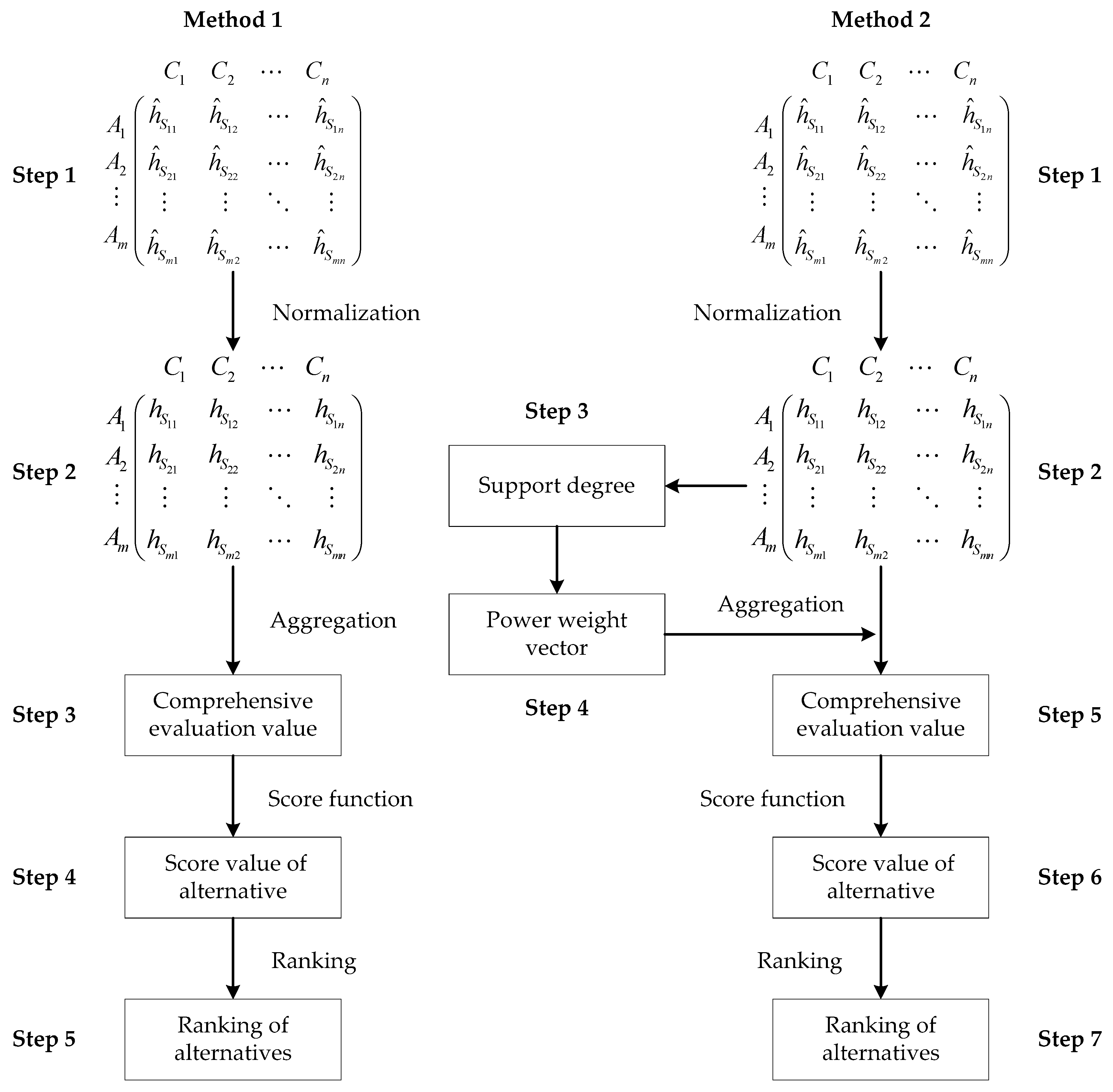
In order to yield the best alternative, the GHFLHWA operator or the GHFLHWG operator, which was developed based on the Hamacher operations, is utilized for the proposed MCDM approach under the hesitant fuzzy linguistic environment. The proposed method includes the following steps.

Method 1.

(The flowchart of Method 1 is shown in Figure 1.)

Step 1.

Determine the linguistic term set that is applied to evaluate each alternative with respect to each criterion; then the hesitant fuzzy linguistic evaluation matrix ${\widehat{H}}_S={({\widehat{h}}_{S_{ij}})}_{m\times n}$ is obtained.

Step 2.

Normalized the evaluation matrix ${\widehat{H}}_S={({\widehat{h}}_{S_{ij}})}_{m\times n}$ according to Equation (33).

Step 3.

Aggregate the criteria values by the GHFLHWA or GHFLHWG operator as follow:

$$h_{S_i}=GHFLHWA(h_{S_{i1}},h_{S_{i2}},\cdots ,h_{S_{in}})\mathrm{or}{h}_{S_i}=GHFLHWG(h_{S_{i1}},h_{S_{i2}},\cdots ,h_{S_{in}})$$

(34)

Step 4.

Compute the score value of each alternative by Equation (2).

Step 5.

Obtained the ranking order of alternatives by the decreasing of the score value.

To reflect the correlation between the input arguments in MCDM problem, we use the GHFLHPWA or GHFLHPWG operator for the proposed MCDM approach. The steps involved are depicted as follows.

Method 2.

(The flowchart of Method 2 is shown in Figure 1.)

Step 1.

Determine the linguistic term set that is applied to evaluate each alternative with respect to each criterion; then the hesitant fuzzy linguistic evaluation matrix ${\widehat{H}}_S={({\widehat{h}}_{S_{ij}})}_{m\times n}$ is obtained.

Step 2.

Normalize the evaluation matrix ${\widehat{H}}_S={({\widehat{h}}_{S_{ij}})}_{m\times n}$ according to Equation (33).

Step 3.

Calculate the support degree of $h_{S_i}$ using the following formula.

$$T(h_{S_{ij}})={\displaystyle {\sum }_{j=1,k\ne j}^{n}Sup(h_{S_{ij}},h_{S_{ik}})}$$

(35)

$$Sup(h_{S_{ij}},h_{S_{ik}})=1-d(h_{S_{ij}},h_{S_{ik}})$$

(36)

Step 4.

Obtained the power weight vector p by the following formula.

$$p_{ij}=w_j(1+T(h_{S_{ij}}))/{\displaystyle {\sum }_{j=1}^n{w}_j(1+T(h_{S_{ij}}))}$$

(37)

Step 5.

Aggregate the criteria values by the GHFLHPWA or GHFLHPWG operators.

$$h_{S_i}=GHFLHPWA(h_{S_{i1}},h_{S_{i2}},\cdots ,h_{S_{in}})\mathrm{or}{h}_{S_i}=GHFLHPWG(h_{S_{i1}},h_{S_{i2}},\cdots ,h_{S_{in}})$$

(38)

Step 6.

Compute the score value of each alternative by Equation (2).

Step 7.

Determined the priority order of alternatives by the decreasing of score value.

6. An Application of the Proposed Operators to MCDM

6.1. Numeric Example

A board of directors of a venture capital company is planning to choose a suitable city to invest in a project of sharing cars in the next three years. The venture capital company determined four alternative cities $A_i(i=1,2,3,4)$ through preliminary market research. In order to evaluate and rank these cities, four criteria (all of them are benefit criteria) are identified by the board of directors including the economic development level ($C_1$), the public transportation development level ($C_2$), the number of public parking lots ($C_3$), and the urban road resources ($C_4$). Assume that the weight vector of these criteria is $w={(0.3,0.1,0.4,0.2)}^{\text{T}}$.

In what follows, we employ Method 1 to determine the most suitable city without considering the correlations of the input arguments.

Step 1.

The board of directors constructs a nine-point linguistic term set to evaluate the ratings of cities, that is, $S=\{s_{-4}=worst,s_{-3}=verybad,s_{-2}=bad,s_{-1}=slightlybad,s_0=medium,s_1=slightlygood,s_2=good,s_3=verygood,s_4=best\}$. Then the decision makers utilize the linguistic term to evaluate the ratings of the cities and the obtained hesitant fuzzy linguistic evaluation matrix ${\widehat{H}}_S={({\widehat{h}}_{S_{ij}})}_{m\times n}$ is presented in

Table 1. The hesitant fuzzy linguistic evaluation matrix.

Cities	${\mathit{C}}_1$	${\mathit{C}}_2$	${\mathit{C}}_3$	${\mathit{C}}_4$
$A_1$	$\{s_0,s_1\}$	$\{s_0\}$	$\{s_1,s_2\}$	$\{s_{-2},s_{-1}\}$
$A_2$	$\{s_1,s_2\}$	$\{s_2,s_3\}$	$\{s_2\}$	$\{s_{-1},s_1\}$
$A_3$	$\{s_1\}$	$\{s_0,s_1\}$	$\{s_1,s_2\}$	$\{s_0,s_1\}$
$A_4$	$\{s_2,s_3\}$	$\{s_0,s_2\}$	$\{s_1,s_3\}$	$\{s_2\}$

.

Step 2.

Since these criteria are all benefit criterions, the evaluate matrix ${\widehat{H}}_S={({\widehat{h}}_{S_{ij}})}_{m\times n}$ is not necessary to be normalized.

Step 3.

Let $\lambda =2$ and $\upsilon =3$, aggregate all of the criteria evaluation values according to the GHFLHWA operator into the total evaluation value $h_{S_i}(i=1,2,3,4)$ of alternative $A_i(i=1,2,3,4)$.

Step 4.

Calculate the score values $s(h_{S_i})$ of $h_{S_i}$ by Definition 6.The obtained results are as follows:

$$s(h_{S_1})=0.5080, s(h_{S_2})=0.6534, s(h_{S_3})=0.5685, s(h_{S_4})=0.7340$$

Step 5.

Based on the decreasing order of score values, we have $h_{S_4}>h_{S_2}>h_{S_3}>h_{S_1}$. Therefore, the best city is $A_4$.

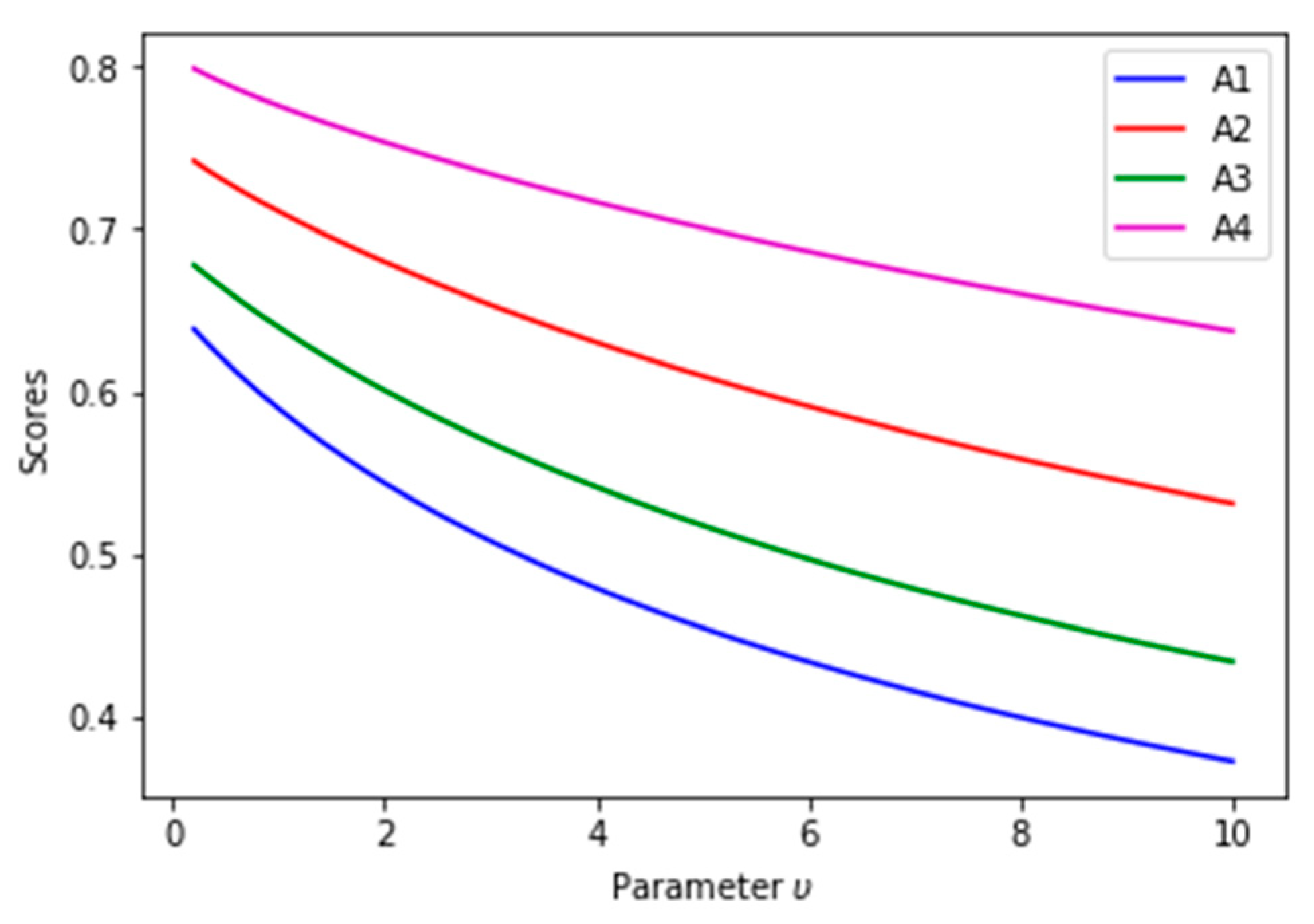
The parameter $\upsilon$ in the GHFLHWA operator indicates the experts’ preference over the alternative with respect to each criterion. In order to explore how the different preference parameter $\upsilon$ in the GHFLHWA operator influences the score values of the alternatives, we utilized different values of $\upsilon \in (0,10]$, which are commonly determined by decision makers. The relative results are shown in Figure 2. It is easy to observe from Figure 2 that the score values of the alternatives become smaller with the increasing values of parameter $\upsilon$. In addition, for the GHFLHWA operator, we can also ascertain from Figure 2 that the final ranking of alternatives for the different parameter $\upsilon$ values does not change. Therefore, the value of parameter $\upsilon$ can be chosen by the decision maker according to their preference.

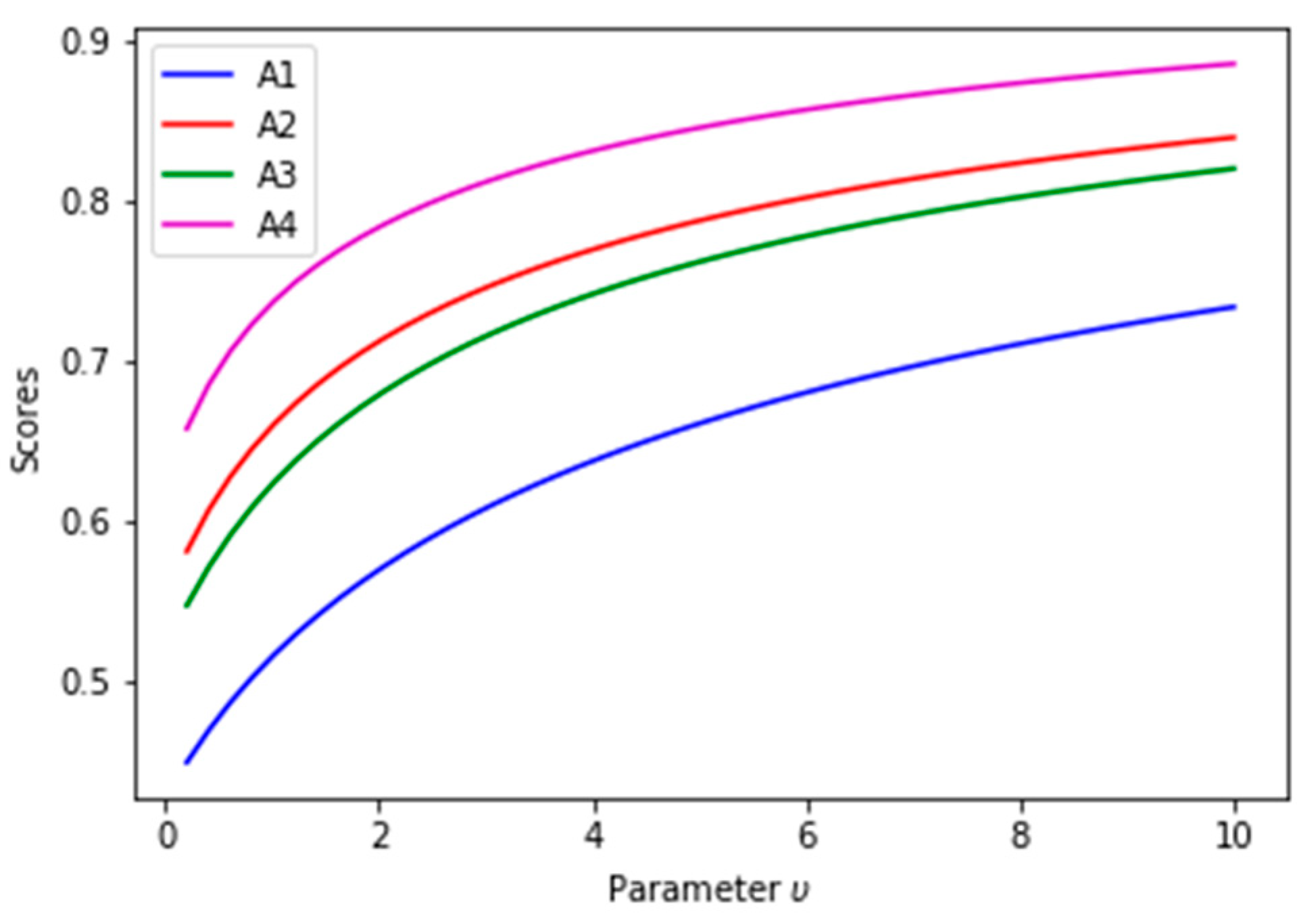
If we use the GHFLHWG operator instead of the GHFLHWA operator to aggregate the criteria values, the variation of score values of the alternatives is shown in Figure 3. From Figure 3, for the GHFLHWG operator, we can see that the score values of the alternatives become greater with the increase of parameter $\upsilon$, which is just the opposite of the GHFLHWA operator. Furthermore, the priority order of alternatives is also not influenced by the different values of parameter $\upsilon$.

When the relationships of the input data are taken into account, we apply Method 2 to resolve the above numerical example.

The first two steps are the same as Method 1.

Step 3.

Compute the support degree $Sup(h_{S_j},h_{S_k})(j=1,2,3,4;j\ne k)$.

$$\begin{array}{cc}Su{p}_{1j}=\left[\begin{array}{cccc}0& 0.9116& 0.8750& 0.7500\\ 0.9116& 0& 0.8024& 0.8024\\ 0.8750& 0.8024& 0& 0.6250\\ 0.7500& 0.8024& 0.6250& 0\end{array}\right],& Su{p}_{2j}=\left[\begin{array}{cccc}0& 0.8750& 0.9116& 0.8024\\ 0.8750& 0& 0.9116& 0.6813\\ 0.9116& 0.9116& 0& 0.7205\\ 0.8024& 0.6813& 0.7205& 0\end{array}\right]\\ Su{p}_{3j}=\left[\begin{array}{cccc}0& 0.9116& 0.9116& 0.9116\\ 0.9116& 0& 0.8750& 1\\ 0.9116& 0.8750& 0& 0.8750\\ 0.9116& 1& 0.8750& 0\end{array},\right]& Su{p}_{4j}=\left[\begin{array}{cccc}0& 0.8024& 0.9116& 0.9116\\ 0.8024& 0& 0.8750& 0.8232\\ 0.9116& 0.8750& 0& 0.8750\\ 0.9116& 0.8232& 0.8750& 0\end{array}\right]\end{array}$$

then

$$T=\left[\begin{array}{cccc}2.5366& 2.5163& 2.3024& 2.1774\\ 2.5890& 2.4679& 2.5437& 2.2042\\ 2.7348& 2.7866& 2.6616& 2.7866\\ 2.6256& 2.5006& 2.6616& 2.6908\end{array}\right]$$

Step 4.

Calculate the power weight matrix.

$$P=\left[\begin{array}{cccc}0.3149& 0.1044& 0.3921& 0.1886\\ 0.3092& 0.0996& 0.4071& 0.1841\\ 0.3011& 0.1018& 0.3936& 0.2035\\ 0.3001& 0.0966& 0.4041& 0.1992\end{array}\right]$$

Step 5.

Let $\lambda =2$ and $\upsilon =3$, aggregate all of the criteria values into the total evaluation value $h_{S_i}(i=1,2,3,4)$ of alternative $A_i(i=1,2,3,4)$ by the GHFLHPWA operator.

Step 6.

Calculate the score values $s(h_{S_i})$ of $h_{S_i}$ by Definition 6; the obtained results are as follows: $s(h_{S_1})=0.5085$, $s(h_{S_2})=0.6563$, $s(h_{S_3})=0.5677$, $s(h_{S_4})=0.7344$.

Step 7.

Based on the decreasing order of score values, we have $h_{S_4}>h_{S_2}>h_{S_3}>h_{S_1}$. Therefore, the best city is $A_4$.

When $\lambda =2$, let $\upsilon =0.1,0.7,2,5,9$, respectively. From one hand, the score values and priority orders of all alternatives determined by the GHFLHPWA operator are shown in

Table 2. The score values and rankings of alternatives obtained by the GHFLHPWA operator.

GHFLHPWA	${\mathit{A}}_1$	${\mathit{A}}_2$	${\mathit{A}}_3$	${\mathit{A}}_4$	Ranking
$GHFLHPW{A}_w^{0.1}$	0.6464	0.7480	0.6832	0.8034	$A_4>A_2>A_3>A_1$
$GHFLHPW{A}_w^{0.7}$	0.6066	0.7231	0.6529	0.7843	$A_4>A_2>A_3>A_1$
$GHFLHPW{A}_w^2$	0.5441	0.6816	0.6005	0.7542	$A_4>A_2>A_3>A_1$
$GHFLHPW{A}_w^5$	0.4550	0.6118	0.5173	0.7016	$A_4>A_2>A_3>A_1$
$GHFLHPW{A}_w^9$	0.3856	0.5467	0.4470	0.6493	$A_4>A_2>A_3>A_1$

. When the value of parameter $\upsilon$ becomes greater, we can obtain a smaller score value of the alternative. We can also see that the ranking order of alternatives is not affected by the different values of parameter $\upsilon$.

On the other hand, if the GHFLHPWG operator is employed to replace the GHFLHPWA operator in the above calculation,

Table 3. The score values and rankings of alternatives obtained by the GHFLHPWG operator.

GHFLHPWG	${\mathit{A}}_1$	${\mathit{A}}_2$	${\mathit{A}}_3$	${\mathit{A}}_4$	Ranking
$GHFLHPW{G}_w^{0.1}$	0.4409	0.5693	0.5328	0.6400	$A_4>A_2>A_3>A_1$
$GHFLHPW{G}_w^{0.7}$	0.4969	0.6400	0.5985	0.7143	$A_4>A_2>A_3>A_1$
$GHFLHPW{G}_w^2$	0.5727	0.7162	0.6779	0.7836	$A_4>A_2>A_3>A_1$
$GHFLHPW{G}_w^5$	0.6638	0.7909	0.7608	0.8454	$A_4>A_2>A_3>A_1$
$GHFLHPW{G}_w^9$	0.7253	0.8347	0.8107	0.8796	$A_4>A_2>A_3>A_1$

gives the score values and the final ranking of the alternatives. In Table 3, we can observe that the score values of alternatives become greater when the value of parameter $\upsilon$ increases. In addition, the priority order of alternatives does not change when the value of parameter $\upsilon$ changes. Hence, the ranking order of alternatives is robust for the parameters $\upsilon =0.1,0.7,2,5,9$ in this example.

Based on the above analysis, we can conclude that the priority order of alternatives obtained by the GHFLHWA and GHFLHWG operators are the same as that obtained by the GHFLHPWA and GHFLHPWG operators, that is, the ranking order of alternatives is $A_4>A_2>A_3>A_1$. Further, the results also indicate that the correlations between the input arguments are not enough to affect the ranking order of alternatives in this example.

6.2. Comparison with Existing Methods of Hesitant Fuzzy Linguistic MCDM

In this section, we use the proposed methods comparison with the previously developed HFL MCDM approaches. The previous methods include the proposed approach with Zhang and Wu [24], where the HFL weighted averaging and HFL weighted geometric operators were employed to aggregate the HFL evaluation information, and the HFL TOPSIS method [22].

The linguistic term set in these two methods is subscript-asymmetric, however, the linguistic term set used in this paper is subscript-symmetric. Therefore, we need to transform the evaluation matrix into another form for the use of these two approaches. The transformed HFL evaluation matrix is shown in

Table 4. The transformed hesitant fuzzy linguistic evaluation matrix.

Cities	${\mathit{C}}_1$	${\mathit{C}}_2$	${\mathit{C}}_3$	${\mathit{C}}_4$
$A_1$	$\{s_4,s_5\}$	$\{s_4\}$	$\{s_5,s_6\}$	$\{s_2,s_3\}$
$A_2$	$\{s_5,s_6\}$	$\{s_6,s_7\}$	$\{s_6\}$	$\{s_3,s_5\}$
$A_3$	$\{s_5\}$	$\{s_4,s_5\}$	$\{s_5,s_6\}$	$\{s_4,s_5\}$
$A_4$	$\{s_6,s_7\}$	$\{s_4,s_6\}$	$\{s_5,s_7\}$	$\{s_6\}$

.

In the following, we utilize the HFLWA operator [24] instead of the GHFLHWA operator in Method 1 based on the operational laws in Definition 4 to solve the numerical example. That is

$$h_{S_i}=HFLWA(h_{S_{i1}},h_{S_{i2}},h_{S_{i3}},h_{S_{i4}})=\underset{j=1}{\stackrel{4}{\oplus }}(w_j{h}_{S_{ij}})=\underset{{\sigma }_{ij}\in g(h_{S_{ij}})}{\cup }\{g^{-1}\left(1-{\displaystyle {\prod }_{j=1}^4{(1-{\sigma }_{ij})}^{w_j}}\right)\}$$

then, we can obtain the score values of the alternatives as follows:

$$s(h_{S_1})=0.5790, s(h_{S_2})=0.7060, s(h_{S_3})=0.6376, s(h_{S_4})=0.7731$$

In this situation, the priority order of alternatives is $A_4>A_2>A_3>A_1$, and the best city is $A_4$.

If we use the HFLWG operator [24] instead of the GHFLHWA operator in Method 1, we get

$$h_{S_i}=HFLWG(h_{S_{i1}},h_{S_{i2}},h_{S_{i3}},h_{S_{i4}})=\underset{j=1}{\stackrel{4}{\otimes }}{(h_{S_{ij}})}^{w_j}=\underset{{\sigma }_{ij}\in g(h_{S_{ij}})}{\cup }\{g^{-1}\left({\displaystyle {\prod }_{j=1}^n{({\sigma }_{ij})}^{w_j}}\right)\}$$

Then, we can obtain the score values of the alternatives as follows:

$$s(h_{S_1})=0.5326, s(h_{S_2})=0.6749, s(h_{S_3})=0.6275, s(h_{S_4})=0.7094$$

In this situation, the priority order of alternatives is $A_4>A_2>A_3>A_1$, and the best city is $A_4$.

Based on the above analyses, we can see that the best city and the ranking order of alternatives obtained by the HFLWA and HFLWG operators are the same for Methods 1 and 2, which illustrate the validity of Methods 1 and 2. In addition, we should note that the GHFLHWA and GHFLHWG operators reduce to the HFLWA and HFLWG operator, respectively, when $\lambda =1$ and $\upsilon =1$. It indicates that the method based on the GHFLHWA or GHFLHWG operators is more general and flexible than the HFLWA or HFLWG operators.

In the following, we apply the HFL TOPSIS method [22] to solve the numerical example. First, we review the HFL TOPSIS approach as follows:

Step 1.

For an MCDM problem with HFL information, let $X=\{x_1,x_2,\cdots ,x_m\}$ be a collection of m alternatives and $C=\{c_1,c_2,\cdots ,c_n\}$ be a collection of n criteria with weight vector $w={(w_1,w_2,\cdots ,w_n)}^{\mathrm{T}}$ satisfying $w_j\in [0,1]$ and ${\displaystyle {\sum }_{j=1}^n{w}_j}=1$. Suppose $R={(h_{S_{ij}})}_{m\times n}$ is an HFL evaluation matrix provided by the decision makers, where $h_{S_{ij}}$ is an HFLE.

Step 2.

Based on the evaluation matrix R, an HFL positive ideal solution (HFLPIS) and an HFL negative ideal solution (HFLNIS) can be determined by

$$H_S^{+}=(h_{S_1}^{+},h_{S_2}^{+},\cdots ,h_{S_n}^{+})$$

(39)

where $h_{S_j}^{+}=h_{S_{1j}}\vee h_{S_{2j}}\vee \cdots \vee h_{S_{mj}}$ if $c_j$ is a benefit criterion and $h_{S_j}^{+}=h_{S_{1j}}\wedge h_{S_{2j}}\wedge \cdots \wedge h_{S_{mj}}$ if $c_j$ is a cost criterion.

$$H_S^{-}=(h_{S_1}^{-},h_{S_2}^{-},\cdots ,h_{S_n}^{-})$$

(40)

where $h_{S_j}^{-}=h_{S_{1j}}\wedge h_{S_{2j}}\wedge \cdots \wedge h_{S_{mj}}$ if $c_j$ is a benefit criterion and $h_{S_j}^{-}=h_{S_{1j}}\vee h_{S_{2j}}\vee \cdots \vee h_{S_{mj}}$ if $c_j$ is a cost criterion. Where $\vee$ and $\wedge$ are defined by Definition 3 [22].

Step 3.

The distance from each alternative to HFLPIS and HFLNIS are calculated as follows:

$$d_i^{+}={\displaystyle {\sum }_{j=1}^n{w}_{j}d(h_{S_{ij}},h_{S_j}^{+})}$$

(41)

$$d_i^{-}={\displaystyle {\sum }_{j=1}^n{w}_{j}d(h_{S_{ij}},h_{S_j}^{-})}$$

(42)

where $d(h_{S_{ij}},h_{S_j}^{+})$ and $d(h_{S_{ij}},h_{S_j}^{-})$ are determined by Definition 7.

Step 4.

The closeness coefficients $d_i$ of alternatives $x_i$ can be calculated by

$$c{c}_i=\frac{d_i^{-}}{d_i^{+}+d_i^{-}}$$

(43)

Step 5.

Determine the priority orders of all alternatives in the light of the decrease of the closeness coefficient $d_i$.

In what follows, we utilize the HFL TOPSIS approach to resolve the numerical example. The detailed steps are described as follows:

Step 1.

The hesitant fuzzy linguistic evaluation matrix R is shown in Table 4.

Step 2.

Based on the hesitant fuzzy linguistic evaluation matrix R, the HFLPIS and the HFLNIS are determined as

$$H_S^{+}=(\{s_6,s_7\},\{s_6,s_7\},\{s_6,s_7\},\{s_6\})$$

$$H_S^{-}=(\{s_4,s_5\},\{s_4\},\{s_5,s_6\},\{s_2,s_3\})$$

Step 3.

The distance from each alternative to HFLPIS and HFLNIS are obtained as

$$d_1^{+}=0.2453, d_2^{+}=0.1288, d_3^{+}=0.1738, d_4^{+}=0.0551$$

$$d_1^{-}=0.0000, d_2^{-}=0.1443, d_3^{-}=0.0854, d_4^{-}=0.2164$$

Step 4.

Employ Equation (43) to compute the closeness coefficient of alternative $x_i$.

$$c{c}_1=0.0000, c{c}_2=0.5284, c{c}_3=0.3293, c{c}_4=0.7970$$

Step 5.

The final priority order of all alternatives obtained as follows: $A_4>A_2>A_3>A_1$.

Based on the above calculation, we can see that the best city is $A_4$.

From the obtained results above, we can ascertain that the results determined by the HFL TOPSIS are the same as that of the proposed methods, which also validates the effectiveness of the presented methods in this paper. Furthermore, the GHFLHPWA or GHFLHPWG operators in Method 2 consider the relationships between the input arguments through the weight vector determined by the support degree.

Compared with the HFLWA or HFLWG operators and the HFL TOPSIS method, the presented Methods in this paper have the following two advantages. First, decision makers can determine the parameter value $\upsilon$ in the operators of Methods1 and 2 according to their subjective preferences, which increases the flexibility of the proposed methods to handle practical decision-making problems. Second, Method 2 reduces the influences of unreasonable input arguments by using the support measure assigning a lower weight to them and reflects the correlations between the input arguments by applying the weight vector allowing the input arguments to support and reinforce each other, both of which rendering the decision result more reasonable.

7. Conclusions

This paper investigates the information aggregation problem of MCDM problems in which the value of the criterion is expressed with HFLEs. Inspired by the idea of Hamacher t-norm and t-conorm, we defined some new basic operational laws on HFLEs based on the Hamacher t-norm and t-conorm. Then, based on these operational laws, we present several hesitant fuzzy linguistic Hamacher aggregation operators which are more general and flexible aggregation operators, including the HFLHWA, HFLHWG, GHFLHWA, GHFLHWG, HFLHPWA, HFLHPWG, GHFLHPWA, and GHFLHPWG operators. We also discuss some special cases of these operators and explore some of their desirable properties. Further, we propose two methods based on the GHFLHWA, GHFLHWG, GHFLHPWA, and GHFLHPWG operators to deal with the MCDM problem with HFLE information. Ultimately, a numerical example is provided to demonstrate the process of the developed methodology, and the influence of distinct parameters $\upsilon$ on the score function of the alternative is discussed. In the future, we will extend the presented operators to other uncertain environments and apply these operators to other fields, such as supply chain management, risk management, and fuzzy cluster analysis.

References

- Zadeh, L.A. Fuzzy sets. Inf. Control 1965, 8, 338–353. [Google Scholar] [CrossRef]
- Zadeh, L.A. The concept of a linguistic variable and its application to approximate reasoning—I. Inf. Sci. 1974, 8, 199–249. [Google Scholar] [CrossRef]
- Atanassov, K.T.; Rangasamy, P. Intuitionistic fuzzy sets. Fuzzy Sets Syst. 1986, 20, 87–96. [Google Scholar] [CrossRef]
- Atannasov, K. Intuitionistic Fuzzy Sets: Theory and Applications; Physica-Verlag: Heidelberg, Germany, 1999. [Google Scholar]
- Yager, R.R. Pythagorean fuzzy subsets. In Proceedings of the IFSA World Congress and NAFIPS Annual Meeting, Edmonton, AB, Canada, 24–28 June 2013; pp. 57–61. [Google Scholar]
- Yager, R.R. Pythagorean membership grades in multicriteria decision making. IEEE Trans. Fuzzy Syst. 2014, 22, 958–965. [Google Scholar] [CrossRef]
- Dubois, D.; Prade, H. Fuzzy Sets and Systems: Theory and Applications; Academic Press: Cambridge, MA, USA, 1980; pp. 370–374. [Google Scholar]
- Mizumoto, M.; Tanaka, K. Fuzzy sets and type 2 under algebraic product and algebraic sum. Fuzzy Sets Syst. 1981, 5, 277–290. [Google Scholar] [CrossRef]
- Yager, R.R. On the theory of bags. Int. J. Gen. Syst. 1986, 13, 23–37. [Google Scholar] [CrossRef]
- Torra, V.; Narukawa, Y. On hesitant fuzzy sets and decision. In Proceedings of the 18th IEEE International Conference on Fuzzy Systems, Jeju lsland, Korea, 20–24 August 2009; pp. 1378–1382. [Google Scholar]
- Torra, V. Hesitant fuzzy sets. Int. J. Intell. Syst. 2010, 25, 529–539. [Google Scholar] [CrossRef]
- Zadeh, L.A. The concept of a linguistic variable and its application to approximate reasoning—II. Inf. Sci. 1975, 8, 301–357. [Google Scholar] [CrossRef]
- Zadeh, L.A. The concept of a linguistic variable and its application to approximate reasoning—III. Inf. Sci. 1975, 9, 43–80. [Google Scholar] [CrossRef]
- Ciasullo, M.V.; Fenza, G.; Loia, V.; Orciuoli, F.; Troisi, O.; Herrera-Viedma, E. Business process outsourcing enhanced by fuzzy linguistic consensus model. Appl. Soft Comput. 2018, 64, 436–444. [Google Scholar] [CrossRef]
- Cui, J. Model for evaluating the security of wireless network with fuzzy linguistic information. J. Intell. Fuzzy Syst. 2017, 32, 2697–2704. [Google Scholar] [CrossRef]
- Peiris, H.O.W.; Chakraverty, S.; Perera, S.S.N.; Ranwala, S.M.W. Novel fuzzy linguistic based mathematical model to assess risk of invasive alien plant species. Appl. Soft Comput. 2017, 59, 326–339. [Google Scholar] [CrossRef]
- Wang, G.; Tian, X.; Hu, Y.; Evans, R.D.; Tian, M.; Wang, R. Manufacturing process innovation-oriented knowledge evaluation using mcdm and fuzzy linguistic computing in an open innovation environment. Sustainability 2017, 9, 1630. [Google Scholar] [CrossRef]
- Pei, Z.; Liu, J.; Hao, F.; Zhou, B. Flm-topsis: The fuzzy linguistic multiset topsis method and its application in linguistic decision making. Inf. Fusion 2018, 45, 266–281. [Google Scholar] [CrossRef]
- Rodriguez, R.M.; Martinez, L.; Herrera, F. Hesitant fuzzy linguistic term sets for decision making. IEEE Trans. Fuzzy Syst. 2012, 20, 109–119. [Google Scholar] [CrossRef]
- Liao, H.; Xu, Z.; Zeng, X.J. Qualitative decision making with correlation coefficients of hesitant fuzzy linguistic term sets. Knowl. Based Syst. 2015, 76, 127–138. [Google Scholar] [CrossRef]
- Zhang, B.; Liang, H.; Zhang, G. Reaching a consensus with minimum adjustment in magdm with hesitant fuzzy linguistic term sets. Inf. Fusion 2017, 42, 12–23. [Google Scholar] [CrossRef]
- Wei, C.; Zhao, N.; Tang, X. Operators and comparisons of hesitant fuzzy linguistic term sets. IEEE Trans. Fuzzy Syst. 2014, 22, 575–585. [Google Scholar] [CrossRef]
- Lee, L.W.; Chen, S.M. Fuzzy decision making based on likelihood-based comparison relations of hesitant fuzzy linguistic term sets and hesitant fuzzy linguistic operators. Inf. Sci. 2015, 294, 513–529. [Google Scholar] [CrossRef]
- Zhang, Z.; Wu, C. Hesitant fuzzy linguistic aggregation operators and their applications to multiple attribute group decision making. J. Intell. Fuzzy Syst. 2014, 26, 2185–2202. [Google Scholar]
- Wang, H. Extended hesitant fuzzy linguistic term sets and their aggregation in group decision making. Int. J. Comput. Intell. Syst. 2015, 8, 14–33. [Google Scholar] [CrossRef]
- Shi, M.; Xiao, Q. Hesitant fuzzy linguistic aggregation operators based on global vision. J. Intell. Fuzzy Syst. 2017, 33, 193–206. [Google Scholar] [CrossRef]
- Xu, Y.; Xu, A.; Merigó, J.M.; Wang, H. Hesitant fuzzy linguistic ordered weighted distance operators for group decision making. J. Appl. Math. Comput. 2015, 49, 285–308. [Google Scholar] [CrossRef]
- Liu, X.; Zhu, J.; Zhang, S.; Liu, G. Multiple attribute group decision-making methods under hesitant fuzzy linguistic environment. J. Intell. Syst. 2017, 26, 387–406. [Google Scholar] [CrossRef]
- Zhang, J.L.; Qi, X.W. In Research on multiple attribute decision making under hesitant fuzzy linguistic environment with application to production strategy decision making. In Advanced Materials Research; Trans Tech Publications: Zürich, Switzerland, 2013; Volume 753–755, pp. 2829–2836. [Google Scholar]
- Gou, X.; Xu, Z.; Liao, H. Multiple criteria decision making based on bonferroni means with hesitant fuzzy linguistic information. Soft Comput. 2017, 21, 6515–6529. [Google Scholar] [CrossRef]
- Wang, W.; Liu, X. Intuitionistic fuzzy information aggregation using Einstein operations. IEEE Trans. Fuzzy Syst. 2012, 20, 923–938. [Google Scholar] [CrossRef]
- Wang, W.; Liu, X. Intuitionistic fuzzy geometric aggregation operators based on Einstein operations. Int. J. Intell. Syst. 2011, 26, 1049–1075. [Google Scholar] [CrossRef]
- Zhang, Z. Multi-criteria group decision-making methods based on new intuitionistic fuzzy Einstein hybrid weighted aggregation operators. Neural Comput. Appl. 2017, 28, 3781–3800. [Google Scholar] [CrossRef]
- Yu, D. Some hesitant fuzzy information aggregation operators based on Einstein operational laws. Int. J. Intell. Syst. 2014, 29, 320–340. [Google Scholar] [CrossRef]
- Jin, F.; Ni, Z.; Chen, H. Interval-Valued Hesitant Fuzzy Einstein Prioritized Aggregation Operators and Their Applications to Multi-Attribute Group Decision Making; Springer-Verlag: Berlin, Germany, 2016; pp. 1863–1878. [Google Scholar]
- Hamacher, H. Uber logische verknunpfungenn unssharfer aussagen undderen zugenhorige bewertungsfunktione. Prog. Cybern. Syst. Res. 1978, 3, 267–288. [Google Scholar]
- Tan, C.; Yi, W.; Chen, X. Hesitant fuzzy hamacher aggregation operators for multicriteria decision making. Appl. Soft Comput. 2015, 26, 325–349. [Google Scholar] [CrossRef]
- Ju, Y.; Zhang, W.; Yang, S. Some dual hesitant fuzzy hamacher aggregation operators and their applications to multiple attribute decision making. J. Intell. Fuzzy Syst. 2014, 27, 2481–2495. [Google Scholar]
- Liu, J.; Zhou, N.; Zhuang, L.H.; Li, N.; Jin, F.F. Interval-valued hesitant fuzzy multiattribute group decision making based on improved hamacher aggregation operators and continuous entropy. Math. Probl. Eng. 2017, 2017, 2931482. [Google Scholar] [CrossRef]
- Huang, J.Y. Intuitionistic fuzzy hamacher aggregation operators and their application to multiple attribute decision making. J. Intell. Fuzzy Syst. 2014, 27, 505–513. [Google Scholar]
- Liu, P. Some hamacher aggregation operators based on the interval-valued intuitionistic fuzzy numbers and their application to group decision making. IEEE Trans. Fuzzy Syst. 2014, 22, 83–97. [Google Scholar] [CrossRef]
- Wei, G.; Lu, M.; Tang, X.; Wei, Y. Pythagorean hesitant fuzzy hamacher aggregation operators and their application to multiple attribute decision making. Int. J. Intell. Syst. 2018, 33, 1197–1233. [Google Scholar] [CrossRef]
- Wu, Q.; Wu, P.; Zhou, L.; Chen, H.; Guan, X. Some new Hamacher aggregation operators under single-valued neutrosophic 2-tuple linguistic environment and their applications to multi-attribute group decision making. Comput. Ind. Eng. 2018, 116, 144–162. [Google Scholar] [CrossRef]
- Yager, R.R. The power average operator. IEEE Trans. Syst. Man Cybern. Part A Syst. Hum. 2001, 31, 724–731. [Google Scholar] [CrossRef]
- Xu, Z.; Yager, R.R. Power-geometric operators and their use in group decision making. IEEE Trans. Fuzzy Syst. 2010, 18, 94–105. [Google Scholar]
- Xu, Z. Approaches to multiple attribute group decision making based on intuitionistic fuzzy power aggregation operators. Knowl. Based Syst. 2011, 24, 749–760. [Google Scholar] [CrossRef]
- Wei, G.; Lu, M. Pythagorean fuzzy power aggregation operators in multiple attribute decision making. Int. J. Intell. Syst. 2018, 33, 169–186. [Google Scholar] [CrossRef]
- Zhang, Z. Hesitant fuzzy power aggregation operators and their application to multiple attribute group decision making. Inf. Sci. 2013, 234, 150–181. [Google Scholar] [CrossRef]
- Jiang, W.; Wei, B.; Liu, X.; Li, X.; Zheng, H. Intuitionistic fuzzy power aggregation operator based on entropy and its application in decision making. Int. J. Intell. Syst. 2018, 33, 49–67. [Google Scholar] [CrossRef]
- Zhu, C.; Zhu, L.; Zhang, X. Linguistic hesitant fuzzy power aggregation operators and their applications in multiple attribute decision-making. Inf. Sci. 2016, 367, 809–826. [Google Scholar] [CrossRef]
- Liu, P.; Qin, X. Power average operators of linguistic intuitionistic fuzzy numbers and their application to multiple-attribute decision making. J. Intell. Fuzzy Syst. 2017, 32, 1029–1043. [Google Scholar] [CrossRef]
- Wang, L.; Shen, Q.; Zhu, L. Dual hesitant fuzzy power aggregation operators based on archimedean t-conorm and t-norm and their application to multiple attribute group decision making. Appl. Soft Comput. 2016, 38, 23–50. [Google Scholar] [CrossRef]
- Liu, C.; Luo, Y. Power aggregation operators of simplified neutrosophic sets and their use in multi-attribute group decision making. IEEE/CAA J. Autom. Sin. 2017. [Google Scholar] [CrossRef]
- Deschrijver, G.; Cornelis, C.; Kerre, E.E. On the representation of intuitionistic fuzzy t-norms and t-conorms. IEEE Trans. Fuzzy Syst. 2004, 12, 45–61. [Google Scholar] [CrossRef]
- Klement, E.P.; Mesiar, R.; Pap, E. Triangular norms. Position paper I: Basic analytical and algebraic properties. Fuzzy Sets Syst. 2004, 143, 5–26. [Google Scholar] [CrossRef]
- Jenei, S. A note on the ordinal sum theorem and its consequence for the construction of triangular norms. Fuzzy Sets Syst. 2002, 126, 199–205. [Google Scholar] [CrossRef]
- Gou, X.; Xu, Z. Novel basic operational laws for linguistic terms, hesitant fuzzy linguistic term sets and probabilistic linguistic term sets. Inf. Sci. 2016, 372, 407–427. [Google Scholar] [CrossRef]
- Gou, X.; Xu, Z.; Liao, H. Group decision making with compatibility measures of hesitant fuzzy linguistic preference relations. Soft Comput. 2017. [Google Scholar] [CrossRef]
- Torra, V.; Narukawa, Y. Modeling decisions—Information fusion and aggregation operators. Cogn. Technol. 2007, 61, 1090–1093. [Google Scholar]
Figure 1.
The flowcharts of the Method 1 and Method 2.
Figure 2.
The variation of score values of alternatives with regard to in the GHFLHWA operator.
Figure 3.
The variation of score values of alternatives with regard to in the GHFLHWG operator.