A Study on Neutrosophic Cubic Graphs with Real Life Applications in Industries
by
 , , and
Muhammad Gulistan
1 ,
,
Naveed Yaqoob
2,
Zunaira Rashid
1,*,
Florentin Smarandache
3 and
and
Hafiz Abdul Wahab
1 1
Department of Mathematics, Hazara University, Mansehra 21120, Pakistan
2
Department of Mathematics, College of Science, Majmaah University, Al-Zulfi 11952, Saudi Arabia
3
Department of Mathematics, University of New Mexico, Albuquerque, NM 87301, USA
*
Author to whom correspondence should be addressed.
Symmetry 2018, 10(6), 203; https://doi.org/10.3390/sym10060203
Submission received: 27 April 2018
/
Revised: 29 May 2018
/
Accepted: 30 May 2018
/
Published: 5 June 2018
(This article belongs to the Special Issue Algebraic Structures of Neutrosophic Triplets, Neutrosophic Duplets, or Neutrosophic Multisets)
Abstract
:Neutrosophic cubic sets are the more generalized tool by which one can handle imprecise information in a more effective way as compared to fuzzy sets and all other versions of fuzzy sets. Neutrosophic cubic sets have the more flexibility, precision and compatibility to the system as compared to previous existing fuzzy models. On the other hand the graphs represent a problem physically in the form of diagrams, matrices etc. which is very easy to understand and handle. So the authors applied the Neutrosophic cubic sets to graph theory in order to develop a more general approach where they can model imprecise information through graphs. We develop this model by introducing the idea of neutrosophic cubic graphs and introduce many fundamental binary operations like cartesian product, composition, union, join of neutrosophic cubic graphs, degree and order of neutrosophic cubic graphs and some results related with neutrosophic cubic graphs. One of very important futures of two neutrosophic cubic sets is the R-union that R-union of two neutrosophic cubic sets is again a neutrosophic cubic set, but here in our case we observe that R-union of two neutrosophic cubic graphs need not be a neutrosophic cubic graph. Since the purpose of this new model is to capture the uncertainty, so we provide applications in industries to test the applicability of our defined model based on present time and future prediction which is the main advantage of neutrosophic cubic sets.
Keywords:
neutrosophic cubic set; neutrosophic cubic graphs; applications of neutrosophic cubic graphsMSC:
68R10; 05C72; 03E721. Introduction
In 1965, Zadeh [1] published his seminal paper “Fuzzy Sets” which described fuzzy set theory and consequently fuzzy logic. The purpose of Zadeh’s paper was to develop a theory which could deal with ambiguity and imprecision of certain classes or sets in human thinking, particularly in the domains of pattern recognition, communication of information and abstraction. This theory proposed making the grade of membership of an element in a subset of a universal set a value in the closed interval of real numbers. Zadeh’s ideas have found applications in computer sciences, artificial intelligence, decision analysis, information sciences, system sciences, control engineering, expert systems, pattern recognition, management sciences, operations research and robotics. Theoretical mathematics has also been touched by fuzzy set theory. The ideas of fuzzy set theory have been introduced into topology, abstract algebra, geometry, graph theory and analysis. Further, he made the extension of fuzzy set to interval-valued fuzzy sets in 1975, where one is not bound to give a specific membership to a certain element. In 1975, Rosenfeld [2] discussed the concept of fuzzy graphs whose basic idea was introduced by Kauffmann [3] in 1973. The fuzzy relations between fuzzy sets were also considered by Rosenfeld and he developed the structure of fuzzy graphs obtaining analogs of several graph theoretical concepts [4]. Bhattacharya provided further studies on fuzzy graphs [5]. Akram and Dudek gave the idea of interval valued fuzzy graphs in 2011 where they used interval membership for an element in the vertex set [6]. Akram further extended the idea of interval valued fuzzy graphs to Interval-valued fuzzy line graphs in 2012. More detail of fuzzy graphs, we refer the reader to [7,8,9,10,11,12]. In 1986, Atanassov [13] use the notion of membership and non-membership of an element in a set X and gave the idea of intuitionistic fuzzy sets. He extended this idea to intuitionistic fuzzy graphs and for more detail in this direction, we refer the reader to [14,15,16,17,18,19,20]. Akram and Davvaz [21] introduced the notion of strong intuitionistic fuzzy graphs and investigated some of their properties. They discussed some propositions of self complementary and self weak complementary strong intuitionistic fuzzy graphs. In 1994, Zhang [22] started the theory of bipolar fuzzy sets as a generality of fuzzy sets. Bipolar fuzzy sets are postponement of fuzzy sets whose membership degree range is . Akram [23,24] introduced the concepts of bipolar fuzzy graphs, where he introduced the notion of bipolar fuzzy graphs, described various methods of their construction, discussed the concept of isomorphisms of these graphs and investigated some of their important properties. He then introduced the notion of strong bipolar fuzzy graphs and studied some of their properties. He also discussed some propositions of self complementary and self weak complementary strong bipolar fuzzy graphs and applications, for example see [25]. Smarandache [26,27,28] extended the concept of Atanassov and gave the idea of neutrosophic sets. He proposed the term “neutrosophic” because “neutrosophic” etymologically comes from “neutrosophy” This comes from the French neutre < Latin neuter, neutral, and Greek sophia, skill/wisdom, which means knowledge of neutral thought, and this third/neutral represents the main distinction between “fuzzy” and “intuitionistic fuzzy” logic/set, i.e., the included middle component (Lupasco-Nicolescu’s logic in philosophy), i.e., the neutral/indeterminate/unknown part (besides the “truth”/“membership” and “falsehood”/“non-membership” components that both appear in fuzzy logic/set). See the Proceedings of the First International Conference on Neutrosophic Logic, The University of New Mexico, Gallup Campus, 1–3 December 2001, at http://www.gallup.unm.edu/~smarandache/FirstNeutConf.htm.
After that, many researchers used the idea of neutrosophic sets in different directions. The idea of neutrosophic graphs is provided by Kandasamy et al. in the book title as Neutrosophic graphs, where they introduce idea of neutrosophic graphs [29]. This study reveals that these neutrosophic graphs give a new dimension to graph theory. An important feature of this book is that it contains over 200 neutrosophic graphs to provide better understandings of these concepts. Akram and others discussed different aspects of neutrosophic graphs [30,31,32,33]. Further Jun et al. [34] gave the idea of cubic set and it was characterized by interval valued fuzzy set and fuzzy set, which is more general tool to capture uncertainty and vagueness, while fuzzy set deals with single value membership and interval valued fuzzy set ranges the membership in the form of interval. The hybrid platform provided by the cubic set is the main advantage, in that it contains more information then a fuzzy set and interval valued fuzzy set. By using this concept, we can solve different problems arising in several areas and can pick finest choice by means of cubic sets in various decision making problems. This hybrid nature of the cubic set attracted these researchers to work in this field. For more detail about cubic sets and their applications in different research areas, we refer the reader to [35,36,37]. Recently, Rashid et al. [38] introduced the notion of cubic graphs where they introduced many new types of graphs and provided their application. More recently Jun et al. [39,40] combined neutrosophic set with cubic sets and gave the idea of Neutrosophic cubic set and defined different operations.
Therefore, the need was felt to develop a model for neutrosophic cubic graphs which is a more generalized tool to handle uncertainty. In this paper, we introduce the idea of neutrosophic cubic graphs and introduce the fundamental binary operations, such as the cartesian product, composition, union, join of neutrosophic cubic graphs, degree, order of neutrosophic cubic graphs and some results related to neutrosophic cubic graphs. We observe that R-union of two neutrosophic cubic graphs need not to be a neutrosophic cubic graph. At the end, we provide applications of neutrosophic cubic graphs in industries to test the applicability of our presented model.
2. Preliminaries
We recall some basic definitions related to graphs, fuzzy graphs and neutrosophic cubic sets.
Definition 1.
A graph is an ordered pair , where V is the set of vertices of and E is the set of edges of .
Definition 2.
We call the fuzzy vertex function of V, the fuzzy edge function of respectively. Please note that is a symmetric fuzzy relation on . We use the notation for an element of E. Thus, is a fuzzy graph of if for all .
Definition 3.
Definition 4.
Let and be two fuzzy functions of and and let and be fuzzy functions of and , respectively. The Cartesian product of two fuzzy graphs and [2,3,4] of the graphs and is denoted by and is defined as follows:
- (i)
- for all
- (ii)
- for all , for all .
- (iii)
- for all , for all
Definition 5.
Let and be fuzzy functions of and and let and be fuzzy functions of and , respectively. The composition of two fuzzy graphs and of the graphs and [2,3,4] is denoted by and is defined as follows:
- (i)
- for all .
- (ii)
- for all for all
- (iii)
- for all for all
- (iv)
- for all for all
Definition 6.
Let and be fuzzy functions of and and let and be fuzzy functions of and , respectively. Then union of two fuzzy graphs and of the graphs and [2,3,4] is denoted by and is defined as follows:
- (i)
- if
- (ii)
- if
- (iii)
- if
- (iv)
- if
- (v)
- if
- (vi)
- ( if .
Definition 7.
Let and be fuzzy functions of and and let and be fuzzy functions of and , respectively. Then join of two fuzzy graphs and of the graphs and [2,3,4] is denoted by and is defined as follows:
- (i)
- if
- (ii)
- if
- (iii)
- if .
Definition 8.
Let X be a non-empty set. A neutrosophic cubic set (NCS) in X [39] is a pair where is an interval neutrosophic set in X and is a neutrosophic set in X.
3. Neutrosophic Cubic Graphs
The motivation behind this section is to combine the concept of neutrosophic cubic sets with graphs theory. We introduce the concept of neutrosophic cubic graphs, order and degree of neutrosophic cubic graph and different fundamental operations on neutrosophic cubic graphs with examples.
Definition 9.
Let be a graph. By neutrosophic cubic graph of , we mean a pair where is the neutrosophic cubic set representation of vertex set V and is the neutrosophic cubic set representation of edges set E such that;
- (i)
- (ii)
- (iii)
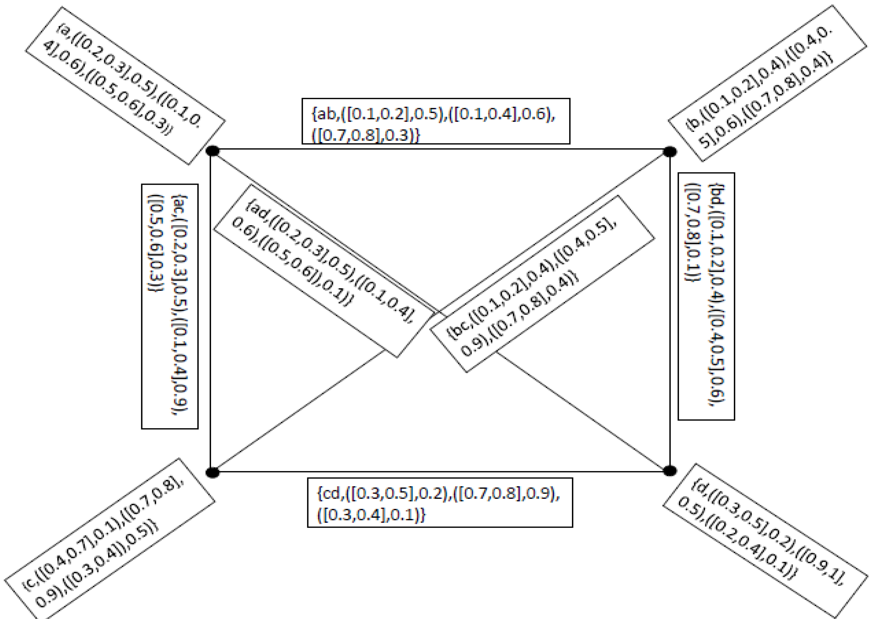
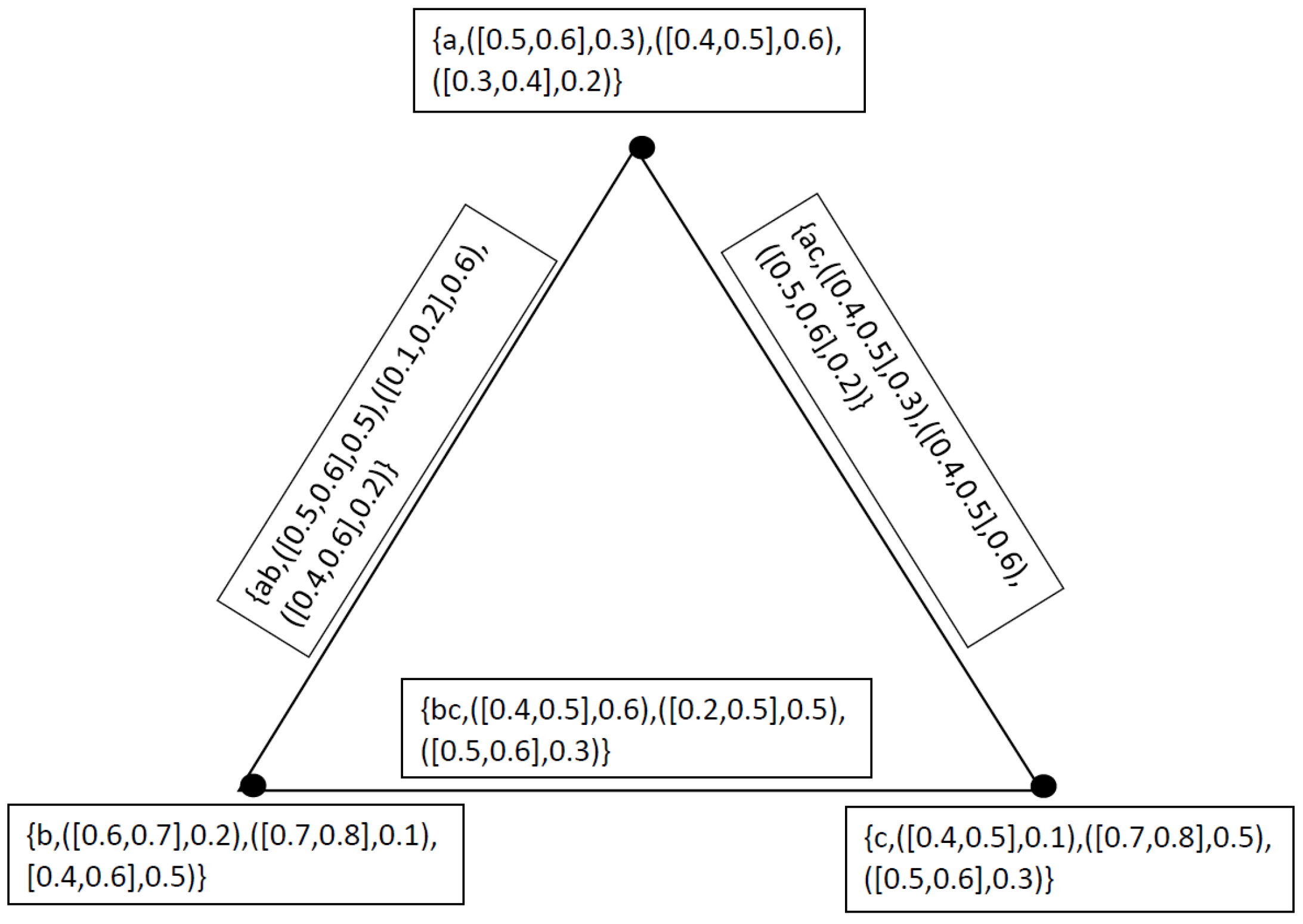
Example 1.
Let be a graph where and , where
Then clearly is a neutrosophic cubic graph of as showin in Figure 1.
Remark 1.
- 1.
- If in the vertex set and in the set of edges then the graphs is a neutrosophic cubic polygon only when we join each vertex to the corresponding vertex through an edge.
- 2.
- If we have infinite elements in the vertex set and by joining the each and every edge with each other we get a neutrosophic cubic curve.
Definition 10.
Let be a neutrosophic cubic graph. The order of neutrosophic cubic graph is defined by and degree of a vertex x in G is defined by .
Example 2.
In Example 1, Order of a neutrosophic cubic graph is
and degree of each vertex in G is
Definition 11.
Let be a neutrosophic cubic graph of and be a neutrosophic cubic graph of . Then Cartesian product of and is denoted by
and is defined as follow
- (i)
- (ii)
- (iii)
- (iv)
- (v)
- (vi)
- (vii)
- (viii)
- (ix)
- ∀ for and for and for .
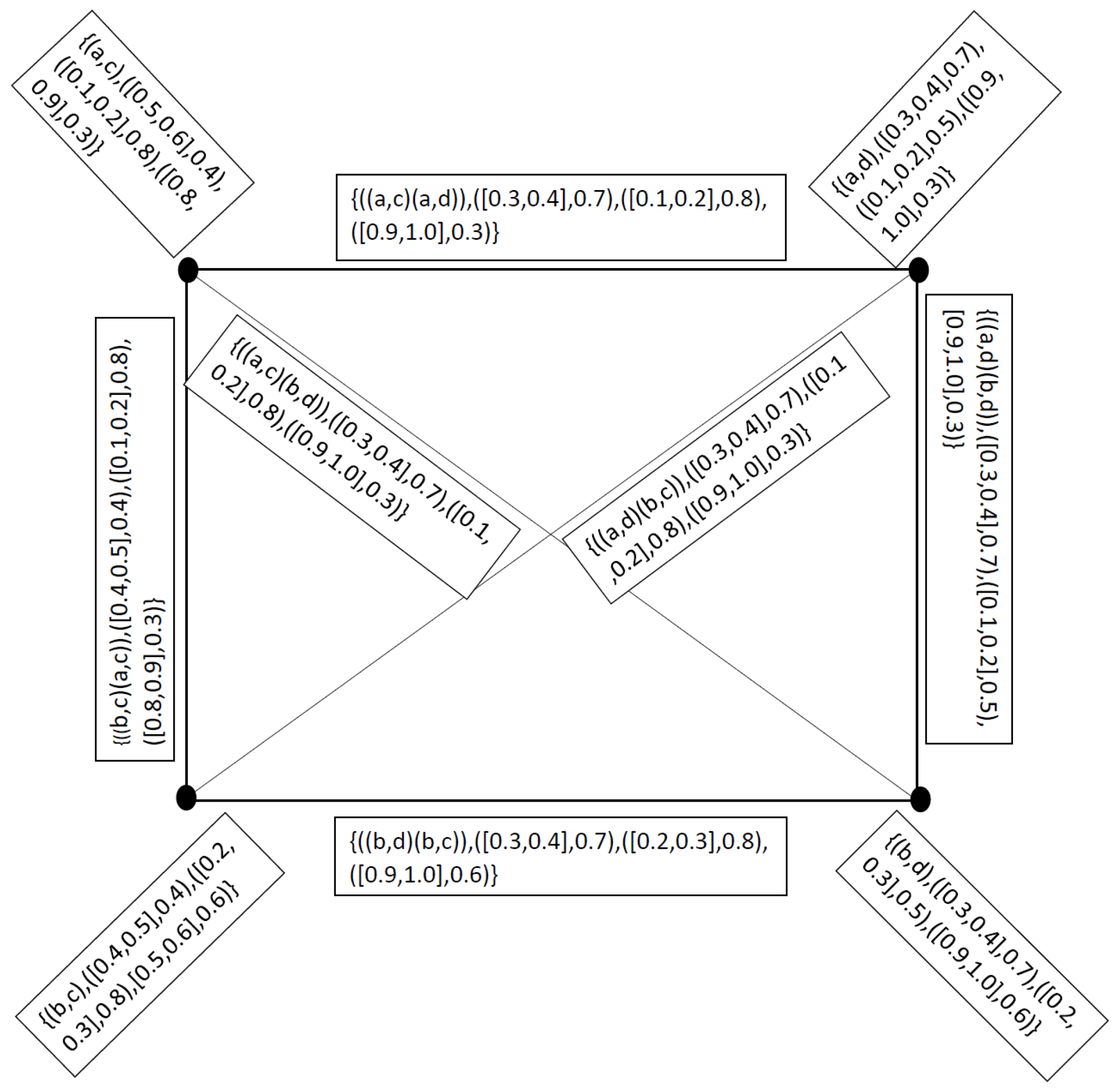
Example 3.
Proposition 1.
The cartesian product of two neutrosophic cubic graphs is again a neutrosophic cubic graph.
Proof.
Condition is obvious for . Therefore we verify conditions only for where Let and . Then
similarly we can prove it for and . ☐
Definition 12.
Let and be two neutrosophic cubic graphs. The degree of a vertex in can be defined as follows, for any
Example 4.
In Example 3
Definition 13.
Let be a neutrosophic cubic graph of and be a neutrosophic cubic graph of Then composition of and is denoted by and defined as follow
where
- (i)
- (ii)
- and
- (iii)
- and
- (iv)
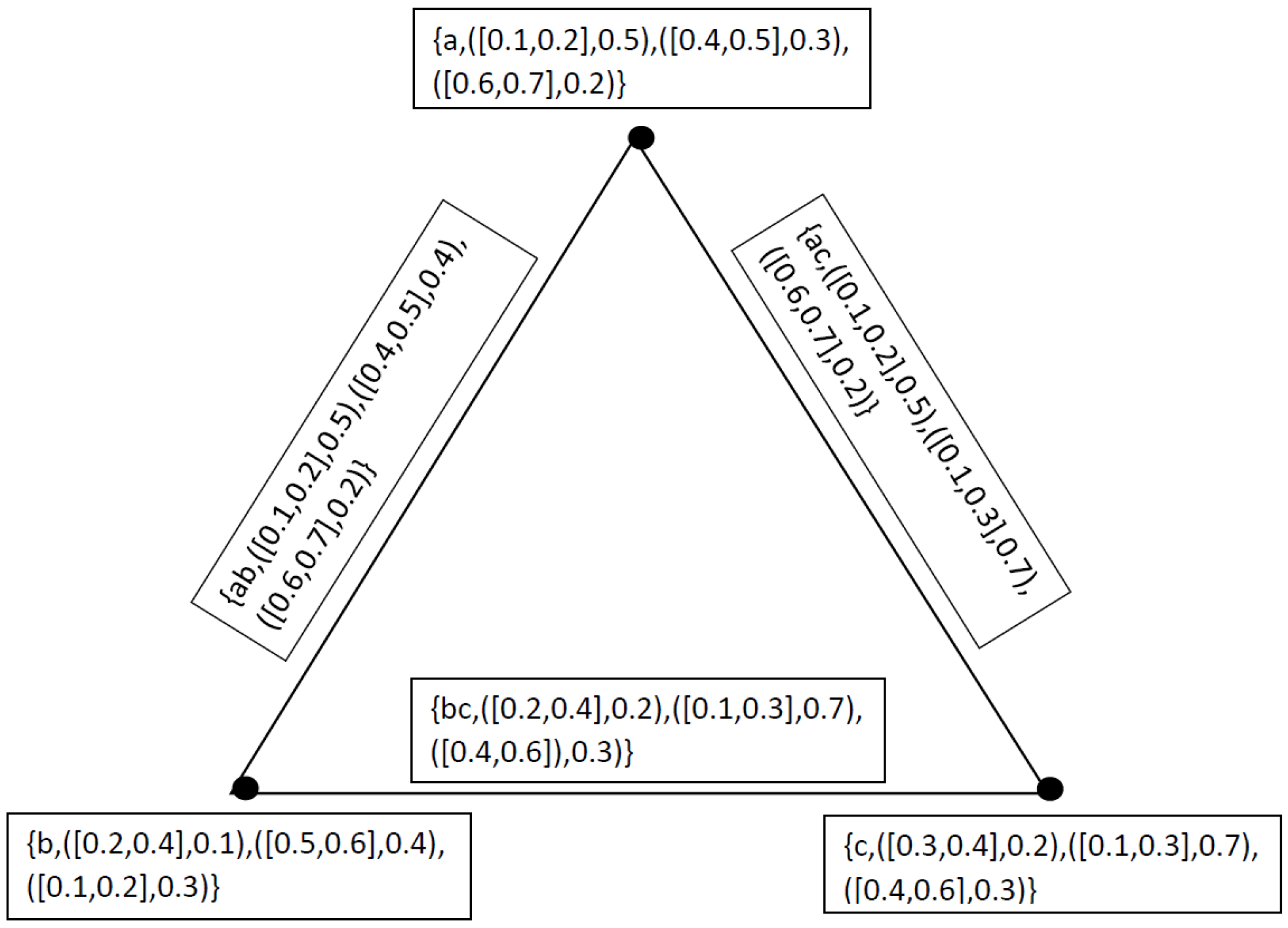
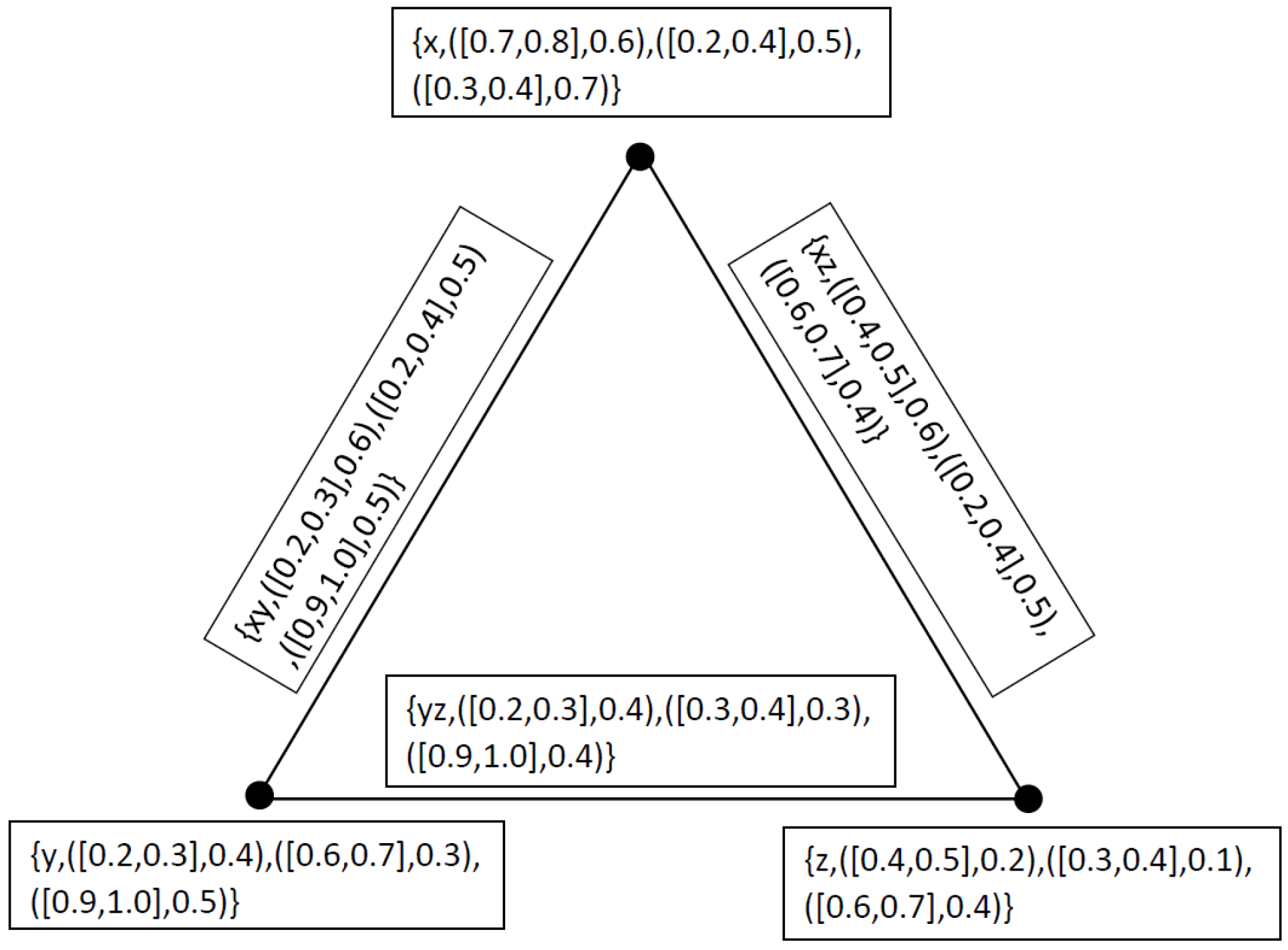
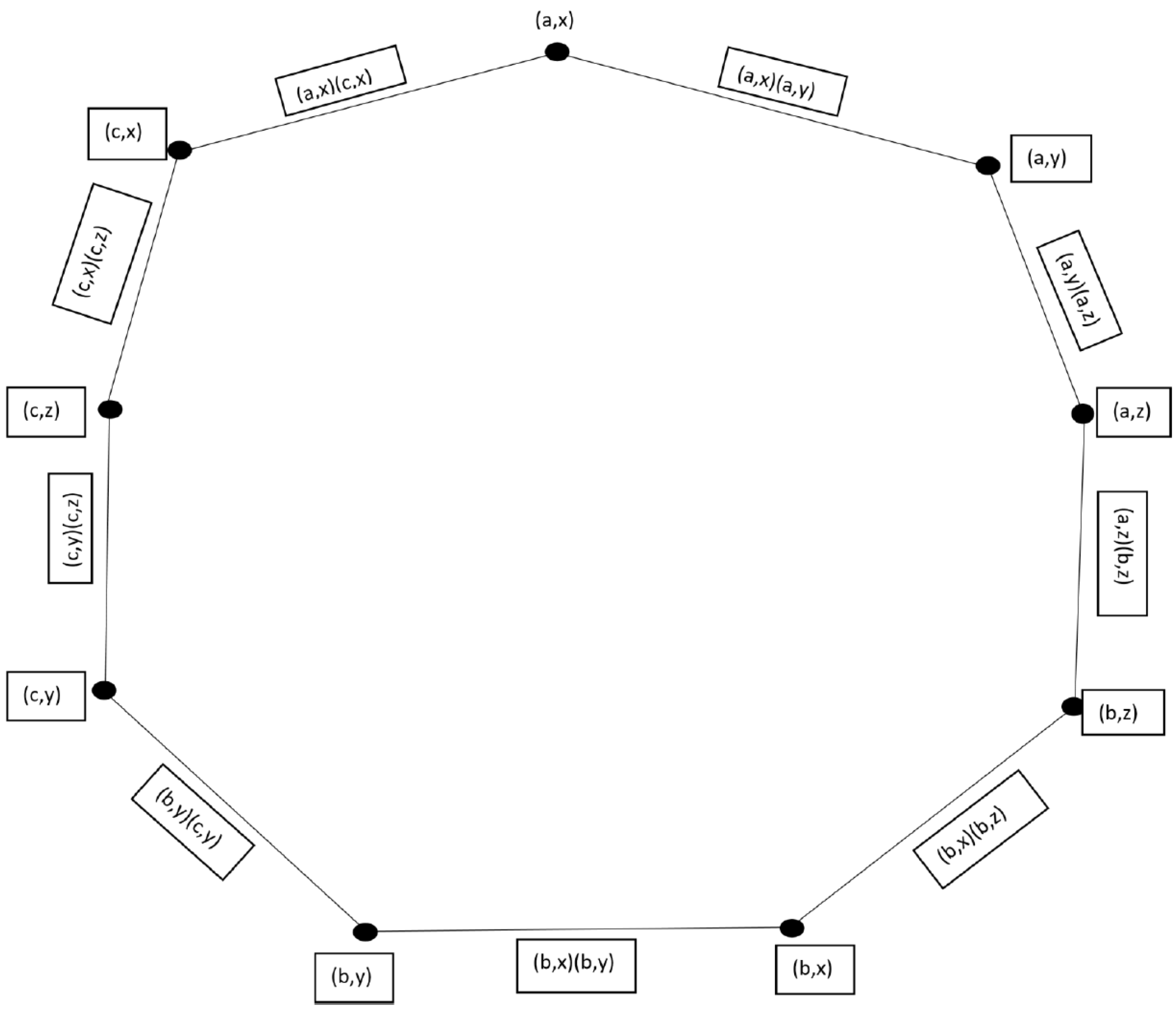
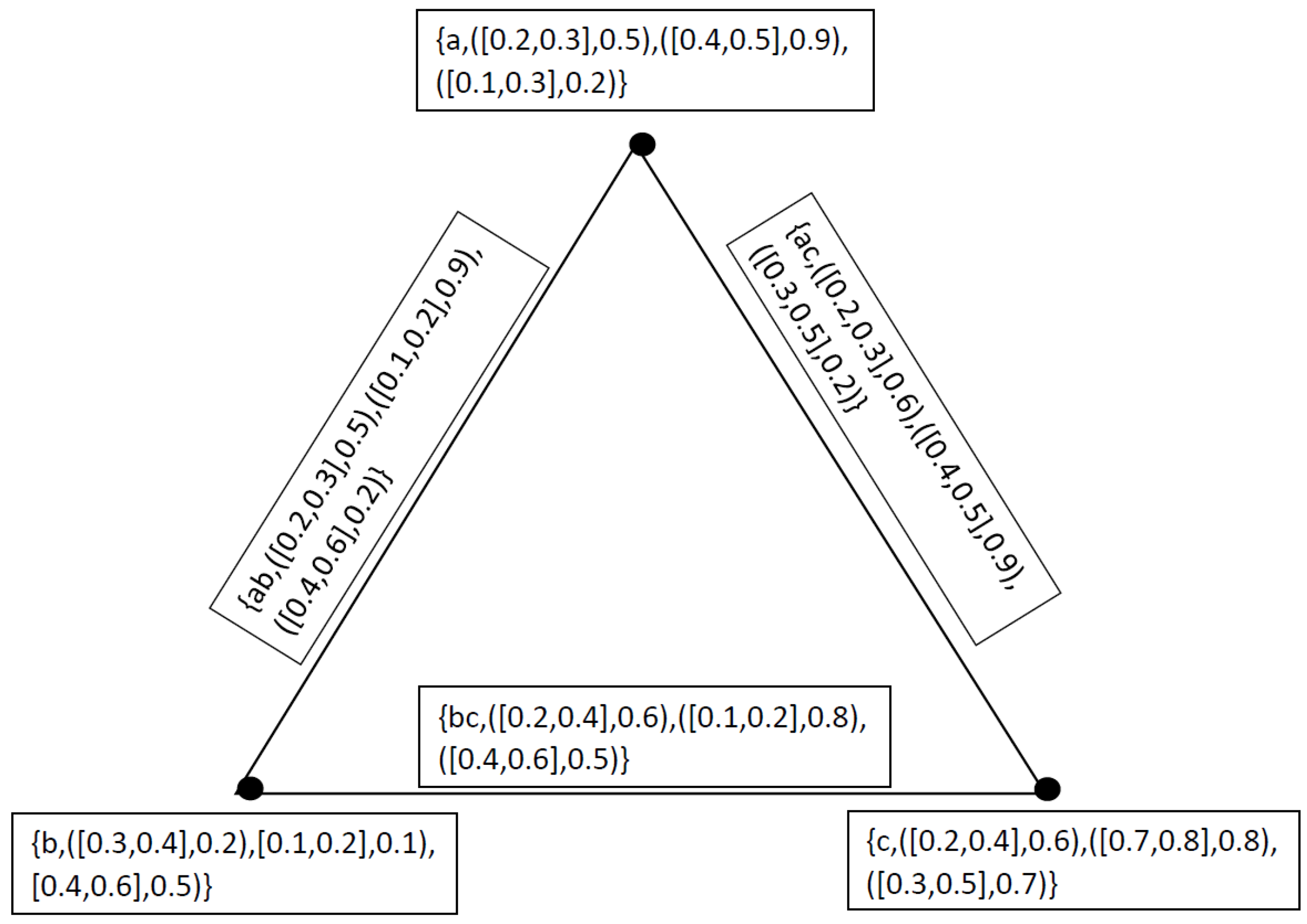
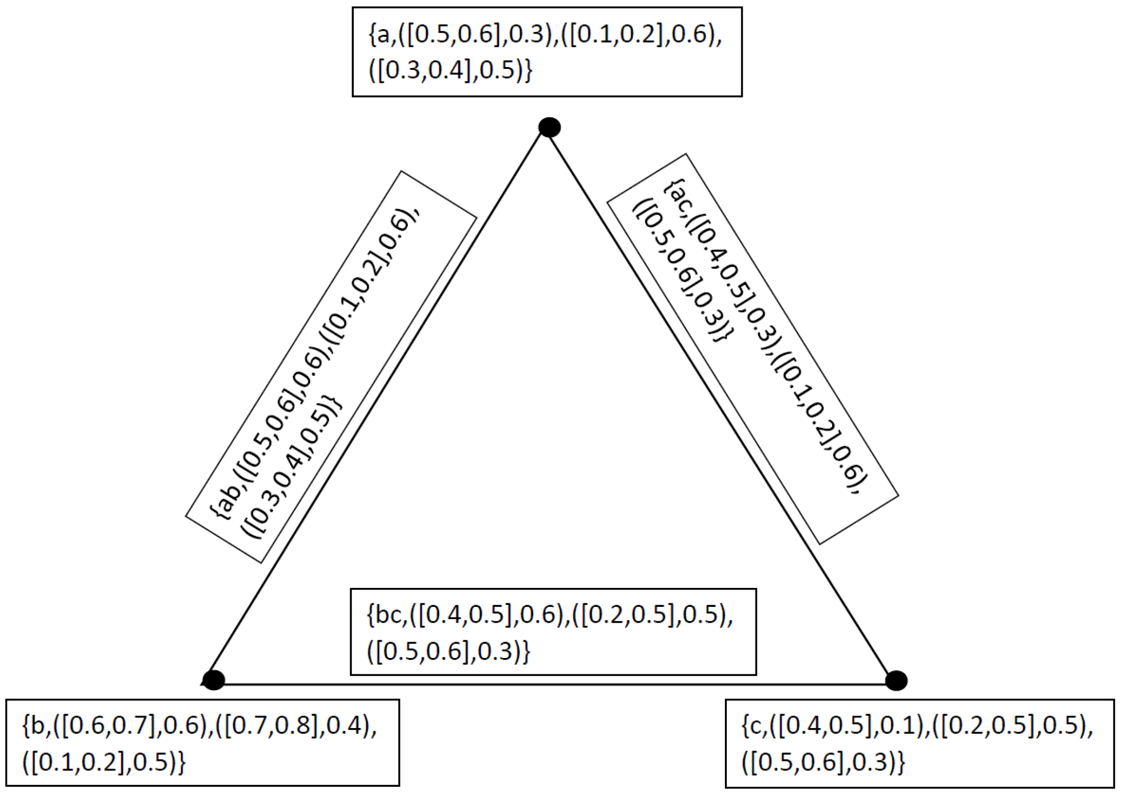
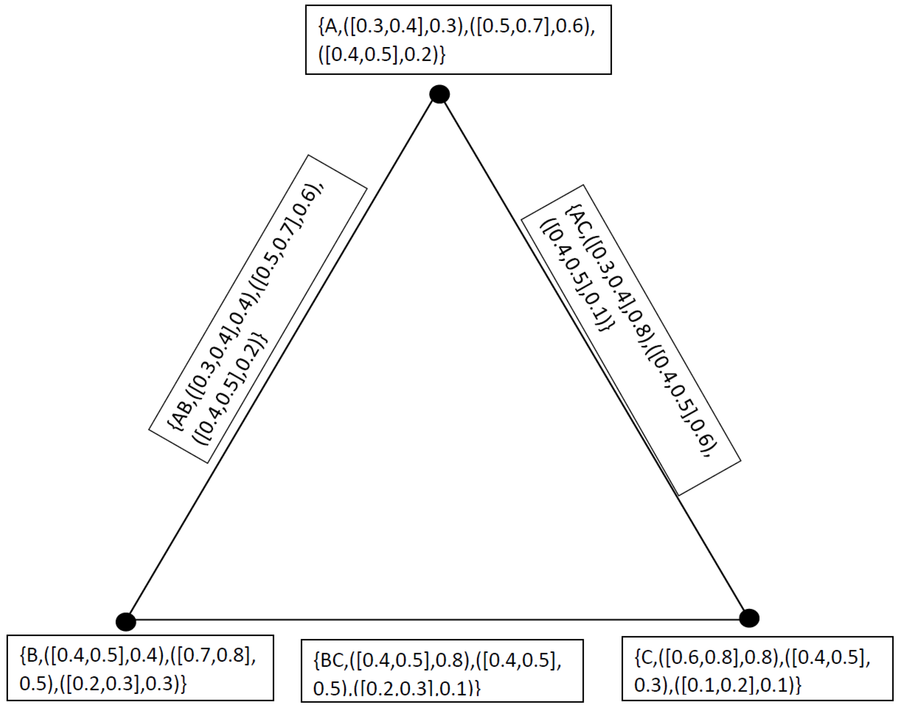
Example 5.
Let and be two graphs as showin in Figure 5, where and . Suppose and be the neutrosophic cubic set representations of and Also and be the neutrosophic cubic set representations of and defined as
and
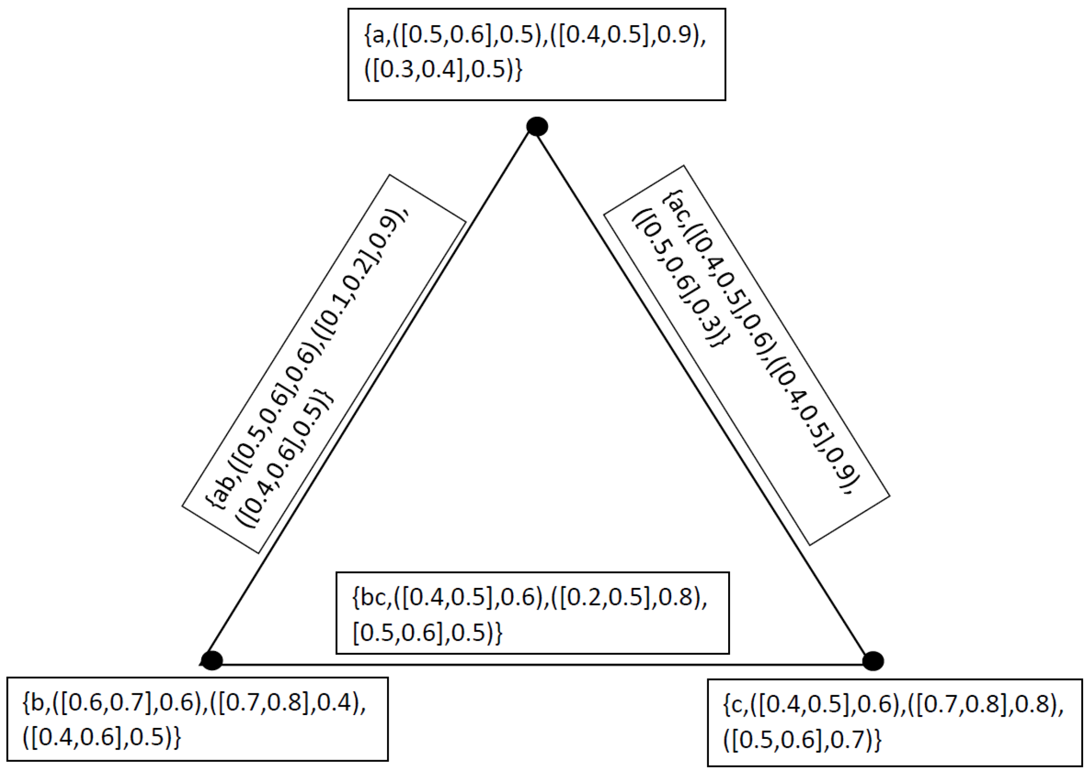
Clearly and are neutrosophic cubic graphs. So, the composition of two neutrosophic cubic graphs and is again a neutrosophic cubic graph as shown in Figure 6, where
Proposition 2.
The composition of two neutrosophic cubic graphs is again a neutrosophic cubic graph.
Definition 14.
Let and be two neutrosophic cubic graphs of the graphs and respectively. Then P-union is denoted by and is defined as
where
and R-union is denoted by and is defined by
where
Example 6.
Proposition 3.
The P-union of two neutrosophic cubic graphs is again a neutrosophic cubic graph.
Remark 2.
The R-union of two neutrosophic cubic graphs may or may not be a neutrosophic cubic graph as in the Example 6 we see that
Definition 15.
Let and be two neutrosophic cubic graphs of the graphs and respectively then P-join is denoted by and is defined by
where
- (i)
- if
- (ii)
- if
- (iii)
- if , where is the set of all edges joining the vertices of and
Definition 16.
Let and be two neutrosophic cubic graphs of the graphs and respectively then R-join is denoted by and is defined by
where
- (i)
- if
- (ii)
- if
- (iii)
- if , where is the set of all edges joining the vertices of and
Proposition 4.
The P-join and R-join of two neutrosophic cubic graphs is again a neutrosophic cubic graph.
4. Applications
Fuzzy graph theory is an effective field having a vast range of applications in Mathematics. Neutrosophic cubic graphs are more general and effective approach used in daily life very effectively.
Here in this section we test the applicability of our proposed model by providing applications in industries.
Example 7.
Let us suppose a set of three industries representing a vertex set and let the truth-membership of each vertex in V denotes “win win” situation of industry, where they do not harm each other and do not capture other’s customers. Indetermined-membership of members of vertex set represents the situation in which industry works in a diplomatic and social way, that is, they are ally being social and competitive being industry. Falsity-membership shows a brutal competition where price war starts among industries. We want to observe the effect of one industry on other industry with respect to their business power and strategies. Let we have a neutrosophic cubic graph for industries having the following data with respect to business strategies
where interval memberships indicate the business strength and strategies of industries for the present time while fixed membership indicates the business strength and strategies of industries for future based on given information. So on the basis of M we get a set of edges defined as
where interval memberships indicate the business strength and strategies of industries for the present time while fixed membership indicate the business strength and strategies of industries for future when it will be the time of more competition. It is represented in Figure 11.
Finally we see that the business strategies of one industry strongly affect its business with other industries. Here
and
Order of G represents the overall effect on market of above given industries A, B and C. Degree of A represents the effect of other industries on A link through an edge with the industry A. The minimum degree of A is 0 when it has no link with any other.
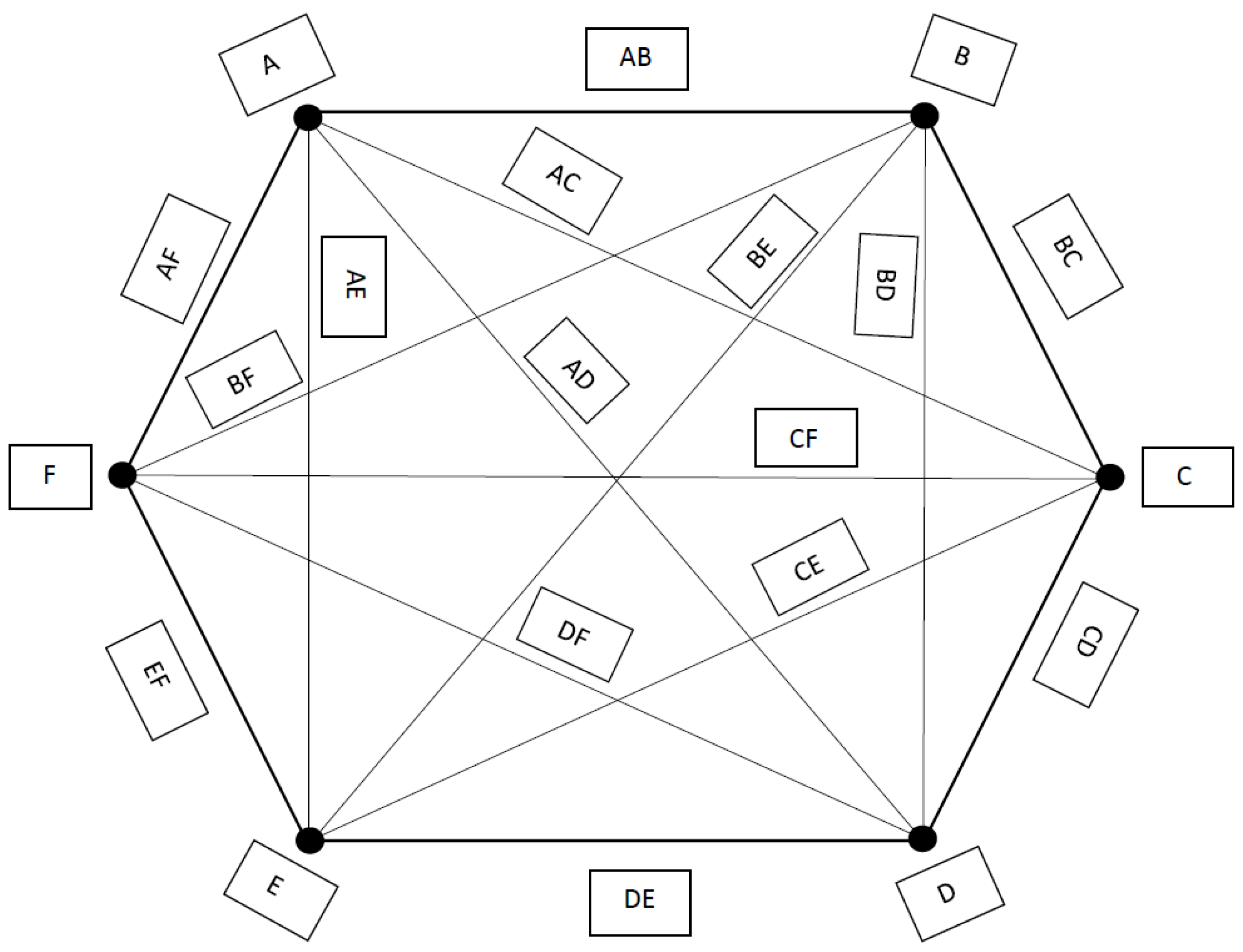
Example 8.
Let us take an industry and we want to evaluate its overall performance. There are a lot of factors affecting it. However, some of the important factors influencing industrial productivity are with neutrosophic cubic sets as under, where the data is provided in the form of interval based on future prediction and data given in the form of a number from the unit interval is dependent on the present time after a careful testing of different models as a sample in each case,
- 1.
- Technological Development degree of mechanization), (technical know-how), (product design
- 2.
- Quality of Human Resources ability of the worker), (willingness of the worker), (the environment under which he has to work
- 3.
- Availability of Finance advertisement campaign), (better working conditions to the workers), (up-keep of plant and machinery,
- 4.
- Managerial Talent devoted towards their profession), (Links with workers, customers and suppliers), (conceptual, human relations and technical skills
- 5.
- Government Policy Government Policy favorable conditions for saving), (investment), (flow of capital from one industrial sector to another
- 6.
- Natural Factors physical), (geographical(climatic exercise. As these factors affecting industrial productivity are inter-related and inter-dependent, it is a difficult task to evaluate the influence of each individual factor on the overall productivity of industrial units. The use of neutrosophic cubic graphs give us a more reliable information as under. Let we have a neutrosophic cubic set for the vertex set as under
Now, in order to find the combined effect of all these factors we need to use neutrosophic cubic sets for edges as under
where the edge denotes the combined effect of technological development and quality of human resources on the productivity of the industry. Now, if we are interested to find which factors are more effective to the productivity of the industry, we may use the score and accuracy of the neutrosophic cubic sets, which will give us a closer view of the factors. It is represented in Figure 12.
Remark. We used degree and order of the neutrosophic cubic graphs in an application see Example 7 and if we have two different sets of industries having finite number of elements, we can easily find the applications of cartesian product, composition, union, join, order and degree of neutrosophic cubic graphs.
5. Comparison Analysis
In 1975, Rosenfeld discussed the concept of fuzzy graphs whose basic idea was introduced by [3] Kauffmann in 1973. Atanassov extended this idea to intuitionistic fuzzy graphs [14] in 1995. The idea of neutrosophic graphs provided by Kandasamy et al. in the book [29]. [38] Recently Rashid et al., introduced the notion of cubic graphs. In this paper, we introduced the study of neutrosophic cubic graphs. We claim that our model is more generalized from the previous models, as if we both indeterminacy and falsity part of neutrosophic cubic graphs where is the neutrosophic cubic set representation of vertex set V and is the neutrosophic cubic set representation of edges set E vanishes we get a cubic graph provided by Rashid et al., in [38]. Similarly, by imposing certain conditions on cubic graphs, we may obtain intuitionistic fuzzy graphs provided by Atanassov in 1995 and after that fuzzy graphs provided by Rosenfeld in 1975. So our proposed model is a generalized model and it has the ability to capture the uncertainty in a better way.
6. Conclusions
A generalization of the old concepts is the main motive of research. So in this paper, we proposed a generalized model of neutrosophic cubic graphs with different binary operations. We also provided applications of neutrosophic cubic graphs in industries. We also discussed conditions under which our model reduces to the previous models. In future, we will try to discuss different types of neutrosophic cubic graphs such as internal neutrosophic cubic graphs, external neutrosophic cubic graphs and many more with applications.
Author Contributions
Write up Z.R., Methodology, N.Y.; Project administration, F.S.; Supervision, M.G.; English Editing, H.A.W.
Conflicts of Interest
The authors declare no conflict of interest.
References
- Zadeh, L.A. Fuzzy sets. Inf. Control 1965, 8, 338–353. [Google Scholar]
- Rosenfeld, A. Fuzzy Graphs, Fuzzy Sets and Their Applications; Academic Press: New York, NY, USA, 1975; pp. 77–95. [Google Scholar]
- Kauffman, A. Introduction a la Theorie des Sous-Emsembles Flous; Masson: Issy-les-Moulineaux, French, 1973; Volume 1. [Google Scholar]
- Bhattacharya, P. Some remarks on fuzzy graphs. Pattern Recognit. Lett. 1987, 6, 297–302. [Google Scholar]
- Akram, M.; Dudek, W.A. Interval-valued fuzzy graphs. Comput. Math. Appl. 2011, 61, 289–299. [Google Scholar] [Green Version]
- Akram, M. Interval-valued fuzzy line graphs. Neural Comput. Appl. 2012, 21, 145–150. [Google Scholar]
- Mordeson, J.N.; Nair, P.S. Fuzzy Graphs and Fuzzy Hypergraphs; Springer: Berlin/Heidelberg, Germany, 2001. [Google Scholar]
- Sunitha, M.S.; Sameena, K. Characterization of g-self centered fuzzy graphs. J. Fuzzy Math. 2008, 16, 787–791. [Google Scholar]
- Borzooei, R.A.; Rashmanlou, H. Cayley interval-valued fuzzy threshold graphs, U.P.B. Sci. Bull. Ser. A 2016, 78, 83–94. [Google Scholar]
- Pal, M.; Samanta, S.; Rashmanlou, H. Some results on interval-valued fuzzy graphs. Int. J. Comput. Sci. Electron. Eng. 2015, 3, 2320–4028. [Google Scholar]
- Pramanik, T.; Pal, M.; Mondal, S. Inteval-valued fuzzy threshold graph. Pac. Sci. Rev. A Nat. Sci. Eng. 2016, 18, 66–71. [Google Scholar]
- Pramanik, T.; Samanta, S.; Pal, M. Interval-valued fuzzy planar graphs. Int. J. Mach. Learn. Cybern. 2016, 7, 653–664. [Google Scholar]
- Atanassov, K.T. Intuitionistic fuzzy sets. Fuzzy Sets Syst. 1986, 20, 87–96. [Google Scholar]
- Atanassov, K.T. On Intuitionistic Fuzzy Graphs and Intuitionistic Fuzzy Relations. In Proceedings of the VI IFSA World Congress, Sao Paulo, Brazil, 22–28 July 1995; Volume 1, pp. 551–554. [Google Scholar]
- Atanassov, K.T.; Shannon, A. On a generalization of intuitionistic fuzzy graphs. Notes Intuit. Fuzzy Sets 2006, 12, 24–29. [Google Scholar]
- Karunambigai, M.G.; Parvathi, R. Intuitionistic Fuzzy Graphs. In Computational Intelligence, Theory and Applications; Springer: Berlin/Heidelberg, Germany, 2006; Volume 20, pp. 139–150. [Google Scholar]
- Shannon, A.; Atanassov, K.T. A first step to a theory of the intutionistic fuzzy graphs. In Proceedings of the 1st Workshop on Fuzzy Based Expert Systems, Sofia, Bulgaria, 26–29 June 1994; pp. 59–61. [Google Scholar]
- Mishra, S.N.; Rashmanlou, H.; Pal, A. Coherent category of interval-valued intuitionistic fuzzy graphs. J. Mult. Val. Log. Soft Comput. 2017, 29, 355–372. [Google Scholar]
- Parvathi, R.; Karunambigai, M.G.; Atanassov, K. Operations on Intuitionistic Fuzzy Graphs. In Proceedings of the IEEE International Conference on Fuzzy Systems, Jeju Island, Korea, 20–24 August 2009; pp. 1396–1401. [Google Scholar]
- Sahoo, S.; Pal, M. Product of intiutionistic fuzzy graphs and degree. J. Intell. Fuzzy Syst. 2017, 32, 1059–1067. [Google Scholar]
- Akram, M.; Davvaz, B. Strong intuitionistic fuzzy graphs. Filomat 2012, 26, 177–196. [Google Scholar]
- Zhang, W.R. Bipolar Fuzzy Sets and Relations: A Computational Framework for Coginitive Modeling and Multiagent Decision Analysis. In Proceedings of the IEEE Industrial Fuzzy Control and Intelligent Systems Conference, and the NASA Joint Technology Workshop on Neural Networks and Fuzzy Logic, Fuzzy Information Processing Society Biannual Conference, San Antonio, TX, USA, 18–21 December 1994; pp. 305–309. [Google Scholar]
- Akram, M. Bipolar fuzzy graphs. Inf. Sci. 2011, 181, 5548–5564. [Google Scholar]
- Akram, M. Bipolar fuzzy graphs with applications. Knowl. Based Syst. 2013, 39, 1–8. [Google Scholar]
- Akram, M.; Karunambigai, M.G. Metric in bipolar fuzzy graphs. World Appl. Sci. J. 2012, 14, 1920–1927. [Google Scholar]
- Smarandache, F. A Unifying Field in Logics: Neutrosophic Logic. Neutrosophy, Neutrosophic Set, Neutrosophic Probability; American Research Press: Rehoboth, NM, USA, 1999. [Google Scholar]
- Smarandache, F. Neutrosophic set-a generalization of the intuitionistic fuzzy set. Int. J. Pure Appl. Math. 2005, 24, 287–297. [Google Scholar]
- Wang, H.; Smarandache, F.; Zhang, Y.Q.; Sunderraman, R. Interval Neutrosophic Sets and Logic: Theory nd Applications in Computing; Hexis: phoenix, AZ, USA, 2005. [Google Scholar]
- Kandasamy, W.B.V.; Ilanthenral, K.; Smarandache, F. Neutrosophic Graphs: A New Dimension to Graph Theory; EuropaNova ASBL: Bruxelles, Belgium, 2015. [Google Scholar]
- Akram, M.; Rafique, S.; Davvaz, B. New concepts in neutrosophic graphs with application. J. Appl. Math. Comput. 2018, 57, 279–302. [Google Scholar]
- Akram, M.; Nasir, M. Concepts of Interval-Valued Neutrosophic Graphs. Int. J. Algebra Stat. 2017, 6, 22–41. [Google Scholar]
- Akram, M. Single-valued neutrosophic planar graphs. Int. J. Algebra Stat. 2016, 5, 157–167. [Google Scholar]
- Akram, M.; Shahzadi, S. Neutrosophic soft graphs with application. J. Intell. Fuzzy Syst. 2017, 32, 841–858. [Google Scholar]
- Jun, Y.B.; Kim, C.S.; Yang, K.O. Cubic Sets. Ann. Fuzzy Math. Inf. 2012, 4, 83–98. [Google Scholar]
- Jun, Y.B.; Kim, C.S.; Kang, M.S. Cubic subalgebras and ideals of BCK/BCI-algebras. Far East J. Math. Sci. 2010, 44, 239–250. [Google Scholar]
- Jun, Y.B.; Lee, K.J.; Kang, M.S. Cubic structures applied to ideals of BCI-algebras. Comput. Math. Appl. 2011, 62, 3334–3342. [Google Scholar]
- Kang, J.G.; Kim, C.S. Mappings of cubic sets. Commun. Commun. Korean Math. Soc. 2016, 31, 423–431. [Google Scholar]
- Rashid, S.; Yaqoob, N.; Akram, M.; Gulistan, M. Cubic Graphs with Application. Int. J. Anal. Appl. 2018, in press. [Google Scholar]
- Jun, Y.B.; Smarandache, F.; Kim, C.S. Neutrosophic cubic sets. New Math. Nat. Comput. 2017, 13, 41–54. [Google Scholar]
- Jun, Y.B.; Smarandache, F.; Kim, C.S. P-union and P-intersection of neutrosophic cubic sets. Anal. Univ. Ovid. Constant. Seria Mat. 2017, 25, 99–115. [Google Scholar] [Green Version]
Figure 1.
Neutrosophic Cubic Graph.

Figure 2.
Neutrosophic Cubic Graph .

Figure 3.
Neutrosophic Cubic Graph .

Figure 4.
Cartesian Product of and .

Figure 5.
Neutrosophic Cubic Graph and .
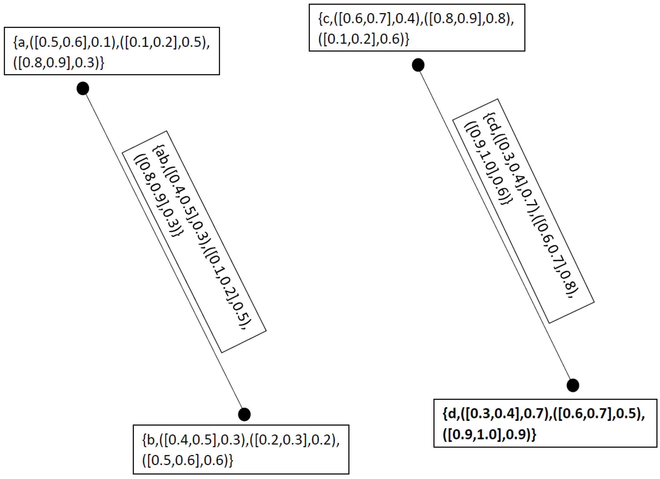
Figure 6.
Composition of and .

Figure 7.
Neutrosophic Cubic Graph .

Figure 8.
Neutrosophic Cubic Graph .

Figure 9.
P-Union of and .

Figure 10.
R-Union of and .

Figure 11.
Neutrosophic Cubic Graph.

Figure 12.
Neutrosophic Cubic Graph.
© 2018 by the authors. Licensee MDPI, Basel, Switzerland. This article is an open access article distributed under the terms and conditions of the Creative Commons Attribution (CC BY) license (http://creativecommons.org/licenses/by/4.0/).
Share and Cite
MDPI and ACS Style
Gulistan, M.; Yaqoob, N.; Rashid, Z.; Smarandache, F.; Wahab, H.A. A Study on Neutrosophic Cubic Graphs with Real Life Applications in Industries. Symmetry 2018, 10, 203. https://doi.org/10.3390/sym10060203
AMA Style
Gulistan M, Yaqoob N, Rashid Z, Smarandache F, Wahab HA. A Study on Neutrosophic Cubic Graphs with Real Life Applications in Industries. Symmetry. 2018; 10(6):203. https://doi.org/10.3390/sym10060203
Chicago/Turabian StyleGulistan, Muhammad, Naveed Yaqoob, Zunaira Rashid, Florentin Smarandache, and Hafiz Abdul Wahab. 2018. "A Study on Neutrosophic Cubic Graphs with Real Life Applications in Industries" Symmetry 10, no. 6: 203. https://doi.org/10.3390/sym10060203
Note that from the first issue of 2016, this journal uses article numbers instead of page numbers. See further details here.