An Improved Whale Optimization Algorithm Based on Different Searching Paths and Perceptual Disturbance

Abstract

Whale optimization algorithm (WOA) is a swarm intelligence optimization algorithm inspired by humpback whale hunting behavior. WOA has many similarities with other swarm intelligence algorithms (PSO, GWO, etc.). WOA’s unique search mechanism enables it to have a strong global search capability while taking into account the strong global search capabilities. In this work, considering the the deficiency of WOA in local search mechanism, combined with the optimization methods of other group intelligent algorithms, perceptual perturbation mechanism is introduced, which makes the agent perform more detailed searches near the local extreme point. At the same time, since the WOA uses a logarithmic spiral curve, the agent cannot fully search all the spaces within its search range, even though the introduction of the perturbation mechanism may still lead to the algorithm falling into a local optimum. Therefore, the equal pitch Archimedes spiral curve is chosen to replace the classic logarithmic spiral curve. In order to fully verify the effect of the search path on the performance of the algorithm, several other spiral curves have been chosen for experimental comparison. By utilizing the 23 benchmark test functions, the simulation results show that WOA (PDWOA) with perceptual perturbation significantly outperforms the standard WOA. Then, based on the PDWOA, the effect of the search path on the performance of the algorithm has been verified. The simulation results show that the equal pitch of the Archimedean spiral curve is best.

1. Introduction

Problems with optimization must find the most optimal solution of the objective function by iteration. Generally, the search target—which can be described by coutinuous, descrete, linear, unlinear, convace, and convex functions—is a function that belongs to optimal objective functions. In order to solve the problem of function optimization, a heuristic algorithm inspired by natural processes and/or events has raised concerns. Swarm intelligence optimization algorithms that simulate biological population evolution is a random search algorithm. It can solve complex global optimization problems through cooperation and competition among individuals. Swarm intelligence optimization algorithm include the ant colony optimization (ACO) algorithm [1,2,3], genetic algorithm (GA) [4,5], particle swarm optimization (PSO) algorithm [6,7,8], artificial bee colony (ABC) algorithm [9], grey wolf algorithm (GWO) [10], harmony search (HS) Algorithm [11,12], etc.

The whale optimization algorithm (WOA) is a biological heuristic algorithm presented by Seyedali Mirjalili and Andrew Lewis in 2016. WOA is a swarm intelligence optimization algorithm inspired by the unique humpback hunting method. Because of unique optimization mechanism, WOA has a good global search capability. Therefore, the new algorithm has been widely proposed by the engineering community. As a new type of bionic algorithm with better global search performance, many scholars are interested in it and apply it to a variety of engineering problems. It has been widely used in the optimization of neural network parameters, allocation, and scheduling. On the allocation and scheduling, the literatures [13,14,15,16] use WOA to optimize energy management system (EMS) of the Combined Economic Emission Dispatch (CEED) problem for microgrid systems, and MATLAB software is used to compared it with GM, ACO, PSO and WOA; the results show that WOA can obtain better results with fewer iterations. The literature [17] applies WOA to the Unit Commitment Problem of power generation operation scheduling, the experimental results show that the convergence speed of WOA is obviously faster than PSO, GA, etc. In order to reduce the wire loss of distribution network, the literature [18] uses WOA to optimize the distribution scheme of the capacitors in the grid. The simulation results show that WOA is more effective in reducing operating costs and maintaining better voltage distribution. Similarly, the literature [19] uses the WOA to the water resources scheduling problem. The research results show that WOA has a faster convergence speed.

In terms of parameter optimization, the literature [20] uses WOA to optimize two parameters of a least-squares support vector machine to establish a WOA-LSSVM (WOA-least-squares support vector machine) model to predict carbon dioxide emissions. Similarly, chaos WOA algorithm (CWOA) is proposed to optimize the parameters of Elman neural network in the literature [21], so as to establish a soft measurement model and predict variables. The literature [22] compares WOA with other methods for optimizing neural network parameters quantitatively and qualitatively. Simulation results show that the proposed trainer can outperform current algorithms on most data sets in terms of local optimal avoidance and convergence speed. The literature [23] uses WOA to optimize the parameters of the multilayer perception model, and it uses five standard data sets to verify the validity of the modified model. We compared it with GWO and PSO, and found a high convergence and classification rate of WOA, and it is possible to avoid local minimums.

In terms of variable prediction, the literature [24] proposes a multi-objective whale optimization algorithm (MOWOA) model to predict the wind speed in the power system and thus provide a reference for power dispatching. The literature [25] combines the reverse adaptive whale optimization algorithm (AWOA) and the fast learning network (FLN) to propose an integrated modeling method (AWOA-FLN) and establishes a 600-MW prediction model for supercritical steam turbine group heat rate. Simulation results show that the AWOA-FLN model has stronger prediction accuracy and stronger generalization ability than the improved PSO algorithm and differential evolution algorithm, and it can more accurate predict the heat rate of the turbine. In image processing, in order to find the best image segmentation threshold, the literature [26] combines WOA and moth-flame optimization to avoid the problem of determining the optimal threshold spend too much time in the case of multilevel thresholds. The simulation results show that the proposed algorithm has better performance than other swarm intelligence algorithms. The literature [27] propose a MRI image liver segmentation method based on the whale optimization algorithm (WOA). The proposed method uses a set of 70 magnetic resonance images (MRI) images for testing. The experimental results show that the method has a high accuracy overall. In addition, considering WOA optimization and other applications, the literature [28] introduces the nondominated sorting algorithm to obtain the optimal solution of WOA, named the nondominated sorting WOA (NSWOA). The simulation results show that the method is much better than multiobjective collision-body optimizer (MOCBO), multi-objective particle swarm optimizer (MOPSO), nondominated sorting genetic algorithm II (NSGA-II) and the multiobjective symbiotic organism search (MOSOS). The literature [29] proposed a chaos WOA (CWOA) algorithm to calculate and automatically adjust the internal parameters of the optimization algorithm through chaotic mapping. This idea is essentially different from the literature [21]. The experimental results show that CWOA can effectively optimize the parameters of photovoltaic cells and their components. The literature [30] proposes a WOA-based feature selection approach, which is applied to find the largest subset of features so that it maximizes classification accuracy while retaining the minimum number of features.

The essence of a group intelligence algorithm is to find the global optimal value as much as possible with the help of various mechanisms. The improvement ideas proposed by many scholars are as far as possible to complete the search mechanism of group intelligent algorithm, so that the search agent traverses the entire search space as much as possible.

In this paper, we analyze the search mechanism of the WOA algorithm and find that its search mechanism has defects. However, this kind of defect cannot be solved by adjusting the moving step length. The original WOA uses a logarithmic spiral curve as the search path of the agent. However, the screw pitch of the logarithmic spiral curve is not fixed. Because the screw pitch causes a large amount of agent movements in the early stage, some areas cannot be searched. As a result, the global optimum is ignored. For this problem, this paper proposes a WOA with perceptual perturbation [31,32,33] so that the agent can perturb near the local extreme points to obtain better optimal values as much as possible. The closest to the idea of this paper is the literature [34]. In order to improve the PSO’s local search ability, literature [34] defines and analyzes the regions with the most particles. At the same time, presented a PSO algorithm with intermediate disturbance searching strategy (IDPSO), which enhances the global search ability of particles and increases their convergence rates. Introducing the perturbation mechanism into the group intelligent algorithm can effectively improve the performance of the algorithm. The difference between this article and other methods is that the step length is set to make the search agent’s moving step smaller and smaller, so that the agent can search more and more carefully. The definition of the minimum step size makes it impossible for the agent’s step size to be smaller and smaller, thus ensuring the algorithm’s convergence speed and ability to jump out of the local extreme point. At the same time, for the defects of the search mechanism, this paper uses the remaining seven spiral curves instead of the original logarithmic spiral curve to obtain an optimal search path. Finally, we select 23 benchmark test functions to verify the effectiveness of perceived perturbation and remaining spiral curves.

The structure of this paper is as follows: we have an introduction in the first section. The second section introduces the WOA optimization algorithm and analyzes the defects of the algorithm. The third section introduces the idea and method of improving WOA. The fourth section is a simulation, and a summary in the fifth section.

2. Whale Optimization Algorithm

2.1. Inspiration

The whale optimization algorithm (WOA) is inspired by the unique hunting method of the humpback whale, which is called the bubble-net predation method [35,36,37,38,39]. The humpback whale can perceive the distance between him and the prey and surround the prey. It is observed that the humpback whale can move up with a spiral path in about 15 m deep, and spit out a number of different sizes of bubbles. The last spit out bubble and the first spit out bubble rose to the surface at the same time so as to form a cylindrical or tubular bubble network. It likes a huge spider knotted web to surround the prey tightly, and makes the prey toward the center of the net. So the humpback whales almost upright open mouth in the bubble circle and swallow the prey in the net. According to the above descriptions, the hunting behavior of the humpback whale can be divided into three steps: encircling prey, spiral bubble-net feeding maneuver and searching for prey.

2.2. Search for Prey (Exploration Phase)

In order to establish the mathematical model of the humpback whale searching path, each humpback whale is set as a search agent. At the same time, the algorithm is divided into three steps: the search for prey, encircling prey and spiral bubble-net attacking method (exploitation phase). Then these three kinds of behavioral mathematical model are established. And the mathematical model is established for these three behaviors. In the modeling of the spiral bubble-net attacking method, two methods are proposed, which are the shrinking encircling mechanism and the spiral updating position method. Among them, the searching for prey can be regarded as the exploration stage, whose main purpose is to find a better solution. The bubble-net attacking method can also be called the exploitation phase, whose main purpose is to use this better solution more fully.

In the exploration phase (searching for prey), in order to make the search more extensive, the search agents are pushed away from each other by the positive and negative of a random vector $\overrightarrow{A}$. At the same time, the position of the search agent is replaced by a randomly selected search agent to replace the current optimal search agent. The mathematical model is described as follows:

$$\overrightarrow{D}=\left|\overrightarrow{C}\cdot {\overrightarrow{X}}_{rand}-\overrightarrow{X}\right|$$

(1)

$$\overrightarrow{X}(t+1)={\overrightarrow{X}}_{rand}-\overrightarrow{A}\cdot \overrightarrow{D}$$

(2)

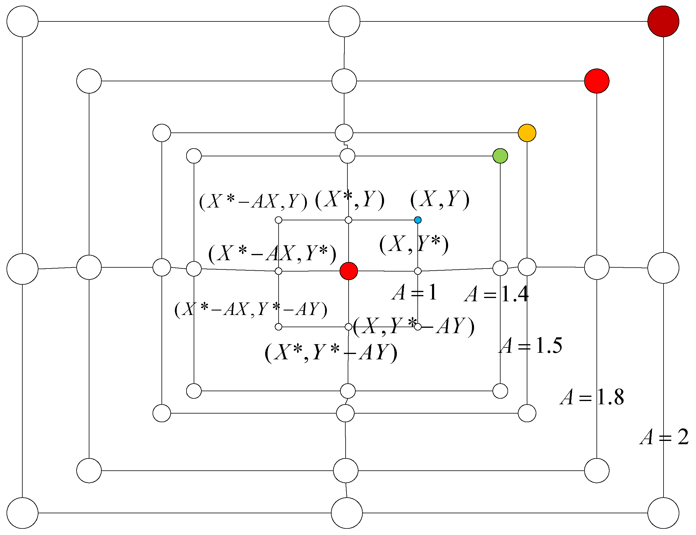
where, ${\overrightarrow{X}}_{rand}$ is a random location vector selected from the current population. Figure 1 shows a possible location of a solution when $\overrightarrow{A}>1$. When $\left|\overrightarrow{A}\right|>1$, the search agent selects a random agent, and when $\left|\overrightarrow{A}\right|<1$, the search agent is selected as the current best agent to replace the location of the search agent.

2.3. Encircling Prey

At the initial stage, the optimal location in the search space is unknown when the prey is surrounded. In this algorithm, the best candidate is regarded as the target prey or the best target. After that, the best search agent will be defined, and other agents will try to update their location toward the best agent. The mathematical model of this behavior can be described as follows:

$$\overrightarrow{D}=\left|\overrightarrow{C}\cdot {\overrightarrow{X}}^{*}(t)-\overrightarrow{X}(t)\right|$$

(3)

$$\overrightarrow{X}(t+1)={\overrightarrow{X}}^{*}(t)-\overrightarrow{A}\cdot \overrightarrow{D}$$

(4)

where t is the current iteration number, $\overrightarrow{A}$ and $\overrightarrow{C}$ are the coefficient vector, $X^{*}$ is the known optimal location vector, $\overrightarrow{X}$ is the location vector of other search agents. It is proposed that, in each iteration, if a better solution occurs, the $X^{*}$ will be replaced with a better one.

The calculated expressions of $\overrightarrow{A}$ and $\overrightarrow{C}$ are described follows:

$$\overrightarrow{A}=2\mathrm{a}\cdot \overrightarrow{\mathrm{r}}-\mathrm{a}$$

(5)

$$\overrightarrow{C}=2•\overrightarrow{\mathrm{r}}$$

(6)

The $\mathrm{a}$ is linearly reduced in the interval (0, 2) in the iterative process (including the whole exploration and development phase), and the vector $\overrightarrow{\mathrm{r}}$ is a random vector in interval [0,1]. Figure 2 illustrates the theoretical basis of Equation (4) in two dimensional plane. The search agent (X, Y) can update its location based on the location of the current best agent ($X^{*}$, $Y^{*}$). It can be seen from this point that if the choice of ($X^{*}$, $Y^{*}$) is not good, it will be easy to make the algorithm fall into the local optimum. It can be seen from Figure 2 that anywhere near the best agent can be achieved by changing the value of the $\overrightarrow{A}$ and $\overrightarrow{C}$.

2.4. Bubble-Net Attacking Method (Exploitation Phase)

The third stage is the bubble-net attacking method. In order to realize the model in this stage, two ideas are introduced.

1.

Shrinking encircling mechanism

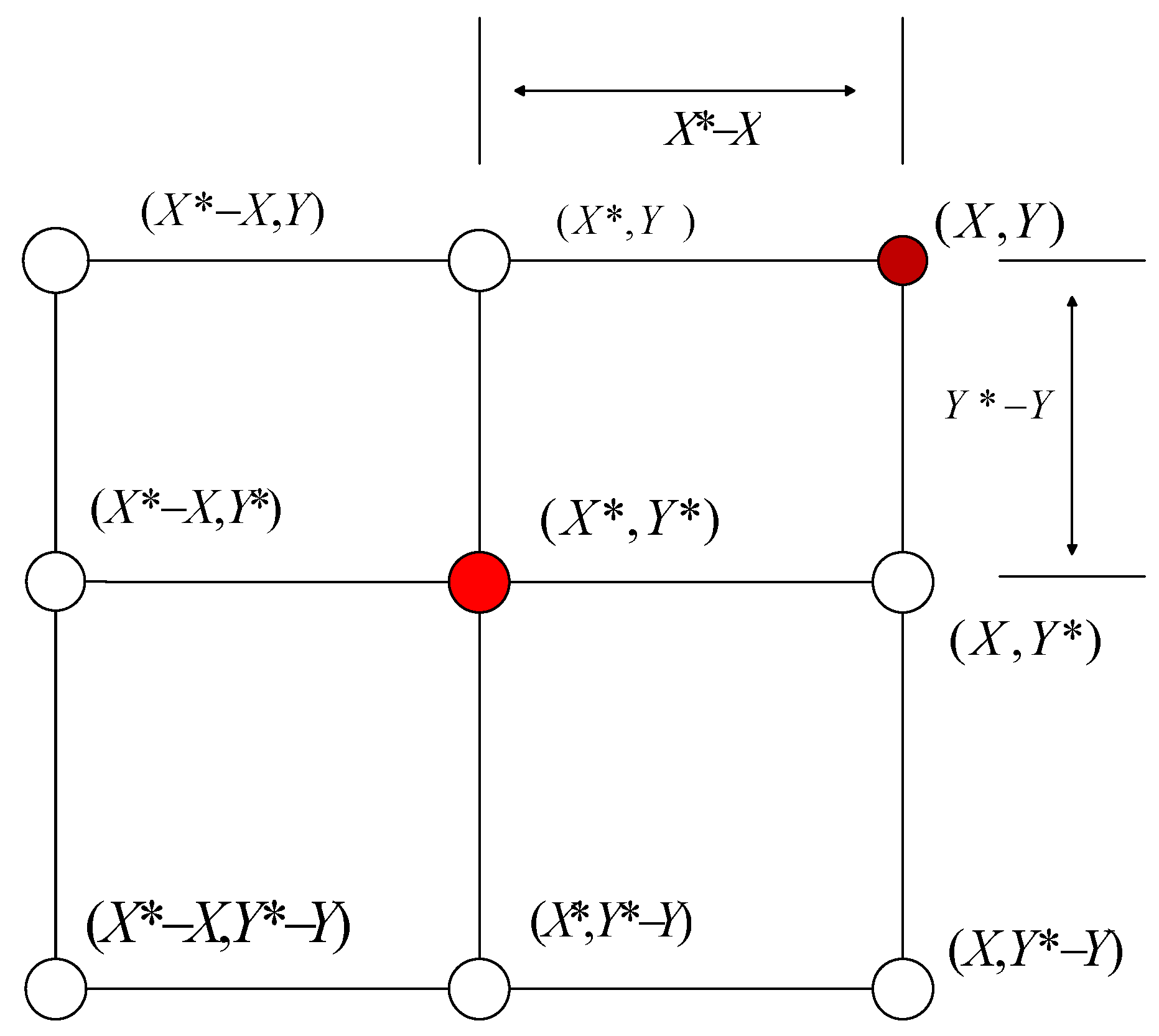
By reducing the value of $\mathrm{a}$ in Equation (5), the value of $\overrightarrow{A}$ is limited in [−a, a]. When random values for $\overrightarrow{A}$ are in the interval [−1,1], the new search agent can be defined any location between the initial position and the current search agent’s best position. The theoretical illustration of the shrinking encircling mechanism is shown in Figure 3. It can be seen that any position between (X, Y) and ($X^{*}$, $Y^{*}$) in the two dimensional plane can be reached by adjusting the value of A between [0,1].

2.

Spiral updating position method

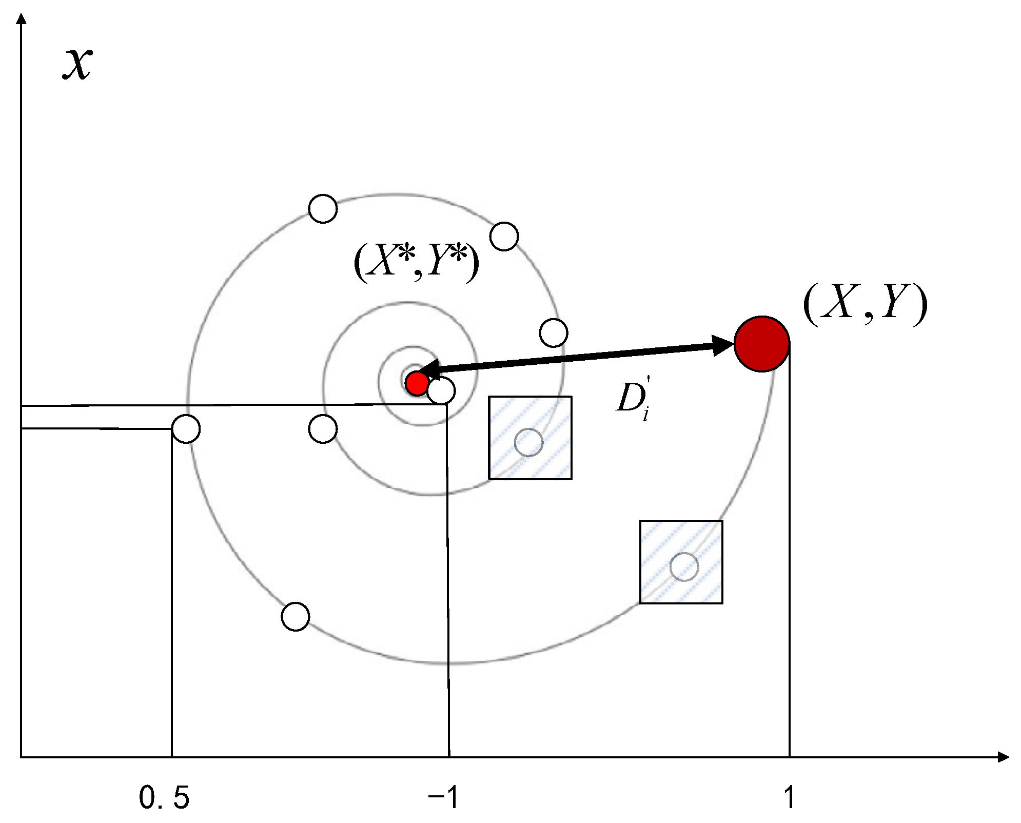
The sketch map of spiral renewal position method is shown in Figure 4, which is the path of the search agent proposed by the original WOA. It calculates the distance between whale (X, Y) and ($X^{*}$, $Y^{*}$) prey. The equation imitating the humpback whales spiral moving mode is described as follows.

$$\overrightarrow{X}(\mathrm{t}+1)=\overrightarrow{D^{\prime }}\cdot e^{bl}\cdot \cos (2\pi l)+{\overrightarrow{X}}^{*}(t)$$

(7)

where, $\overrightarrow{D^{\prime }}=\left|{\overrightarrow{X}}^{*}(t)-\overrightarrow{X}(t)\right|$ represents the distance between the $i$th whale and the prey, b is used to define the constant to limit the logarithmic spiral and $l$ is a random number between the interval [−1,1].

To be mentioned, the humpback whales swim around the prey in a gradual contraction of the circle and a spiral shape. In order to facilitate the establishment of the model, it is stipulated that each of the fifty percent of the whales may choose to surround the contraction path or spiral model to update their locations. The mathematical model is described as follows.

$$\overrightarrow{X}(t+1)=\{\begin{array}{ll}{\overrightarrow{X}}^{*}(t)-\overrightarrow{A}\cdot \overrightarrow{D}& p<0.5\\ \overrightarrow{D^{\prime }}\cdot e^{bl}\cdot \cos (2\pi l)+{\overrightarrow{X}}^{*}(t)& p\ge 0.5\end{array}$$

(8)

where, $p$ is a random number between [0,1].

2.5. Idea of Improving Whale Optimization Algorithm

Through carrying out the research on the original WOA idea, two improvement ideas are put forward.

(1) It can be seen from the searching path of the whales in Figure 4 and Equation (7), the logarithmic spiral curve adopted as the searching path, but the pitch is not equal seen from the logarithmic helix curve. In other words, when the searching agent carries out the searching process according to the path, it can be seen from the two shaded sections in Figure 2 that any location around the best agent can be changed by changing the values of $\overrightarrow{A}$ and $\overrightarrow{C}$. However, if the pitch of the spiral curve is larger than that of the search agent, it will lead to some locations can not be searched so as to reduce the ergodicity of the algorithm.

(2) In order to make the algorithm search thoroughly near the location of the search agents, after each iteration of the WOA, a set of more advantageous searched positions $X^{*}(t)$ are obtained. Then $X^{*}(t)$ will be no go directly into the next iteration, the disturbance is carried on it so as to searching the nearby scope of $X^{*}(t)$. The next iteration will generate a new best searching agent.

3. Complex Path-Perceptual Disturbance WOA

3.1. Selection of Mathematical Model of Searching Path

According to the logarithmic spiral model proposed by the original WOA, seven kinds of spirals are puts forward as the mathematical models of searching paths [40].

3.1.1. Logarithmic Spiral Curve (Lo)

Logarithmic spiral curve is also called equilateral spiral curve. The mathematical model of Logarithmic spiral searching path is described in Equation (9) and the two-dimensional image is show in Figure 5.

$$\{\begin{array}{c}x=a\cdot e^l\cos (2\pi l)\\ y=a\cdot e^l\sin (2\pi l)\end{array}$$

(9)

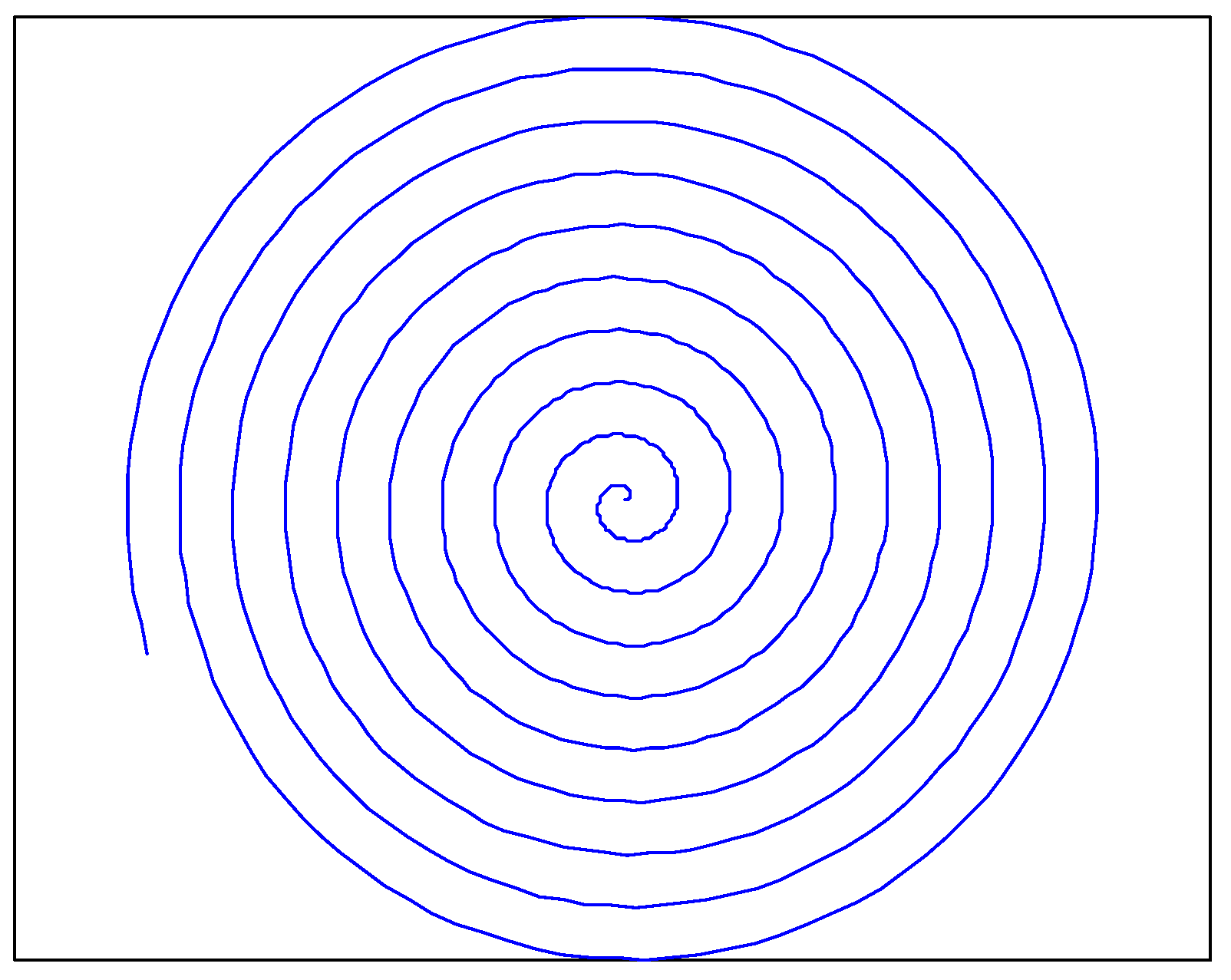
3.1.2. Archimedes Spiral Curve (Ar)

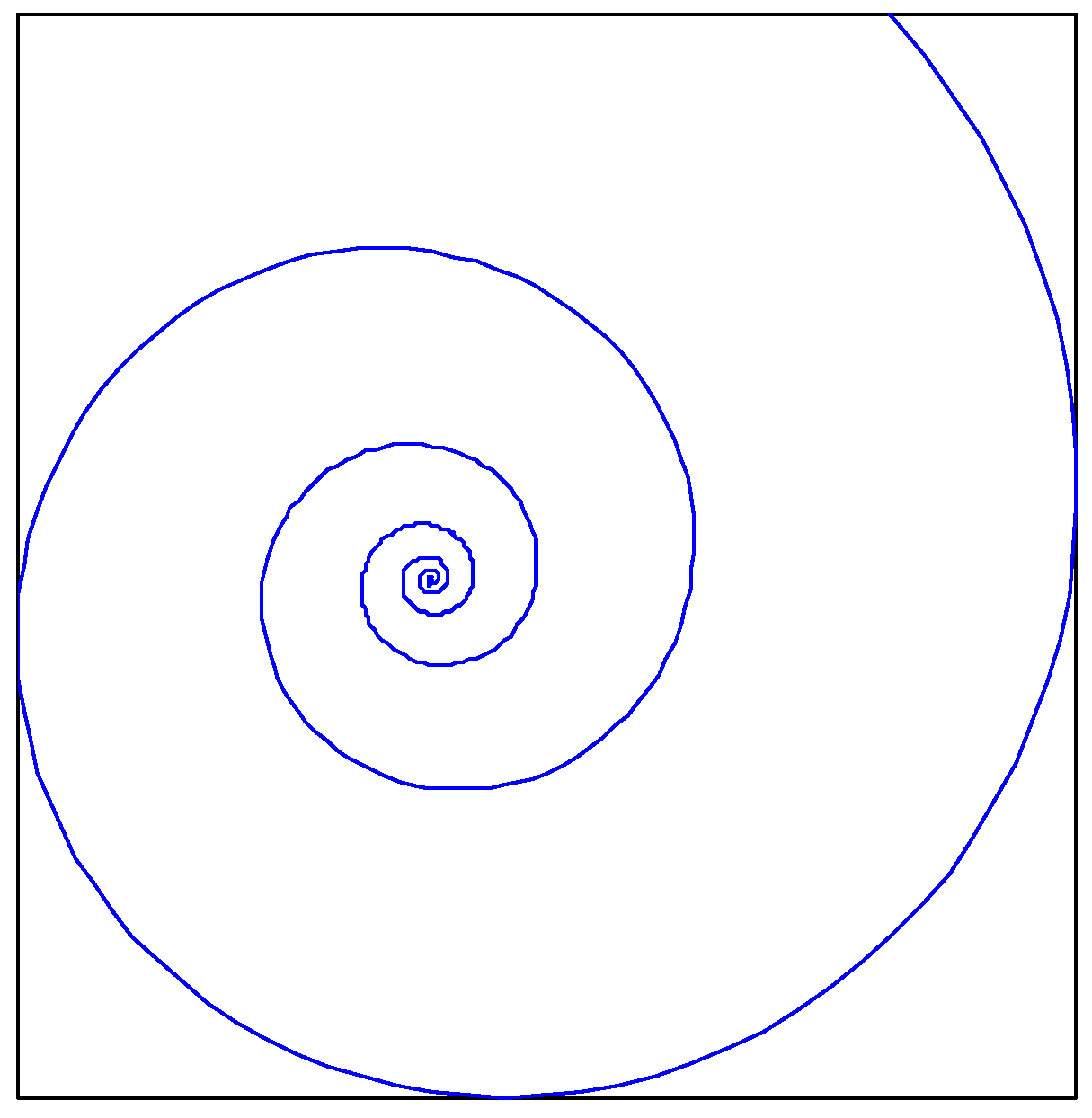
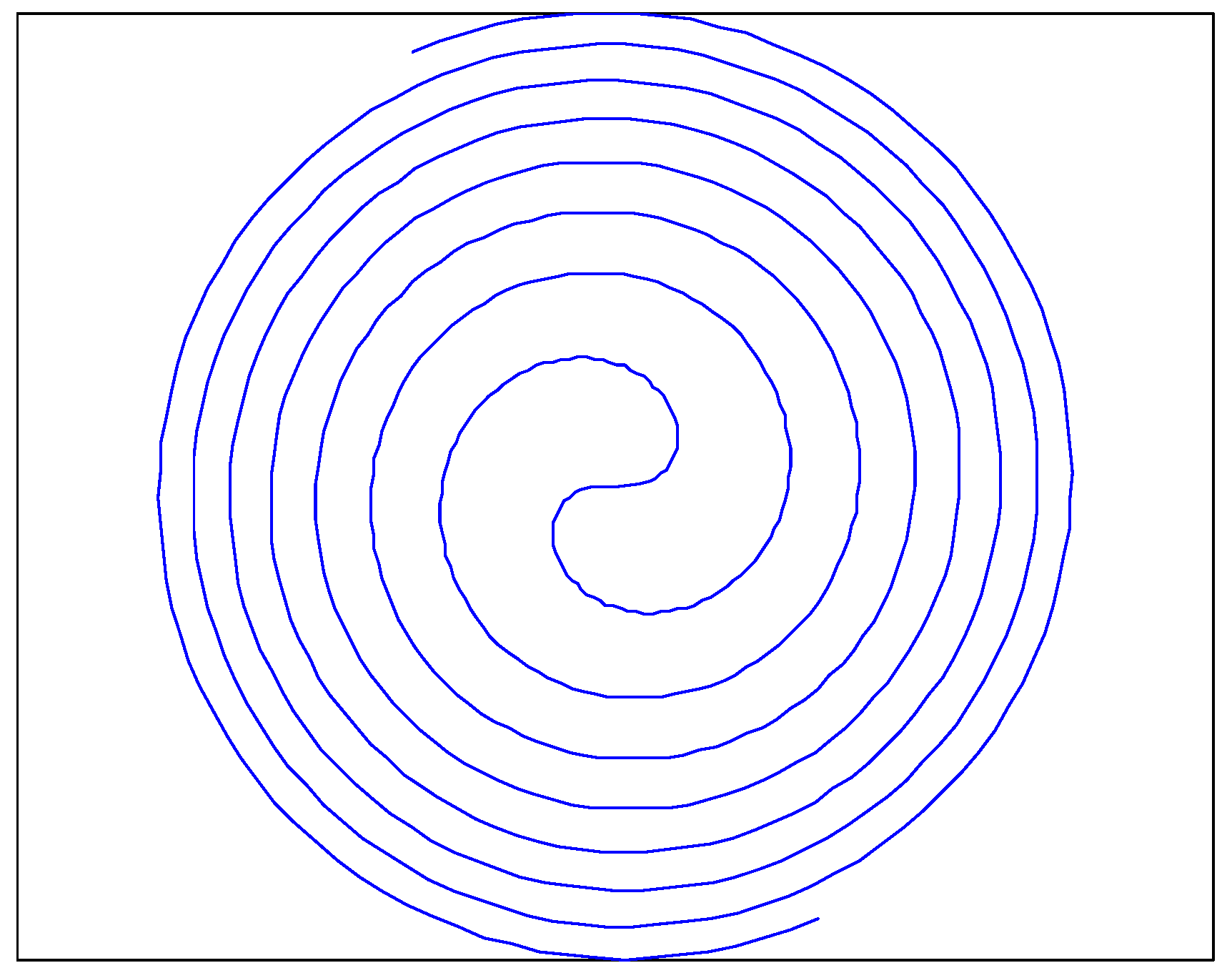
The Archimedes spiral curve is a trail generated by a point evenly moving away from a fixed point, while moving at a fixed angular velocity around the fixed point. The equal pitch Archimedes spiral means that the pitch of the spiral curve is a invariant constant shown in Figure 6. The mathematical model of Archimedes spiral searching path is described in Equation (10) and the two-dimensional image is show in Figure 6.

$$\{\begin{array}{c}x=(a+b\cdot l)\cos (2\pi l)\\ y=(a+b\cdot l)\sin (2\pi l)\end{array}$$

(10)

As we put forward, the pitch of the spiral curve gradually changes to affect the convergence performance of the algorithm. Therefore, we first select the Archimedean spiral curve with a constant pitch. Since its pitch is equidistant, we use an algorithm to adjust the parameters of the function so that the algorithm achieves optimal performance.

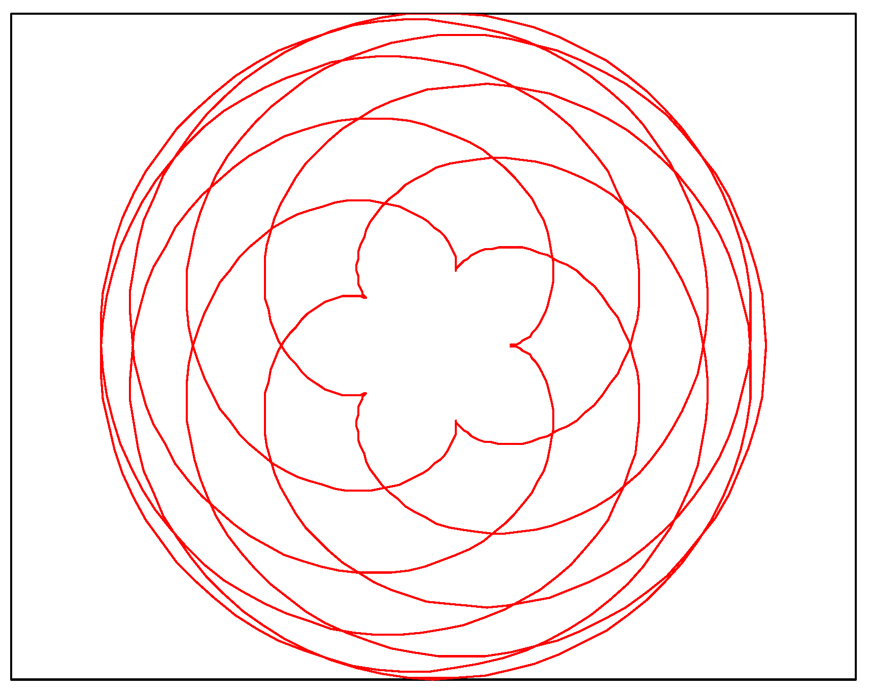
3.1.3. Rose Spiral Curve (Ro)

Assuming a fixed length segment AB = 2a, the two endpoints of AB slide on two mutually perpendicular straight lines. Then a vertical line OM is made from the intersection O of two straight lines to the line AB. The trajectory of foot M is called the Rose spiral curve. The mathematical model of Rose spiral with four leaves searching path is described in Equation (11) and the two-dimensional image is show in Figure 7.

$$\{\begin{array}{c}x=a\cdot \cos (n\pi l)\sin (l)\\ y=a\cdot \sin (n\pi l)\cos (l)\end{array}$$

(11)

Because the path of the function is relatively simple, taking into account the existence of the disturbance, by adjusting the parameters of the function, the spacing between the search paths is as small as possible, and the optimal value may be obtained faster with as few iterations as possible. So we chose this spiral curve.

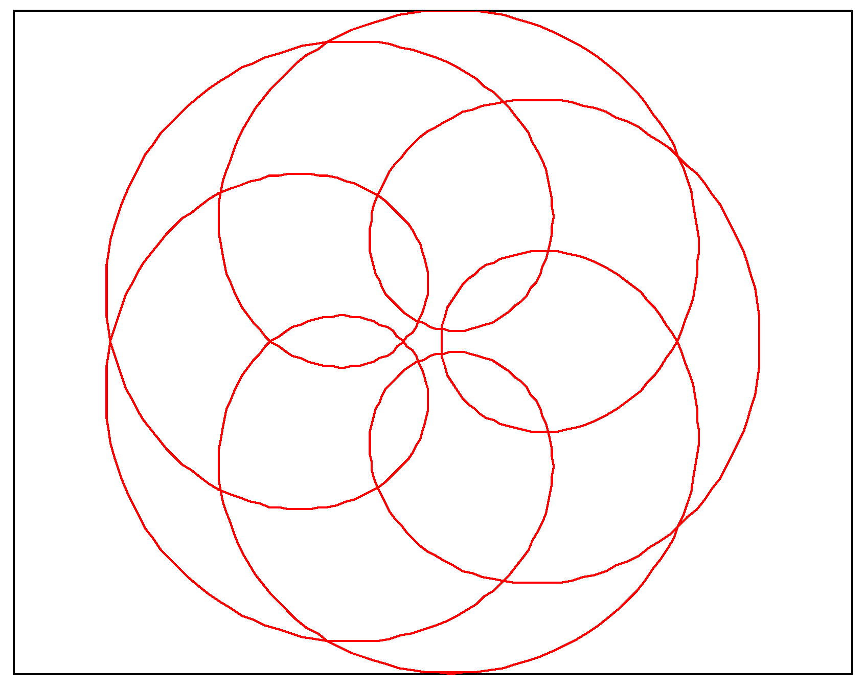
3.1.4. Epitrochoid-I (Ep-I)

A movable circle is carried out the roll around the externally-tangent of the fixed circle internally, where the radius of the fixed circle is $a$ and the radius of the movable circle is $b$. In the process of the movable circle rolling, the trajectory is formed by a fixed point $P$ on the movable circle, which is called the Epicycloid-I. The mathematical model of Epitrochoid-I searching path is described in Equation (12) and the two-dimensional image is show in Figure 8.

$$\{\begin{array}{c}x=(a+b)\cdot \cos (n\pi l)-c\cos (\frac{a}{b+1}n\pi l)\\ y=(a+b)\cdot \sin (n\pi l)+c\sin (\frac{a}{b+1}n\pi l)\end{array}$$

(12)

3.1.5. Hypotrochoid (Hy)

A fixed large circle internally tangent a movable small circle. In the process of small circle rolling, the trajectory is formed by a fixed point $P$ on the small circle, which is called the Hypotrochoid. The curve will change with the radius of the two circles. The mathematical model of Hypotrochoid searching path is described in Equation (13) and the two-dimensional image is show in Figure 9.

$$\{\begin{array}{c}x=(a+b)\cdot \cos (n\pi l)-b\cos (\frac{a}{b+1}n\pi l)\\ y=(a+b)\cdot \sin (n\pi l)-b\sin (\frac{a}{b+1}n\pi l)\end{array}$$

(13)

3.1.6. Epitrochoid-II (Ep-II)

The formation principle of the Epicycloid-II and the Epicycloid-I is the same. Just the difference of the radius of the big circle and the small circle produces the different trend. The mathematical model of Epitrochoid-II searching path is described in Equation (14) and the two-dimensional image is show in Figure 10.

$$\{\begin{array}{c}x=(a-b)\cdot \cos (n\pi l)+c\cos (\frac{a}{b-1}n\pi l)\\ y=(a-b)\cdot \sin (n\pi l)-c\sin (\frac{a}{b-1}n\pi l)\end{array}$$

(14)

The selection idea of the three spiral curves of EP-I, EP-II, and Hy is that when multiple agents are searching at the current optimal position, the agent performs a full search around the current optimal position according to its search path.

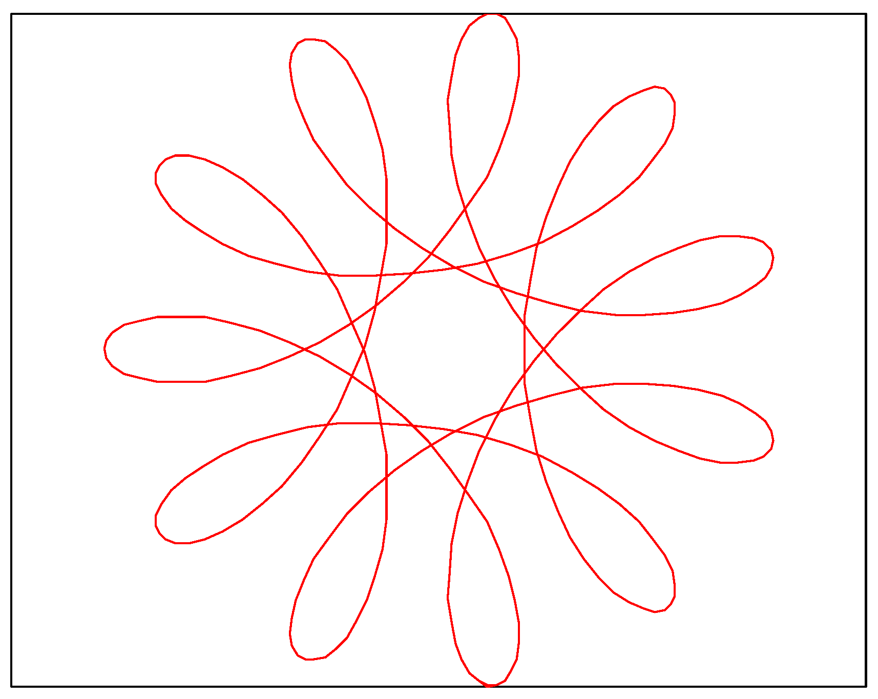
3.1.7. Fermat Spiral Curve (Fe)

The Fermat spiral curve is a kind of equiangular spiral curve. It is obtained by tire up the starting points of the two logarithmic spiral curves, whose rotation direction is opposite. The mathematical model of Fermat spiral searching path is described in Equation (15) and the two-dimensional image is show in Figure 11.

$$\{\begin{array}{c}x=\sqrt{l}\cos (\frac{a}{b-1}n\pi l)\\ y=-\sqrt{l}\sin (\frac{a}{b-1}n\pi l)\end{array}$$

(15)

3.1.8. Lituus Spiral Curve (Li)

The Lituus spiral curve is parameterized and interacted by three helical curves. The mathematical model of Lituus spiral searching path is described in Equation (16) and the two-dimensional image is show in Figure 12.

$$\{\begin{array}{c}x=\sqrt{\frac{a+b}{l}}\cos (\frac{a}{b-1}n\pi l)\\ y=-\sqrt{\frac{a+b}{l}}\sin (\frac{a}{b-1}n\pi l)\end{array}$$

(16)

Li and Fe, we complete the search path corresponding to such functions by defining the positive and negative of two search agents. Search for larger ranges in less time by combining two agents searching in symmetrical positions.

3.2. Introduction of Disturbance Factor

In order to make the WOA search thoroughly near the location of the search agent, after each iteration, a set of more advantageous search positions $X^{*}(t)$ are obtained. But it will not go directly to the next iteration. A disturbance factor is carried out to search the nearby scope of $X^{*}(t)$. The next iteration will generate a new best search agent. In order to get rid of the randomness and blindness of the original perturbation method, when constructing the perturbation factor, the range of disturbances are limited to ensure the accuracy of local search. At the same time, in order to make the search agents swim to the targets in the disturbance range as far as possible. Then the perceptual coefficient is introduced. In this way, the search agents are constantly changing the positions within the disturbance range and the optimal value are replaced with the current optimal. The introduced disturbance factor is described as follows.

$$\epsilon =\frac{x_d-x}{\Vert x_d-x\Vert }\cdot Step\cdot Rand()$$

(17)

After the disturbance, the position of the search agent is updated by the following equation.

$$x=x+u\cdot Rand()\oplus \epsilon$$

(18)

where, $u$ is the coefficient that defines the perturbation distance, $Rand()$ is a random number between (−1, 1), $Step$ is the step size of the search agent moving at the time of disturbance, $x_d$ is the position at time $d$, $x$ is the current best position, $\oplus$ represents the point-to-point multiplication.

In the Equation (18), $(x_d-x)/\Vert x_d-x\Vert$ is selected for the nature of fitness function, when the fitness function solves the maximum value problem, select $(x_d-x)/\Vert x_d-x\Vert$; if the minimum value is solved, then $(x_d-x)/\Vert x_d-x\Vert$ is selected. When the perturbation result is unchanged, the disturbed structure is allowed to enter the next main loop.

3.3. Improved WOA with Perceptual Disturbances and Complex Paths

The algorithm should search out a better position as fast as possible in the initial period of the disturbance. In the later stages of the perturbation, the search agent can perform a more thorough search near the target to improve the search accuracy. For the above given formula, the moving step size of the search agents is redefined as:

$$\begin{array}{l}Step=Ste{p}_{\min }+(Ste{p}_{\max }-Ste{p}_{\min })\times \frac{N-n}{N}\\ s.t.\begin{array}{cc}& if\end{array}Step>Ste{p}_{\max }\\ \begin{array}{ccc}& then& Step=Ste{p}_{\max }\end{array}\end{array}$$

(19)

where $Ste{p}_{\min }$ is the minimum value of the moving step, $Ste{p}_{\max }$ is the maximum value of the moving step, $N$ is the maximum number of iterations and $n$ is the current number of iterations.

It can be seen from the above equations, the value of $Step$ is the maximum value from the beginning of the iteration and the minimum at the end of the iteration. The algorithm procedure of the complex path-perceptual disturbance WOA (CP-PDWOA) is described as follows.

Step 1: Initialization. Randomly generate $N$ search agents and initialize their locations.

Step 2: Realization of searching path. In this paper, the moving path of the search agents is improved, but the shrinking idea of the searching path is constant. Randomly generate a number $p\in (0,1)$. When $p<0.5$, the shrinking encircling mechanism is executed so as to narrow the search radius. When $p>0.5$, the method of the spiral updating position is executed. The above two steps are not followed by order and are random implemented.

Step 3: Update locations. The value of $\left|\overrightarrow{A}\right|$ in Equation (5) is the criterion for the search agent to update the next location. When $\left|\overrightarrow{A}\right|\ge 1$, the search agent randomly selects an agent as a reference for the next move, which is to ensure the ergodicity of the algorithm. When $\left|\overrightarrow{A}\right|\le 1$, the search agent chooses the current optimal agent as the reference for the next move, which is to ensure the convergence of the algorithm.

Step 4: Perceived perturbation. The best search agent at each iteration is disturbed. Then the position of the search agent is tested after the perturbation, and the test result is compared with the search agent obtained from the last disturbance to select the position of the better search agent. After a number of disturbances, a good set of search agents is obtained, and the best position $X_{best}$ is selected.

Step 5: Determine whether to terminate the iteration. If the fitness value $f(X_{best})$ reaches the termination condition, $X_{best}$ is the optimal solution. If it does not reached, the solution group obtained by Step 4 returned to Step 2 for the next iteration.

It must be explained that Step 2 and Step 3 are executed at the same time when the algorithm is ran. In this paper, it is decomposed into two steps in order to facilitate the expression.

4. Simulation and Results Analysis

4.1. Selection of Testing Functions

In order to test the performance of the improved WOA, 23 benchmark functions are selected in this paper [41,42]. The expressions of the functions are shown in

Table 1. Testing functions.

Function	Function Expression	Range	Fmin
F1	$f_1(x)={\displaystyle \sum _{i=1}^d{x}_i^2}$	[−100,100]	0
F2	$f_2(x)={\displaystyle \sum _{i=1}^d\left|x_i\right|}+{\displaystyle {\prod }_{i=1}^n\left|x_i\right|}$	[−10,10]	0
F3	$f_3(x)={{\displaystyle \sum _{i=1}^d\left({\displaystyle {\sum }_{j-1}^i{x}_j}\right)}}^2$	[−100,100]	0
F4	$f_4\left(x\right)={\max }_i\left\{\left|x_i\right|,1\le i\le n\right\}$	[−100,100]	0
F5	$f_5(x)={\displaystyle \sum _{i=1}^{d-1}(100(x_{i+1}-x_i{}^2)+{(x_i-1)}^2)}$	[−30,30]	0
F6	$f_6\left(x\right)={\displaystyle {\sum }_{i=1}^d{\left([x_i+0.5]\right)}^2}$	[−100,100]	0
F7	$f_7\left(x\right)={\displaystyle {\sum }_{i=1}^{d}i{x}_i^4+random[0,1)}$	[−1.28,1.28]	0
F8	$f_8\left(x\right)={\displaystyle {\sum }_{i=1}^n-x_i}\sin \left(\sqrt{x_i}\right)$	[−500,500]	−418.9 $\times$ 5
F9	$f_9(x)={\displaystyle \sum _{i=1}^d(x_i{}^2-10cos(2\pi x_i)+10)}$	[−5.12,5.12]	0
F10	$\begin{array}{l}{f}_{10}\left(x\right)=-20\exp \left(-0.2\sqrt{\frac{1}{n}{\displaystyle {\sum }_{i=1}^n{x}_i^2}}\right)-\exp \left(\frac{1}{n}{\displaystyle {\sum }_{i=1}^n\cos \left(2\pi x_i\right)}\right)\\ +20+e\end{array}$	[−32,32]	0
F11	$f_{11}(x)=\frac{1}{4000}\left({\displaystyle \sum _{i=1}^n(x^{2}i)}\right)-\left({\displaystyle \prod _{i=1}^n\cos (\frac{xi}{\sqrt{i}})}\right)+1$	[−600,600]	0
F12	$\begin{array}{l}{f}_{12}\left(x\right)=\frac{\pi }{n}\left\{10\sin \left(\pi y_1\right)+{\displaystyle {\sum }_{i=1}^{n-1}{\left(y_i-1\right)}^2\left[1+10{\sin }^2(\pi y_{i+1}\right]+{(y_n+1)}^2}\right\}\\ +{\displaystyle {\sum }_{i=1}^{n}u(x_i},10,100,4)\end{array}$$y_i=1+\frac{x_i+1}{4};u(x_i,a,k,m)=\{\begin{array}{c}k{(x_i-a)}^m\\ 0\\ k{(-x_i-a)}^m\end{array}\begin{array}{c}{x}_i>a\\ -a<x_i<a\\ x_i<-a\end{array}$	[−50,50]	0
F13	$\begin{array}{l}{f}_{13}\left(x\right)=0.1\{{\sin }^2\left(3\pi x_1\right)+{\displaystyle {\sum }_{i=1}^n{\left(x_i-1\right)}^2\left[1+{\sin }^2(3\pi x_{i+1})\right]}\\ +{(x_n-1)}^2\left[1+{\sin }^2(3\pi x_{i+1})\right]\}+{\displaystyle {\sum }_{i=1}^{n}u(x_i},5,100,4)\end{array}$	[−50,50]	0
F14	$f_{14}={(\frac{1}{500}+{\displaystyle {\sum }_{j=1}^{25}\frac{1}{j+{\displaystyle {\sum }_{i=1}^2{(x_i-a_{ij})}^6}}})}^{-1}$	[−65,65]	1
F15	$f_{15}={\displaystyle {\sum }_{i=1}^{11}[a_i-\frac{x_1(b_i^2+b_1{x}_2)}{b_i^2+b_1{b}_3+b_4}}{]}^2$	[−5,5]	0.0003
F16	$f_{16}=4x_1^2-2.1x_1^4+\frac{1}{3}x{}_1{}^6+x_1{x}_2-4x_2^2+4x_2^4$	[−5,5]	−1.0316
F17	$f_{17}={(x_2-\frac{5.1}{4{\pi }^2}{x}_1^2+\frac{5}{\pi }{x}_1-6)}^2+10(1-\frac{1}{8\pi })\cos x_1+10$	[−5,5]	0.398
F18	$\begin{array}{l}{f}_{18}=[1+{(x_1+x_2+1)}^2(19-14x_1+3x_1^2+6x_1{x}_2+3x_2^2)]\\ \begin{array}{cc}& \times [30+{(2x_1-3x_2)}^2]\end{array}\times (18-32x_1+12x_1^2+48x_2-36x_1{x}_2+27x_2^2))\end{array}$	[−2,2]	3
F19	$f_{19}=-{\displaystyle {\sum }_{i=1}^4{c}_i}\exp (-{{\displaystyle {\sum }_{j=1}^3{a}_{ij}(x_{ij}-p_{ij})}}^2)$	[1,3]	−3.80
F20	$f_{20}=-{\displaystyle {\sum }_{i=1}^4{c}_i}\exp (-{{\displaystyle {\sum }_{j=1}^6{a}_{ij}(x_{ij}-p_{ij})}}^2)$	[0,1]	−3.32
F21	$f_{21}=-{{\displaystyle {\sum }_{i=1}^5\left[(X-a_i){(X-a_i)}^T+c_i\right]}}^{-1}$	[0,10]	−10.1513
F22	$f_{22}=-{{\displaystyle {\sum }_{i=1}^7\left[(X-a_i){(X-a_i)}^T+c_i\right]}}^{-1}$	[0,10]	−10.4028
F23	$f_{23}=-{{\displaystyle {\sum }_{i=1}^{10}\left[(X-a_i){(X-a_i)}^T+c_i\right]}}^{-1}$	[0,10]	−10.5363

in details.

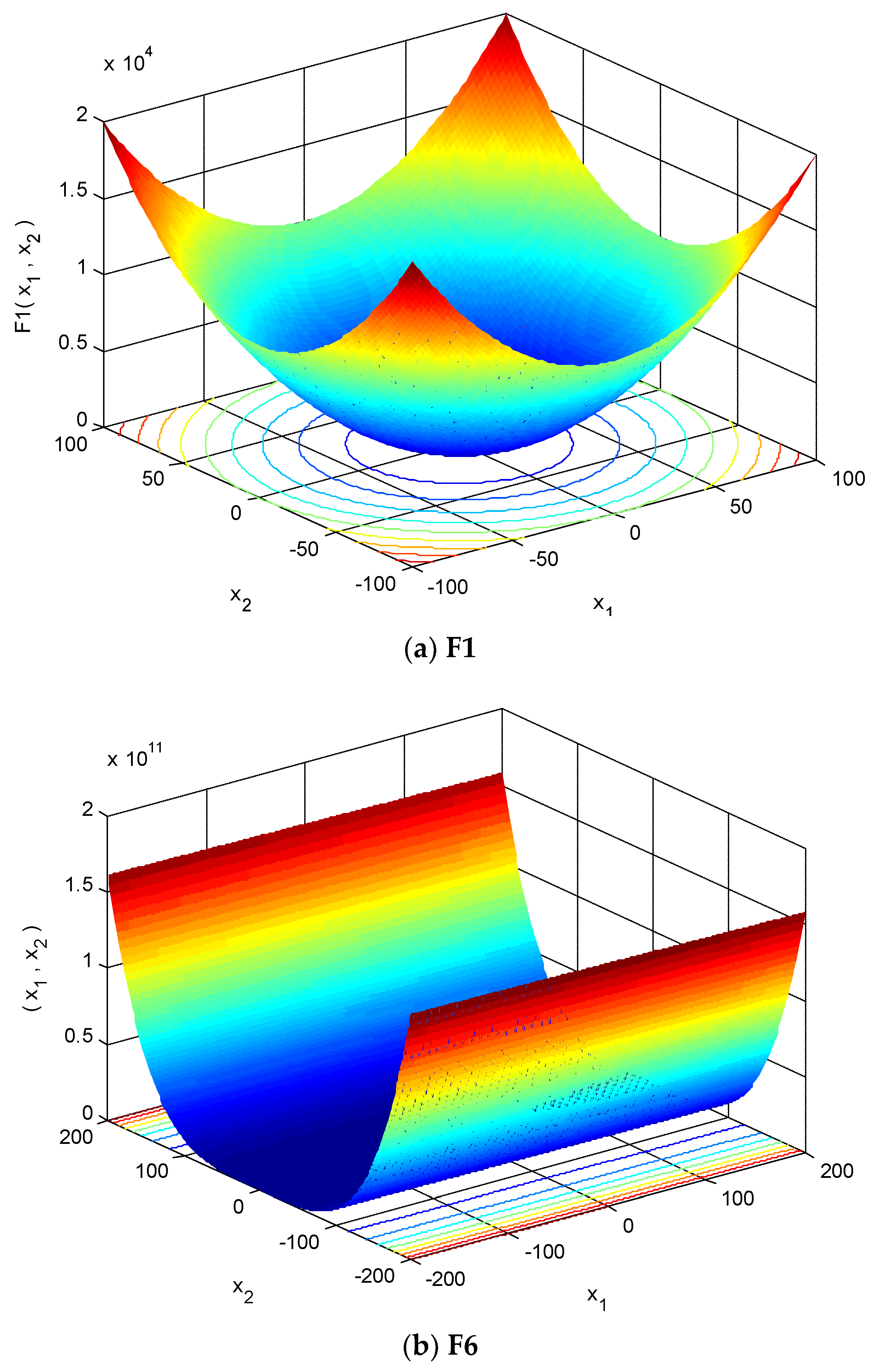
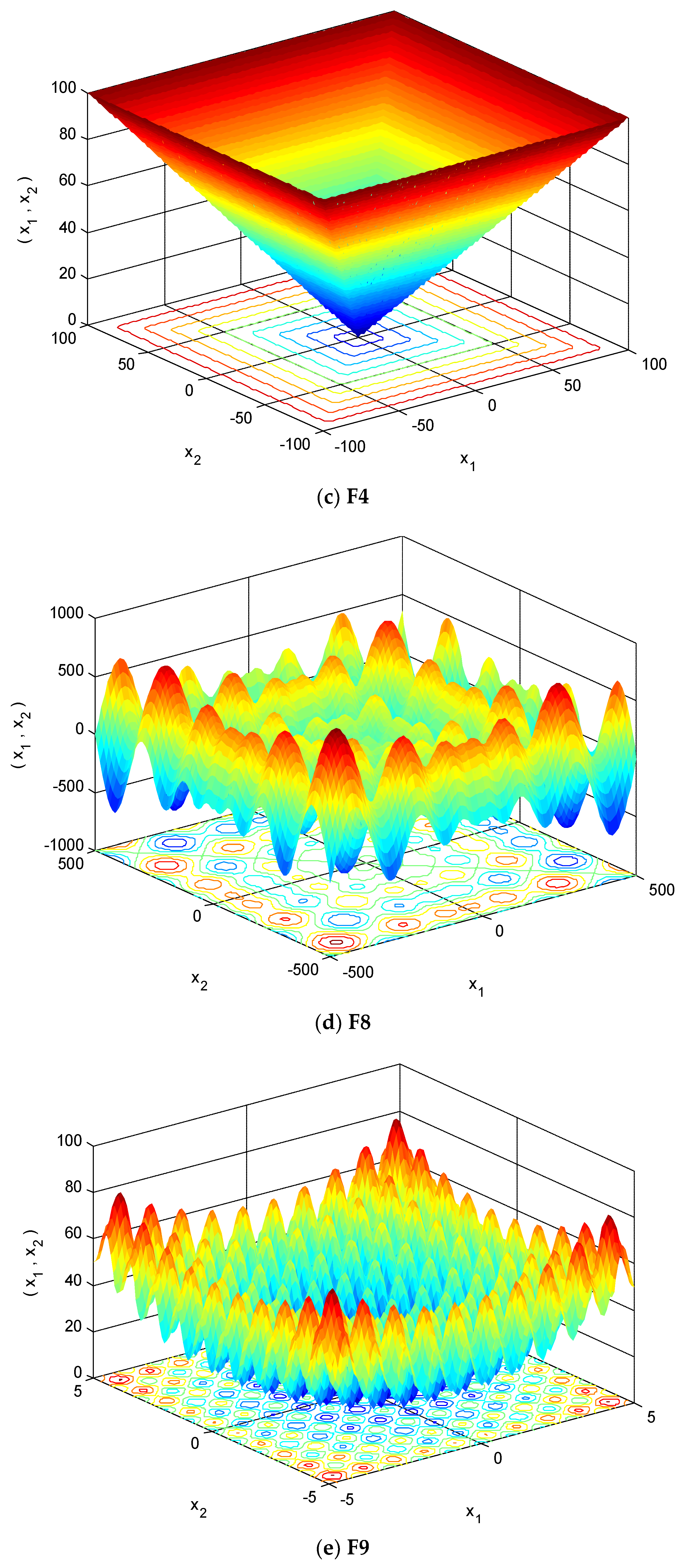
The three-dimensional images of a partial functions are shown in Figure 13a–i.

4.2. Simulation Results and Analysis

This paper tests the computational power of WOA by adopting 23 classical benchmark functions. Among them, the number of search agents is 30, the maximum number of iterations is 500. Each function runs 30 times and then takes the average to plot the convergence curve. Benchmark functions can be divided into four groups: unimodal, multimodal, fixed-dimension multimodal and composite functions. Functions F1–F7 are typical unimodal since they have only one global optimum. These functions allow to evaluate the exploitation capability of the investigated meta-heuristic algorithms. The functions F8–F23 are multimodal functions. Unlike unimodal functions, multimodal functions include many local optima whose number increases exponentially with the problem size (number of design variables). Therefore, this kind of test problems turns very useful if the purpose is to evaluate the exploration capability of an optimization algorithm.

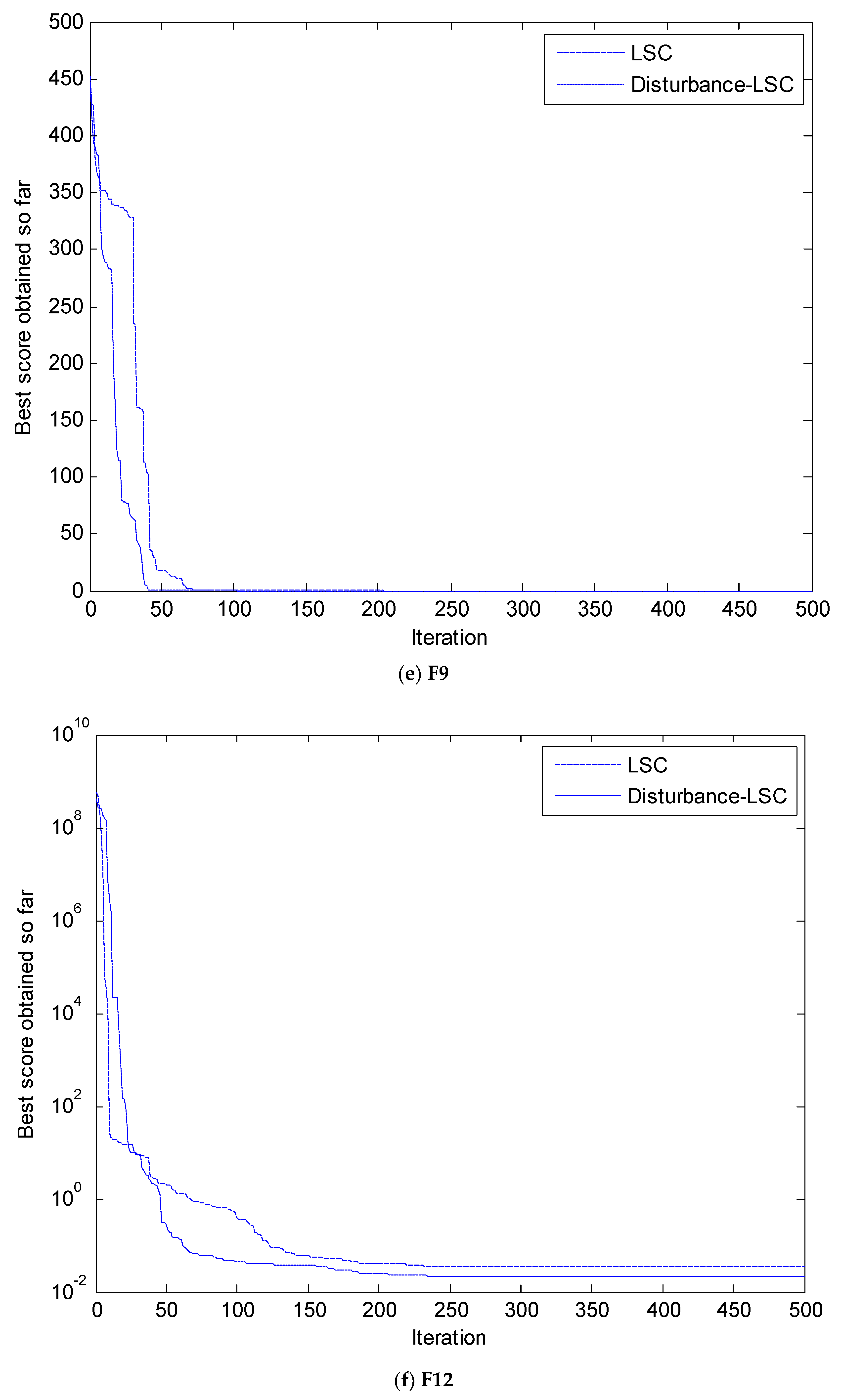
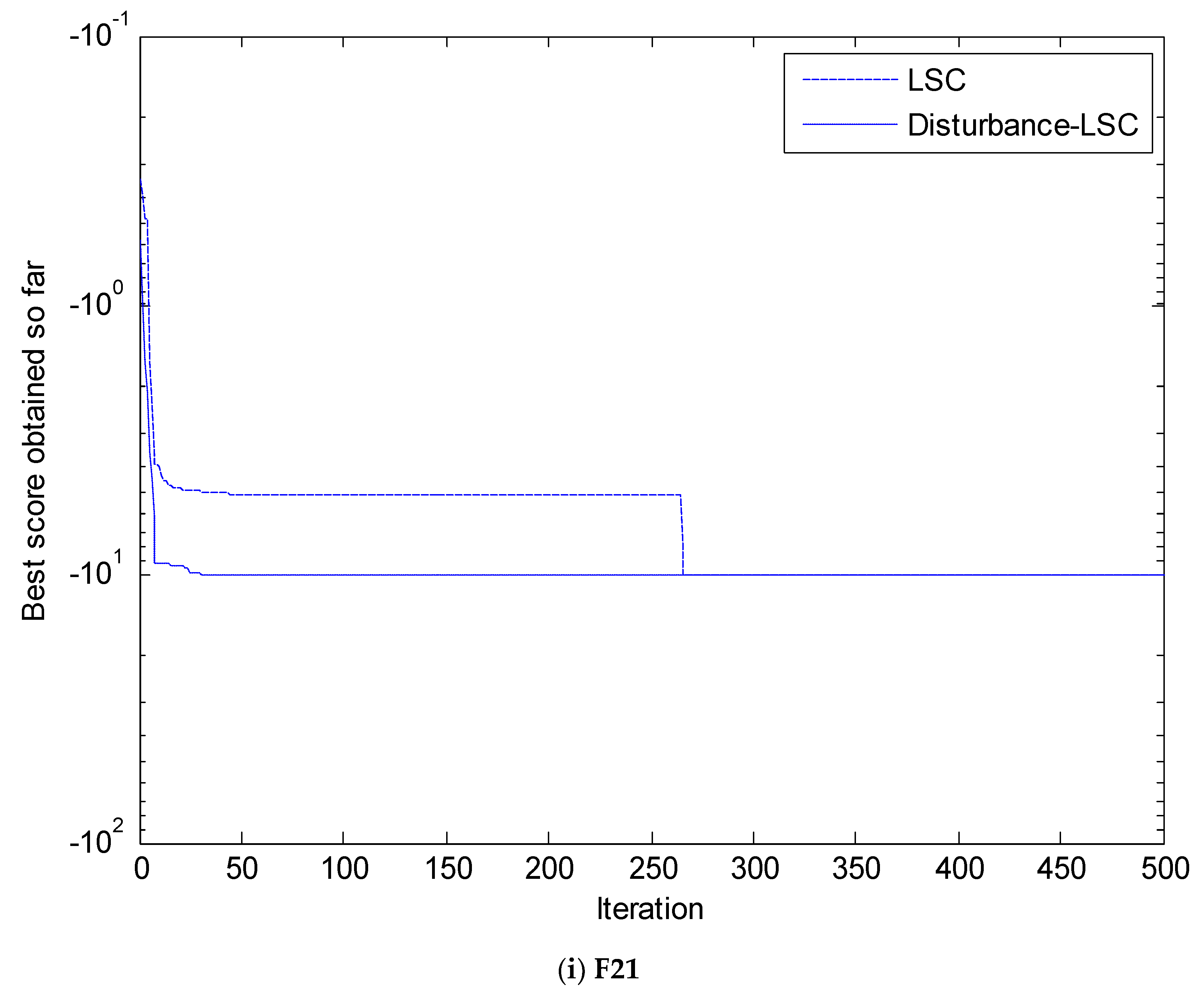
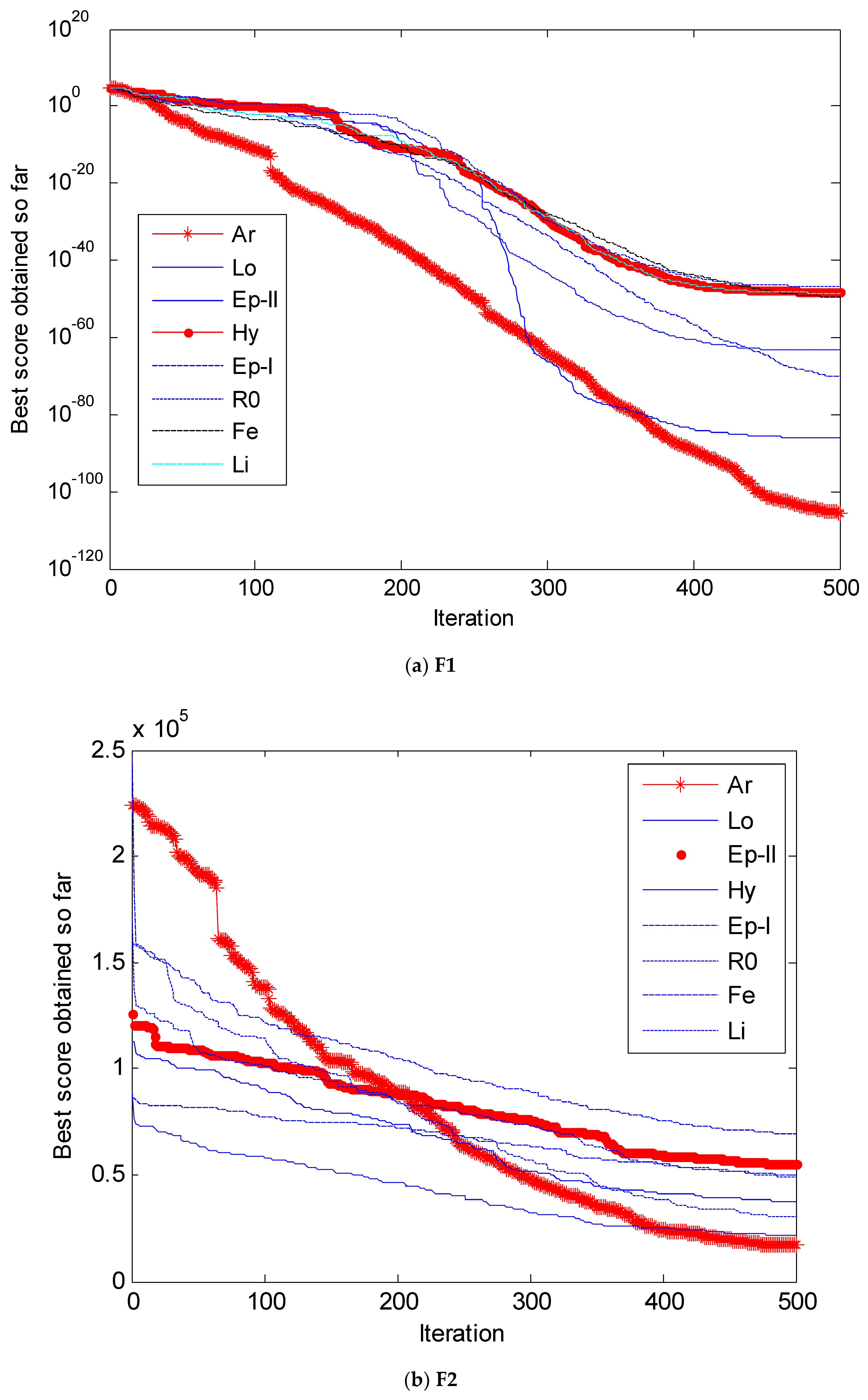
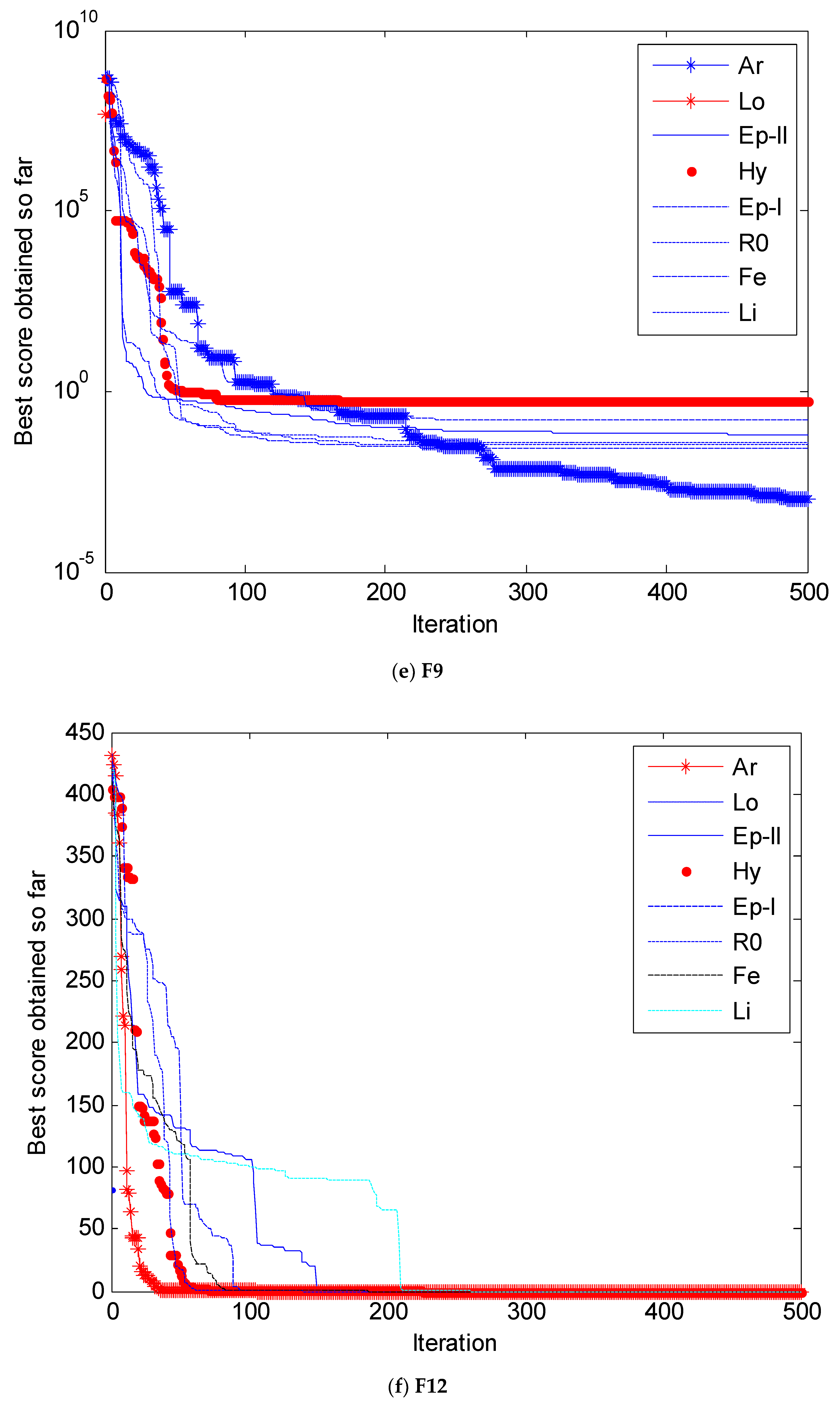
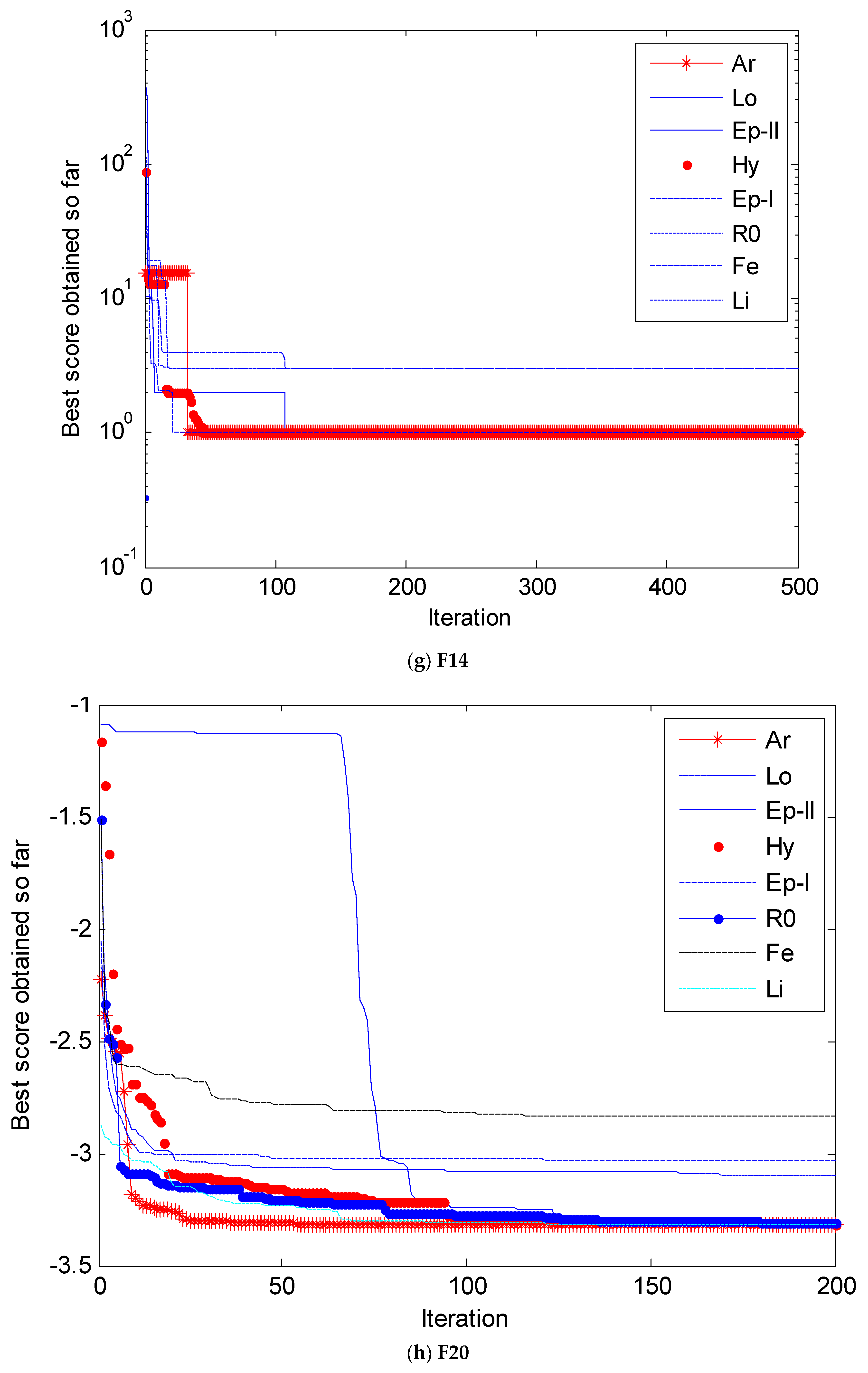
In this paper, we completed the simulation in matlab2010b environment, the computer configuration is Windows 7. The related MATLAB code of CP-PDWOA is available online at https://github.com/sunweizhen01/CP-PDWOA.git. Firstly, in order to verify the effectiveness of the perturbation mechanism, the convergence curves of the original WOA and the convergence curves after the introduction of the disturbance mechanism only with logarithmic spiral curve are compared. Then, the search path of the WOA with the disturbance mechanism is replaced by several spiral curves listed in Table 1 so as to find out the search path with the best optimization performance. The paper chooses several functions from above mentioned classes as a representative, and their convergence curves are shown in the following Figure 14 and Figure 15. The convergence performances of all the different methods are shown in

Table 2. Comparison of optimization results obtained for the unimodal, multimodal and fixed-dimension multimodal benchmark functions.

Function	L0		Ar		Ro		Hy		Pe-I		Pe-II		Fe		Li
	AVE	STD	AVE	STD	AVE	STD	AVE	STD	AVE	STD	AVE	STD	AVE	STD	AVE	STD
F1	1.41 × 10−30	4.91 × 10−30	3.64 × 10−106	4992.4116	2.065 × 10−47	6816.3959	1.001 × 10−48	8014.5287	1.031 × 10−86	6343.7262	7.242 × 10−71	5094.0843	3.096 × 10−60	5251.4799	3.638 × 10−49	7360.7530
F2	1.06 × 10−21	2.39 × 10−21	1.26 × 10−105	1012501	4.91 × 10−65	42530040813	8.33 × 10−43	19429812933	3.22 × 10−52	97498186729	3.22 × 10−52	5463750779	2.66 × 10−33	493771528062	4.66 × 10−36	14453630723
F3	21,533.06	15,903.34	17,308.09	61,432.76	49,342.12	22,646.55	37,706.46	22,712.248	55,440.039	19,449.57	50,199.04	10,850.31	69,415.32	25,663.15	30,810.03	36,337.14
F4	0.072581	0.39747	0.0240	10.750	8.1417	35.1489	7.8327	19.833	0.7614	5.7955	1.1439	15.942	1.0324	15.568	3.8082	24.589
F5	27.86558	0.763626	0.445	21966964	28.789	17463450	27.779	196730	10.637	197611	1.651	209162	8.598	258619	5.436	226382
F6	3.116266	0.532429	0.01752	8622.984	0.0001208	5866.599	0.010163	5806.449	0.01166	7645.330	0.00738	6855.553	0.01820	6264.7876	0.054570	4673.773
F7	0.001425	0.001149	0.000456	6.0642	0.00617	8.95037	0.001953	10.1904	0.00352	10.1742	0.00317	7.3495	0.00564	7.1875	0.000123	9.778
F8	−5080.76	695.7968	−12,569.062	882.164	−8103.505	784.832	−7574.253	385.518	−7747.811	421.263	−9937.307	625.755	−8163.108	395.22	−11,050.707	1125.405
F9	0	0	0	49.058	0	75.368	0	69.589	0	69.735	0	87.804	0	65.9588	0	60.5413
F10	7.4043	9.89757	8.88 × 10−16	2.9449	4.44 × 10−15	2.9965	4.44 × 10−15	3.5481	8.88 × 10−16	3.3239	8.88 × 10−16	3.0169	7.99 × 10−16	2.79940	1.39 × 10−13	3.05938
F11	0.00028	0.00158	9.9767 × 10−6	45.548	0	50.372	1.5259 × 10−10	62.525	7.414 × 10−10	54.537	1.1872 × 10−13	55.4545	0.00076571	66.1365	3.4649 × 10−5	50.2502
F12	0.33967	0.21486	0.00103	43593546	0.0335	48335777	0.5537	24074879	0.0631	46483837	0.1670	35041377	0.0273	39717531	0.0370	51384616
F13	1.88901	0.26608	0.0052	57915015	1.6642	73268462	0.1307	89315333	0.6859	96698854	0.2089	96675467	1.0066	68800044	1.3849	78754257
F14	2.11197	2.49859	0.99880	3.5538	2.9821	5.2941	0.99801	4.3043	0.9980	22.0250	0.9980	0.81930	2.9821	8.1928	2.9821	0.3263
F15	0.00057	0.00032	0.00030	0.00055	0.00031	0.01003	0.00033	0.01561	0.00032	0.00195	0.00033	0.00550	0.00071	0.00363	0.00037	0.01032
F16	−1.0316	4.2 × 10−7	−1.0316	4.2 × 10−7	-1.0316	4.2 × 10−7	−1.0316	4.2 × 10−7	−1.0316	4.2 × 10−7	−1.0316	4.2 × 10−7	−1.0316	4.2 × 10−7	−1.0316	4.2 × 10−7
F17	0.39791	2.7 × 10−5	0.0817	2.7 × 10−5	0.39791	2.7 × 10−5	0.39791	2.7 × 10−5	0.39791	2.7 × 10−5	0.39791	2.7 × 10−5	0.39791	2.7 × 10−5	0.39791	2.7 × 10−5
F18	3	4.22 × 10−15	0.3098	7.65 × 10−18	3	6.51 × 10−15	3	4.36 × 10−15	3	3.12 × 10−15	3	2.13 × 10−15	3	5.63 × 10−15	3	4.22 × 10−15
F19	−3.85616	0.002706	−3.8621	0.0495	−3.8625	0.1135	−3.8627	0.0110	−3.8622	0.00087	−3.8599	0.0030	−3.8486	0.0024	−3.8612	0.0165
F20	−2.98105	0.376653	−3.32165	0.1012356	−3.31256	0.118835	−3.31936	0.191023	−3.31844	0.750346	−3.04178	0.055936	−2.83532	0.078376	−3.32126	0.066325
F21	−7.04918	3.629551	−10.152	0.8923	−5.055	0.5159	−5.054	0.4053	−2.627	0.1699	−5.0546	0.3044	−5.05583	0.5427	−9.629	1.25043
F22	−8.18178	3.829202	−10.4023	1.2051	−3.7242	0.19741	−10.4020	1.4238	−10.4014	2.3170	−2.7658	0.2601	−5.0876	0.5905	−10.4024	2.6105
F23	−9.34238	2.414737	−10.5361	1.1602	−5.1185	1.3741	−5.1241	1.1746	−3.8351	0.3774	−3.8354	0.4215	−5.0740	1.16607	−5.1166	1.2442

. The convergence curves of the representative functions are shown in Figure 14a–i to verify the validity of the disturbance.

It can be seen from the Figure 14 that the convergence effect of the improved WOA with the introduction of the perturbation is better than the standard WOA, which proves that the perturbation mechanism is effective and can make the algorithm have good convergence speed and optimization precision. Next, the simulation results are carried out to verify which search has best search performance. Therefore, the convergence curves generated by the improved WOA with these proposed paths are compared.

In Figure 14, LSC represents the search path used by the original WOA, namely a spiral curve. Therefore, we use LSC to represent the original WOA and Disturbance-LSC to introduce PDWOA after perceptual perturbation. As can be seen from Figure 14, the perturbation-inducing WOA has significantly better convergence and convergence than the original WOA. Specifically, when the two methods converge to the same optimal value, Disturbance-LSC cannot reach the optimal value in fewer iterations. In general, Disturbance-LSC can converge to a better optimal value than LSC. There is a special case in these examples, F8. Through analysis of this function, we find that in the range of its range, we calculate the minimum value, and the WOA algorithm and PDWOA algorithm give the minimum value as far less than this value. The minimum value searched by other algorithms, such as GSA, PSO, etc., is much smaller than this value, which has been calculated in the paper [7]. So far, we have not found the specific reason for this problem.

Through the above analysis and Figure 14, we can find that PDWOA proposed in this paper has better performance than WOA. In the literature [7], WOA has been compared with many algorithms to determine the performance of WOA. In the following, on the basis of this research, we have studied the replacement of PDWOA algorithm search path. In order to ensure the validity of the proposed method, we have introduced the remaining eight spiral curves.

In order to distinguish it from the simulation results of the logarithmic spiral curve of the perturbation simulation part, we compare the different search path’s effect on the convergence performance of the algorithm. We define the name of the logarithmic spiral curve as Lo. From a numerical perspective, the convergence curve represented by Lo is exactly equal to the convergence curve of Disturbance-LSC.

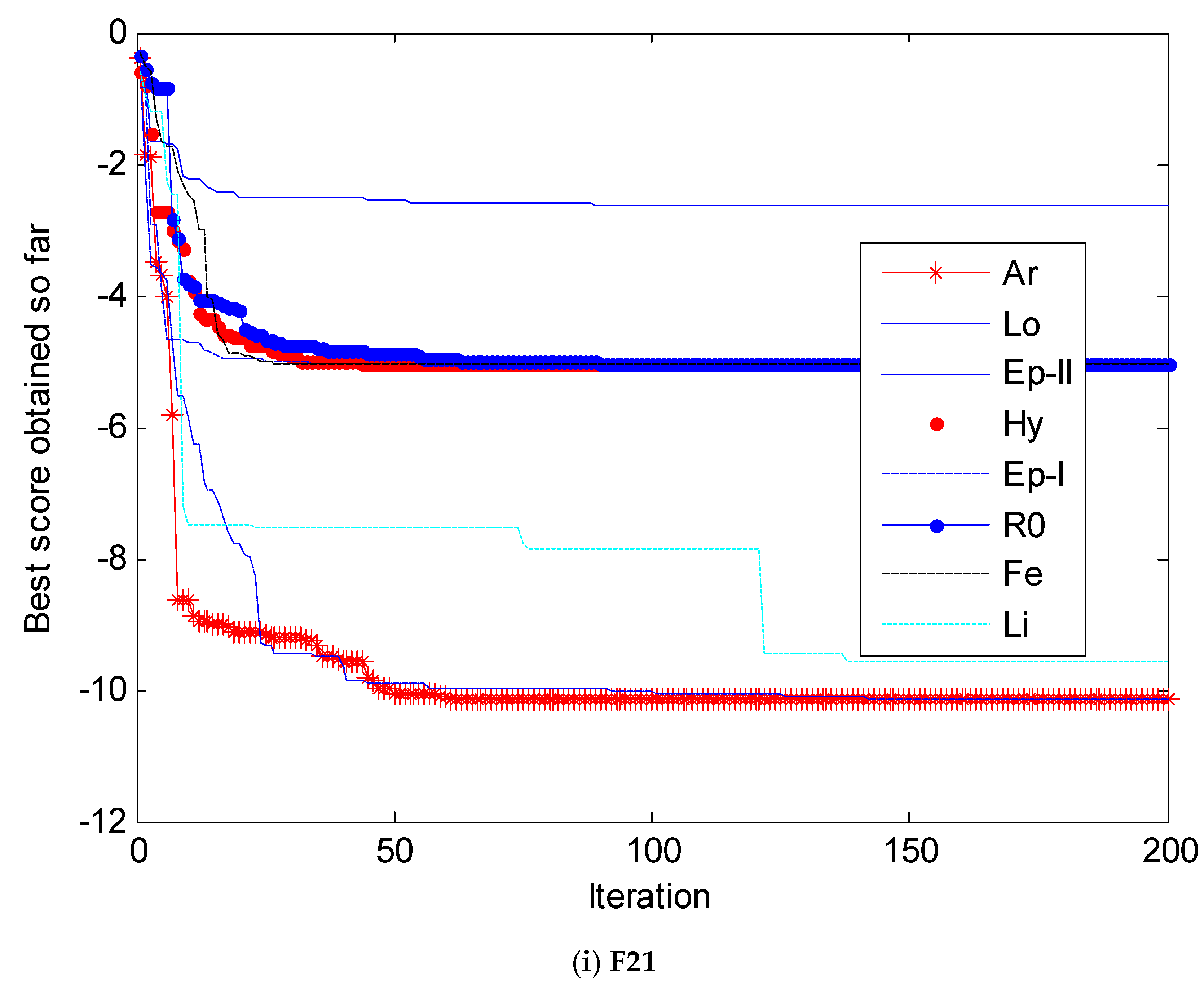
It can be seen from the convergence curves of the benchmark functions and the comparison of the data in Table 2 that in the case of the same number of iterations, the convergence performance of the WOA using the Archimedes spiral curve as the search path of the search agents is superior to the logarithmic spiral curves used in the original algorithm and other seven spiral curves. In particular, for the function F5, F6, F10 and F13, the Archimedes spiral curve makes the convergence speed and accuracy of the algorithm improved obviously compared to other seven helical curves (search paths). Especially for the function F5, this function should be able to converge to 0, but the original WOA can only converge to 27.86, while the convergence of several other swarm intelligent algorithms is not very satisfactory [7]. However, when the search path is changed to the Archimedes spiral curve, the convergence result is obviously close to zero. On the other hand, seen from the three-dimensional images of function F8, F9 and F14, these three functions are very complex multipeak functions, which have many local minimum. In the CP-PDWOA, the added perturbation mechanism can make the algorithm effectively avoid the local minim and search the extreme points, and the convergence speed of the algorithm is obviously improved. It is shown that the improved idea proposed in this paper enhances the ability of the algorithm to avoid the local minimum. From the convergence curves of the functions and the data in Table 2, it can be seen that the improved whale optimization algorithm has excellent search performance.

As can be seen from Figure 15f, when the average value of the function F12 is searched, the areas of the convergence curves corresponding to Lo and Hy are equal, and there is only a slight difference in the early stage. This is not surprising, because from the convergence results of all the models, their convergence results do not think that there are huge differences in other functions; From the paths of the two models, it can be seen that the approximate convergence curve is obtained by adjusting the parameters of the function. The main reason is that these two models fall into the same local extreme point, so we get the same convergence curve, which is also related to the initialization of the agent. Because in order to ensure the feasibility of the simulation, we chose the pseudo-random number as the initial position of the agent.

It is concluded that the introduction of perceptual perturbation not only makes the searching of agents more purposeful, but also makes the location of search agents more diversified and prevents the algorithm from falling into local minim. At the same time, the moving step size of the search agent can be adjusted at different simulation phase so as to ensure that the algorithm in the early search has a strong ability to exploit and in the late search has a stronger explore capability. This ensures the accuracy of the algorithm searching process, but also makes the algorithm have a faster convergence rate.

5. Conclusions

In this paper, we have learned from other scholars’ experience in the improvement of swarm intelligence algorithms, and improved the performance of WOA by introducing disturbance factors. Then the WOA search mechanism is analyzed and the logarithmic spiral curve of equal pitch is used as the search path of the agent. The simulation results also prove that the performance of the equal-pitch Archimedean spiral curve is superior to other types of spiral curve. When collating simulation and algorithm, we found that if we randomly define different search paths for different agents in the same iteration, the resulting convergence performance will be better, but correspondingly, this will also give the algorithm parameters. The adjustment brings a certain degree of difficulty. In summary, the proposed complex path-perceptual disturbance WOA (CP-PDWOA) algorithm has a stronger search performance.

References

- Chandra Mohan, B.; Baskaran, R. A survey: Ant Colony Optimization based recent research and implementation on several engineering domain. Expert Syst. Appl. 2012, 39, 4618–4627. [Google Scholar] [CrossRef]
- Yu, Y.; Li, Y.; Li, J. Nonparametric modeling of magnetorheological elastomer base isolator based on artificial neural network optimized by ant colony algorithm. J. Intell. Mater. Syst. Struct. 2015, 26, 1789–1798. [Google Scholar] [CrossRef]
- Precup, R.E.; Sabau, M.C.; Petriu, E.M. Nature-inspired optimal tuning of input membership functions of Takagi-Sugeno-Kang fuzzy models for anti-lock braking systems. Appl. Soft Comput. 2015, 27, 575–589. [Google Scholar] [CrossRef]
- Vallada, E.; Ruiz, R. A genetic algorithm for the unrelated parallel machine scheduling problem with sequence dependent setup times. Eur. J. Oper. Res. 2011, 211, 612–622. [Google Scholar] [CrossRef] [Green Version]
- Zăvoianu, A.-C.; Bramerdorfer, G.; Lughofer, E.; Silber, S.; Amrhein, W.; Klement, E.P. Hybridization of multi-objective evolutionary algorithms and artificial neural networks for optimizing the performance of electrical drives. Eng. Appl. Artif. Intell. 2013, 26, 1781–1794. [Google Scholar] [CrossRef]
- Kennedy, J. Particle swarm optimization. In Encyclopedia of Machine Learning; Springer: New York, NY, USA, 2010; pp. 760–766. [Google Scholar]
- Yu, Y.; Li, Y.; Li, J. Parameter identification of a novel strain stiffening model for magnetorheological elastomer base isolator utilizing enhanced particle swarm optimization. J. Intell. Mater. Syst. Struct. 2015, 26, 2446–2462. [Google Scholar] [CrossRef]
- Yu, Y.; Li, Y.; Li, J. Forecasting hysteresis behaviours of magnetorheological elastomer base isolator utilizing a hybrid model based on support vector regression and improved particle swarm optimization. Smart Mater. Struct. 2015, 24, 035025. [Google Scholar] [CrossRef]
- Karaboga, D.; Basturk, B. A powerful and efficient algorithm for numerical function optimization: Artificial bee colony (ABC) algorithm. J. Glob. Optim. 2007, 39, 459–471. [Google Scholar] [CrossRef]
- Precup, R.E.; David, R.C.; Petriu, E.M. Grey Wolf Optimizer Algorithm-Based Tuning of Fuzzy Control Systems with Reduced Parametric Sensitivity. IEEE Trans. Ind. Electron. 2016, 64, 527–534. [Google Scholar] [CrossRef]
- Saadat, J.; Moallem, P.; Koofigar, H. Training echo state neural network using harmony search algorithm. Int. J. Artif. Intell. 2017, 15, 163–179. [Google Scholar]
- Vrkalovic, S.; Teban, T.A.; Borlea, L.D. Stable Takagi-Sugeno fuzzy control designed by optimization. Int. J. Artif. Intell. 2017, 15, 17–29. [Google Scholar]
- Reddy, P.D.P.; Reddy, V.C.V.; Manohar, T.G. Whale optimization algorithm for optimal sizing of renewable resources for loss reduction in distribution systems. Renew. Wind Water Solar 2017, 4, 3. [Google Scholar] [CrossRef]
- Trivedi, I.N.; Bhoye, M.; Bhesdadiya, R.H.; Jangir, P.; Jangir, N.; Kumar, A. An emission constraint environment dispatch problem solution with microgrid using Whale Optimization Algorithm. In Proceedings of the Power Systems Conference, Bhubaneswar, India, 19–21 December 2016. [Google Scholar]
- Rosyadi, A.; Penangsang, O.; Soeprijanto, A. Optimal filter placement and sizing in radial distribution system using whale optimization algorithm. In Proceedings of the International Seminar on Intelligent Technology and ITS Applications, Surabaya, Indonesia, 28–29 August 2017; pp. 87–92. [Google Scholar]
- Buch, H.; Jangir, P.; Jangir, N.; Ladumor, D.; Bhesdadiya, R.H. Optimal Placement and Coordination of Static VAR Compensator with Distributed Generation using Whale Optimization Algorithm. In Proceedings of the IEEE 1st International Conference on Power Electronics, Intelligent Control and Energy Systems (ICPEICES), Delhi, India, 4–6 July 2016. [Google Scholar]
- Ladumor, D.P.; Trivedi, I.N.; Jangir, P.; Kumar, A. A Whale Optimization Algorithm approach for Unit Commitment Problem Solution. In Proceedings of the Conference Advancement in Electrical & Power Electronics Engineering (AEPEE 2016), Morbi, India, 14–17 December 2016. [Google Scholar]
- Prakash, D.B.; Lakshminarayana, C. Optimal siting of capacitors in radial distribution network using Whale Optimization Algorithm. Alex. Eng. J. 2016, 56, 499–509. [Google Scholar] [CrossRef]
- Yan, Z.; Sha, J.; Liu, B.; Tian, W.; Lu, J. An Ameliorative Whale Optimization Algorithm for Multi-Objective Optimal Allocation of Water Resources in Handan, China. Water 2018, 10, 87. [Google Scholar] [CrossRef]
- Medani, K.B.O.; Sayah, S.; Bekrar, A. Whale optimization algorithm based optimal reactive power dispatch: A case study of the Algerian power system. Electr. Power Syst. Res. 2017. [Google Scholar] [CrossRef]
- Sun, W.Z.; Wang, J.S. Elman Neural network Soft-sensor Model of Conversion Velocity in Polymerization Process Optimized by Chaos Whale Optimization Algorithm. IEEE Access 2017, 5, 13062–13076. [Google Scholar] [CrossRef]
- Aljarah, I.; Faris, H.; Mirjalili, S. Optimizing connection weights in neural networks using the whale optimization algorithm. Soft Comput. 2016, 22, 1–15. [Google Scholar] [CrossRef]
- Bhesdadiya, R.; Jangir, P.; Jangir, N.; Trivedi, I.N.; Ladumor, D. Training Multi-Layer Perceptron in Neural Network using Whale Optimization Algorithm. Indian J. Sci. Technol. 2016, 9, 28–36. [Google Scholar]
- Wang, J.; Du, P.; Niu, T.; Yang, W. A novel hybrid system based on a new proposed algorithm—Multi-Objective Whale Optimization Algorithm for wind speed forecasting. Appl. Energy 2017, 208, 344–360. [Google Scholar] [CrossRef]
- Niu, P.F.; Wu, Z.L.; Ma, Y.P.; Shi, C.J.; Li, J.B. Prediction of steam turbine heat consumption rate based on whale optimization algorithm. CIESC J. 2017, 68, 1049–1057. [Google Scholar]
- Aziz, M.A.E.; Ewees, A.A.; Hassanien, A.E. Whale Optimization Algorithm and Moth-Flame Optimization for multilevel thresholding image segmentation. Expert Syst. Appl. 2017, 83, 242–256. [Google Scholar] [CrossRef]
- Mostafa, A.; Hassanien, A.E.; Houseni, M.; Hefny, H. Liver segmentation in MRI images based on whale optimization algorithm. Multimed. Tools Appl. 2017, 76, 24931–24954. [Google Scholar] [CrossRef]
- Jangir, P.; Jangir, N. Non-Dominated Sorting Whale Optimization Algorithm (NSWOA): A Multi-Objective Optimization Algorithm for Solving Engineering Design Problems. Glob. J. Res. Eng. 2017, 17, 15–42. [Google Scholar]
- Oliva, D.; Aziz, M.A.E.; Hassanien, A.E. Parameter estimation of photovoltaic cells using an improved chaotic whale optimization algorithm. Appl. Energy 2017, 200, 141–154. [Google Scholar]
- Sharawi, M.; Zawbaa, H.M.; Emary, E. Feature selection approach based on whale optimization algorithm. In Proceedings of the Ninth International Conference on Advanced Computational Intelligence, Doha, Qatar, 4–6 February 2017; pp. 163–168. [Google Scholar]
- Zhao, G.; Zhou, Y.; Ouyang, Z.; Wang, Y. A Novel Disturbance Parameters PSO Algorithm for Functions Optimization. Adv. Inf. Sci. Serv. Sci. 2012, 4, 51–57. [Google Scholar]
- Jing, Y.E. The Diversity Disturbance PSO Algorithm to Solve TSP Problem. J. Langfang Teach. Coll. 2010, 5, 2. [Google Scholar]
- Li, D.; Deng, N. An electoral quantum-behaved PSO with simulated annealing and gaussian disturbance for permutation flow shop scheduling. J. Inf. Comput. Sci. 2012, 9, 2941–2949. [Google Scholar]
- Gao, H.; Kwong, S.; Yang, J.; Cao, J. Particle swarm optimization based on intermediate disturbance strategy algorithm and its application in multi-threshold image segmentation. Inf. Sci. 2013, 250, 82–112. [Google Scholar] [CrossRef]
- Mirjalili, S.; Lewis, A. The Whale Optimization Algorithm. Adv. Eng. Softw. 2016, 95, 51–67. [Google Scholar] [CrossRef]
- Mafarja, M.M.; Mirjalili, S. Hybrid Whale Optimization Algorithm with simulated annealing for feature selection. Neurocomputing 2017, 260, 302–312. [Google Scholar] [CrossRef]
- Ling, Y.; Zhou, Y.; Luo, Q. Lévy Flight Trajectory-Based Whale Optimization Algorithm for Global Optimization. IEEE Access 2017, 5, 6168–6186. [Google Scholar] [CrossRef]
- Abdel-Basset, M.; El-Shahat, D.; El-Henawy, I.; Sangaiah, A.K.; Ahmed, S.H. A Novel Whale Optimization Algorithm for Cryptanalysis in Merkle-Hellman Cryptosystem. Mob. Netw. Appl. 2018, 5, 1–11. [Google Scholar] [CrossRef]
- Kaveh, A.; Ghazaan, M.I. Enhanced Whale Optimization Algorithm for Sizing Optimization of Skeletal Structures. Mech. Based Des. Struct. Mach. 2017, 45, 345–362. [Google Scholar] [CrossRef]
- Spiral Curve. Van Nostrand’s Scientific Encyclopedia; John Wiley & Sons, Inc.: Hoboken, NJ, USA, 2005. [Google Scholar]
- Ren, Y.; Wu, Y. An efficient algorithm for high-dimensional function optimization. Soft Comput. 2013, 17, 995–1004. [Google Scholar] [CrossRef]
- Yuan, Z.; de Oca, M.A.M.; Birattari, M.; Stützle, T. Continuous optimization algorithms for tuning real and integer parameters of swarm intelligence algorithms. Swarm Intell. 2012, 6, 49–75. [Google Scholar] [CrossRef]
Figure 1.
Theoretical basis of two-dimensional plane.
Figure 2.
Figure 3.
Theoretical basis of shrinking encircling mechanism.
Figure 4.
Sketch map of spiral renewal position method.
Figure 5.
Two-dimensional curve of Logarithmic spiral.
Figure 6.
Two-dimensional curve of equal pitch Archimedes spiral.
Figure 7.
Two-dimensional curve of a Rose spiral with four leaves.
Figure 8.
Two-dimensional curve of Epicycloid-I.
Figure 9.
Two-dimensional curve of Hypotrochoid.
Figure 10.
Two-dimensional curve of Epicycloid-II.
Figure 11.
Two-dimensional curve of Fermat spiral.
Figure 12.
Two-dimensional curve of Lituus spiral.
Figure 13.
Three-dimensional images of some optimization functions.
Figure 14.
Comparison of the convergence curves of the partial functions to verify disturbances.
Figure 15.
Comparison of the convergence curves of the partial functions.