Intelligent Prognostics of Degradation Trajectories for Rotating Machinery Based on Asymmetric Penalty Sparse Decomposition Model


1
College of Mechanical Engineering, Donghua University, Shanghai 201620, China
2
George W. Woodruff School of Mechanical Engineering, Georgia Institute of Technology, Atlanta, GA 30332-0405, USA
*
Author to whom correspondence should be addressed.
Symmetry 2018, 10(6), 214; https://doi.org/10.3390/sym10060214
Submission received: 22 May 2018
/
Revised: 7 June 2018
/
Accepted: 8 June 2018
/
Published: 12 June 2018
(This article belongs to the Special Issue Symmetry and Complexity)
Abstract
:The ability to accurately track the degradation trajectories of rotating machinery components is arguably one of the challenging problems in prognostics and health management (PHM). In this paper, an intelligent prediction approach based on asymmetric penalty sparse decomposition (APSD) algorithm combined with wavelet neural network (WNN) and autoregressive moving average-recursive least squares algorithm (ARMA-RLS) is proposed for degradation prognostics of rotating machinery, taking the accelerated life test of rolling bearings as an example. Specifically, the health indicators time series (e.g., peak-to-peak value and Kurtosis) is firstly decomposed into low frequency component (LFC) and high frequency component (HFC) using the APSD algorithm; meanwhile, the resulting non-convex regularization problem can be efficiently solved using the majorization-minimization (MM) method. In particular, the HFC part corresponds to the stable change around the zero line of health indicators which most extensively occurs; in contrast, the LFC part is essentially related to the evolutionary trend of health indicators. Furthermore, the nonparametric-based method, i.e., WNN, and parametric-based method, i.e., ARMA-RLS, are respectively introduced to predict the LFC and HFC that focus on abrupt degradation regions (e.g., last 100 points). Lastly, the final predicted data could be correspondingly obtained by integrating the predicted LFC and predicted HFC. The proposed methodology is tested using degradation health indicator time series from four rolling bearings. The proposed approach performed favorably when compared to some state-of-the-art benchmarks such as WNN and largest Lyapunov (LLyap) methods.
1. Introduction
Rotating machines are critical elements of almost all forms of mechanical assemblies, which play an important role in today’s industrial applications. Unexpected failures and unscheduled system interruptions caused by harsh working environments may result in costly lapse in production or even catastrophic incidents. Accurate/timely prediction and health assessment of rotating machines are of great significance in the functionality and performance of these equipment, especially in the early stages of failure [1,2,3].
Accordingly, in recent years, a plethora of research works have proposed tracking the degradation trend of rotating machines and predicting their remaining useful life (RUL), wherein condition-based prognostics maintenance (CBPM) has become an efficient strategy for the PHM of rotating machines. The CBPM is based on the data information collected via embedded sensors to assess and judge the real-time state of the mechanical assemblies, and then predict their degradation trend to develop appropriate decisions on maintenance activities before failure occurs. More advanced prognostics techniques are focused on degradation assessment of the systems, but it is also a relatively complex problem due to the non-stationary and nonlinear characteristic of data information [4,5,6]. Generally, to fulfill the goal of prognostics, three crucial steps are needed:
- (1)
- The historical data with long-terms, including normal and abnormal time series data, should be collected using sensors and other portable testing devices. Typically, good degradation data must capture the physical transitions that the rotating machinery such as rolling bearing undergo during different stages of its running life; fortunately, most of the historical data are easy to collect since the rotating machinery is frequently updated in real time.
- (2)
- The health indicators (e.g., peak-to-peak value and Kurtosis) should be extracted to assess and continuously track the health condition of rotating machines or system. The health indicators are used to design a suitable prediction model that captures the evolution of the degradation trend of rotating machines.
- (3)
- The reliable prediction models and possible failure models should be established and the remaining useful life (RUL) or future trajectory of rotating machines could be effectively predicted.
Among these three steps, model establishment and trajectory estimation are the most important and challenging steps because of the stochastic nature and nonlinear characteristics of the health indicators. Therefore, many researchers have laid their emphasis on model foundation in recent years. From the view of application, roughly, the existing prediction approaches can be divided into two categories: (a) parametric-based methods and (b) nonparametric-based methods. In the literature, parametric-based methods mainly include time-series methods such as autoregressive moving average (ARMA) [7,8], fractional autoregressive integrated moving average (FARIMA) [9,10], fractional Brownian motion (FBM) [11,12], hidden Markov model (HMM) [13,14] and grey theoretical model (GTM) [15,16], etc. Generally, the parametric-based methods overcome the hurdle of predictive availability during long-term prediction (according to needs) which assumes the model’s parameters to be constants in the predicted region. However, due to the stochastic, complex and nonlinear properties of health indicators time series (HITS), the trade-off of parametric-based method is that only accurate prediction with real-time can help adjust the system model. Otherwise, the prediction performance may not be ensured. In addition, the parametric-based methods are often developed case by case, thus model parameters identification also requires extensive experiments, and therefore, it is usually not desirable in practice.
To address this issue, much attention has recently been focused on the nonparametric-based methods in the degradation prognostic of rotating machinery. For instance, artificial neural network (ANN) [17,18,19,20], fuzzy logic [21], and deep learning network (DPN) [22,23], etc., could be considered as successful nonparametric-based approaches in the PHM field. The benefit of using nonparametric-based methods lies in their ability to model the evolution of complex multi-dimensional degradation data, which can effectively extract latent features such as the spatio-temporal correlations (STC) among historical data. In addition, for the nonparametric-based methods, it is not necessary to establish an accurate linkage between the reliability health indicators and physical degradation such as crack propagation in an individual element. However, the common drawbacks associated with these nonparametric-based techniques are time-consuming and a large number of training samples are required in advance.
Due to time-variant and non-stationary characteristics of the health indicators, and the disadvantages of the model, which is sometimes case-specific, it is difficult to determine the best prognostic model. Therefore, it is intuitive to develop a fusion idea via combining parametric-based methods and nonparametric-based methods to blend their merits and enhance the prediction performance of degradation trajectories. However, it is not clear how to fuse parametric-based and nonparametric-based models to improve the prediction accuracy, especially when health indicators become abundant and redundant.
It is generally thought that the health indicators time series (HITS) is commonly composed of different sub-components which correspond to different time-variant characteristics of the systems. In this work, we assume that the HITS is mainly composed of high frequency component (HFC) and low frequency component (LFC). The HFC part corresponds to the stable change around the zero line of the HITS which frequently occurs; in contrast, the LFC part is essentially related to the evolutionary trend of the HITS which rarely occurs in practice, because the stable running trend occupies most of the life time, only the drastic trend can be clearly emerged when the failures are serious. This can be explained using degradation trajectories of several rotating machines (e.g., rolling bearings) as shown in Figure 1, where the degradation process of the bearings generally consists of two phases, i.e., phase I: the normal operation phase and phase II: the failure phase. The degradation health indicator in phase I is stable, which means that the bearing is normal. The degradation process changes from phase I to phase II once a fault occurs, where the HITS generally increases as the fault gets worse, the curve that rises steadily could be assumed as the LFC; in contrast, the volatile components with large and small amplitude could be treated as the HFC. To ensure better prediction accuracy, it is necessary to isolate the LFC associated with bearing defects and HRC associated with structural vibration from the degradation trajectories, and then develop a degradation algorithm based on both components.
To overcome this problem, a sparse low-rank matrix decomposition (SLMD) method is introduced in this research. In recent years, many researchers have laid their emphasis on fault diagnosis and sparse filtering using SLMD algorithm. For instance, in ref. [24], Selesnick et al. developed a convex low-rank matrix decomposition approach based on non-convex bivariate penalty function for sparse one-dimensional deconvolution. In ref. [25], He et al. proposed convex sparsity-based regularization scheme to extract multiple faults of motor bearing and locomotive bearing. In refs. [26,27], Li et al. proposed a bicomponent sparse low-rank matrix separation and group sparsity total variation de-noising approach to extract transient fault impulses from the noisy vibration signals, using the rolling bearing and gearbox as example. In ref. [28], Wang et al. utilized a sparse low-rank matrix decomposition method based on generalized minimax-concave (GMC) penalty to explore and diagnosis the localized faults in rolling bearings. In refs. [29,30], Parekh et al. proposed an enhanced low-rank matrix approximation and its effectiveness was verified by the synthetic data and nonlocal self-similarity based image. In ref. [31], Ding et al. proposed the sparse low-rank matrix decomposition (SLMD) algorithm based on split augmented Lagrangian shrinkage (SALS) algorithm with majorization-minimization (MM) to detect and extract the periodical oscillatory features of gearbox of an oil refinery.
Unfortunately, despite the effectiveness of the above approaches, the SLMD approaches still suffer from the following several challenges and their application development has been restricted:
- (1)
- Generally, the penalty functions that are established in a low-rank matrix approximation model are symmetric function, e.g., absolute value function; the common drawback is that this penalty function is non-differentiable at zero point, which can lead to some numerical issues such as local optimum and early termination of algorithm.
- (2)
- In conventional SLMD methods, the convex regularizer (e.g., L1-norm) which usually underestimates the sparse signal when the absolute value function is used as a sparsity regularizer. Additionally, both the convex and nonconvex methods shrink all the coefficients equally and remove too much energy of useful information, resulting in the separation of the LFC and HFC becoming more challenging.
To overcome these limitations and to robustly separate the LFC and HFC from degradation trajectories of health indicators, a novel asymmetric penalty sparse decomposition (APSD) algorithm with non-convex sparsity constraint is proposed in this work. The resulting non-convex regularization problem will be efficiently handled using the majorization-minimization (MM) method. Having the LFC and HFC separated, the LFC and HFC components (e.g., last 100 points) will be predicted using the wavelet neural network (WNN) and ARMA combined with recursive least squares algorithm (ARMA-RLS) methods, respectively. In an effort to establish a comprehensive assessment of degradation processes, the proposed fusion prognostics framework combines the WNN (a nonparametric-based approach) and the ARMA-RLS (a parametric-based approach) in an attempt to improve the prediction performance, in which the physical information of the degenerative process and massive sample data are not considered and accommodated. The final predicted data could be generated by combining the predicted LFC and HFC components. Finally, we demonstrate the proposed approach by four case studies of accelerated aging tests of rolling bearing.
The main contributions of this paper are summarized as follows:
- (1)
- To address the issue of models merging and improve the prediction accuracy, the health indicators time series (HITS) is decomposed into different sub-components, i.e., low frequency component (LFC) and high frequency component (HFC), using the APSD algorithm.
- (2)
- To address the drawback that penalty function is non-differentiable at zero point, a new asymmetric penalty function is proposed.
- (3)
- To solve the proposed non-convex regularization problem based on asymmetric penalty function, the majorization-minimization (MM) algorithm is introduced.
- (4)
- The decomposed LFC and HFC components can be predicted using the wavelet neural network (WNN) and ARMA combined with recursive least squares algorithm (ARMA-RLS) methods, respectively.
- (5)
- The prediction accuracy is greatly improved compared with some state-of-the-art models, and the presented approach has powerful application potentials.
The frame of this paper is structured as follows. Section 2 contains the description of the asymmetric nonconvex sparse decomposition (APSD) algorithm. Section 3 provides the algorithms of degradation modeling, i.e., wavelet neural network and ARMA combined with recursive least squares algorithm (ARMA-RLS) methods. Experimental results and discussion are given in Section 4. Finally, Section 5 concludes with a discussion of future research.
2. Asymmetric Penalty Sparse Decomposition (APSD) Algorithm
2.1. Sparse Representation and Filter Banks
Generally, the fault vibration signal (observation signal) y of rotating machinery such as rolling bearing, which contains three parts below: the fault transient impulses x, the systematic natural signal f and the additive noise w, i.e.,
The core work of the fault diagnosis is to extract the fault transient impulses x from the noisy observation y. Assume that fault transient impulses and the systematic natural signal are estimated, we have,
Given an estimation of x, we can estimate f as follows,
where LPF is a specified low-pass filter. Substituting into , we have,
Substituting into , we have,
Substituting into , we have,
Defining HPF = I − LPF = H, which is a high-pass filter, thus we have,
On the other hand, it should be noted that Equation (1) is a highly underdetermined equation, i.e., ill-posed or N − P hard problem [32,33], and has an infinite set of solutions because the number of unknowns is greater than the number of equations. Usually, convex optimization techniques are commonly used to estimate transient components from the observation signal, based on the aforementioned work [24,25,26,27,28,29,30,31], the estimation of x can be formulated as the optimization problem, i.e.,
where H is a specified high-pass filter, i.e., the HPF in Equation (7), λ represents regularization term parameter, D is a matrix defined as , which determines the sparsity degree of the approximating value of x. Commonly, if x is a sparse component, i.e., most of the values in x tend to zero, the correspondingly optimization problem in Equation (8) can be estimated by L1-norm fused lasso optimization (LFLO) model [24,25,26,27,28,29,30,31], i.e.,
where λ0 and λ1 are regularization parameters. The solution of LFLO model can be obtained by the soft-threshold method [34] and total variation de-noising (TVD) algorithm [35,36,37], we have,
where function is the TVD algorithm and the soft-threshold model is given as follows,
2.2. Asymmetric Penalty Regularization Model
Compare with optimization algorithm Equations (8) and (9), to estimate the fault transient impulses x precisely, this work introduces a novel penalty regularization method, i.e., asymmetric and symmetric nonconvex penalty regularization model,
where F(x) is the proposed objective cost function (OCF), penalty function is a asymmetric and differentiable function, and is a symmetric and differentiable function, if term M = 2, matrix D1 defined as , and matrix D2 defined as . The innovations of the novel compound regularizer model are as follows:
- (I)
- The M-term compound regularizers to estimate the fault transient impulses;
- (II)
- The compound regularizer model consists of symmetric and asymmetric penalty functions, wherein the symmetric penalty function is a differentiable function compared with the nondifferentiable function at point i = 0.
- (III)
- The MM algorithm is introduced for the solution of proposed compound regularization method, i.e., the OCF.
Based on this, the core issues of the proposed algorithm are (1) how to construct a symmetric and differentiable penalty function; (2) how to construct an asymmetric and differentiable penalty function and; (3) how to solve the proposed method based on the MM algorithm and make diagnosis results are more accurate than the traditional LFLO and nonconvex penalty regularization approaches.
For the first issue, traditional LFLO regularization approach uses the absolute value function as the penalty function; however, the common drawback of function is that this function is non-differentiable at zero point, which can cause some numerical problems. To address this problem, a non-linear approximation function of or is proposed, i.e.,
Note that when , then the and degrade into the absolute value function , while the , the and are differentiable at zero point. The function , , and their first-order derivatives are listed in Table 1.
In order for the non-linear approximation functions to maintain the reliable sparsity-inducting behavior of the original LFLO algorithm, the parameter should be presented to an adequately small positive value. Fortunately, for example, the parameter and which are small enough so that the numerical issues can be avoided.
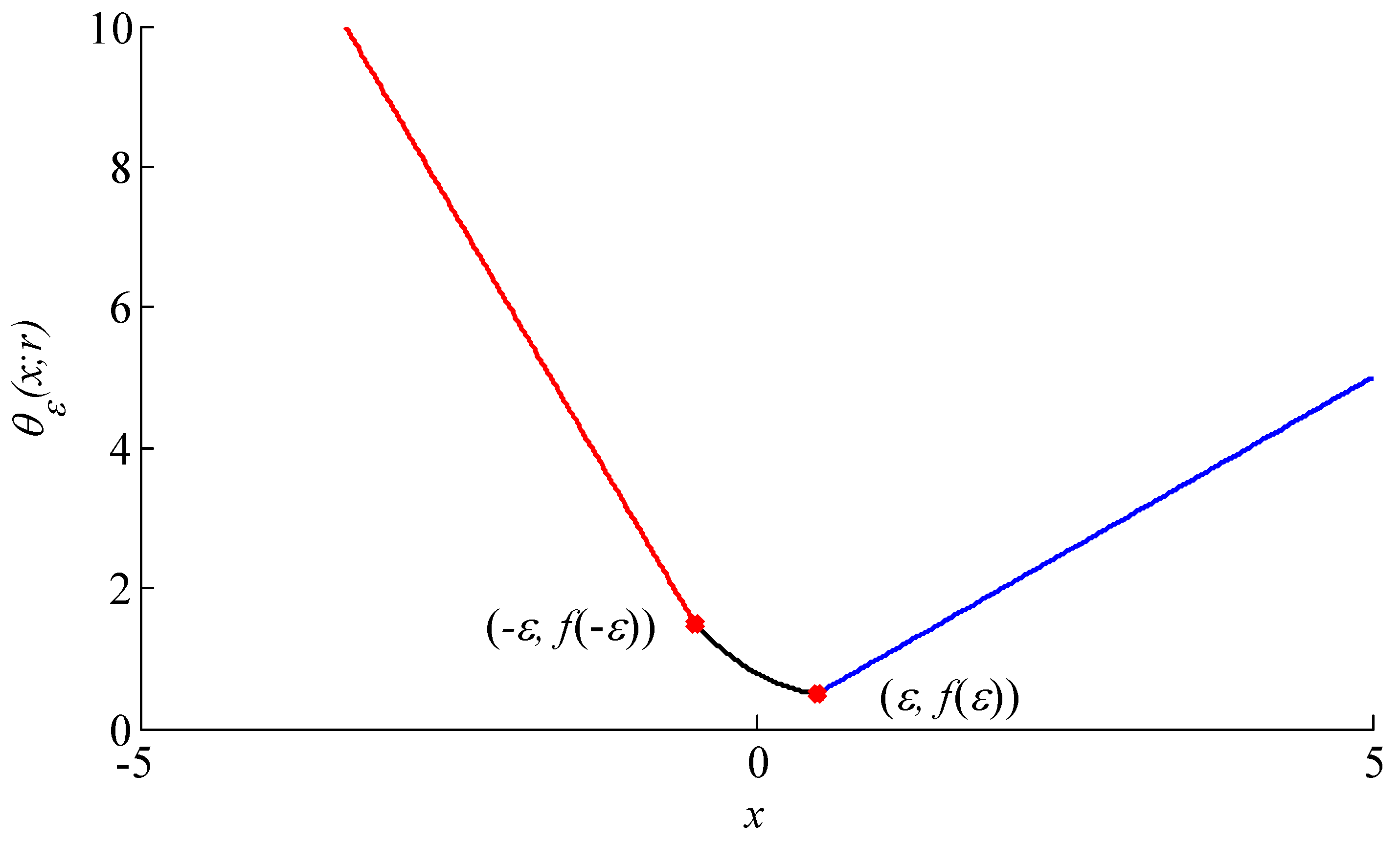
For the second issue, inspired by the absolute value function , and also in contrast to the symmetric and differentiable penalty function and , here, a segmented function is proposed as follows,
where is a positive constant. It should be noted that if we exclude the intermediate function f(x), the is also degrade into the absolute value function when r = 1. Therefore, the main problem of Equation (16) will transform into a task of how to construct the intermediate function . To address this issue, we seek a majorizer (here the Majorization-minimization algorithm is utilized) as the approximation function of . In order to eliminate the issue that penalty function is non-differentiable at zero point, a simple quadratic equation (QE) is introduced accordingly,
The parameter a, b, c and s are all functions of v, we have,
Substituting Equation (19) into , we have,
Similarly, the numerical issue of Equation (20) will appear if the parameter v approaches zero. To address this problem, the sufficiently small positive value is used instead of , thus, the segmented function Equation (16) can be rewritten as,
Hence, the new function is a continuously differentiable function. The plot of the continuously differentiable asymmetric penalty function is shown in Figure 2, and the function is a second-order polynomial on .
The third issue, will be solved and derived in Section 2.3 using the majorization-minimization algorithm.
2.3. The Solution of Proposed Model Based on Majorization-Minimization Algorithm
In this paper, the majorization-minimization (MM) algorithm is implemented to derive an iterative solution procedure for the proposed approach [38]. The G(x,v) is chosen as the majorizer of F(x). Specifically, the iterative solution procedure could be divided into three phases:
- (a)
- Majorizer of symmetric and differentiable function based on MM algorithm.
- (b)
- Majorizer of asymmetric and differentiable function based on MM algorithm.
- (c)
- Majorizer of objective cost F(x) based on MM algorithm.
For problem (a), we first seek a majorizer for , i.e.,
Since is symmetric function, we set to be an even second-order polynomial, i.e.,
Thus, according to Equation (22) and and , we have,
The parameter m and b can be computed as,
Substituting Equation (25) in Equation (23), we have
Summing, we obtain,
where is diagonal matrix and .
Therefore, based on Equation (27), we obtain,
where is diagonal matrix and .
For problem (b), assume that is the majorizer of the asymmetric and differentiable function , since the , we have,
when , then,
when , then,
Therefore, the majorizer of the asymmetric and differentiable function is obtained,
Summing, we obtain,
where is a diagonal matrix, i.e., and , and .
For problem (c), based on Equations (28) and (33), the majorizer of F(x) based on MM algorithm is given by,
Minimizing G(x,v) with respect to x yields,
Substituting H = BA−1 in Equation (35), we have,
where matrix and matrix .
Finally, by using the above formulas, the fault transient impulses x can be obtained by the following iterations,
In conclusion, the complete steps of the proposed algorithm are summarized as follows,
- (1)
- Inputs: signal y, r ≥ 1, matrix A, matrix B, , k = 0;
- (2)
- (3)
- Initialize x = y;
- (4)
- Repeat the following iterations:
- (5)
- If the stopping criterion is satisfied, then output signal x, otherwise, k = k + 1, and go to step (4).
- (6)
- Output: signal x.
2.4. Parameters Selection
In this section, the regularization parameters λi are set as [26]:
where β0 and β1 are the constants so as to maximize the signal-to-noise-rate (SNR), β0 and γ are typically set up to be constants, i.e., β0 = [0.5, 1], γ = [7.5, 8], and σ is the standard deviation (SD) of the external noise. In practical engineering applications, the SD of the external noise in Equation (40) could be computed using the healthy data and fault data under the same operating environment. Moreover, when the healthy data is not available or unknown, the SD of the external noise can still be estimated by the following formula,
where the Equation (41) is a noise level estimator that used for traditional wavelet denoising in ref. [41], and MAD(y) represents the median absolute deviation (MAD) of observation signal y, i.e.,
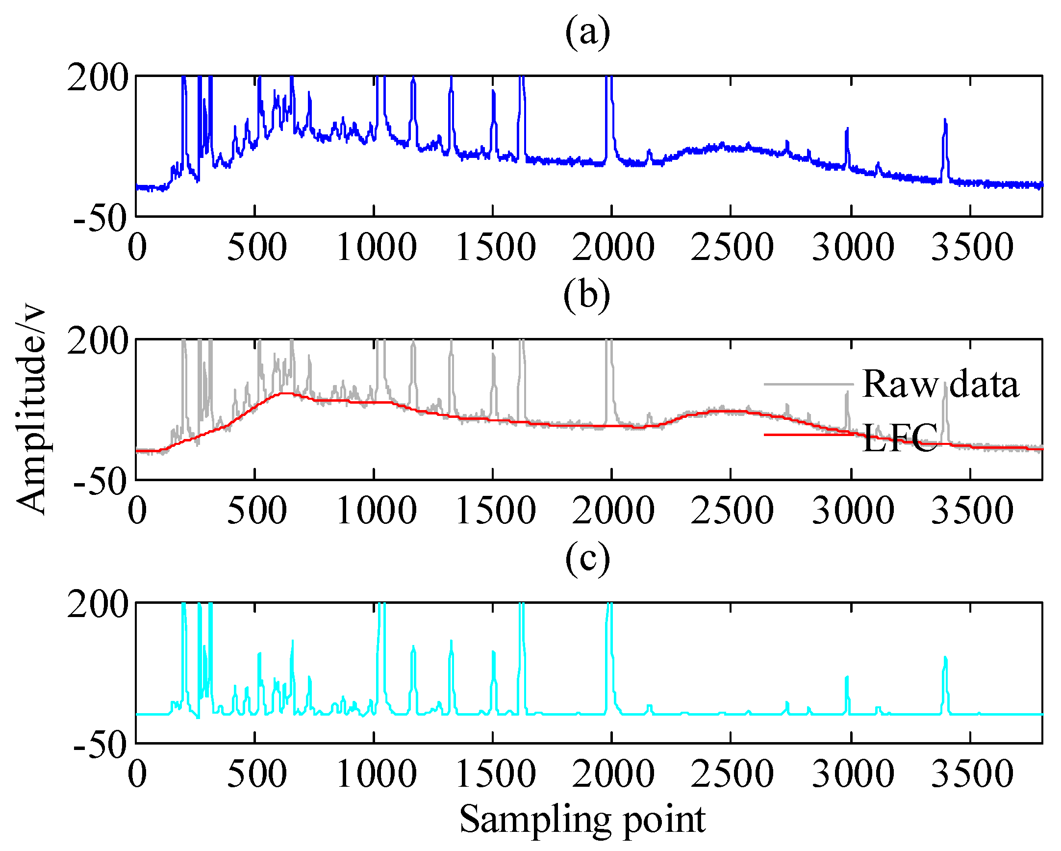
To better understand the asymmetric penalty sparse decomposition algorithm, a chromatogram signal is analyzed by the proposed APSD algorithm [38]. For illustration, Figure 3a exhibits the raw chromatogram signal. Figure 3b,c respectively shows the LFC and HFC that generated by the proposed APSD. Note that the main evolutionary trend, i.e., low frequency component, is well estimated as illustrated in Figure 3b, meanwhile, the estimated peaks, i.e., high frequency component, illustrated in Figure 3c, are well delineated. Therefore, the LFC and HFC components could be captured by the asymmetric penalty sparse decomposition algorithm.
3. Wavelet Neural Network and ARMA-RLS Algorithm
3.1. Wavelet Neural Network Algorithm
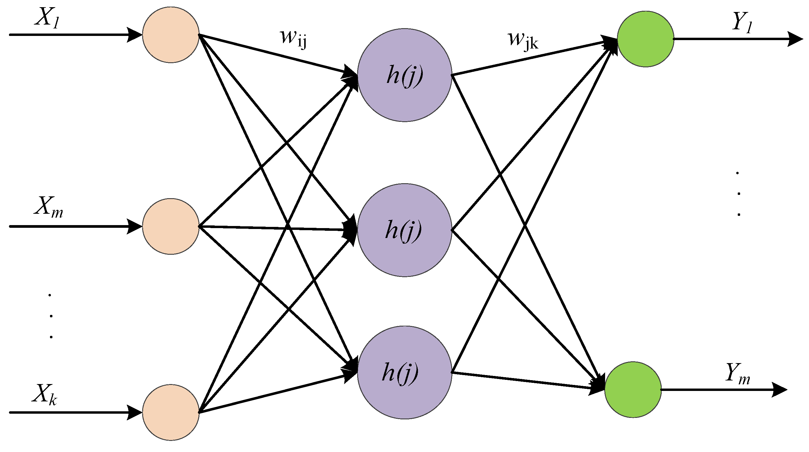
Wavelet neural network (WNN) is a recently developed neural network with a topology and structure that are similar to that of the back-propagation neural network (BPNN) [42,43,44,45]. The network structure is composed of the input layer, hidden layer and output layer; the topology structure of the WNN is shown in Figure 4, wherein the customary sigmoid function (CSF) is replaced by the wavelet basis functions h(j) as activation function for the neurons in hidden layer. Hence, the combination of wavelet transform and BPNN has the advantage of both wavelet analysis and neural network; the data is transmitted forward and the prediction error is propagated backward, so as to achieve a more accurate predictive data.
Generally, prediction accuracy and generalization ability will be affected by the choice of wavelet base function; compared to orthogonal wavelet, Gauss spline wavelet and Mexico hat wavelet, the Morlet wavelet has the smallest error and the reliable computational stability [46,47], thus this study employed Morlet wavelet as the activation function of hidden layer nodes, the formula is given below,
In Figure 4, the input data are represented by X1, X2, …, Xk, and the predicted outputs are denoted by Y1, Y2, …, Ym, wij is the link-weight between the input layer and hidden layer. When the input data is xi (i = 1, 2, …, k), the output of hidden layer can be calculated as,
where h(j) is the output of the j-th hidden layer and also represents the wavelet basis function, aj is the scaling factor of function h(j), bj is the translation factor of function h(j), The output of the WNN can be expressed as,
where wik denotes the link-weight between the hidden layer and output layer, h(i) is the output of the i-th hidden layer, l represents the number of hidden layer and m represents the number of output layer. According to the fundamental principle of BPNN and gradient descent learning algorithm, the corresponding adjustment process of network weights and wavelet basis function is as follows,
(1) Calculate network prediction error, i.e.,
where yn(k) is desired outputs and y(k) predicted outputs generated by the WNN method.
(2) network weights and wavelet basis function can be adjusted by network prediction error, i.e.,
where the parameters , and could be calculated as follows,
where η is learning rate. The training and correcting algorithm steps of the network parameters are as follows:
Step 1: Network initialization. The expansion parameters ak and translation parameters bk of the wavelet basis function as well as the network learning rate η, the link-weights are wij and wjk, respectively, the error threshold ε, and maximum iterations T.
Step 2: Samples classification. Samples can be divided into training samples and test samples, wherein the training samples are applied for network training and the test samples are applied for testing prediction accuracy.
Step 3: Predicted output. The training samples are feed into the WNN network, and the predicted outputs are calculated. Then the error and gradient vectors of the output of WNN and the desired output are obtained.
Step 4: Weights adjustment. The parameters of the wavelet basis function and the back propagation of error corrects the weights of the WNN.
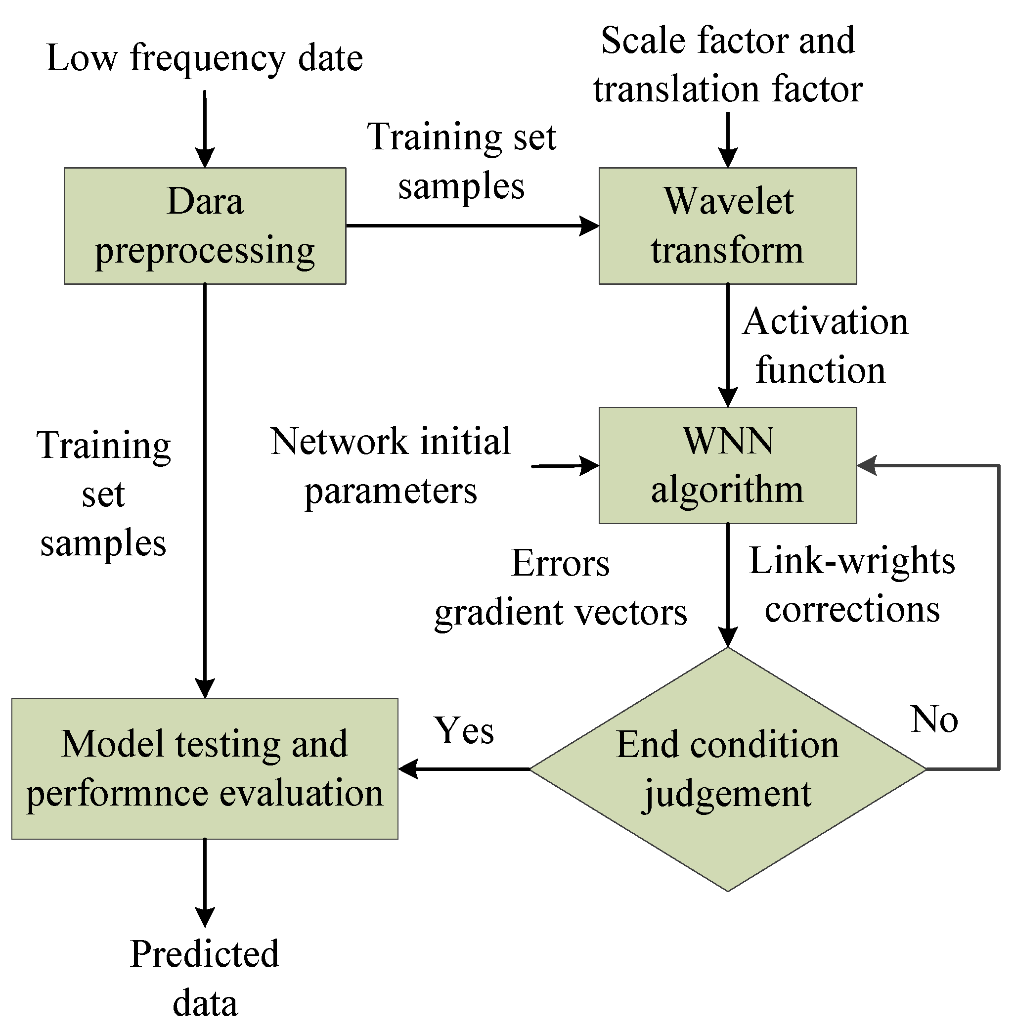
Step 5: End conditions. The training algorithm will judge whether the targeted error is less than the predetermined threshold ε (ε > 0) or exceeds the maximum iterations. If yes, the network training is stopped, otherwise, the algorithm returns to step 3. The training and correcting steps of the WNN are shown in Figure 5.
3.2. ARMA Combined With Recursive Least Squares (RLS) Algorithm
3.2.1. ARMA Review of ARMA Model
A stochastic process Xt is called an autoregressive moving-average process (ARMA) with order p and q, namely ARMA (p, q) [48,49], if the process is stationary and satisfies a linear stochastic difference equation of the form,
where et is white gaussian noise (WGN), i.e., , parameters and are coefficients of AR(p) and MA(q) models, and the polynomials are as follows,
3.2.2. Recursive Least Squares (RLS) Algorithm
Given an input samples set and a desired response set , the output y(n) could be computed by linear filter method as follows,
Minimizing the sum of the error squares, we have,
where the error e(i) is , and the is the forgetting factor and . To simplify the writing format, taking the form as . Thus, the sum of error squares can be rewritten as,
Defining the following formulas,
Then the Equation (58) can be rewritten as,
which is the standard least squares (LS) criterion, the solution of the LS can be obtained as,
where parameters and . Based on , thus the at time n − 1 could be obtained, i.e.,
Therefore, the variables and can be rewritten using and , i.e.,
and
The matrix inversion formula of is as follows,
Denoting
and
Therefore,
The main time-update equation can be derived as,
where is the innovation process. In conclusion, the prediction processes of the ARMA combined with RLS algorithm are summarized as follows,
Step 1: Algorithm initialization. The forgetting factor , the predicted steps n.
Step 2: Initial parameter calculation. Calculate the initial order p and q of ARMA (p, q) model using Akaike information criterion (AIC) [50] based on historical data.
Step 3: Coefficients extraction. Extract the coefficients and as the input u(i) of RLS algorithm, i.e., .
Step 4: Prediction iteration based on RLS algorithm. Repeat the following iterations,
Step 5: Judgment of the end conditions. If the iterative step is satisfied, then output predicted signal y(n), otherwise, i = i + 1, and go to step (4).
4. Experimental Validations
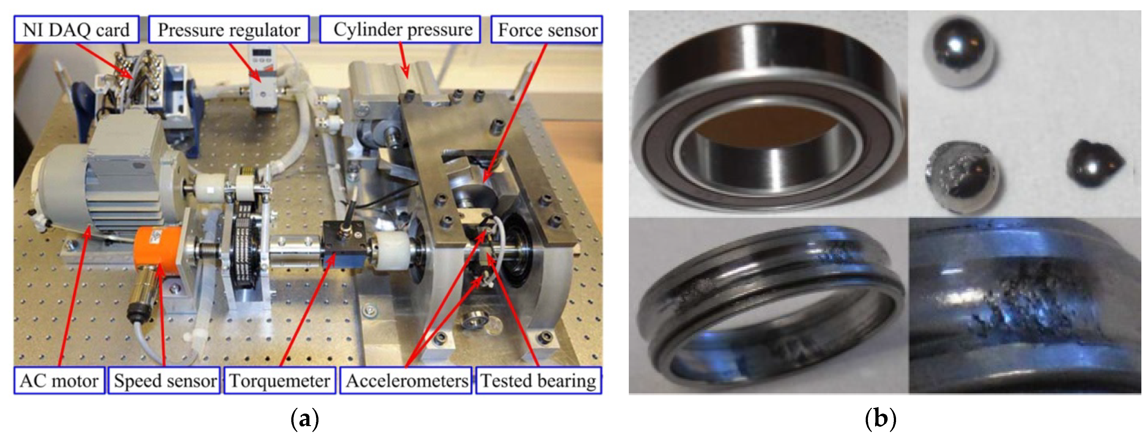
The vibration data collected from accelerated life tests (ALT) of rolling bearings were employed to validate the effectiveness of the proposed approach, the experimental setup is shown in Figure 6a. The experimental data were acquired and published by the IEEE-PHM Association [51,52]. The experimental platform included National Instruments (NI) data acquisition card, pressure regulator, cylinder pressure, force sensors, motor, speed sensor, torque-meter, accelerometers and tested bearing, etc. During the process of the experiment, the rotating speeds of the bearing were set to 1650 r/min and 1800 r/min, and 17 bearings were chosen during all those experiments. The sampling frequency was 25.6 kHz, and 2560 sample points (i.e., 0.1 s) were recorded each 10 s. The experimental tests were stopped if the amplitude of time-domain data exceeded 20 g. As shown in Figure 6b, the severe wear in bearing elements and the severe spalling failure in inner race were observed after dismantling.
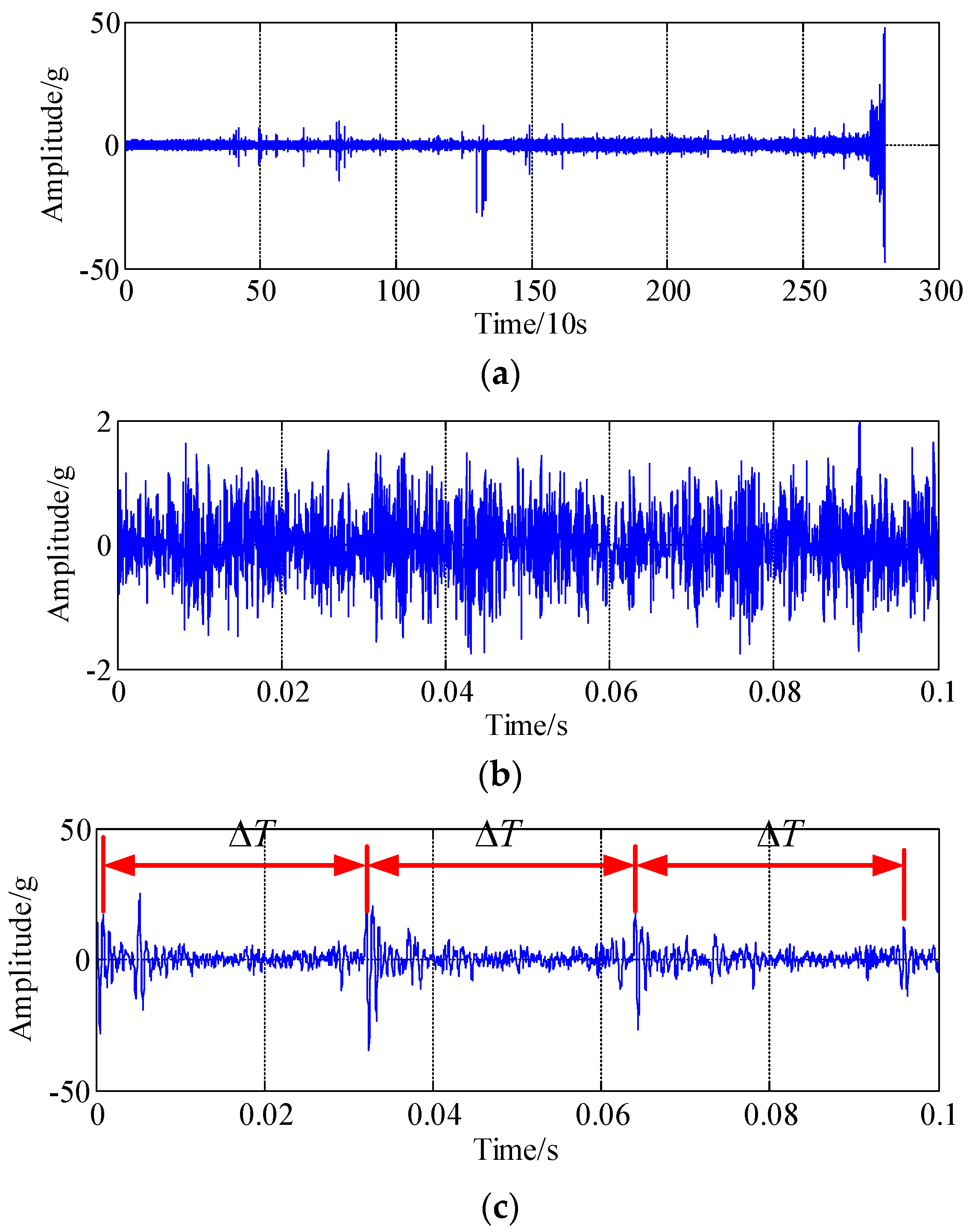
Figure 7a shows the whole lifetime data of a tested bearing in the time-domain, and the time-domain waveform of the tested bearing in the normal stage and the time-domain waveform of the tested bearing in the catastrophic failure stage are shown in Figure 7b,c, respectively. In the normal stage, the failure impulses cannot be observed in the time-domain, the range of the amplitude is [−2 g, 2 g]. However, in the failure stage, the range of the amplitude is [−50 g, 50 g], and there exist obvious impulses with time interval of , which is corresponding to the fault frequency of 169 Hz.
In this experiment, four bearings (bearing 1, bearing 2, bearing 3 and bearing 4) are randomly selected and employed as testing targets to evaluate the prediction performance. Each bearing is degraded during the accelerated life tests without implanting any artificial fault in advance.
- (1)
- bearing 1: operating conditions: speed 1800 rpm and load 4000 N; whole test life: 28,030 s;
- (1)
- bearing 2: operating conditions: speed 1800 rpm and load 4000 N; whole test life: 18,020 s;
- (1)
- bearing 3: operating conditions: speed 1650 rpm and load 4200 N; whole test life: 7970 s;
- (1)
- bearing 4: operating conditions: speed 1800 rpm and load 4000 N; whole test life: 14,280 s.
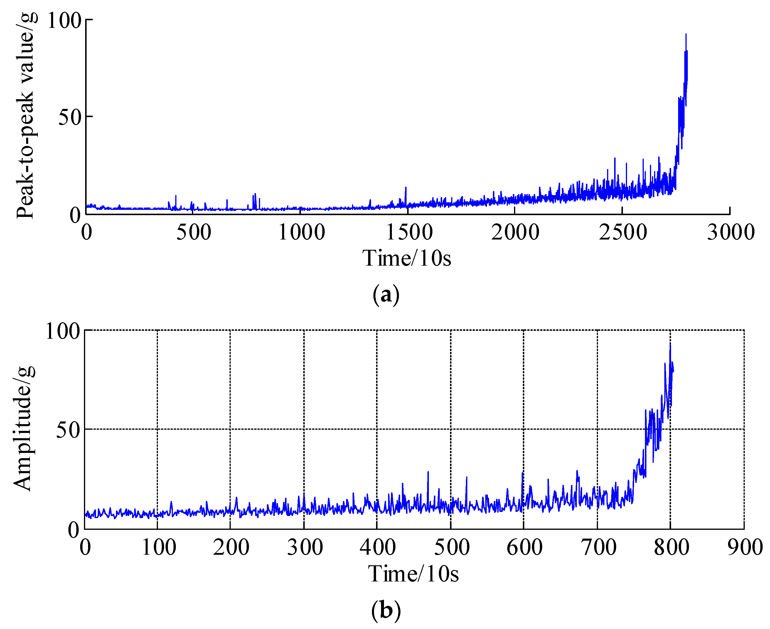
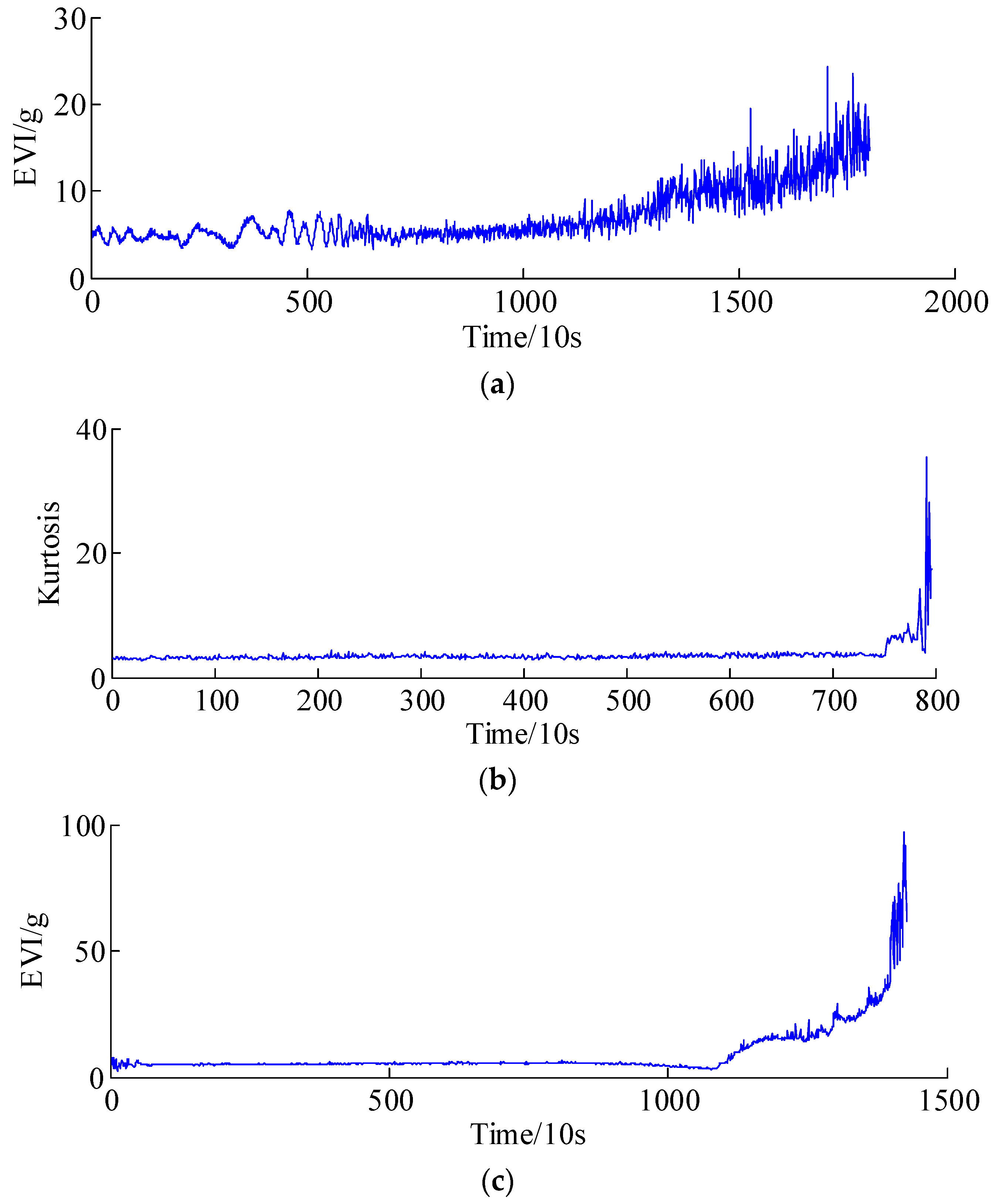
Depending on the diversity of operating conditions and the manufacturing accuracy of tested bearings, the effective running time may be different for different bearings. Therefore, the degradation trajectories of the health indicators are different for each tested bearing. Figure 8 shows the peak-to-peak values of the whole lifetime of bearing 1. Accordingly, the health indicators, i.e., equivalent vibration intensity (EVI) [9,11], Kurtosis and EVI of bearing 2, bearing 3 and bearing 4 are illustrated in Figure 9a–c, respectively. It is seen that the amplitudes of bearings 1, 3 and 4 have gradual increasing trends, in addition, the whole test life of bearing 3 is the shortest due to harsh operating conditions, which indicates that the extremely failures are occurred before the experiment stops, thus, representing abrupt degradation processes, whereas the EVI amplitudes of bearings 2 show gradual increases; it might be concluded that the design/manufacturing quality and fatigue resistance strength are much higher than others under the same operating conditions.
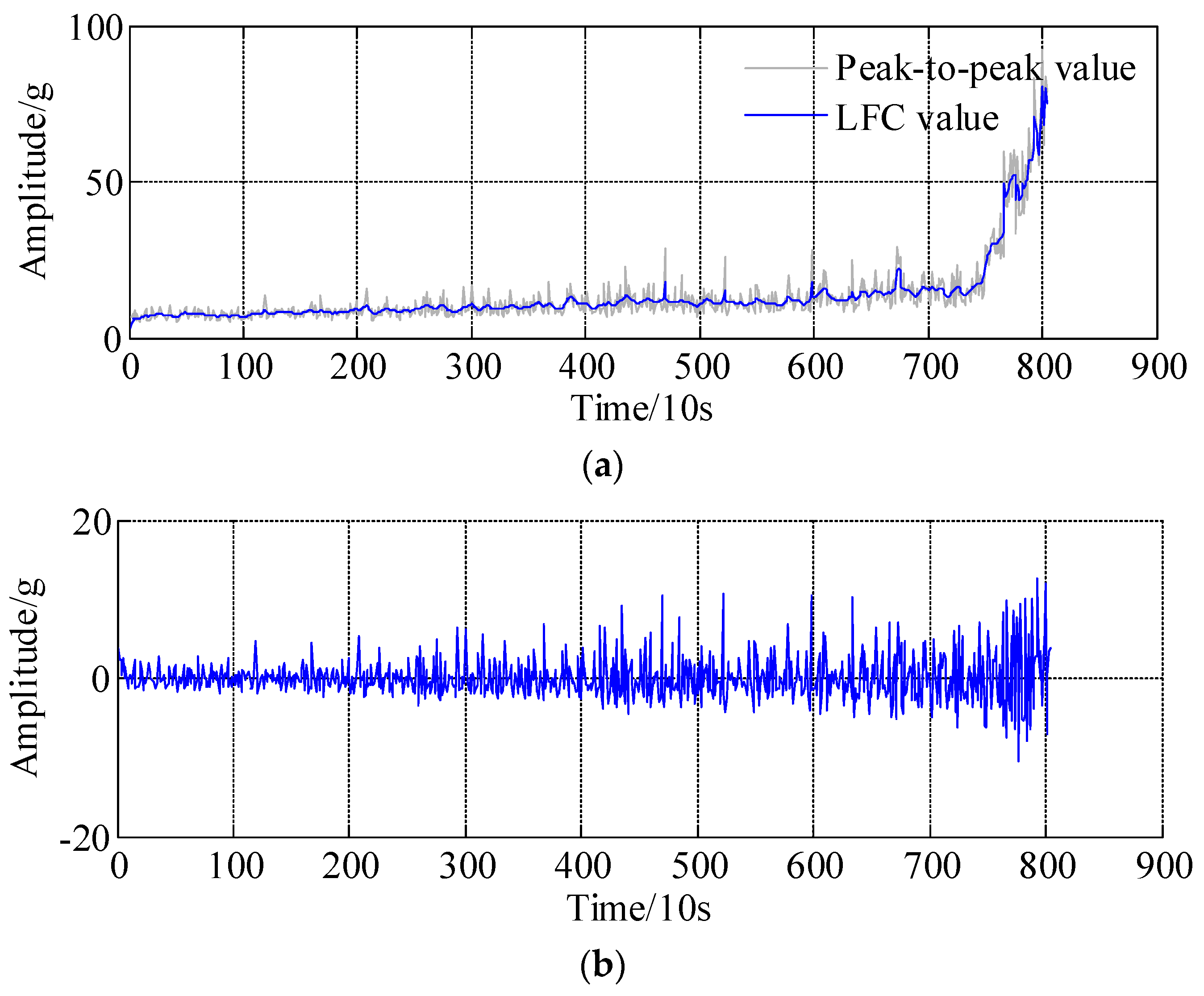
Taking bearing 1 as an example, as shown in Figure 8b, because of the abrupt degradation time series is the most interesting and difficult part; thus, datasets 2001 to 2803 are selected as survey regions, where the dataset from 2001 to 2703 are selected as a historical curve, and the remaining 100 datasets, i.e., dataset 2704 to dataset 2803, are a predicted region. Specifically, the proposed APSD method is adopted to process the peak-to-peak curve of bearing 1, since the standard deviation (SD) of the peak-to-peak is unknown, it can be calculated by the following equation, i.e., . Therefore, the related parameter specification of the APSD approach are summarized in Table 2. The decomposition results are presented in Figure 10, Figure 10a is the low frequency component and Figure 10b is the high frequency component, respectively. It should be noted that the low frequency component almost coincides with the actual peak-to-peak trends, especially in the abrupt degradation regions, which means the degradation processes and trend could be reflected by the low frequency component.
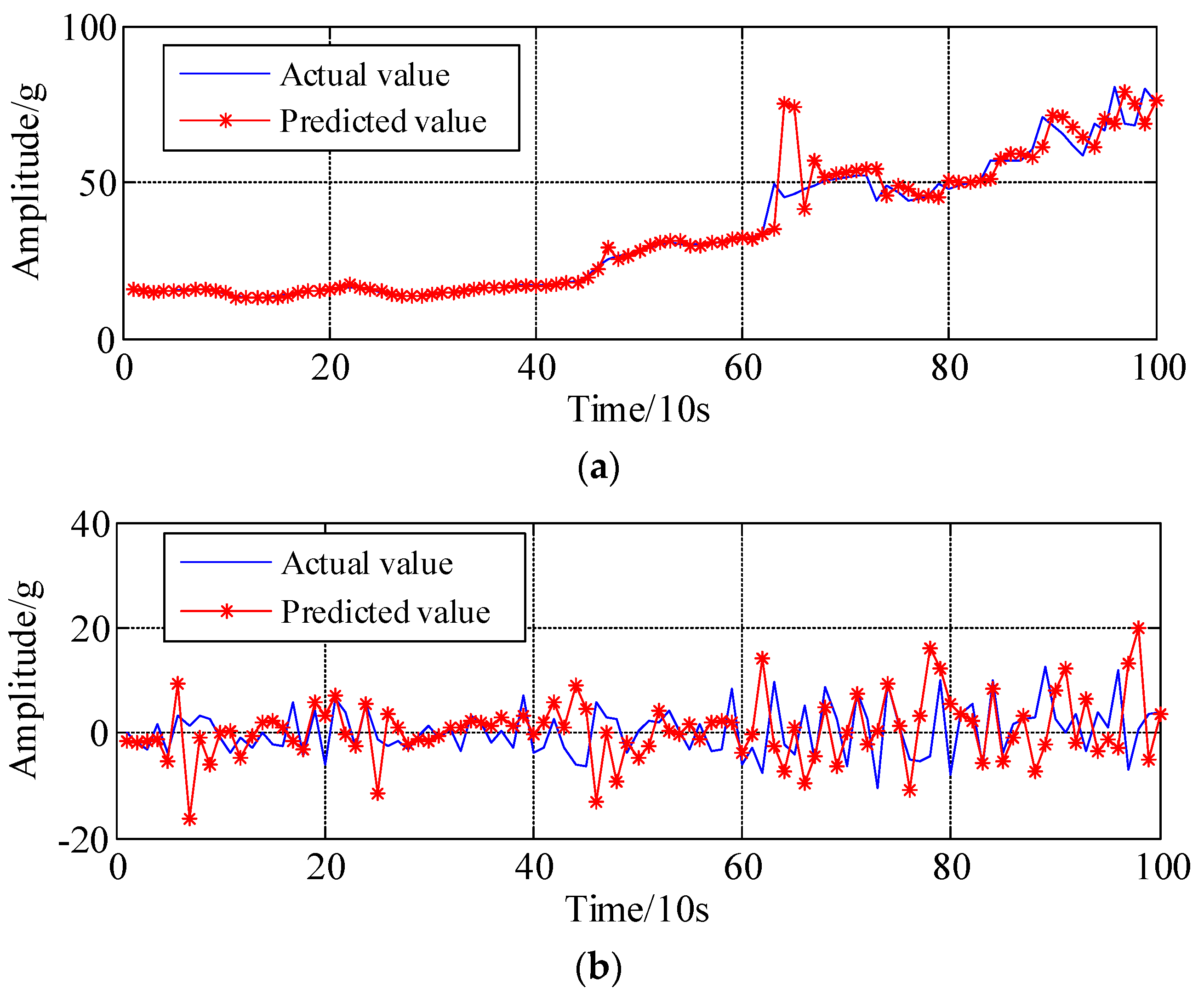
Furthermore, the WNN algorithm and ARMA-RLS model are introduced for prediction. For the prediction of a low frequency component, the number of input neurons, hidden neurons, output neurons, training iterations, learning rate for WNN are set at 7, 10, 1, 300 and 0.01, respectively. For the prediction of high frequency components, the modelling orders, i.e., p and q, are calculated by Akaike information criterion (AIC) criterion, and then all the parameters of ARMA are fed into the RLS learning algorithm; to recursively estimate and update the related parameters, the forgetting factor is set to 0.99. The prediction curves of the LFC and HFC for rolling bearing are illustrated in Figure 11a,b, respectively. As can be seen in Figure 11, the prediction data generated by the ANN and ARMA-RLS models are able to reasonably trace the variation trend of original peak-to-peak time series. The final predicted result can be correspondingly obtained by integrating the predicted LFC and HFC components, as shown in Figure 12.
As benchmarking approaches for the prognosis of bearing degradation trajectories, the ARMA, FARIMA and WNN, largest Lyapunov (LLyap) exponent models are employed for comparison. All the predicted results with the actual values are illustrated in Figure 12. As shown in Figure 12, all the benchmarking approaches could generally track the peak-to-peak fluctuation trend well except FARIMA because the memory function might be eliminated due to difference and inverse difference operating. Importantly, compared with the predicted results generated by benchmark approaches, the predictions created by the proposed method are closer to the actual values, and the specific quantitative comparison of the prediction performance are presented in following section.
Five assessment criteria of prediction results are introduced and calculated including mean absolute error (MAE), average relative error (ARE), root-mean-square error (RMSE), normalized mean square error (NMSE) and maximum of absolute error (Max-AE), which are denoted by,
where N is the number of time points, and are actual data and predicted data, respectively. Generally speaking, obviously, the smaller MAE, ARE, RMSE, NMSE and Max-AE values, which means lower prediction errors and higher prediction accuracies. The performance of the proposed methodology is evaluated by computed prediction errors. The computed prediction errors are summarized in Table 3. From the results in Table 3, it is noticed that the proposed method has relatively higher accuracy than FARIMA, WNN and L-Lyap methods. In addition, it is observed that the ARMA model has smaller errors among these models, but the tracking trend of LFC and fluctuation trend of HFC cannot be reflected at all; see black line in Figure 12. This indicates that the presented prediction approach has certain application potentials.
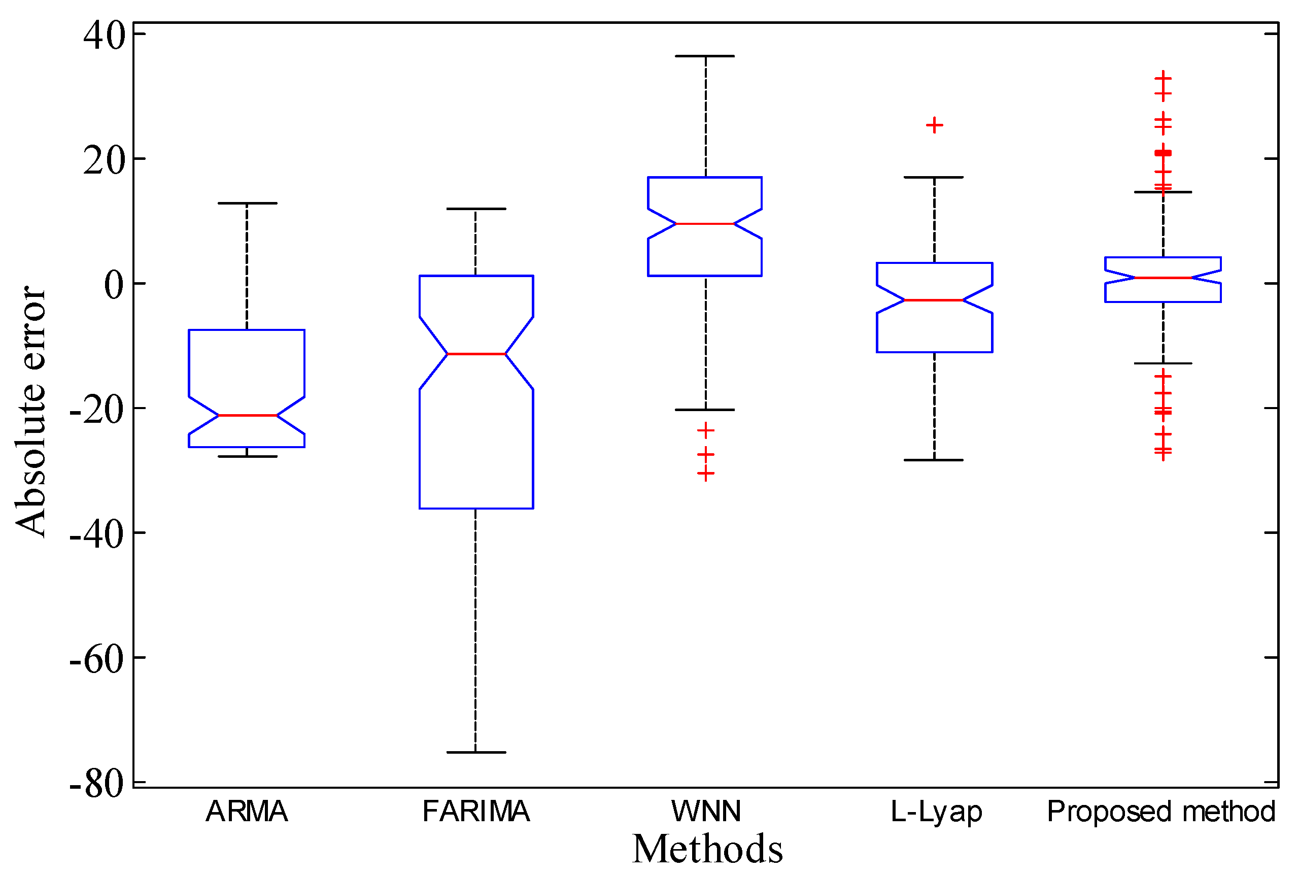
Meanwhile, to better evaluate the performances of all the methods from a statistical perspective, box plots were introduced. The box plots of all the errors based on benchmark approaches and proposed method are shown in Figure 13. The results show that the median values of the prediction errors converge to 0 based on proposed method, which demonstrate that the predicted data generated by the proposed approach are close to their true values.
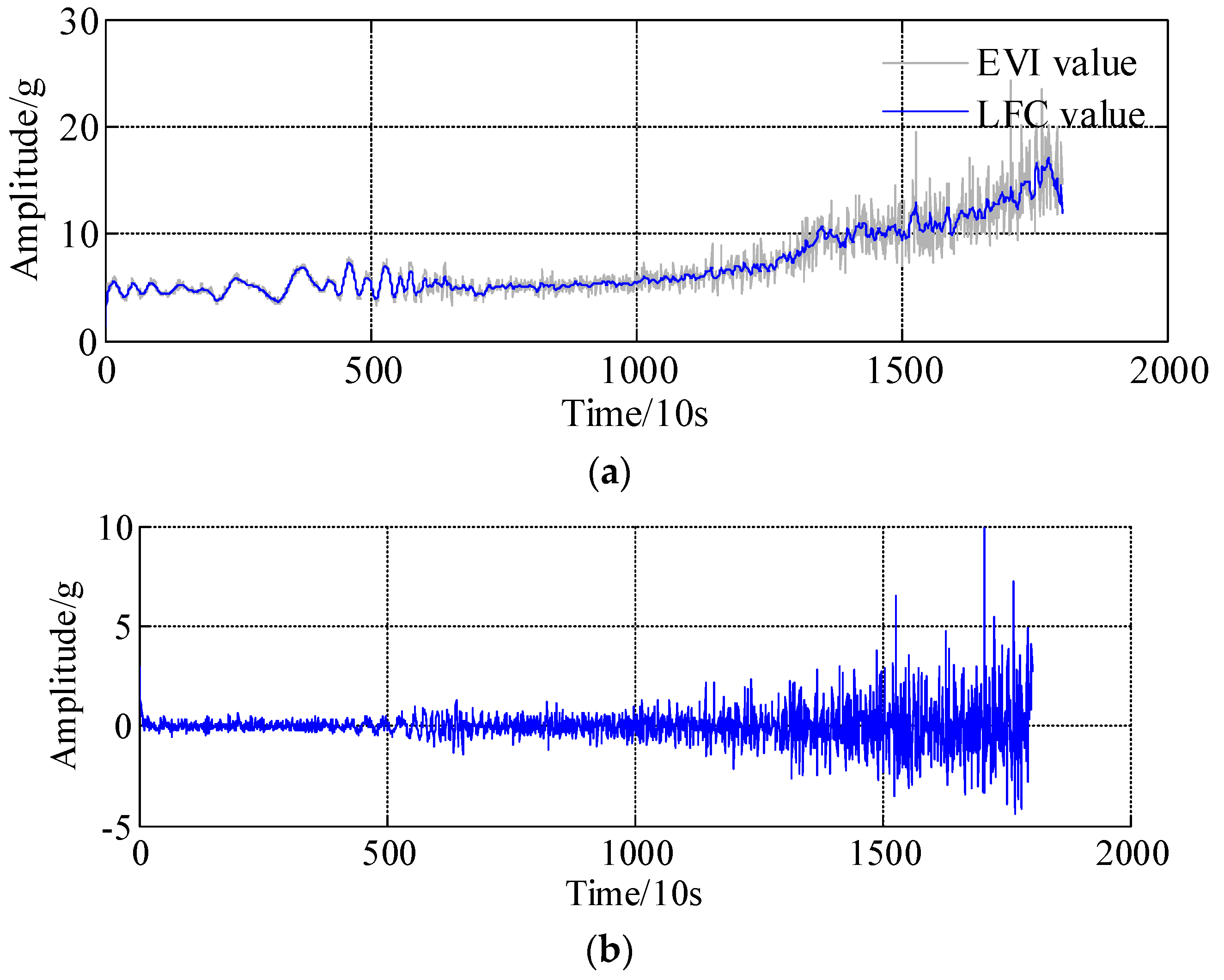
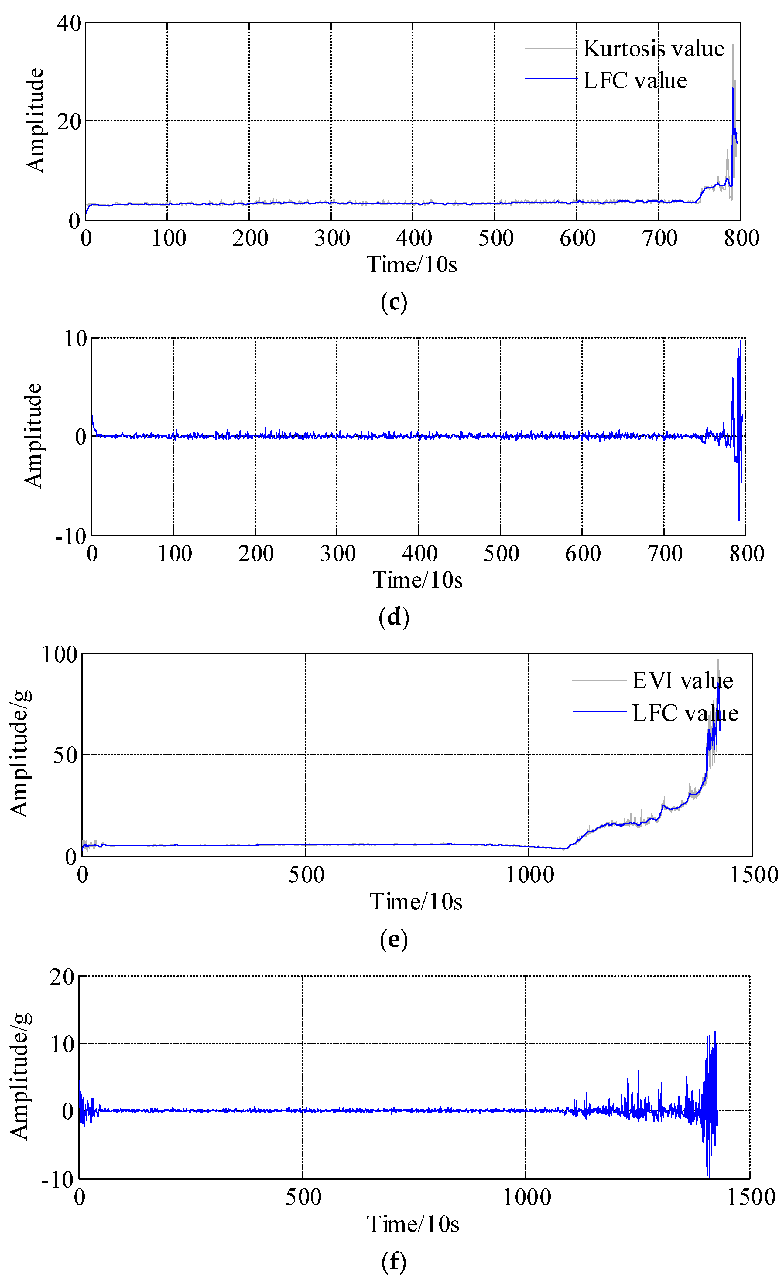
Furthermore, the prediction performances of the remaining bearings are illustrated in this section. The model parameter settings of the APSD, WNN, ARMA-RLS are similar to those in the aforementioned steps, the specific parameters are omitted here for the sake of simplification. The decomposition results, i.e., the LFC and HFC, of the bearing 2, bearing 3 and bearing 4 are respectively presented in Figure 14a–f; overall, it can be found that the low frequency component almost coincides with the actual health indicators trends, especially in the abrupt degradation regions.
The final predicted results of bearing 2, bearing 3 and bearing 4 are shown in Figure 15a–c, respectively. It is clear that all the predicted data converge to the actual data as time goes on. Interestingly, one can find that, the abrupt degradation points cannot be followed starting point, for example, the point 89 and point 90 in Figure 15b and point 72 in Figure 15c, nevertheless, subsequent points after those abrupt points could be restored, the reason is that the modeling parameters are updated by the artificial neural network and recursive least squares learning algorithm step by step, and the error is eliminated to the minimal range. The proposed two-step prediction method is more robust to the data collection errors. In conclusion, the proposed method performs best in the degradation trend prediction of the rolling bearings.
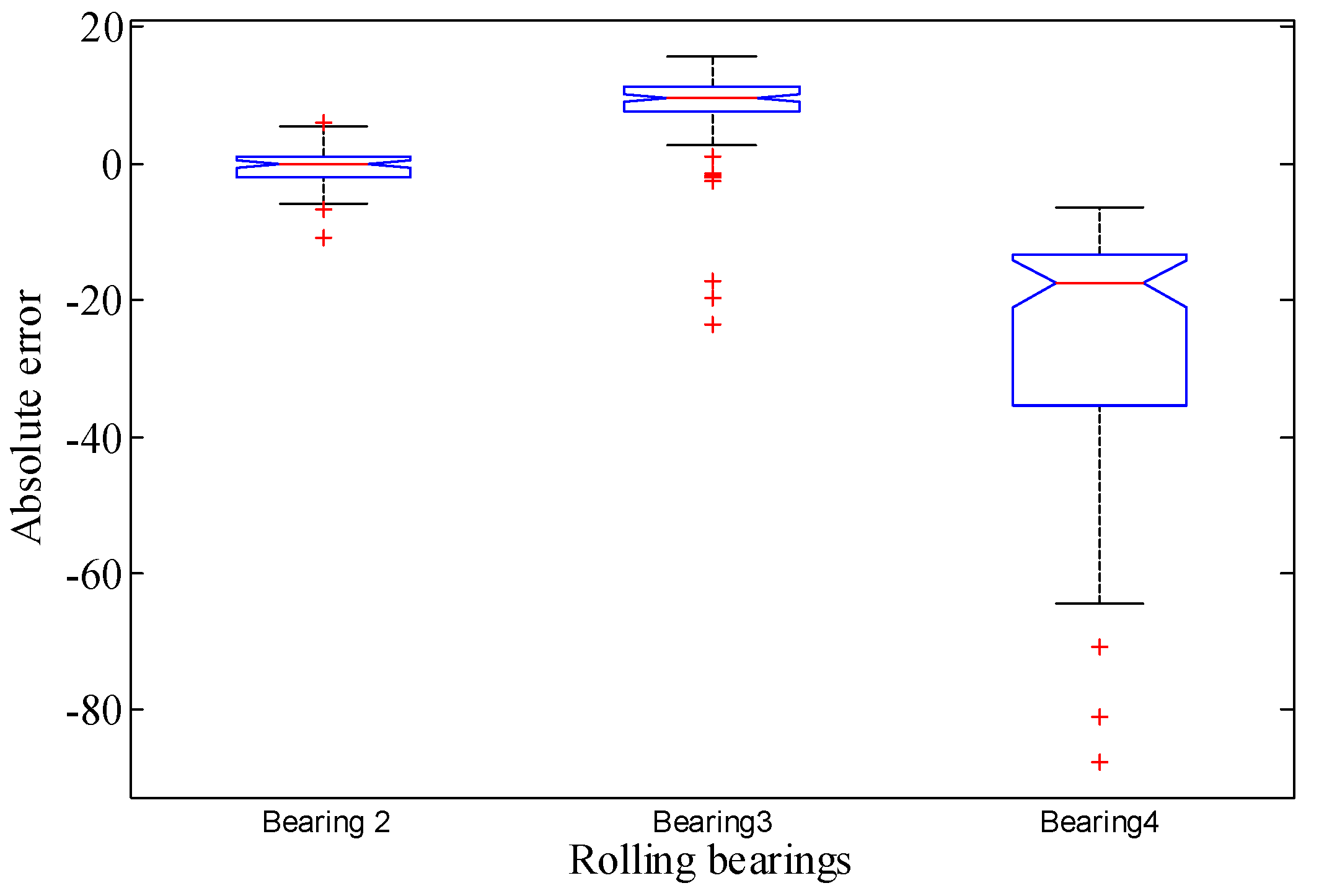
Additionally, Figure 16 summarizes the box plots of the absolute error (AE) of the remaining three bearings. Analogously, the box plots show that the median values of the absolute error of those three bearings converge to 0, which further reflects the effectiveness of the proposed method. Therefore, the proposed decomposition algorithm and prediction models have accurate prediction results.
5. Conclusions
Accurate prognosis of the degradation trend of rotating machinery plays an important role in industrial applications. Currently, most developments in the mechanical fault prognostics area have been targeted towards directly utilizing degradation-based data to trace the degradation trajectories, very few studies have used the idea of sparse decomposition. In this work, a novel intelligent prediction approach based on asymmetric penalty sparse decomposition (APSD) combined with WNN and ARMA-RLS models for health indicator degradation trajectories of four rolling bearings is proposed. The original health indicators od degradation trajectory are rearranged as two components, i.e., LFC and HFC. In particular, the HFC corresponds to the stable change around the zero line of health indicators, whereas the LFC is essentially related to the evolutionary trend of health indicators which rarely occurs in practice. The LFC and HFC are, respectively, predicted using the WNN and ARMA-RLS models. The final degradation regions (e.g., last 100 points) is correspondingly obtained by combining the predicted LFC and predicted HFC. Experimental results of four rolling bearings have demonstrated the superiority of the proposed method in terms of quantitative and qualitative evaluation compared to three commonly-used parametric-based and nonparametric-based methods, i.e., ARMA, FARIMA, WNN, L-Lyap methods.
This observation motivates the study of an integrated method for bearing prediction, which combines the strength of both parametric-based and nonparametric-based techniques. This paper focuses on the development of an intelligent degradation prognosis model that the error reverse transmission is employed to optimize the initial parameters of WNN, and the initial modelling parameters of ARMA are also optimized by the RLS algorithm step by step. The proposed method is more robust to different operating conditions and outperforms other one-step prediction methods by taking the LFC and HFC properties of health indicators into account. Therefore, the proposed method has huge potential in the field of PHM of mechanical equipment.
For future research, it would be interesting to investigate more advanced a sparse low-rank matrix decomposition (SLMD) algorithm to robustly separate the health indicator time series (HITS). Both LFC and HFC could be predicted using more sophisticated adaptive algorithms under more complex and harsh environments.
Author Contributions
Algorithms improvement, programming, experimental analysis and paper writing were done by Q.L. Review and suggestions were provided by S.Y.L. All authors have read and approved the final manuscript.
Acknowledgments
This research is supported the Fundamental Research Funds for the Central Universities (Grant Nos. CUSF-DH-D-2017059 and BCZD2018013) and the Research Funds of Worldtech Transmission Technology (Grant No. 12966EM).
Conflicts of Interest
The authors declare no conflict of interest.
References
- Chen, Z.Y.; Li, W.H. Multisensor feature fusion for bearing fault diagnosis using sparse autoencoder and deep belief network. IEEE Trans. Instrum. Meas. 2017, 66, 1693–1702. [Google Scholar] [CrossRef]
- Singleton, R.K.; Strangas, E.G.; Aviyente, S. The use of bearing currents and vibrations in lifetime estimation of bearings. IEEE Trans. Ind. Inform. 2017, 13, 1301–1309. [Google Scholar] [CrossRef]
- Li, Q.; Ji, X.; Liang, S.Y. Incipient fault feature extraction for rotating machinery based on improved AR-minimum entropy deconvolution combined with variational mode decomposition approach. Entropy 2017, 19, 317. [Google Scholar] [CrossRef]
- Lei, Y.G.; Li, N.P.; Guo, L.; Li, N.B.; Yan, T.; Lin, J. Machinery health prognostics: A systematic review from data acquisition to RUL prediction. Mech. Syst. Signal Process. 2018, 104, 799–834. [Google Scholar] [CrossRef]
- Li, Q.; Liang, S.Y.; Song, W.Q. Revision of bearing fault characteristic spectrum using LMD and interpolation correction algorithm. Procedia CIRP 2016, 56, 182–187. [Google Scholar] [CrossRef]
- Li, Q.; Hu, W.; Peng, E.F.; Liang, S.Y. Multichannel signals reconstruction based on tunable Q-factor wavelet transform-morphological component analysis and sparse Bayesian iteration for rotating machines. Entropy 2018, 20, 263. [Google Scholar] [CrossRef]
- Hong, S.; Zhou, Z.; Zio, E.; Wang, W.B. An adaptive method for health trend prediction of rotating bearings. Digit. Signal Process. 2014, 35, 17–123. [Google Scholar] [CrossRef]
- Rojas, I.; Valenzuela, O.; Rojasa, F.; Guillen, A.; Herrera, L.J.; Pomares, H.; Marquez, L.; Pasadas, M. Soft-computing techniques and ARMA model for time series prediction. Neurocomputing 2008, 71, 519–537. [Google Scholar] [CrossRef]
- Li, Q.; Liang, S.Y.; Yang, J.G.; Li, B.Z. Long range dependence prognostics for bearing vibration intensity chaotic time series. Entropy 2016, 18, 23. [Google Scholar] [CrossRef]
- Li, M.; Zhang, P.D.; Leng, J.X. Improving autocorrelation regression for the Hurst parameter estimation of long-range dependent time series based on golden section search. Phys. A 2016, 445C, 189–199. [Google Scholar] [CrossRef]
- Li, Q.; Liang, S.Y. Degradation trend prognostics for rolling bearing using improved R/S statistic model and fractional Brownian motion approach. IEEE Access 2018, 6, 21103–21114. [Google Scholar] [CrossRef]
- Song, W.; Li, M.; Liang, J.K. Prediction of bearing fault using fractional brownian motion and minimum entropy deconvolution. Entropy 2016, 18, 418. [Google Scholar] [CrossRef]
- Peng, Y.; Dong, M. A prognosis method using age-dependent hidden semi-Markov model for equipment health prediction. Mech. Syst. Signal Process. 2011, 25, 237–252. [Google Scholar] [CrossRef]
- Yan, J.H.; Guo, C.Z.; Wang, X. A dynamic multi-scale Markov model based methodology for remaining life prediction. Mech. Syst. Signal Process. 2011, 25, 1364–1376. [Google Scholar] [CrossRef]
- Tien, T.L. A research on the prediction of machining accuracy by the deterministic grey dynamic model DGDM (1,1,1). Appl. Math. Comput. 2005, 161, 923–945. [Google Scholar] [CrossRef]
- Abdulshahed, A.M.; Longstaff, A.P.; Fletcher, S.; Potdar, A. Thermal error modelling of a gantry-type 5-axis machine tool using a grey neural network model. J. Manuf. Syst. 2016, 41, 130–142. [Google Scholar] [CrossRef]
- Santhosh, T.V.; Gopika, V.; Ghosh, A.K.; Fernandes, B.G. An approach for reliability prediction of instrumentation & control cables by artificial neural networks and Weibull theory for probabilistic safety assessment of NPPs. Reliab. Eng. Syst. Saf. 2018, 170, 31–44. [Google Scholar]
- Torkashvand, A.M.; Ahmadi, A.; Nikravesh, N.L. Prediction of kiwifruit firmness using fruit mineral nutrient concentration by artificial neural network (ANN) and multiple linear regressions (MLR). J. Integr. Agric. 2017, 16, 1634–1644. [Google Scholar] [CrossRef]
- Lazakis, I.; Raptodimos, Y.; Varelas, T. Predicting ship machinery system condition through analytical reliability tools and artificial neural networks. Ocean Eng. 2018, 152, 404–415. [Google Scholar] [CrossRef]
- Dhamande, L.S.; Chaudhari, M.B. Detection of combined gear-bearing fault in single stage spur gear box using artificial neural network. Procedia Eng. 2016, 144, 759–766. [Google Scholar] [CrossRef]
- Chen, C.C.; Vachtsevanos, G. Bearing condition prediction considering uncertainty: An interval type-2 fuzzy neural network approach. Robot. Comput. Int. Manuf. 2012, 28, 509–516. [Google Scholar] [CrossRef]
- Ren, L.; Cui, J.; Sun, Y.Q.; Cheng, X.J. Multi-bearing remaining useful life collaborative prediction: A deep learning approach. J. Manuf. Syst. 2017, 43, 248–256. [Google Scholar] [CrossRef]
- Deutsch, J.; He, D. Using deep learning-based approach to predict remaining useful life of rotating components. IEEE Trans. Syst. Man Cybern. Syst. 2018, 48, 11–20. [Google Scholar] [CrossRef]
- Selesnick, I.W.; Bayram, I. Enhanced sparsity by non-separable regularization. IEEE Trans. Signal Process. 2016, 64, 2298–2313. [Google Scholar] [CrossRef]
- He, W.P.; Ding, Y.; Zi, Y.Y.; Selesnick, I.W. Repetitive transients extraction algorithm for detecting bearing faults. Mech. Syst. Signal Process. 2017, 84, 227–244. [Google Scholar] [CrossRef] [Green Version]
- Li, Q.; Liang, S.Y. Multiple faults detection for rotating machinery based on Bi-component sparse low-rank matrix separation approach. IEEE Access 2018, 6, 20242–20254. [Google Scholar] [CrossRef]
- Li, Q.; Liang, S.Y. Bearing incipient fault diagnosis based upon maximal spectral kurtosis TQWT and group sparsity total variation de-noising approach. J. Vibroeng. 2018, 20, 1409–1425. [Google Scholar] [CrossRef]
- Wang, S.B.; Selesnick, I.W.; Cai, G.G.; Feng, Y.N.; Sui, X.; Chen, X.F. Nonconvex sparse regularization and convex optimization for bearing fault diagnosis. IEEE Trans. Ind. Electron. 2018, 65, 7332–7342. [Google Scholar] [CrossRef]
- Parekh, A.; Selesnick, I.W. Enhanced low-rank matrix approximation. IEEE Signal Process. Lett. 2016, 23, 493–497. [Google Scholar] [CrossRef]
- Parekh, A.; Selesnick, I.W. Convex fused lasso denoising with non-convex regularization and its use for pulse detection. In Proceedings of the IEEE Signal Processing in Medicine and Biology Symposium, Philadelphia, PA, USA, 12 December 2015; pp. 1–6. [Google Scholar]
- Ding, Y.; He, W.P.; Chen, B.Q.; Zi, Y.Y.; Selesnick, I.W. Detection of faults in rotating machinery using periodic time-frequency sparsity. J. Sound Vib. 2016, 382, 357–378. [Google Scholar] [CrossRef] [Green Version]
- Donoho, D.L. Compressed sensing. IEEE Trans. Inf. Theory 2006, 52, 1289–1306. [Google Scholar] [CrossRef]
- Donoho, D.L.; Tsaig, Y. Fast solution of ℓ1-norm minimization problems when the solution may be sparse. IEEE Trans. Inf. Theory 2008, 54, 4789–4812. [Google Scholar] [CrossRef]
- Donoho, D.L. De-noising by soft-thresholding. IEEE Trans. Inf. Theory 1995, 41, 613–627. [Google Scholar] [CrossRef] [Green Version]
- Selesnick, I.W. Total variation denoising via the Moreau envelope. IEEE Signal Process. Lett. 2017, 24, 216–220. [Google Scholar] [CrossRef]
- Selesnick, I.W.; Parekh, A.; Bayram, I. Convex 1-D total variation denoising with non-convex regularization. IEEE Signal Process. Lett. 2015, 22, 141–144. [Google Scholar] [CrossRef]
- Selesnick, I.W.; Graber, H.L.; Pfeil, D.S.; Barbour, R.L. Simultaneous low-pass filtering and total variation denoising. IEEE Trans. Signal Process. 2014, 62, 1109–1124. [Google Scholar] [CrossRef]
- Ning, X.R.; Selesnick, I.W.; Duval, L. Chromatogram baseline estimation and denoising using sparsity (BEADS). Chemom. Intell. Lab. Syst. 2014, 139, 156–167. [Google Scholar] [CrossRef]
- Mourad, N.; Reilly, J.P.; Kirubarajan, T. Majorization-minimization for blind source separation of sparse sources. Signal Process. 2017, 131, 120–133. [Google Scholar] [CrossRef]
- Hunter, D.R.; Lange, K. Quantile Regression via an MM Algorithm. J. Comput. Graph. Stat. 2000, 9, 60–77. [Google Scholar] [Green Version]
- Donoho, D.; Johnstone, I.; Johnstone, I.M. Ideal spatial adaptation by wavelet shrinkage. Biometrika 1993, 81, 425–455. [Google Scholar] [CrossRef]
- Singh, K.R.; Chaudhury, S. Efficient technique for rice grain classification using back-propagation neural network and wavelet decomposition. IET Comput. Vis. 2016, 10, 780–787. [Google Scholar] [CrossRef]
- Heermann, P.D.; Khazenie, N. Classification of multispectral remote sensing data using a back-propagation neural network. IEEE Trans. Geosci. Remote 1992, 30, 81–88. [Google Scholar] [CrossRef]
- Chen, F.C. Back-propagation neural networks for nonlinear self-tuning adaptive control. IEEE Control. Syst. Mag. 1990, 10, 44–48. [Google Scholar] [CrossRef] [Green Version]
- Zeng, Y.R.; Zeng, Y.; Choi, B.; Wang, L. Multifactor-influenced energy consumption forecasting using enhanced back-propagation neural network. Energy 2017, 127, 381–396. [Google Scholar] [CrossRef]
- Osofsky, S.S. Calculation of transient sinusoidal signal amplitudes using the Morlet wavelet. IEEE Trans. Signal Process. 1999, 47, 3426–3428. [Google Scholar] [CrossRef]
- Büssow, R. An algorithm for the continuous Morlet wavelet transform. Mech. Syst. Signal Process. 2007, 21, 2970–2979. [Google Scholar] [CrossRef] [Green Version]
- Ji, W.; Chee, K.C. Prediction of hourly solar radiation using a novel hybrid model of ARMA and TDNN. Sol. Energy 2011, 85, 808–817. [Google Scholar] [CrossRef]
- Brockwell, P.J.; Davis, R.A. Time Series: Theory and Methods, 2nd ed.; Springer: New York, NY, USA, 2009; ISBN 9781441903198. [Google Scholar]
- Ogasawara, H. Bias correction of the Akaike information criterion in factor analysis. J. Multivar. Anal. 2016, 149, 144–159. [Google Scholar] [CrossRef]
- Nectoux, P.; Gouriveau, R.; Medjaher, K.; Ramasso, E.; Morello, B.; Zerhouni, N.; Varnier, C. Pronostia: An experimental platform for bearings accelerated life test. In Proceedings of the IEEE International Conference on Prognostics and Health Management, Denver, CO, USA, 12 June 2012. [Google Scholar]
- Benkedjouh, T.; Medjaher, K.; Zerhouni, N.; Rechak, S. Remaining useful life estimation based on nonlinear feature reduction and support vector regression. Eng. Appl. Artif. Intell. 2013, 26, 1751–1760. [Google Scholar] [CrossRef]
Figure 1.
Typical bearing degradation trajectories described by the bearing health indicators.

Figure 2.
The plot of the asymmetric penalty function

Figure 3.
The decomposition results of noisy chromatogram data using proposed APSD algorithm [38]. (a) The raw data with additive noise; (b) The estimated LFC signal; (c) The estimated HFC signal.
Figure 3.
The decomposition results of noisy chromatogram data using proposed APSD algorithm [38]. (a) The raw data with additive noise; (b) The estimated LFC signal; (c) The estimated HFC signal.

Figure 4.
The structural diagram of wavelet neural network.

Figure 5.
Flow chart of wavelet neural network (WNN) for prediction of low frequency data.

Figure 6.
Experimental setup. (a) Overview of experimental setup; (b) Normal and degraded bearings [51,52].

Figure 7.
Raw signal of a tested bearing. (a) The historical signals of the whole lifetime; (b) The time-domain waveform of the bearing in the normal stage; (c) The time-domain waveform of the bearing in the failure stage.
Figure 7.
Raw signal of a tested bearing. (a) The historical signals of the whole lifetime; (b) The time-domain waveform of the bearing in the normal stage; (c) The time-domain waveform of the bearing in the failure stage.

Figure 8.
The health indicator curve of peak-to-peak value of bearing 1. (a) The peak-to-peak value of the whole lifetime of bearing 1; (b) The peak-to-peak value of the point 2001 from to point 2803.
Figure 8.
The health indicator curve of peak-to-peak value of bearing 1. (a) The peak-to-peak value of the whole lifetime of bearing 1; (b) The peak-to-peak value of the point 2001 from to point 2803.

Figure 9.
The health indicator curves of different bearings. (a) The equivalent vibration intensity curve of bearing 2; (b) The Kurtosis curve of bearing 3; (c) The equivalent vibration intensity curve of bearing 4.
Figure 9.
The health indicator curves of different bearings. (a) The equivalent vibration intensity curve of bearing 2; (b) The Kurtosis curve of bearing 3; (c) The equivalent vibration intensity curve of bearing 4.

Figure 10.
Decomposition results of low frequency component (LFC) and high frequency component (HFC) based on asymmetric penalty sparse decomposition. (a) The low frequency component (LFC); (b) The high frequency component (HFC).
Figure 10.
Decomposition results of low frequency component (LFC) and high frequency component (HFC) based on asymmetric penalty sparse decomposition. (a) The low frequency component (LFC); (b) The high frequency component (HFC).

Figure 11.
Prediction results of LFC and HFC based on WNN and ARMA-RLS method, respectively. (a) Predicted result of LFC based on WNN method; (b) Predicted results of HFC based on ARMA-RLS method.
Figure 11.
Prediction results of LFC and HFC based on WNN and ARMA-RLS method, respectively. (a) Predicted result of LFC based on WNN method; (b) Predicted results of HFC based on ARMA-RLS method.

Figure 12.
Comparison of the forecasting for peak-to-peak series using benchmarking methods and proposed approach.
Figure 12.
Comparison of the forecasting for peak-to-peak series using benchmarking methods and proposed approach.

Figure 13.
Quantitative performance evaluation based on absolute error boxplot.

Figure 14.
Decomposition results of LFC and HFC based on asymmetric penalty sparse decomposition. (a) The low frequency component of bearing 2; (b) The High frequency component of bearing 2; (c) The low frequency component of bearing 3; (d) The High frequency component of bearing 3; (e) The low frequency component of bearing 4; (f) The High frequency component of bearing 4.


Figure 15.
The predicted results of remaining three bearings. (a) The predicted results of bearing 2; (b) the predicted results of bearing 3; (c) the predicted results of bearing 4.
Figure 15.
The predicted results of remaining three bearings. (a) The predicted results of bearing 2; (b) the predicted results of bearing 3; (c) the predicted results of bearing 4.

Figure 16.
Quantitative performance evaluation based on absolute error boxplot of remaining three bearings.
Figure 16.
Quantitative performance evaluation based on absolute error boxplot of remaining three bearings.


Table 1.
Symmetric penalty functions and their derivatives.
| Functions | ||
|---|---|---|
Table 2.
The parameters setting of APSD method for bearing 1.
| Parameters β0 | Parameters γ | Regularization Parameter λ0 | Regularization Parameter λ1 | Regularization Parameter λ2 | M-Term | Iteration Times |
|---|---|---|---|---|---|---|
| β0 = 0.8 | γ = 7.5 | λ0 = 1.7400 | λ1 = 3.2625 | λ2 = 1.7400 | 2 | 50 |
Table 3.
The computed prediction errors of proposed method and benchmark methods.
| Index | ARMA | FARIMA | WNN | L-Lyap | Proposed |
|---|---|---|---|---|---|
| Mean Absolute Error-MAE | 0.5880 | 17.2700 | 8.2364 | 3.2453 | 0.9770 |
| Average relative error-ARE | 0.1872 | 0.4666 | 0.1583 | 0.2691 | 0.2599 |
| Root-Mean-Square Error-RMSE | 5.9094 | 173.5702 | 82.7793 | 32.6164 | 9.8190 |
| Normalized Mean Square Error-NMSE | 0.1657 | 2.4144 | 0.7173 | 0.3008 | 0.2244 |
| Maximum of Absolute Error-MaxAE | 21.9865 | 75.0981 | 36.4112 | 28.3548 | 32.9561 |
© 2018 by the authors. Licensee MDPI, Basel, Switzerland. This article is an open access article distributed under the terms and conditions of the Creative Commons Attribution (CC BY) license (http://creativecommons.org/licenses/by/4.0/).
Share and Cite
MDPI and ACS Style
Li, Q.; Liang, S.Y. Intelligent Prognostics of Degradation Trajectories for Rotating Machinery Based on Asymmetric Penalty Sparse Decomposition Model. Symmetry 2018, 10, 214. https://doi.org/10.3390/sym10060214
AMA Style
Li Q, Liang SY. Intelligent Prognostics of Degradation Trajectories for Rotating Machinery Based on Asymmetric Penalty Sparse Decomposition Model. Symmetry. 2018; 10(6):214. https://doi.org/10.3390/sym10060214
Chicago/Turabian StyleLi, Qing, and Steven Y. Liang. 2018. "Intelligent Prognostics of Degradation Trajectories for Rotating Machinery Based on Asymmetric Penalty Sparse Decomposition Model" Symmetry 10, no. 6: 214. https://doi.org/10.3390/sym10060214
Note that from the first issue of 2016, this journal uses article numbers instead of page numbers. See further details here.