A Hybrid Fuzzy Analytic Network Process (FANP) and Data Envelopment Analysis (DEA) Approach for Supplier Evaluation and Selection in the Rice Supply Chain

Abstract

In the market economy, competition is typically due to the difficulty in selecting the most suitable supplier, one that is capable to help a business to develop a profit to the highest value threshold and capable to meet sustainable development features. In addition, this research discusses a wide range of consequences from choosing an effective supplier, including reducing production cost, improving product quality, delivering the product on time, and responding flexibly to customer requirements. Therefore, the activities noted above are able to increase an enterprise’s competitiveness. It can be seen that selecting a supplier is complex in that decision-makers must have an understanding of the qualitative and quantitative features for assessing the symmetrical impact of the criteria to reach the most accurate result. In this research, the multi-criteria group decision-making (MCGDM) approach was proposed to solve supplier selection problems. The authors collected data from 25 potential suppliers, and the four main criteria within contain 15 sub-criteria to define the most effective supplier, which has viewed factors, including financial efficiency guarantee, quality of materials, ability to deliver on time, and the conditioned response to the environment to improve the efficiency of the industry supply chain. Initially, fuzzy analytic network process (ANP) is used to evaluate and rank these criteria, which are able to be utilized to clarify important criteria that directly affect the profitability of the business. Subsequently, data envelopment analysis (DEA) models, including the Charnes Cooper Rhodes model (CCR model), Banker Charnes Cooper model (BCC model), and slacks-based measure model (SBM model), were proposed to rank suppliers. The result of the model has proposed 7/25 suppliers, which have a condition response to the enterprises’ supply requirements.

1. Introduction

The task of selecting suppliers becomes more important in today’s competitive and global environment when it is impractical or virtually impossible to create high-quality, low-cost, successful products without a vendor. For businesses today, vendor selection is one of the most important and indispensable components of the supply chain function of Florez–Lopez [1]. The enterprises’ expected goal of selecting a vendor is necessary to reduce the risk in buying, making an optimum decision, and establishing a sustainable alliance between buyers and suppliers [2]. Basically, choosing suppliers is a decision-making process because a business expects to obtain a supplier [3]. Additionally, it requires a powerful analytical approach, via utilizing decision-support tools, which is capable of addressing multiple criteria [4]. Incidentally, the supplier’s price includes many qualitative and qualitative conflicts.

The author represents two techniques, i.e., DEA and the FANP, which are used to design a method for evaluating suppliers. In order to obtain the accurate result as the chosen supplier based on the frontier point of the DEA model from input and output decision-makers (DMUs) [5]. The drawback of DEA, related to this study, is the requirement of data for various inputs and outputs to be in a quantitative format. This DEA limitation is addressed by analyzing the qualitative factors/attributes associated with the supplier using FANP. FANP is a more general form of the decentralized process, which includes the feedback and interdependencies of decision attributes and alternatives. This additional feature provides a more accurate and robust approach when modeling a complex decision-making environment [6].

The decision-making process is designed to provide a holistic approach in which the relevant factors and criteria are integrated into the FANP’s decentralized network. Different relationships are combined in these structures and then both judgment and logic are used to estimate the relative effect from which the overall response is derived [7]. The FANP model used here provides a unique quantitative value for vendor-specific qualitative factors and is based on buyers’ preferences and perceptions. This quantitative value from FANP for each supplier is used as a qualitative benefit in the DEA model to obtain the ranking or performance of different suppliers.

This research proposed hybrid FANP and DEA approaches for supplier selection in the rice supply chain, which also considers green issues under uncertain environment conditions. The aim of this research is to provide a useful guideline for supplier selection based on qualitative and quantitative factors (including the main criteria, such as financial, delivery services, qualitative factors, and environmental management systems) to improve the efficiency of supplier selection in the rice supply chain and other industries.

In the remainder of this paper, this research provides the platform data to further support the need of the development of a decision approach. Then, the synthetic supplier evaluation approach was applied to a case study of a company, which could be used for the explanation of the findings. Finally, this paper ends with a summary, and conclusions are made.

2. Literature Review

2.1. Supplier Selection Methods

Aissaoui et al. [8] presented a literature review that covers the entire purchasing process, considered both parts and services outsourcing activities, and covers Internet-based procurement environments, such as electronic marketplace auctions. Govindan et al. [9] presented a literature review for multi-criteria decision-making approaches for green supplier evaluation and selection. Chai et al. [10] provided a systematic literature review on articles published from 2008 to 2012 on the application of DM techniques for supplier selection.

Wu and Blackhurst [11] proposed a methodology termed augmented DEA, which has enhanced discriminatory power over basic DEA models to rank suppliers. Amirteimoori and Khoshandam [12] developed a DEA model for evaluating the performance of suppliers and manufacturers in supply chain operations. Lin et al. [13] provided a MCDM model by combining the Delphi method and the ANP method for evaluating and selecting suppliers for the sustainable operation and development of enterprises in the aerospace industry. Galankashi et al. [14] proposed an integrated balanced scorecard (BSC) and fuzzy analytic hierarchical process (FAHP) model to select suppliers in the automotive industry. Kilincci and Onal [15] used a fuzzy AHP approach for supplier selection in a washing machine company.

Tyagi et al. [16] proposed fuzzy AHP and AHP methods to prioritize the alternatives of the supply chain performance system. Karsak and Dursun [17] proposed a fuzzy MCDM model including the quality function deployment (QFD), fusion of fuzzy information, and 2-tuple linguistic representation for supplier evaluation and selection. Chen et al. [18] proposed a hybrid AHP and TOPSIS for evaluating and ranking the potential suppliers. Guo et al. [19] used fuzzy MCDM approaches for green supplier selection in apparel manufacturing. Wu et al. [20] constructed a multiple criteria decision-making model for the selection of fishmeal suppliers. Hu et al. [21] proposed a hybrid fuzzy DEA/AHP methodology for ranking units in a fuzzy environment. He and Zhang [22] used a hybrid evaluation model based on factor analysis (FA), data envelopment analysis (DEA), with analytic hierarchy process (AHP) for a supplier selection from the perspective of a low-carbon supply chain.

Parkouhi et al. [23] used the fuzzy analytic network process and VlseKriterijuska Optimizacija I Komoromisno Resenje (VIKOR) techniques for supplier selection. Wan et al. [24] proposed a hybrid DEA and Grey Model (1,1) approach for partner selection in the supply chain of Vietnam’s textile and apparel industry. Wu et al. [25] used the fuzzy Delphi method, ANP, and TOPSIS for supplier selection. Rezaeisaray et al. [26] proposed a hybrid DEMATLE, FANP, and DEA model for outsourcing supplier selection in pipe and fittings manufacturing. Rouyendegh and Erol [27] applied the DEA-fuzzy ANP for department ranking at Iran Amirkabir University. Fuzzy set theory formalized by Zadeh [28] is an effective tool, which has been widely used in the supplier selection decision process because it provides a suitable language to transform imprecise criteria to precise criteria.

Junior et al. [29] presented a comparison between fuzzy AHP and fuzzy TOPSIS methods to supplier selection. The linear programming of data envelopment analysis (DEA), which is proposed by Charnes et al. [30], and is able to produce the result of measured efficiency without having specific weights for inputs and outputs or specify the form of the production function, is a nonparametric technique used to measure the relative efficiency of peer decision-making units with multiple inputs and outputs [31,32]. In the supplier’s evaluation and selection process, many researchers calculated the supplier’s performance by using the ratio of weighted outputs to weighted inputs [32]. Thus, the integrated FANP and DEA method is used to determine supplier selection criteria and select supplier in this paper.

Talluri et al. [33] provided vendor evaluation models by presenting a chance-constrained data envelopment analysis (CCDEA) approach in the presence of multiple performance measures that are uncertain. Saen [34] applied a DEA model for ranking suppliers in the presence of nondiscretionary factors. Saen [35] also proposed a new AR-IDEA model for supplier selection. Saen and Zohrehbandian [36] proposed a DEA approach for supplier selection. Saen [37] proposed an innovative method, which is based on imprecise data envelopment analysis (IDEA) to select the best suppliers in the presence of both cardinal and ordinal data. Lo Storto [38] proposed a double DEA framework to support decision making in the choice of advanced manufacturing technologies. Adler et al. [39] reviewed of ranking method in the data envelopment analysis context. Lo Storto [40] presented a peeling DEA-game cross efficiency procedure to classify suppliers.

Kuo et al. [41] developed a supplier selection system through integrating fuzzy AHP and fuzzy DEA on an auto lighting System Company in Taiwan. Kuo and Lin [42] used ANP and DEA for supplier selection.

Taibi and Atmani [43] proposed a MCDM model combining fuzzy AHP with GIS and decision rules for industrial site selection. Molinera et al. [44] used fuzzy ontologies and multi-granular linguistic modelling methods for solving MCGDM problems under environments with a high number of alternatives. Adrian et al. [45] proposed a conceptual model development of big data analytics implementation assessment effect on decision making.

Staníčková and Melecký used DEA models to evaluate the performances of Visegrad Four (V4) countries and regions [46]. Schaar and Sherry have been shown to contribute to the overall performance efficiency of the air transportation network by used three DEA models (CCR, BCC and SBM) [47].

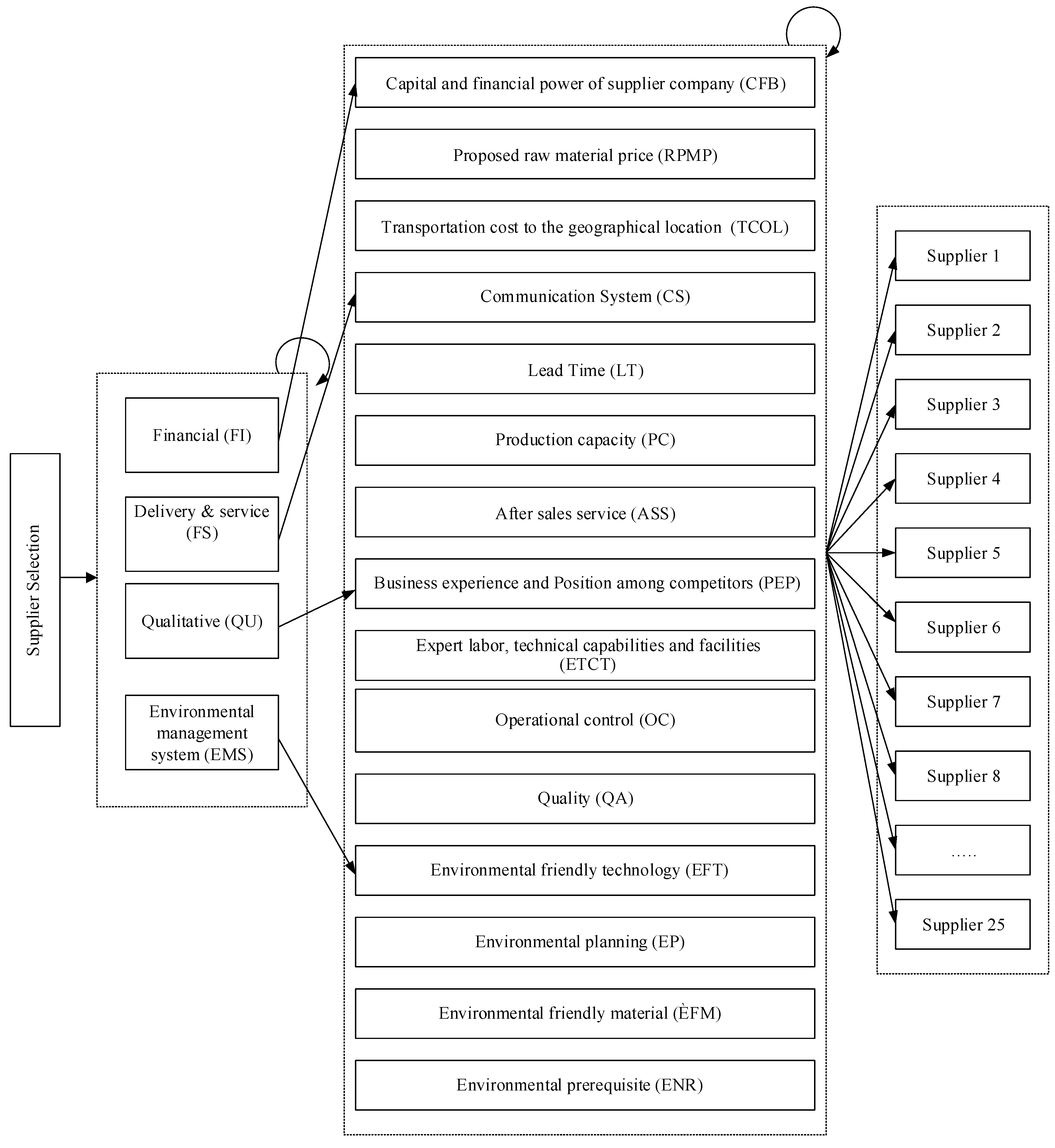
2.2. Criteria and Sub-Criteria for Supplier Selection

The initial criteria for the supplier set are developed based on a literature study.

Financial: The firm should require its suppliers to have a sound financial position. Financial strength can be a good indicator of the supplier’s long-term stability. A solid financial position also helps ensure that performance standards can be maintained and that products and services will continue to be available [48].

Delivery and service: A firm can use service performance criteria to evaluate the benefits provided by supplier services. When considering services, a firm needs to clearly define its expectations since there are few uniform, established service standards to draw upon. Since any purchase involves some degree of service, such as order processing, delivery, and support, a firm should always include some service criteria in its evaluation. If the supplier provides a solution combining products and services, the firm should be sure to adequately represent its service needs in the selection criteria [48]. The suppliers have to follow the predefined delivery schedule for achieving on-time delivery. All the manufacturers want to work with the supplier who can manage the supply chain system on time and has the ability for following the exact delivery schedule table [49].

Qualitative: Qualitative criteria are developed to measure important aspects of the supplier’s business: business experience and position among competitors, expert labor, technical capabilities and facilities, operational control, and quality [50].

Environmental management system: Due to increasing awareness about environmental degradation manufacturing companies and customers are both becoming alert of environmental protection [51]. This has led stakeholders of companies to ensure safe practices, like pollution control, reuse, recovery, etc. It includes criteria like pollution control: resource consumption of raw materials, use of environmentally friendly technology and materials, design capability for reduced consumption of materials/energy, reuse, and recycling of materials. To reduce the harm to the environment, organizations should also consider factors like permit requirements, compliance requirements, strategic considerations, climatic considerations, and government policy [52,53].

There are four main criteria and some sub-criteria, as shown in

Table 1. Criteria for supplier selection.

Criteria	Sub-Criteria	Researcher
Financial	Capital and financial power of supplier company	Ho et al. [54], Dickson [55], Weber et al. [56]
	Proposed raw material price	Banaeian et al. [50], Dickson [55], Weber et al. [56], Ho et al. [54]
	Transportation cost to the geographical location	Dickson [55], Weber et al. [56]
Delivery and service	Communication system	Dickson [55], Weber et al. [56]
	Lead time	Handfield [57], Choi & Hartley [58], Verma & Pullman [59], Bharadwa [60], Kannan et al. [61], Chu & Varma [62], Tam & Tummala [63], Shahgholian et al. [64]
	Production capacity	Kannan [61], Dickson [55], Weber et al. [56]
	After sales service	Dzever et al. [65], Choi & Hartley [58], Bevilacqua & Petroni [66], Bharadwaj [60], Rezaei & Ortt [67], Roshandel et al. [68]
Qualitative	Business experience and position among competitors	Banaeian et al. [50], Dickson [55], Weber et al. [56]
	Expert labor, technical capabilities and facilities	Banaeian et al. [50], Dickson [55], Weber et al. [56]
	Operational control	Dickson [55], Weber et al. [56]
	Quality	Grover et al. [55], Dickson [55]
Environmental management system	Environmental friendly technology	Rajesri Govindaraju et al. [69], Grover et al. [53]
	Environmental planning	Banaeian et al. [50], Nielsen et al. [70]
	Environmentally friendly material	Grover et al. [53]
	Environmental prerequisite	Banaeian et al. [50]

.

3. Material and Methodology

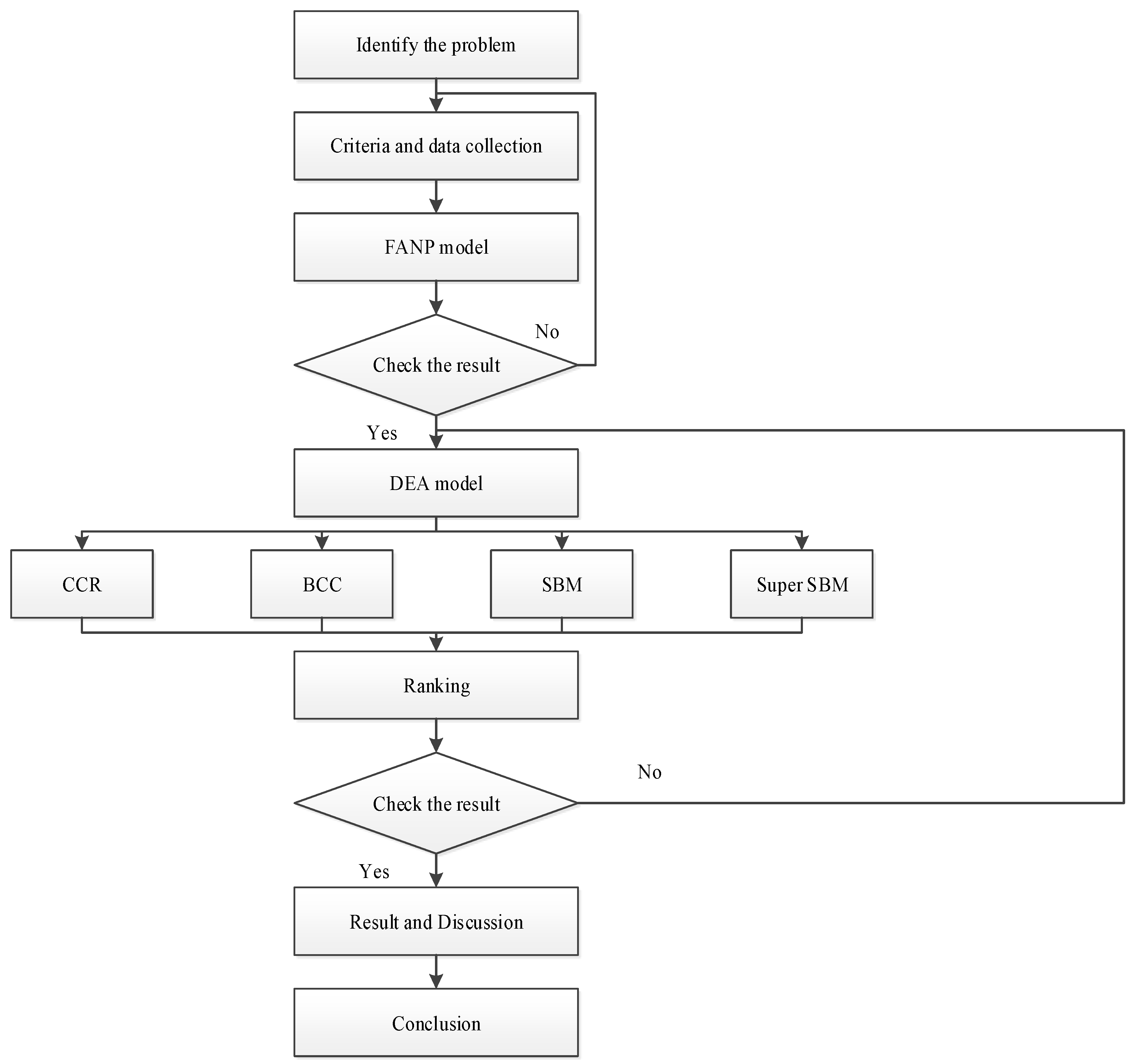
3.1. Research Development

Figure 1 illustrates the selection process, which is sequentially presented in three steps. In the first step, the decision-maker examines the material, interviews the experts, and surveys managers to determine the criteria and sub-criteria affecting to decision making. In the second step data are then processed using the FANP method to rank the criteria. Results from the FANP method are used for the input and output of the DEA model. The DEA model is implemented in the final stage.

Step 1: Determining evaluation criteria and sub-criteria

Determine the key criteria and sub-criteria for a comprehensive assessment of the potential supplier. At this stage, the identification of key criteria and sub-criteria is based on a review of the literature and scientific reports related to the content of the research to determine the necessary criteria for the topic [50]. After identifying the groups of criteria required, the decision-maker should select the potential supplier that matches the set criteria. Here, the criteria are defined as four main criteria and 15 sub-criteria, as shown in Figure 2.

Step 2: Implementing the FANP technique

Incorporating hybrid fuzzy set theory into the ANP model is the most effective tool for addressing complex problems of decision-making, which has a connection with various qualitative criteria [37]. As can be seen from the solution algorithm in this technique, as presented in Figure 3, at first, the decision-making hierarchical structure is determined to assist the selection [71].

Step 3: Implementation of the DEA model

In this study, the FANP and DEA techniques for efficiency measurement have advantages over other fuzzy ANP approaches. In this step, several DEA models, including the Charnes–Cooper–Rhodes model (CCR model), Banker–Charnes–Cooper model (BCC model), Slacks-Based Measure model (SBM model), and Super Slacks-Based Measure model (Super SBM model) are applied to rank suppliers and potential suppliers.

3.2. Methodology

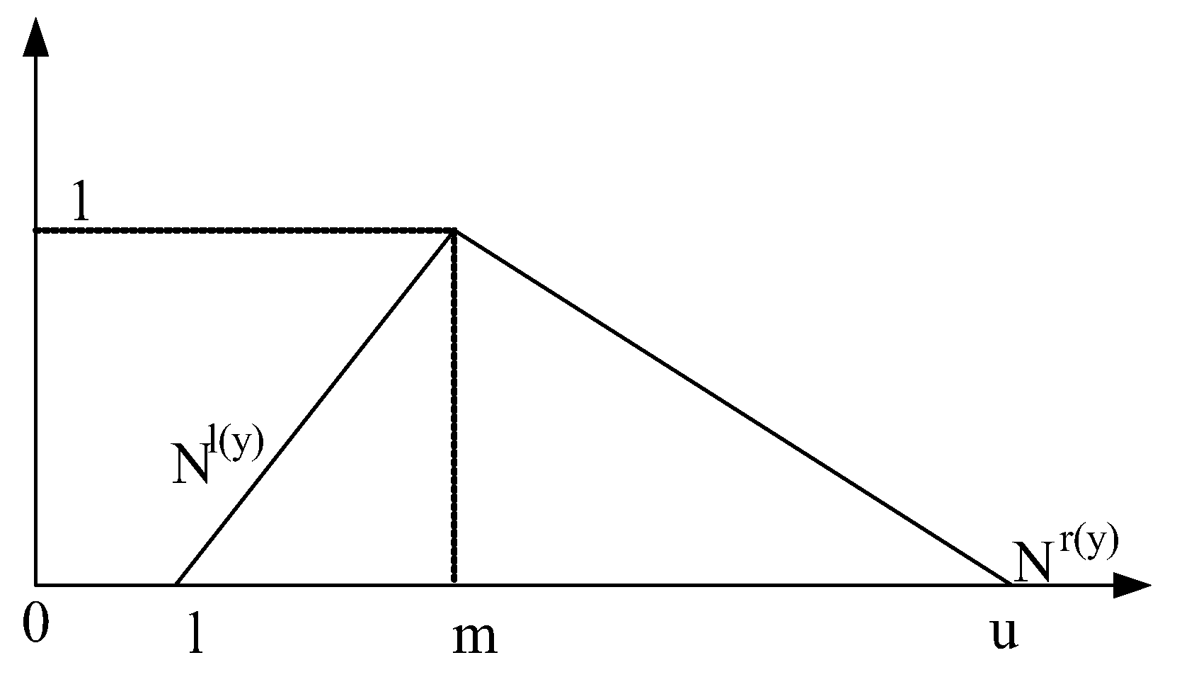
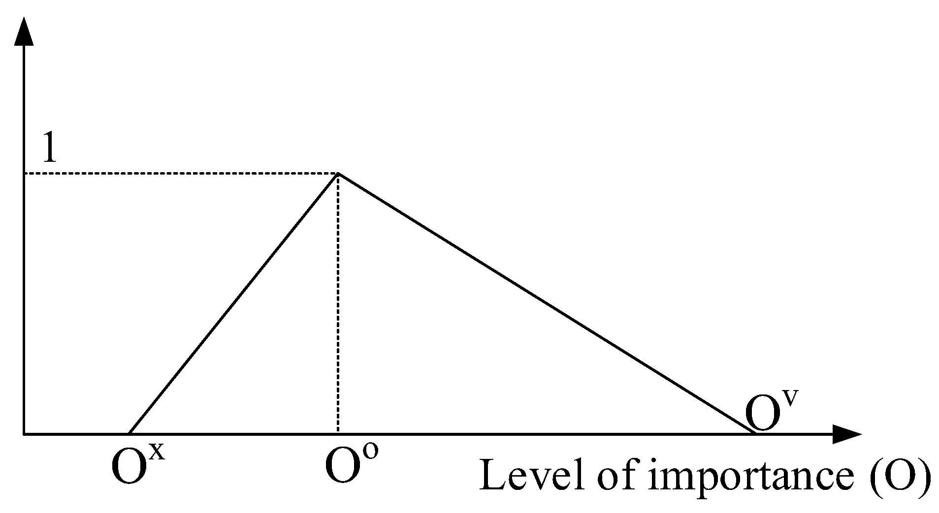
3.2.1. Fuzzy Set Theory

Fuzzy set was proposed by Zadeh to solve problems existing in uncertain environments. Fuzzy sets are functions that show the dependence degree of one fuzzy number on a set number. A tilde (~) is placed above any symbol representing a fuzzy set number. If $\tilde{A}$ is a TFN, each value of the membership function is between [0, 1] and can be explained, as shown in Equation (1):

$${\mu }_{\tilde{A}}(x)=\{\begin{array}{cc}\frac{(x-l)}{(m-l)}& l\le x\le m\\ \frac{(u-x)}{(u-m)}& m\le x\le u\\ 0& 0.W\end{array}$$

(1)

Each degree of membership includes a left- and right-side representation of a TFN, as shown here:

$$\tilde{N} =({\mathrm{N}}^{1(\mathrm{y})},{\mathrm{N}}^{\mathrm{r}(\mathrm{y})})=(1-(m-l)\mathrm{y},u+(m-u)\mathrm{y}),\mathrm{y}\in \left[0,1\right].$$

A TFN is shown in Figure 2.

3.2.2. Fuzzy Analytic Network Process

ANP does not require a strict hierarchical structure, such as AHP. It allows elements to control, and be controlled, by different levels or clusters of attributes. Several control elements are also present at the same level. Interdependence between factors and their level is defined as a systematic approach to feedback or interactions between elements.

During the ANP process, the elements will be compared pairwise using the expert rating scale, from which the weighting matrix is established. The weights are then adjusted by defining the product of the super matrix.

The AHP method provides a structured framework to set priorities for each level of the hierarchy by using pairwise comparisons quantitated with a priority scale of 1–9, as shown. In contrast, the ANP approach allows for more complex relationships between the elements and their ranks. The 1–9 scale for AHP is shown in

Table 2. The 1–9 scale for AHP [6].

Importance Intensity	Definition
1	Equally importance
3	Moderate importance
5	Strongly more importance
7	Very strong more importance
9	Extremely importance
2, 4, 6, 8	Intermediate values

.

It is clear that the disadvantage of ANP in dealing with the impression and objectiveness in the pairwise comparison process has been improved in the fuzzy analytic network process. The FANP applies a range of values to incorporate the decision-makers’ uncertainly [38], whereas the ANP model shows a crisp value. The author assigns the fuzzy conversion scale of this formula, which will be used in the Saaty [72] fuzzy prioritization approach, as shown in Table 2, where O_ab = (${\mathrm{O}}_{\mathrm{ab}}^{\mathrm{x}},{\mathrm{O}}_{\mathrm{ab}}^{\mathrm{o}},{\mathrm{O}}_{\mathrm{ab}}^{\mathrm{v}}$) is a triangular fuzzy number with the core ${\mathrm{O}}_{\mathrm{ab}}^{\mathrm{o}}$, the support [${\mathrm{O}}_{\mathrm{ab}}^{\mathrm{x}},{\mathrm{O}}_{\mathrm{ab}}^{\mathrm{v}}$], and the triangular fuzzy number, as shown in Figure 3.

The 1–9 fuzzy conversion scale is shown in

Table 3. The 1–9 fuzzy conversion scale [72].

Importance Intensity	Triangular Fuzzy Scale
1	(1, 1, 1)
2	(1, 1, 2)
3	(1, 2, 3)
4	(2, 3, 4)
5	(3, 4, 5)
6	(4, 5, 6)
7	(5, 6, 7)
8	(7, 8, 9)
9	(9, 9, 9)

:

The reversed degree to O_ab expressing the non-preference is also expressed by a triangular fuzzy number: (1/$O_{ab}^v$, 1/$O_{ab}^o,1/O_{ab}^x$. ). By the way, the weights of criteria from the fuzzy Saaty’s matrix can be divided into four steps [73]:

• Fuzzy synthetic extension calculation will transformed into TNT, called fuzzy synthetic extensions $K_a(k_a^x,k_a^o,k_a^{uv})$. using Equations (2)–(4) [74]:

  $$K_a={\sum }_{b=1}^n{O}_{ab}⨂{({\sum }_{a=1}^n{\sum }_{b=1}^n{O}_{ab})}^{-1}$$

  (2)

  $${\displaystyle \sum }_{j=1}^n{O}_{ab}=\left({\displaystyle \sum }_{b=1}^n{M}_{ab}^x,{\displaystyle \sum }_{j=1}^n{O}_{ab}^o,{\displaystyle \sum }_{b=1}^n{O}_{ab}^v\right)$$

  (3)

  $$O_{ab}^{-1}=1/O_{ab}^v,1/O_{ab}^o,1/O_{ab}^x$$

  (4)

  $$O⨂\mathrm{N}=(O_x . N_x, O_0. N_0, O_v.N_v)$$

  (5)

  Assign a = 1, 2, …, n, in which a and b specifically are triangular fuzzy number (O_x, O_o, O_v) and (N_x, N₀, N_v).
• Weights of criteria are addressed by using relations of the fuzzy-valued. In this step, fuzzy synthetic extensions are blurred by using the min fuzzy extension of the valued relation ≤ given by Equation (5), and weights W_i are calculated (for more detail, see [75]):

  $${\mathrm{Q}}_{\mathrm{a}}=mi{n}_b\left\{\frac{k_b^b-k_a^v}{(k_a^o-k_a^v)-(k_b^o-k_b^x)}\right\}$$

  (6)

  For a, b = 1, 2, …., n.
• The standardization of the weights. If we expect to obtain the sum of weights within one matrix equal to 1, final weights w_i are solved using Equation (7):

  $$q_i=Q_i/{\sum }_{a=1}^n{Q}_a$$

  (7)

  For a, b = 1, 2, …, n.
• An assessment of a Saaty’s matrix consistency. In the line with [74], a consistency of the matrix is sufficient if inequality from Equation (8) holds:

  $$RT= \frac{CT}{RR}=\frac{\overline{\lambda }-n}{(n-1).RR}\le 0.1$$

  (8)

  where $\overline{\lambda }$ is a symbol for the arithmetic mean of the maximum real eigenvalues of the matrices ${(a_{ab}^{\xi })}_{1\le a,b\le n},\xi \in \left\{x,o,v\right\}$ for a, b = 1, 2, ..., n is the size of the Saaty’s matrix, and RR represents a random index whose value depends on [74].

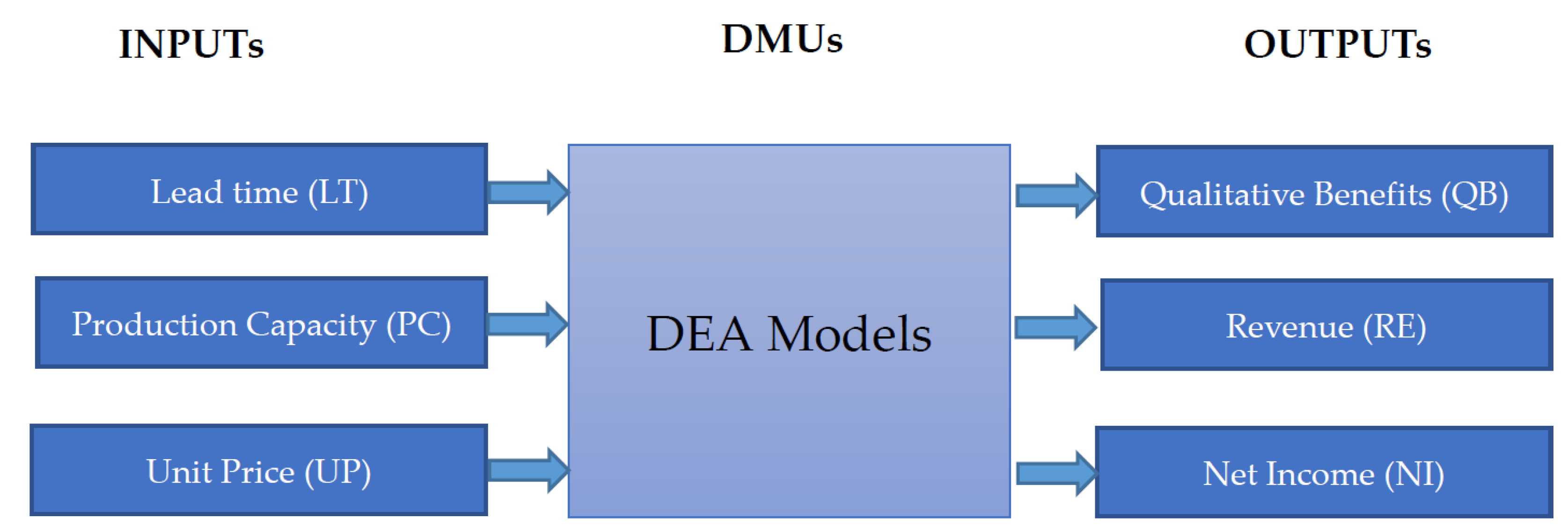
3.3. Data Envelopment Analysis

3.3.1. Charnes-Cooper-Rhodes Model (CCR Model)

Charnes, Cooper, and Rhodes (1978) [30] proposed a basic DEA model, called the CCR model:

$$\begin{array}{cc}& \underset{f.g}{\max }\mathsf{\gamma }=\frac{f^V{y}_0}{g^V{x}_0}\\ \mathrm{S}.\mathrm{t}.& \\ & f^V{y}_{b }-g^V{x}_b\le 0,b=1,2,\dots ,n\\ & f\ge 0\\ & g\ge 0\end{array}$$

(9)

Due to constraints, the optimal value $\mathsf{\gamma }$* is a maximum of 1.

DMU₀ is efficient if ${\gamma }^{*}=1$ and have at least one optimal f* > 0 and g* > 0. In addition, the fractional program can be presented as follows [76]:

$$\begin{array}{cc}& \underset{g.f}{\min }\gamma =g^v{y}_0\\ \mathrm{S}\mathrm{t}.& \\ & g^v{x}_0-1=0\\ & f^v{y}_j-g^v{x}_j\le 0, j=1, 2,\cdots ,n\\ & g\ge 0\\ & f\ge 0\end{array}$$

(10)

The Farrell [77] model of Equation (10) with variable $\gamma$ and a nonnegative vector $\beta ={\beta }_1,{\beta }_2,{\beta }_3,\dots ,{\beta }_n$ is expressed as [76].

$$\begin{array}{cc}& max{\displaystyle \sum _{i=1}^m}{d}_i^{-}+{\displaystyle \sum _{r=1}^s}{d}_r^{+}\\ \mathrm{S}.\mathrm{t}& \\ & {\displaystyle \sum _{j=1}^n}{x}_{ij}{\beta }_j+d_i^{-}=\gamma x_{i0},i=1,2,\dots ,p\\ & {\displaystyle \sum _{j=1}^n}{y}_{rj}{\beta }_j-d_r^{+}=y_{r0},r=1,2,\dots ,q\\ & {\beta }_j\ge 0,j=1,2,\dots ,n\\ & d_i^{-}\ge 0,i=1,2,\dots ,p\\ & d_r^{+}\ge 0,r=1,2,\dots ,q\end{array}$$

(11)

Equation (11) has a feasible solution, ${\gamma }^{*}=1,{\beta }_0^{*}=1,{\beta }_j^{*}=0,(j\ne 0),\mathrm{which}$ effects the optimal value ${\gamma }^{*}$ not greater than 1. The process will be repeated for each DMUj, j = 1, 2, …, n. DMUs are inefficient when ${\gamma }^{*}$ < 1, while DMUs are boundary points if ${\gamma }^{*}=1$. We avoid the weakly efficient frontier point by invoking a linear program as follows [76]:

$$\begin{array}{cc}& max{\displaystyle \sum _{i=1}^m}{d}_i^{-}+{\displaystyle \sum _{r=1}^d}{d}_r^{+}\\ \mathrm{S}.\mathrm{t}& \\ & {\displaystyle \sum _{j=1}^n}{x}_{ij}{\beta }_j+d_i^{-}=\gamma x_{i0},i=1,2,\dots ,p\\ & {\displaystyle \sum _{j=1}^n}{y}_{rj}{\beta }_j-d_r^{+}=y_{r0},r=1,2,\dots ,q\\ & {\beta }_j\ge 0,j=1,2,\dots ,n\\ & d_i^{-}\ge 0,i=1,2,\dots ,p\\ & d_r^{+}\ge 0,r=1,2,\dots ,q\end{array}$$

(12)

In this case, note that the choices the $d_i^{-}$ and $d_r^{+}$ do not affect the optimal ${\gamma }^{*}$. The performance of DMU₀ achieves 100% efficiency if, and only if, both (1) ${\gamma }^{*}=1$ and (2) $d_i^{-*}$ = $d_r^{+}=0.$ The performance of DMU₀ is weakly efficient if, and only if, both (1)${\gamma }^{*}=1$ and (2) $d_i^{-*}\ne 0$ and $d_r^{+}\ne 0$ for i or r in optimal alternatives. Thus, the preceding development amounts to solving the problem as follows [76]:

$$\begin{array}{cc}& min\theta -\alpha \left({\displaystyle \sum _{i=1}^m}{d}_i^{-}+{\displaystyle \sum _{r=1}^d}{d}_r^{+}\right)\\ \mathrm{S}.\mathrm{t}& \\ & {\displaystyle \sum _{j=1}^n}{x}_{ij}{\beta }_j+d_i^{-}=\gamma x_{i0},i=1,2,\dots ,p\\ & {\displaystyle \sum _{j=1}^n}{y}_{rj}{\beta }_j-d_r^{+}=y_{r0},r=1,2,\dots ,q\\ & {\beta }_j\ge 0,j=1,2,\dots ,n\\ & d_i^{-}\ge 0,i=1,2,\dots ,p\\ & d_r^{+}\ge 0,r=1,2,\dots ,q\end{array}$$

(13)

In this case, $d_i^{-}$ and $d_r^{+}$ variables will be used to convert the inequalities into equivalent equations. This is similar to solving Equation (11) in two stages by first minimizing $\gamma$ and then fixing $\gamma ={\gamma }^{*}$ as in Equation (12). This would reset the objective from max to min, as in Equation (9), to obtain [76]:

$$\begin{array}{cc}& \underset{g.f}{\max }\gamma =\frac{g^V{x}_0}{f^V{y}_j}\\ \mathrm{S}.\mathrm{t}& \\ & g^V{x}_0\le g^V{y}_j,j=1,2,\dots ,n\\ & g\ge \epsilon >0\\ & f\ge \epsilon >0\end{array}$$

(14)

If the α > 0 and the non-Archimedean element is defined, the input models are similar to Equations (10) and (13), as follows [76]:

$$\begin{array}{cc}& \underset{g.f}{\max }\gamma =g^V{x}_0\\ \mathrm{S}.\mathrm{t}& \\ & f^V{y}_0=1\\ & g^V{x}_o-f^V{y}_j\ge 0, j=1, 2,\dots ,n\\ & g\ge \epsilon >0\\ & f\ge \epsilon >0\end{array}$$

(15)

and:

$$\begin{array}{cc}& max\varphi -\epsilon \left({\displaystyle \sum _{i=1}^m}{d}_i^{-}+{\displaystyle \sum _{r=1}^d}{d}_r^{+}\right)\\ \mathrm{S}.\mathrm{t}& \\ & {\displaystyle \sum _{j=1}^n}{x}_{ij}{\beta }_j+d_i^{-}=x_{i0},i=1,2,\dots ,p\\ & {\sum }_{j=1}^n{y}_{rj}{\beta }_j-d_r^{+}=\varnothing y_{r0},r=1,2,\dots ,q\\ & {\beta }_j\ge 0,j=1,2,\dots ,n\\ & d_i^{-}\ge 0,i=1,2,\dots ,p\\ & d_r^{+}\ge 0,r=1,2,\dots ,q\end{array}$$

(16)

The input-oriented CCR (CCR-I) has the dual multiplier model, expressed as [76]:

$$\begin{array}{cc}& \max z={\displaystyle \sum _{r=1}^q}{g}_r{y}_{r0}\\ \mathrm{S}.\mathrm{t}& \\ & {\displaystyle \sum _{r=1}^q}{g}_r{y}_{rj}-{\displaystyle \sum _{r=1}^q}{f}_r{y}_{rj}\le 0\\ & {\displaystyle \sum _{i=1}^p}{f}_i{x}_{i0}=1\\ & g_r,f_i\ge \epsilon >0\end{array}$$

(17)

The output-oriented CCR (CCR-O) has the dual multiplier model, expressed as [76]:

$$\begin{array}{cc}& \min q={\displaystyle \sum _{i=1}^p}{f}_i{x}_{i0}\\ \mathrm{S}.\mathrm{t}& \\ & {\displaystyle \sum _{i=1}^p}{f}_i{x}_{ij}-{\displaystyle \sum _{r=1}^q}{g}_r{y}_{rj}\le 0\\ & {\displaystyle \sum _{r=1}^q}{g}_r{y}_{r0}=1\\ & g_r,f_i\ge \epsilon >0\end{array}$$

(18)

3.3.2. Banker–Charnes–Cooper Model (BCC Model)

Banker et al. proposed the input-oriented BBC model (BCC-I) [30], which is able to assess the efficiency of DMU₀ by solving the following linear program [76]:

$$\begin{array}{cc}& {\gamma }_B=min\gamma \\ \mathrm{S}.\mathrm{t}& \\ & {\displaystyle \sum _{j=1}^n}{x}_{ij}{\beta }_j+d_i^{-}=\gamma x_{i0},i=1,2,\dots ,p\\ & {\displaystyle \sum _{j=1}^n}{y}_{rj}{\beta }_j-d_r^{+}=y_{r0},r=1,2,\dots ,q\\ & {\displaystyle \sum _{k=1}^n}{\beta }_k=1\\ & {\beta }_k\ge 0,k=1,2,\dots ,n\end{array}$$

(19)

We avoid the weakly efficient frontier point by invoking the linear program as follows [76]:

$$\begin{array}{cc}& max{\displaystyle \sum _{i=1}^m}{d}_i^{-}+{\displaystyle \sum _{r=1}^d}{d}_r^{+}\\ \mathrm{S}.\mathrm{t}& \\ & {\displaystyle \sum _{j=1}^n}{x}_{ij}{\beta }_j+d_i^{-}=\gamma x_{i0},i=1,2,\dots ,p\\ & {\displaystyle \sum _{j=1}^n}{y}_{rj}{\beta }_j-d_r^{+}=y_{r0},r=1,2,\dots ,q\\ & {\displaystyle \sum _{k=1}^n}{\beta }_k=1\\ & {\beta }_k\ge 0,k=1,2,\dots ,n\\ & d_i^{-}\ge 0,i=1,2,\dots ,p\\ & d_r^{+}\ge 0,r=1,2,\dots ,q\end{array}$$

(20)

Therefore, this is the first multiplier form to solve the problem as follows [76]:

$$\begin{array}{cc}& min\gamma -\epsilon \left({\displaystyle \sum _{i=1}^m}{d}_i^{-}+{\displaystyle \sum _{r=1}^d}{d}_r^{+}\right)\\ \mathrm{S}.\mathrm{t}& \\ & {\displaystyle \sum _{j=1}^n}{x}_{ij}{\beta }_j+d_i^{-}=\gamma x_{i0},i=1,2,\dots ,p\\ & {\displaystyle \sum _{j=1}^n}{y}_{rj}{\beta }_j-d_r^{+}=y_{r0},r=1,2,\dots ,q\\ & {\displaystyle \sum _{k=1}^n}{\beta }_k=1\\ & {\beta }_k\ge 0,k=1,2,\dots ,n\\ & d_i^{-}\ge 0,i=1,2,\dots ,p\\ & d_r^{+}\ge 0,r=1,2,\dots ,q\end{array}$$

(21)

The linear program in Equation (17) gives us the second multiplier form, which is expressed as [76]:

$$\begin{array}{cc}& \underset{g.f,f_0}{\max }{\gamma }_B=f^V{y}_0-f_0\\ \mathrm{S}.\mathrm{t}& \\ & g^V{x}_0=1\\ & f^V{y}_j-g^V{x}_j-f_0\le 0, j=1, 2,\dots ,n\\ & g\ge 0\\ & f\ge 0\end{array}$$

(22)

If g and f, which are mentioned in Equation (22), are vectors, the scalar $v_0$ may be positive or negative (or zero). Thus, the equivalent BCC fractional program is obtained from the dual program in Equation (22) as [76]:

$$\begin{array}{cc}& \underset{g.f}{\max }\gamma =\frac{f^V{y}_0-f_0}{g^V{x}_0}\\ \mathrm{S}.\mathrm{t}& \\ & \frac{f^V{y}_j-f_0}{g^V{x}_j}\le 1,j=1,2,\dots ,n\\ & g\ge 0\\ & f\ge 0\end{array}$$

(23)

The DMU₀ can be called BCC-efficient if an optimal solution $({\gamma }_B^{*},d^{-*},d^{+*})\mathrm{is}$ claimed in this two-phase process for Equation (17) satisfies ${\gamma }_B^{*}=1$ and has no slack $d^{-*}=d^{+*}$ = 0, then. The improved activity $({\gamma }^{*}x-d^{-*},y+d^{+*})$ also can be illustrated as BCC-efficient [76].

The output-oriented BCC model (BCC–O) is:

$$\begin{array}{cc}& \max \eta \\ \mathrm{S}.\mathrm{t}& \\ & {\displaystyle \sum _{j=1}^n}{x}_{ij}{\beta }_j+d_i^{-}=\gamma x_{i0},i=1,2,\dots ,p\\ & {\displaystyle \sum _{j=1}^n}{y}_{rj}{\beta }_j-d_r^{+}=\eta y_{r0},r=1,2,\dots ,q\\ & {\displaystyle \sum _{k=1}^n}{\beta }_k=1\\ & {\beta }_k\ge 0,k=1,2,\dots ,n\end{array}$$

(24)

From Equation (24), we have the associate multiplier form, which is expressed as [76]:

$$\begin{array}{cc}& \underset{g.f,g_0}{\min }{f}^V{y}_0-f_0\\ \mathrm{S}.\mathrm{t}& \\ & f^V{y}_0=1\\ & g^V{x}_j-f^V{y}_j-f_0\le 0,j=1,2,\dots ,n\\ & g\ge 0\\ & f\ge 0\end{array}$$

(25)

f₀ is the scalar associated with ${{\displaystyle \sum }}_{k=1}^n{\beta }_k=1$. In conclusion, the authors achieve the equivalent (BCC) fractional programming formulation for Equation (25) [76]:

$$\begin{array}{cc}& \underset{g.f,g_0}{\min }\frac{g^V{x}_0-f_0}{f^V{y}_0}\\ \mathrm{S}.\mathrm{t}& \\ & \frac{f^V{x}_j-f_0}{f^V{y}_j}\le 1,j=1,2,\dots ,n\\ & g\ge 0\\ & f\ge 0\end{array}$$

(26)

3.3.3. Slacks-Based Measure Model (SBM Model)

The SBM model was introduced by Tone [78] (see also Pastor et al. [79]).

Input-Oriented SBM (SBM-I-C)

The input-oriented SBM under a constant-returns-to-scale assumption [76] is described as follows:

$$\begin{array}{cc}& {\rho }_I^{*}=\underset{\beta , d^{-},d^{+}}{\min }1-\frac{1}{m}{\displaystyle \sum _{i=1}^m}\frac{d_i^{-}}{x_{ih}}\\ \mathrm{S}.\mathrm{t}& \\ & x_{ic}={\displaystyle \sum _{j=1}^m}{x}_{ic}{\beta }_i+d_i^{-},i=1,2,\dots m\\ & y_{rc}={\displaystyle \sum _{j=1}^m}{y}_{rc}{\beta }_i-d_r^{+},i=1,2,\dots d\\ & {\beta }_j\ge 0,k(\forall j),d_i^{-}\ge 0(\forall j),d_r^{+}\ge 0(\forall j)\end{array}$$

(27)

The DMUs in the reference set R of $(x_c,y_c)$ are SBM-input-efficient. In addition, the SBM-input-efficiency score must is lower than the CCR efficiency score.

Output-Oriented SBM (SBM-O-C)

The output-oriented SBM efficiency ${\rho }_O^{*}$ of DMU_c = (x_c, y_c) is defined by [SBM-O-C] [76]:

$$\begin{array}{cc}& \raisebox{1ex}{$1$}\!\left/ \!\raisebox{-1ex}{${\rho }_O^{*}$}\right.=\underset{\lambda ,s^{-},s^{+}}{\max }1+\frac{1}{s}{{\displaystyle \sum }}_{r=1}^s\frac{s_r^{+}}{y_{rh}}\\ \mathrm{S}.\mathrm{t}.& \\ & x_{ic}={\displaystyle \sum _{j=1}^n}{x}_{ij}{\beta }_j+ d_j^{-}(i=1,..m)\\ & y_{ic}={\sum }_{j=1}^n{y}_{ij}{\beta }_j+d_i^{+}(i=1,\dots m)\\ & {\beta }_j\ge 0(\forall j), d_i^{-}\ge 0(\forall i), d_i^{+}\ge 0 (\forall r)\\ \mathrm{The} \mathrm{optimal} \mathrm{solution}& \mathrm{of} [\mathrm{SBM}-\mathrm{O}-\mathrm{C}]{\beta }^{*},d^{-*},d^{+*}).\end{array}$$

(28)

3.3.4. Super-Slacks-Based Measure Model (Super SBM Model)

Tone’s super SBM model [78] has proposed a slacks-based measure of efficiency (SBM model) that measures the efficiency of the units under evaluation using slack variables only. The super efficiency SBM model removes the evaluated unit DMUq from the set of units and looks for a DMU* with inputs x_i*, i = 1, ..., m, and outputs y_k*, k = 1, ..., r, being SBM (and CCR) efficient after this removal. The super SBM model is formulated as follow:

$$\begin{array}{cc}\mathrm{minimize} {\theta }_q^{SBM}=& \frac{\frac{1}{p}{{\displaystyle \sum }}_{i=1}^m{x}_i^{*}/x_{i0}}{\frac{1}{q}{{\displaystyle \sum }}_{k=1}^r{y}_k^{*}/y_{k0}}\\ & \mathrm{S}.\mathrm{t}\end{array}$$

(29)

$$\begin{gathered} {\displaystyle \sum _{j=1}^n}{x}_{ij}{\beta }_j+d_i^{-}=\gamma x_{i0},i=1,2,\dots ,p \\ {\displaystyle \sum _{j=1}^n}{y}_{rj}{\beta }_j-d_r^{+}=y_{r0},r=1,2,\dots ,q \\ {x}_i^{*}\ge x_{i0},i=1,2,\dots ,n \\ {y}_k^{*}\le y_{k0},k=1,2,\dots ,n \\ {\beta }_k\ge 0,k=1,2,\dots ,n \\ {d}_i^{-}\ge 0,i=1,2,\dots ,p \\ {d}_r^{+}\ge 0,r=1,2,\dots ,q \end{gathered}$$

(30)

The numerator in the ratio in Equation (29) can be explained as the distance of units DMUq and DMU* in input space and the average reduction rate of inputs of DMU* to inputs of DMUq.

4. Case Study

In this research, the authors collected 25 suppliers (DMU) in Vietnam. Information about the suppliers is shown in

Table 4. Number of suppliers (DMU).

No	Company Name	Address	Turnover (USD)	Employees	Market Geographical Area	Symbol
1	An Gia Phu Food and Cereal Limited Liability Company	Vinh Long Province, Vietnam	616,894	25	Vietnam	DMU 1
2	VINA Fragrant Rice Limited Liability Company	Can Tho City, Vietnam	877,662	39	Vietnam	DMU 2
3	Thai Hung Cereal Co-operative Company	Can Tho City, Vietnam	616,309	31	Vietnam	DMU 3
4	Sang Mai Agricultural Production Limited Liability Company	Hai Phong Provice, Vietnam	686,350	39	Vietnam	DMU 4
5	FAS Vietnam Cereal Limited Liability Company	Vinh Long Province, Vietnam	729,349	24	Vietnam	DMU 5
6	S1000 Food Commercial and Service Limited Liability Company	Ho Chi Minh City, Vietnam	590,814	21	Vietnam	DMU 6
7	Khau Thien Thanh Phat Production and Commercial Export-Import Company	Ho Chi Minh City, Vietnam	3,180,926	121	Vietnam, Malaysia, Japan, Australia	DMU 7
8	Gia Son Phat Commercial and Service Limited Liability Company	Kien Giang, Vietnam	613,654	33	Vietnam	DMU 8
9	VILACONIC Cereal Joint Stock Company	Nghe An Province, Vietnam	717,780	31	Vietnam	DMU 9
10	Binh Minh Cereal Joint Stock Company	Can Tho City, Vietnam	658,272	26	Vietnam	DMU 10
11	Phu Thai Huong Joint Stock Company	Long An Province, Vietnam	1.347,621	57	Vietnam	DMU 11
12	Long Tra Agroforestry Food Production Limited Liability Company	Ho Chi Minh City, Vietnam	4,650,698	234	Vietnam, Asia	DMU 12
13	Huong Chien Rice Production Limited Liability Company	Long An Province, Vietnam	674,388	18	Vietnam	DMU 13
14	Loc Troi Joint Stock Incorporated Company	An Giang Province, Vietnam	3,077,786	179	Vietnam, Lao, Cambodia	DMU 14
15	Ngoc Oanh Rice Private Business	Ho Chi Minh City, Vietnam	502,448	23	Vietnam	DMU 15
16	Khanh Tam Rice Private Business	Ho Chi Minh City Vietnam	589,577	16	Vietnam	DMU 16
17	Thien Ngoc Cereal Limited Liability Company	Long An Province, Vietnam	1,094,880	31	Vietnam	DMU 17
18	Xuyen Giang Commercial and Service Limited Liability Company	Ho Chi Minh City, Vietnam	1,475,431	59	Vietnam	DMU 18
19	Viet Lam Commercial and Service Limited Liability Company	Vinh Long Province, Vietnam	1,502,043	42	Vietnam	DMU 19
20	Long An Export-Production Joint Stock Company	Ha Noi City, Vietnam	2,125,825	89	Vietnam, EU	DMU 20
21	Phat Tai Limited Liability Company	Dong Thap Province, Vietnam	1,054,156	29	Vietnam	DMU 21
22	Thai Binh Rice Joint Stock Company	Thai Binh Province, Vietnam	1,777,244	51	Vietnam	DMU 22
23	Angimex Kitoku Limited Liability Company	Tien Giang Province, Vietnam	1,098,978	38	Vietnam	DMU 23
24	Hoa Lua Rice Commercial Limited Liability Company	Ho Chi Minh City, Vietnam	1,029,622	59	Vietnam	DMU 24
25	Phuong Quan Production Limited Liability Company	Long An Province, Vietnam	1,733,256	61	Vietnam	DMU 25

.

The data collection of the FANP and hierarchical structure are introduced in Figure 4.

A fuzzy comparison matrix for all criteria is shown in

Table 5. Fuzzy comparison matrix for criteria.

Criteria	FS	EMS	FI	QU
FS	(1, 1, 1)	(1/8, 1/7, 1/6)	(1/9, 1/8, 1/7)	(1/3, 1/2, 1)
EMS	(6, 7, 8)	(1, 1, 1)	(1/6, 1/5, 1/4)	(1, 2, 3)
FI	(7, 8, 9)	(4, 5, 6)	(1, 1, 1)	(4, 5, 6)
QU	(1, 2, 3)	(1/3, 1/2, 1)	(1/6, 1/5, 1/4)	(1, 1, 1)

.

During the defuzzification, we obtain the coefficients α = 0.5 and β = 0.5 (Tang and Beynon) [80]. In it, α represents the uncertain environment conditions, and β represents the attitude of the evaluator is fair.

$$\begin{gathered} {\mathrm{g}}_{0.5,0.5}(\overline{a_{EMS,FS}}) = \left[(0.5 \times 6.5) + (1 - 0.5) \times 7.5\right] = 7 \\ {\mathrm{f}}_{0.5}(L_{EMS,FS}) = (7 - 6) \times 0.5 + 6 = 6.5 \\ {\mathrm{f}}_{0.5}(U_{EMS,FS}) = 8 - (8 - 7) \times 0.5 = 7.5 \\ {\mathrm{g}}_{0.5,0.5}(\overline{a_{EMS,FS}}) =1/7 \end{gathered}$$

The remaining calculations are similar to the above, as well as the fuzzy number priority points. The real number priorities when comparing the main criteria pairs are presented in

Table 6. Real number priority.

Criteria	FS	EMS	FI	QU
FS	1	1/7	1/8	1/2
EMS	7	1	1/6	2
FI	8	6	1	5
QU	2	1/2	1/5	1

.

We calculate the maximum individual values as follows:

$$\begin{gathered} GM1={(1\times 1/7\times 1/8\times 1/2)}^{1/4}=0.03073 \\ GM2={(7\times 1\times 1/6\times 2)}^{1/4}=1.2359 \\ GM3={(8\times 6\times 1\times 5)}^{1/4}=3.9359 \\ GM4={(2\times 1/2\times 1/5\times 1)}^{1/4}=0.6687 \\ \sum GM=GM1+GM2+GM3+GM4=6.1478 \end{gathered}$$

$$\begin{gathered} {\omega }_1=\frac{0.3073}{6.1478}=0.0499 \\ {\omega }_2=\frac{1.2359}{6.1478}=0.2010 \\ {\omega }_3=\frac{3.9359}{6.1478}=0.6402 \\ {\omega }_4=\frac{0.6687}{6.1478}=0.1087 \end{gathered}$$

$$\begin{gathered} \left[\begin{array}{c}\begin{array}{ccc}1& 1/7& \begin{array}{cc}1/8& 1/2\end{array}\end{array}\\ \begin{array}{ccc}7& 1& \begin{array}{cc}1/6& 2\end{array}\end{array}\\ \begin{array}{c}\begin{array}{cc}8& \begin{array}{ccc}6& 1& 5\end{array}\end{array}\\ \begin{array}{ccc}2& 1/2& \begin{array}{cc}1/5& 1\end{array}\end{array}\end{array}\end{array}\right]\times \left[\begin{array}{c}0.0499\\ 0.2010\\ \begin{array}{c}0.6402\\ 0.1087\end{array}\end{array}\right]=\left[\begin{array}{c}0.2129\\ 0.8744\\ \begin{array}{c}2.7889\\ 0.4370\end{array}\end{array}\right] \\ \left[\begin{array}{c}0.2129\\ 0.8744\\ \begin{array}{c}2.7889\\ 0.4370\end{array}\end{array}\right]/\left[\begin{array}{c}0.0499\\ 0.2010\\ \begin{array}{c}0.6402\\ 0.1087\end{array}\end{array}\right]=\left[\begin{array}{c}4.2665\\ 4.3502\\ \begin{array}{c}4.3562\\ 4.0202\end{array}\end{array}\right] \end{gathered}$$

with the number of criteria is 4, we obtain n = 4, and λ_max and CI are calculated as follows:

$${\lambda }_{max}=\frac{4.2665+4.3502+4.3562+4.0202}{4}=4.2482$$

$$CI=\frac{4.2482-4}{4-1}=0.0827$$

For CR, with n = 4 we obtain RI = 0.9:

$$CR=\frac{0.0827}{1.12}=0.0919$$

We have CR = 0.0919 ≤ 0.1, so the pairwise comparison data is consistent and does not need to be re-evaluated. The results of the pair comparison between the main criteria are presented in

Table 7. Fuzzy comparison matrices for the criteria.

Criteria	FS	EMS	FI	QU	Weight
FS	(1, 1, 1)	(1/8, 1/7, 1/6)	(1/9, 1/8, 1/7)	(1/3, 1/2, 1)	0.04929
EMS	(6, 7, 8)	(1, 1, 1)	(1/7, 1/6, 1/5)	(1, 2, 3)	0.20144
FI	(7, 8, 9)	(5, 6, 7)	(1, 1, 1)	(4, 5, 6)	0.64816
QU	(1, 2, 3)	(1/3, 1/2, 1/1)	(1/6, 1/5, 1/4)	(1, 1, 1)	0.10111
Total					1
CR = 0.09480

,

Table 8. Comparison matrix for the financial criteria.

Criteria	CFB	RPMP	TCOOL	Weight
CFB	(1, 1, 1)	(1/5, 1/4, 1/3)	(3, 4, 5)	0.2290
RPMP	(3, 4, 5)	(1, 1, 1)	(6, 7, 8)	0.6955
TCOOL	(1/5, 1/4, 1/3)	(1/8, 1/7, 1/6)	(1, 1, 1)	0.0754
Total				1
CR = 0.07348

,

Table 9. Comparison matrix for the delivery and service criteria.

Criteria	CS	LT	PC	ASS	Weight
CS	(1, 1, 1)	(1/9, 1/8, 1/7)	(1/5, 1/4, 1/3)	(2, 3, 4)	0.0924
LT	(7, 8, 9)	(1, 1, 1)	(1/3, 1/2, 1)	(6, 7, 8)	0.3956
PC	(3, 4, 5)	(1, 2, 3)	(1, 1, 1)	(7, 8, 9)	0.4672
ASS	(1/4, 1/3, 1/2)	(1/8, 1/7, 1/6)	(1/9, 1/8, 1/7)	(1, 1, 1)	0.0448
Total					1
CR = 0.09456

,

Table 10. Comparison matrix for the qualitative criteria.

Criteria	PEP	ETCT	OC	QA	Weight
PEP	(1, 1, 1)	(2, 3, 4)	(4, 5, 6)	(1/5, 1/4, 1/3)	0.2136
ETCT	(1/4, 1/3, 1/2)	(1, 1, 1)	(1/4, 1/3, 1/2)	(1, 1, 1)	0.0436
OC	(1/6, 1/5, 1/4)	(2, 3, 4)	(1, 1, 1)	(1/9, 1/8, 1/7)	0.0791
QA	(3, 4, 5)	(1, 1, 1)	(7, 8, 9)	(1, 1, 1)	0.6638
Total					1
CR = 0.09005

and

Table 11. Comparison matrix for the environmental management systems criteria.

Criteria	EFT	EP	EFM	ENR	Weight
EFT	(1, 1, 1)	(1/9, 1/9, 1/9)	(1/6, 1/5, 1/4)	(1/6, 1/5, 1/4)	0.0445
EP	(9, 9, 9)	(1, 1, 1)	(1, 2, 3)	(5, 6, 7)	0.5345
EFM	(4, 5, 6)	(1/3, 1/2, 1)	(1, 1, 1)	(3, 4, 5)	0.3009
ENR	(4, 5, 6)	(1/7, 1/6, 1/5)	(1/5, 1/4, 1/3)	(1, 1, 1)	0.1201
Total					1
CR = 0.0838

.

Based on how the hierarchical structure was built, the pairwise comparison matrix was built through completing a questionnaire. Then, the received data to calculate the weight of supplier’s indices and to ensure the accuracy of judged inconsistency rate and other constraints are presented.

In summary, a graphic of the DEA model for analysis of DMUs (suppliers) along with three inputs and three outputs is shown in Figure 4. The results of the FANP model for the ranking of various suppliers on qualitative attributes are utilized in the output qualitative benefits of the DEA model [71,81]. In our situation, inputs are those factors that organizations would consider as an improvement if they were decreased in value (i.e., smaller values are better), whereas outputs are those factors that organizations would consider as improvements if they were increased in value (i.e., larger is better). This is a standard approach when seeking to use DEA as a discrete alternative multiple criteria decision-making tool [71]. There are three inputs and three outputs, as shown in Figure 5.

To aid in reducing scaling errors associated with the mathematical programming software packages, the dataset is mean normalized for each factor, i.e., each value in each column is divided by that column’s mean score. This normalization procedure does not change the efficiency scores of the ratio-based DEA models. As previously mentioned, to help model the analysis as inputs and outputs, instead of the standard productivity efficiency measurement approach, assume that the inputs are those factors that improve as their values decrease and the outputs are those values that improve as their values increase [71]. Raw data are provided by the case organization, as shown in

Table 12. Raw data provided by case organization used to assess the relative efficiency of various suppliers.

A Supplier (DMU)	Input			Output
	LT (Days)	UP (USD)	PC (Tons)	QB (%)	NI (USD)	RE (USD)
DMU 1	3	347.3	50	3.7221	44.03	58.71
DMU 2	5	391.45	70	1.3459	25.20	33.60
DMU 3	4	332.4	50	0.8243	26.03	34.70
DMU 4	4	321.5	40	1.7611	22.95	30.60
DMU 5	4	213.5	50	1.0023	40.05	53.40
DMU 6	4	312.6	50	1.6047	30.45	40.60
DMU 7	5	345.3	40	2.5748	48.00	68.20
DMU 8	5	342.9	70	2.0095	44.03	58.71
DMU 9	3	343.6	50	3.2401	32.70	43.60
DMU 10	3	354.1	30	3.0687	44.29	59.05
DMU 11	5	320.10	30	4.0040	32.78	43.70
DMU 12	3	346.30	70	2.9141	44.02	58.70
DMU 13	4	340.60	50	4.0194	44.12	58.83
DMU 14	4	315.05	40	5.1484	34.88	46.50
DMU 15	5	332.40	60	4.6604	43.02	57.36
DMU 16	4	350.90	40	5.4623	50.00	74.30
DMU 17	4	320.00	71	6.1238	44.01	58.68
DMU 18	5	344.60	50	4.7115	44.12	58.82
DMU 19	5	314.03	50	7.4178	44.15	58.86
DMU 20	4	342.30	40	4.7039	44.06	58.75
DMU 21	5	310.80	50	3.2497	44.15	58.86
DMU 22	4	312.40	50	6.8631	43.93	58.57
DMU 23	5	342.00	50	7.4577	43.92	58.56
DMU 24	5	337.60	70	6.5602	43.11	57.48
DMU 25	5	340.10	50	5.5501	43.02	57.36

.

4.1. Isotonicity Test

The variables of input and output for the correlation coefficient matrix should comply with the isotonicity premise. In other words, the increase of an input will not cause the decreasing output of another item. The results of the Pearson correlation coefficient test are shown in

Table 13. The results of the Pearson correlation coefficient.

Inputs/Outputs	LT	UP	PC	QB	NI	RE
LT	1	0.02484	0.16149	0.24257	0.0776	0.07681
UP	0.02484	1	0.14105	0.09301	0.00725	0.03435
PC	0.16149	0.14105	1	0.01713	0.04728	0.00201
QB	0.24257	0.09301	0.01713	1	0.54664	0.51879
NI	0.0776	0.00725	0.04728	0.54664	1	0.98863
RE	0.07681	0.03435	0.00201	0.51879	0.98863	1

.

Based on the results of Pearson correlation test, the results of all correlation coefficients are positive, thus meeting a basic assumption of the DEA model. Hence, we do not to change the input and output.

4.2. Results and Discussion

Supplier evaluation and selection have been identified as important issues that could affect the efficiency of a supply chain. It can be seen that selecting a supplier is complicated in that decision-makers must understand qualitative and quantitative features for assessing the symmetrical impact of the criteria to reach the most accurate result.

For the performance in an empirical study, the authors collected data from 25 suppliers in Vietnam. A hierarchical structure to select the best suppliers is built with four main criteria (including 15 sub-criteria). Completion of a questionnaire for analyzing the FANP model is done by interviewing experts, and surveying the managers and company’s databases. The ANP model is combined with a fuzzy set, to evaluate the supplier selection criteria and define the priorities of each supplier, which are able to be utilized to clarify important criteria that directly affect the profitability of the business. Then, several DEA models are proposed for ranking suppliers. As a result, DMU 1, DMU 5, DMU 10, DMU 16, DMU 19, DMU 22, and DMU 23 are identified as efficient in all nine models, as shown in Table 7 [78], which have a conditioned response to the enterprises’ supply requirements. Whereas for other DMUs, there were differences in the results, so the next research should include an improvement or review of data inputs to produce appropriate outputs, so that suppliers remain efficient. This integration model supports a great deal of corporate decision-making because of the effectiveness and the complication of this model, for exactly choosing the most suitable supplier. The ranking list of 25 DMUs as shown in

Table 14. Ranking list of suppliers by using nine DEA models (CCR, BCC, and SBM, Super SBM).

Supplier	CCR-I	CCR-O	BCC-I	BCC-O	SBM-I-C	SBM-O-C	Super SBM-I-C	Super SBM-AR-C	Super SBM-AR-V
DMU 1	1	1	1	1	1	1	1	1	1
DMU 2	25	25	25	24	25	24	25	24	24
DMU 3	23	23	22	23	23	25	23	25	25
DMU 4	24	24	15	25	24	23	24	23	21
DMU 5	1	1	1	1	1	1	1	1	1
DMU 6	22	22	20	22	22	22	22	22	23
DMU 7	9	9	12	12	9	20	9	19	20
DMU 8	21	21	24	20	20	21	20	21	22
DMU 9	20	20	1	11	21	18	21	20	11
DMU 10	1	1	1	1	1	1	1	1	1
DMU 11	11	11	1	1	18	11	18	16	1
DMU 12	1	1	1	1	8	1	8	1	1
DMU 13	13	13	16	18	13	14	13	14	16
DMU 14	16	16	1	1	12	15	12	12	1
DMU 15	19	19	23	20	19	17	19	17	18
DMU 16	1	1	1	1	1	1	1	1	1
DMU 17	10	10	13	13	11	9	11	10	13
DMU 18	18	18	21	19	17	16	17	15	17
DMU 19	1	1	1	1	1	1	1	1	1
DMU 20	12	12	14	16	10	12	10	9	12
DMU 21	14	14	18	15	15	19	15	18	19
DMU 22	1	1	1	1	1	1	1	1	1
DMU 23	1	1	1	1	1	1	1	1	1
DMU 24	15	15	19	14	16	10	16	13	15
DMU 25	17	17	17	17	14	13	14	11	14

.

The optimal weights and the slacks for each DMU using nine DEA models (CCR, BCC, and SBM, Super SBM) are shown from

Table A1. The optimal weights for each DMU using the CCR-I model.

DMU	Score	Rank	V (1)	V (2)	V (3)	U (1)	U (2)	U (3)
DMU 1	1	1	0.312446	0	1.25 × ${10}^{-3}$	4.57 × ${10}^{-2}$	0	1.41 × ${10}^{-2}$
DMU 2	0.4245	25	9.96 × ${10}^{-2}$	1.25 × ${10}^{-3}$	2.05 × ${10}^{-3}$	0	1.68 × ${10}^{-2}$	0
DMU 3	0.5329	23	0.121082	1.51 × ${10}^{-3}$	2.49 × ${10}^{-4}$	0	2.05 × ${10}^{-2}$	0
DMU 4	0.4876	24	0	2.12 × ${10}^{-3}$	7.97 × ${10}^{-3}$	0	0.021246	0
DMU 5	1	1	7.31 × ${10}^{-3}$	4.55 × ${10}^{-3}$	0	5.74 × ${10}^{-2}$	0	1.76 × ${10}^{-2}$
DMU 6	0.6428	22	0.124062	1.57 × ${10}^{-3}$	2.79 × ${10}^{-4}$	6.24 × ${10}^{-4}$	2.11 × ${10}^{-2}$	0
DMU 7	0.9708	9	0	2.02 × ${10}^{-3}$	7.59 × ${10}^{-3}$	0	2.02 × ${10}^{-2}$	0
DMU 8	0.79	21	0.105865	1.37 × ${10}^{-3}$	0	2.51 × ${10}^{-3}$	1.78 × ${10}^{-2}$	0
DMU 9	0.7934	20	0.333333	0	0	0.10656	1.37 × ${10}^{-2}$	0
DMU 10	1	1	0.303641	0	2.97 × ${10}^{-3}$	0.097177	1.41 × ${10}^{-2}$	1.34 × ${10}^{-3}$
DMU 11	0.9529	11	0	0	3.33 × ${10}^{-2}$	0.186293	6.31 × ${10}^{-3}$	0
DMU 12	1	1	0.136388	1.71 × ${10}^{-3}$	0	0	2.27 × ${10}^{-2}$	0
DMU 13	0.8941	13	0.118819	1.54 × ${10}^{-3}$	0	2.82 × ${10}^{-3}$	2.00 × ${10}^{-2}$	0
DMU 14	0.8845	16	8.30 × ${10}^{-2}$	0	1.67 × ${10}^{-2}$	0.139719	4.74 × ${10}^{-3}$	0
DMU 15	0.8357	19	1.53 × ${10}^{-2}$	2.29 × ${10}^{-3}$	2.72 × ${10}^{-3}$	2.77 × ${10}^{-2}$	1.64 × ${10}^{-2}$	0
DMU 16	1	1	0.112767	1.49 × ${10}^{-3}$	6.21 × ${10}^{-4}$	0	2.00 × ${10}^{-2}$	0
DMU 17	0.9683	10	8.09 × ${10}^{-2}$	2.11 × ${10}^{-3}$	0	2.32 × ${10}^{-2}$	1.88 × ${10}^{-2}$	0
DMU 18	0.858	18	0	2.33 × ${10}^{-3}$	3.91 × ${10}^{-3}$	2.59 × ${10}^{-2}$	1.67 × ${10}^{-2}$	0
DMU 19	1	1	0	3.18 × ${10}^{-3}$	0	0.134811	0	0
DMU 20	0.8967	12	0	2.44 × ${10}^{-3}$	4.10 × ${10}^{-3}$	2.71 × ${10}^{-2}$	1.75 × ${10}^{-2}$	0
DMU 21	0.8909	14	0	2.53 × ${10}^{-3}$	4.25 × ${10}^{-3}$	2.81 × ${10}^{-2}$	0.018109	0
DMU 22	1	1	0.25	0	0	0.145707	0	0
DMU 23	1	1	0	1.20 × ${10}^{-4}$	1.92 × ${10}^{-2}$	0.10872	4.31 × ${10}^{-3}$	0
DMU 24	0.8906	15	1.85 × ${10}^{-3}$	2.69 × ${10}^{-3}$	0	3.52 × ${10}^{-2}$	4.82 × ${10}^{-3}$	7.86 × ${10}^{-3}$
DMU 25	0.8705	17	0	2.36 × ${10}^{-3}$	3.96 × ${10}^{-3}$	2.62 × ${10}^{-2}$	1.69 × ${10}^{-2}$	0

,

Table A2. The slacks for each DMU using the CCR-I model.

DMU	Score	Rank	LT	UP	PC	QB	NI	RE
DMU 1	1	1	0	0	0	0	0	0
DMU 2	0.4245	25	0	0	0	0.012	0	0.001
DMU 3	0.5329	23	0	0	0	0.558	0	0.006
DMU 4	0.4876	24	0.064	0	0	0.531	0	3.114
DMU 5	1	1	0	0	0	0	0	0
DMU 6	0.6428	22	0	0	0	0	0	0.275
DMU 7	0.9708	9	0.995	0	0	2.588	0	2.98
DMU 8	0.79	21	0	0	2.474	0	0	0.221
DMU 9	0.7934	20	0	19.826	2.518	0	0	0.001
DMU 10	1	1	0	0	0	0	0	0
DMU 11	0.9529	11	1.906	69.61	0	0	0	3.945
DMU 12	1	1	0	0	0	0	0	0
DMU 13	0.8941	13	0	0	3.512	0	0	4.416
DMU 14	0.8845	16	0	16.896	0	0	0	1.959
DMU 15	0.8357	19	0	0	0	0	0	0.231
DMU 16	1	1	0	0	0	0	0	0
DMU 17	0.9683	10	0	0	22.934	0	0	1.983
DMU 18	0.858	18	0.222	0	0	0	0	3.722
DMU 19	1	1	0	0	0	0	0	0
DMU 20	0.8967	12	0.034	0	0	0	0	6.509
DMU 21	0.8909	14	0.489	0	0	0	0	3.554
DMU 22	1	1	0	0	0	0	0	0
DMU 23	1	1	0	0	0	0	0	0
DMU 24	0.8906	15	0	0	13.043	0	0	0
DMU 25	0.8705	17	0.116	0	0	0	0	2.629

,

Table A3. The optimal weights for each DMU using the CCR-O model.

DMU	Score	Rank	V (1)	V (2)	V (3)	U (1)	U (2)	U (3)
DMU 1	1	1	0.219376	9.79 × ${10}^{-4}$	3.76 × ${10}^{-5}$	0	2.27 × ${10}^{-2}$	0
DMU 2	0.4245	25	0.234678	2.93 × ${10}^{-3}$	4.82 × ${10}^{-4}$	0	3.97 × ${10}^{-2}$	0
DMU 3	0.5329	23	0.227195	2.84 × ${10}^{-3}$	4.66 × ${10}^{-4}$	0	3.84 × ${10}^{-2}$	0
DMU 4	0.4876	24	0	4.35 × ${10}^{-3}$	1.63 × ${10}^{-2}$	0	4.36 × ${10}^{-2}$	0
DMU 5	1	1	9.80 × ${10}^{-2}$	2.85 × ${10}^{-3}$	0	0	0	1.87 × ${10}^{-2}$
DMU 6	0.6428	22	0.193011	2.44 × ${10}^{-3}$	4.34 × ${10}^{-4}$	9.71 × ${10}^{-4}$	3.28 × ${10}^{-2}$	0
DMU 7	0.9708	9	0	2.08 × ${10}^{-3}$	7.82 × ${10}^{-3}$	0	2.08 × ${10}^{-2}$	0
DMU 8	0.79	21	0.134006	1.74 × ${10}^{-3}$	0	3.18 × ${10}^{-3}$	2.26 × ${10}^{-2}$	0
DMU 9	0.7934	20	0.420146	0	0	0.134312	1.73 × ${10}^{-2}$	0
DMU 10	1	1	0.333333	0	0	0	0	1.69 × ${10}^{-2}$
DMU 11	0.9529	11	0	0	3.50 × ${10}^{-2}$	0.195497	6.63 × ${10}^{-3}$	0
DMU 12	1	1	0.136388	1.71 × ${10}^{-3}$	0	0	2.27 × ${10}^{-2}$	0
DMU 13	0.8941	13	0.132886	1.72 × ${10}^{-3}$	0	3.16 × ${10}^{-3}$	2.24 × ${10}^{-2}$	0
DMU 14	0.8845	16	0	0	2.83 × ${10}^{-2}$	0.157959	5.35 × ${10}^{-3}$	0
DMU 15	0.8357	19	1.83 × ${10}^{-2}$	2.74 × ${10}^{-3}$	3.26 × ${10}^{-3}$	0.033178	1.97 × ${10}^{-2}$	0
DMU 16	1	1	0.116963	1.52 × ${10}^{-3}$	0	2.78 × ${10}^{-3}$	1.97 × ${10}^{-2}$	0
DMU 17	0.9683	10	8.36 × ${10}^{-2}$	2.18 × ${10}^{-3}$	0	2.40 × ${10}^{-2}$	1.94 × ${10}^{-2}$	0
DMU 18	0.858	18	0	2.72 × ${10}^{-3}$	4.56 × ${10}^{-3}$	3.02 × ${10}^{-2}$	1.94 × ${10}^{-2}$	0
DMU 19	1	1	0	3.18 × ${10}^{-3}$	0	0.134811	0	0
DMU 20	0.8967	12	0	2.72 × ${10}^{-3}$	4.57 × ${10}^{-3}$	3.02 × ${10}^{-2}$	0.019468	0
DMU 21	0.8909	14	0	2.84 × ${10}^{-3}$	4.77 × ${10}^{-3}$	3.16 × ${10}^{-2}$	2.03 × ${10}^{-2}$	0
DMU 22	1	1	8.23 × ${10}^{-2}$	2.15 × ${10}^{-3}$	0	2.36 × ${10}^{-2}$	1.91 × ${10}^{-2}$	0
DMU 23	1	1	6.40 × ${10}^{-2}$	1.37 × ${10}^{-4}$	1.27 × ${10}^{-2}$	0.114556	0	2.49 × ${10}^{-3}$
DMU 24	0.8906	15	2.08 × ${10}^{-2}$	3.02 × ${10}^{-3}$	0	3.96 × ${10}^{-2}$	5.41 × ${10}^{-3}$	8.82 × ${10}^{-3}$
DMU 25	0.8705	17	0	2.71 × ${10}^{-3}$	4.54 × ${10}^{-3}$	3.01 × ${10}^{-2}$	1.94 × ${10}^{-2}$	0

,

Table A4. The slacks for each DMU using the CCR-O model.

No.	DMU	Score	Rank	LT	UP	PC	QB	NI	RE
1	DMU 1	1	1	0	0	0	0	0	0
2	DMU 2	0.4245	25	0	0	0	0.029	0	0.002
3	DMU 3	0.5329	23	0	0	0	1.047	0	0.012
4	DMU 4	0.4876	24	0.131	0	0	1.09	0	6.387
5	DMU 5	1	1	0	0	0	0	0	0
6	DMU 6	0.6428	22	0	0	0	0	0	0.428
7	DMU 7	0.9708	9	1.025	0	0	2.665	0	3.07
8	DMU 8	0.79	21	0	0	3.132	0	0	0.279
9	DMU 9	0.7934	20	0	24.989	3.174	0	0	0.002
10	DMU 10	1	1	0	0	0	0	0	0
11	DMU 11	0.9529	11	2	73.049	0	0	0	4.14
12	DMU 12	1	1	0	0	0	0	0	0
13	DMU 13	0.8941	13	0	0	3.928	0	0	4.939
14	DMU 14	0.8845	16	0	19.102	0	0	0	2.214
15	DMU 15	0.8357	19	0	0	0	0	0	0.277
16	DMU 16	1	1	0	0	0	0	0	0
17	DMU 17	0.9683	10	0	0	23.686	0	0	2.048
18	DMU 18	0.858	18	0.259	0	0	0	0	4.338
19	DMU 19	1	1	0	0	0	0	0	0
20	DMU 20	0.8967	12	0.037	0	0	0	0	7.259
21	DMU 21	0.8909	14	0.549	0	0	0	0	3.989
22	DMU 22	1	1	0	0	0	0	0	0
23	DMU 23	1	1	0	0	0	0	0	0
24	DMU 24	0.8906	15	0	0	14.645	0	0	0
25	DMU 25	0.8705	17	0.133	0	0	0	0	3.019

,

Table A5. The optimal weights for each DMU using the BBC-I model.

DMU	Score	Rank	V (1)	V (2)	V (3)	U (0)	U (1)	U (2)	U (3)
DMU 1	1	1	0.333333	0	0	0	9.02 × ${10}^{-2}$	0	1.13 × ${10}^{-2}$
DMU 2	0.7047	25	0.120608	9.27 × ${10}^{-4}$	4.87 × ${10}^{-4}$	0.7047	0	0	0
DMU 3	0.8647	22	0.148001	1.14 × ${10}^{-3}$	5.97 × ${10}^{-4}$	0.8647	0	0	0
DMU 4	0.9274	15	2.67 × ${10}^{-2}$	1.57 × ${10}^{-3}$	9.71 × ${10}^{-3}$	0.9274	0	0	0
DMU 5	1	1	0	4.68 × ${10}^{-3}$	0	0	5.84 × ${10}^{-2}$	0	1.76 × ${10}^{-2}$
DMU 6	0.8847	20	0.151411	1.16 × ${10}^{-3}$	6.11 × ${10}^{-4}$	0.8847	0	0	0
DMU 7	0.9792	12	0	1.81 × ${10}^{-3}$	9.41 × ${10}^{-3}$	0.2364	0	1.55 × ${10}^{-2}$	0
DMU 8	0.792	24	0.106413	1.36 × ${10}^{-3}$	0	0.03772	0	1.88 × ${10}^{-2}$	0
DMU 9	1	1	0.165486	1.47 × ${10}^{-3}$	0	0.9636	1.12 × ${10}^{-2}$	0	0
DMU 10	1	1	0.132633	1.68 × ${10}^{-3}$	2.98 × ${10}^{-4}$	0	6.68 × ${10}^{-4}$	2.25 × ${10}^{-2}$	0
DMU 11	1	1	0	0	3.33 × ${10}^{-2}$	0.1448	0.179671	4.14 × ${10}^{-3}$	0
DMU 12	1	1	0.244753	7.67 × ${10}^{-4}$	0	0	0	3.06 × ${10}^{-3}$	1.47 × ${10}^{-2}$
DMU 13	0.9087	16	0.10788	1.53 × ${10}^{-3}$	9.40 × ${10}^{-4}$	0.297	1.77 × ${10}^{-2}$	1.23 × ${10}^{-2}$	0
DMU 14	1	1	4.61 × ${10}^{-2}$	7.35 × ${10}^{-4}$	1.46 × ${10}^{-2}$	0.5676	8.40 × ${10}^{-2}$	0	0
DMU 15	0.8389	23	0.017621	2.74 × ${10}^{-3}$	0	0.34973	3.02 × ${10}^{-2}$	2.44 × ${10}^{-2}$	0
DMU 16	1	1	7.04 × ${10}^{-2}$	2.05 × ${10}^{-3}$	0	0	0	0	1.35 × ${10}^{-2}$
DMU 17	0.9747	13	0.115365	1.68 × ${10}^{-3}$	0	0.2037	1.85 × ${10}^{-2}$	1.49 × ${10}^{-2}$	0
DMU 18	0.8811	21	0	1.76 × ${10}^{-3}$	7.86 × ${10}^{-3}$	0.5174	2.40 × ${10}^{-2}$	5.68 × ${10}^{-3}$	0
DMU 19	1	1	0	3.18 × ${10}^{-3}$	0	0	0.134811	0	0
DMU 20	0.9679	14	1.71 × ${10}^{-2}$	1.79 × ${10}^{-3}$	7.96 × ${10}^{-3}$	0.6404	0.027225	4.53 × ${10}^{-3}$	0
DMU 21	0.8998	18	0	1.87 × ${10}^{-3}$	0.008356	0.5501	2.55 × ${10}^{-2}$	6.04 × ${10}^{-3}$	0
DMU 22	1	1	7.72 × ${10}^{-2}$	2.21 × ${10}^{-3}$	0	0	0.145707	0	0
DMU 23	1	1	0	0	2.00 × ${10}^{-2}$	0	0.117199	0	2.15 × ${10}^{-3}$
DMU 24	0.8989	19	2.05 × ${10}^{-2}$	2.66 × ${10}^{-3}$	0	0.6047	0.04485	0	0
DMU 25	0.9038	17	1.23 × ${10}^{-2}$	1.68 × ${10}^{-3}$	7.35 × ${10}^{-3}$	0.5734	2.54 × ${10}^{-2}$	4.40 × ${10}^{-3}$	0

,

Table A6. The slacks for each DMU using the BCC-I model.

DMU	Score	Rank	LT	UP	PC	QB	NI	RE
DMU 1	1	1	0	0	0	0	0	0
DMU 2	0.7047	25	0	0	0	0.717	11.736	15.648
DMU 3	0.8647	22	0	0	0	1.331	13.962	18.622
DMU 4	0.9274	15	0	0	0	0.74	17.793	23.721
DMU 5	1	1	0	0	0	0	0	0
DMU 6	0.8847	20	0	0	0	0.381	9.551	12.733
DMU 7	0.9792	12	1.076	0	0	2.021	0	1.311
DMU 8	0.792	24	0	0	8.479	0.782	0	2.928
DMU 9	1	1	0	0	0	0	0.001	0.001
DMU 10	1	1	0	0	0	0	0	0
DMU 11	1	1	0	0.002	0	0	0	0
DMU 12	1	1	0	0	0	0	0	0
DMU 13	0.9087	16	0	0	0	0	0	1.281
DMU 14	1	1	0	0	0	0	0.001	0.001
DMU 15	0.8389	23	0	0	1.157	0	0	0.626
DMU 16	1	1	0	0	0	0	0	0
DMU 17	0.9747	13	0	0	19.705	0	0	0.379
DMU 18	0.8811	21	0.033	0	0	0	0	2.897
DMU 19	1	1	0	0	0	0	0	0
DMU 20	0.9679	14	0	0	0	0	0	2.287
DMU 21	0.8998	18	0.424	0	0	0	0	3.248
DMU 22	1	1	0	0	0	0	0	0
DMU 23	1	1	0	0	0	0	0	0
DMU 24	0.8989	19	0	0	12.923	0	0.546	0.724
DMU 25	0.9038	17	0	0	0	0	0	1.467

,

Table A7. The optimal weights for each DMU using the BBC-O model.

DMU	Score	Rank	V (0)	V (1)	V (2)	V (3)	U (1)	U (2)	U (3)
DMU 1	1	1	0	0.333333	0	0	0.106578	2.16 × ${10}^{-3}$	8.66 × ${10}^{-3}$
DMU 2	0.504	24	1.98413	0	0	0	0	3.97 × ${10}^{-2}$	0
DMU 3	0.5349	23	0.0769	0.216938	2.78 × ${10}^{-3}$	0	0	3.84 × ${10}^{-2}$	0
DMU 4	0.4928	25	-0.6658	0	5.08 × ${10}^{-3}$	2.65 × ${10}^{-2}$	0	4.36 × ${10}^{-2}$	0
DMU 5	1	1	0	0	2.49 × ${10}^{-3}$	9.37 × ${10}^{-3}$	0	2.50 × ${10}^{-2}$	0
DMU 6	0.6448	22	0.06573	0.185448	2.38 × ${10}^{-3}$	0	0	3.28 × ${10}^{-2}$	0
DMU 7	0.9727	12	-0.3183	0	2.43 × ${10}^{-3}$	1.27 × ${10}^{-2}$	0	2.08 × ${10}^{-2}$	0
DMU 8	0.8909	20	0.55846	0	1.64 × ${10}^{-3}$	0	0	2.27 × ${10}^{-2}$	0
DMU 9	0.9997	11	-26.435	4.540095	4.02 × ${10}^{-2}$	0	0.308632	0	0
DMU 10	1	1	0	0.133527	1.67 × ${10}^{-3}$	2.74 × ${10}^{-4}$	0	2.26 × ${10}^{-2}$	0
DMU 11	1	1	-0.1694	0	0	3.90 × ${10}^{-2}$	0.2101	4.84 × ${10}^{-3}$	0
DMU 12	1	1	0	0.242562	7.86 × ${10}^{-4}$	0	0	2.27 × ${10}^{-2}$	0
DMU 13	0.8958	18	0.04537	0.127989	1.64 × ${10}^{-3}$	0	0	2.27 × ${10}^{-2}$	0
DMU 14	1	1	-1.3128	0.106691	1.70 × ${10}^{-3}$	3.38 × ${10}^{-2}$	0.194235	0	0
DMU 15	0.8909	20	0.38995	0	2.20 × ${10}^{-3}$	0	2.11 × ${10}^{-2}$	2.10 × ${10}^{-2}$	0
DMU 16	1	1	0	0	2.81 × ${10}^{-3}$	3.35 × ${10}^{-4}$	3.48 × ${10}^{-2}$	0	1.09 × ${10}^{-2}$
DMU 17	0.9683	13	0	0.083582	2.18 × ${10}^{-3}$	0	2.40 × ${10}^{-2}$	1.94 × ${10}^{-2}$	0
DMU 18	0.8911	19	0.38077	0	2.15 × ${10}^{-3}$	0	2.06 × ${10}^{-2}$	2.05 × ${10}^{-2}$	0
DMU 19	1	1	0	0	1.92 × ${10}^{-4}$	0.018792	0.134811	0	0
DMU 20	0.9106	16	-1.9554	5.23 × ${10}^{-2}$	5.47 × ${10}^{-3}$	0.02431	8.31 × ${10}^{-2}$	1.38 × ${10}^{-2}$	0
DMU 21	0.9374	15	0.55694	0	1.64 × ${10}^{-3}$	0	0	2.27 × ${10}^{-2}$	0
DMU 22	1	1	0	7.72 × ${10}^{-2}$	2.21 × ${10}^{-3}$	0	0.145707	0	0
DMU 23	1	1	0	6.11 × ${10}^{-2}$	1.20 × ${10}^{-4}$	1.31 × ${10}^{-2}$	0.10872	4.31 × ${10}^{-3}$	0
DMU 24	0.9456	14	1.05747	0	0	0	4.77 × ${10}^{-2}$	1.59 × ${10}^{-2}$	0
DMU 25	0.8987	17	1.11266	0	0	0	5.02 × ${10}^{-2}$	1.68 × ${10}^{-2}$	0

,

Table A8. The slacks for each DMU using the BCC-O model.

DMU	Score	Rank	LT	UP	PC	QB	NI	RE
DMU 1	1	1	0	0	0	0	0	0
DMU 2	0.504	24	1	40.546	30	2.792	0	7.633
DMU 3	0.5349	23	0	0	8.652	3.321	0	6.618
DMU 4	0.4928	25	0.219	0	0	0.387	0	4.289
DMU 5	1	1	0	0	0	0	0	0
DMU 6	0.6448	22	0	0	7.211	1.73	0	5.505
DMU 7	0.9727	12	1.042	0	0	2.529	0	2.679
DMU 8	0.8909	20	1	0	29.417	2.947	0	7.185
DMU 9	0.9997	11	0	0	0	0	0.014	0.018
DMU 10	1	1	0	0	0	0	0	0
DMU 11	1	1	0	0.003	0	0	0	0
DMU 12	1	1	0	0	0	0	0	0
DMU 13	0.8958	18	0	0	9.249	0.641	0	7.057
DMU 14	1	1	0	0	0	0	0.001	0.002
DMU 15	0.8909	20	0.883	0	17.796	0	0	5.95
DMU 16	1	1	0	0	0	0	0	0
DMU 17	0.9683	13	0	0	23.686	0	0	2.048
DMU 18	0.8911	19	0.991	0	9.472	0	0	7.238
DMU 19	1	1	0	0	0	0	0	0
DMU 20	0.9106	16	0	0	0	0	0	6.369
DMU 21	0.9374	15	1	0	7.081	0.694	0	5.413
DMU 22	1	1	0	0	0	0	0	0
DMU 23	1	1	0	0	0	0	0	0
DMU 24	0.9456	14	0.246	14.506	22.457	0	0	1.871
DMU 25	0.8987	17	0.635	2.642	6.353	0	0	4.847

,

Table A9. The optimal weights for each DMU using the SBM-I-C model.

DMU	Score	Rank	V (1)	V (2)	V (3)	U (1)	U (2)	U (3)
DMU 1	1	1	15.13416	9.60 × ${10}^{-4}$	6.67 × ${10}^{-3}$	0.583152	0	0.747719
DMU 2	0.3666	25	6.67 × ${10}^{-2}$	8.52 × ${10}^{-4}$	4.76 × ${10}^{-3}$	0	9.58 × ${10}^{-3}$	3.73 × ${10}^{-3}$
DMU 3	0.4732	23	8.33 × ${10}^{-2}$	1.00 × ${10}^{-3}$	6.67 × ${10}^{-3}$	0	1.82 × ${10}^{-2}$	0
DMU 4	0.4537	24	8.33 × ${10}^{-2}$	1.04 × ${10}^{-3}$	8.33 × ${10}^{-3}$	2.58 × ${10}^{-2}$	1.78 × ${10}^{-2}$	0
DMU 5	1	1	8.33 × ${10}^{-2}$	6.08 × ${10}^{-3}$	6.67 × ${10}^{-3}$	0	0	3.68 × ${10}^{-2}$
DMU 6	0.569	22	8.33 × ${10}^{-2}$	1.07 × ${10}^{-3}$	6.67 × ${10}^{-3}$	0	1.17 × ${10}^{-2}$	5.22 × ${10}^{-3}$
DMU 7	0.8934	9	6.67 × ${10}^{-2}$	1.88 × ${10}^{-3}$	8.33 × ${10}^{-3}$	0	2.52 × ${10}^{-2}$	0
DMU 8	0.6873	20	6.67 × ${10}^{-2}$	1.43 × ${10}^{-3}$	4.76 × ${10}^{-3}$	0	1.92 × ${10}^{-2}$	0
DMU 9	0.6775	21	0.111111	9.70 × ${10}^{-4}$	6.67 × ${10}^{-3}$	3.08 × ${10}^{-2}$	1.77 × ${10}^{-2}$	0
DMU 10	1	1	0.111111	9.41 × ${10}^{-4}$	5.479046	10.57818	1.577778	1.061762
DMU 11	0.7471	18	6.67 × ${10}^{-2}$	1.04 × ${10}^{-3}$	1.11 × ${10}^{-2}$	9.77 × ${10}^{-2}$	1.09 × ${10}^{-2}$	0
DMU 12	0.9036	8	17.93597	0.111646	4.76 × ${10}^{-3}$	0	1.111111	0.747719
DMU 13	0.8148	13	8.33 × ${10}^{-2}$	9.79 × ${10}^{-4}$	6.67 × ${10}^{-3}$	2.21 × ${10}^{-2}$	1.65 × ${10}^{-2}$	0
DMU 14	0.8334	12	8.33 × ${10}^{-2}$	1.06 × ${10}^{-3}$	8.33 × ${10}^{-3}$	0.081691	1.18 × ${10}^{-2}$	0
DMU 15	0.7229	19	6.67 × ${10}^{-2}$	1.00 × ${10}^{-3}$	5.56 × ${10}^{-3}$	1.30 × ${10}^{-2}$	1.54 × ${10}^{-2}$	0
DMU 16	1	1	8.33 × ${10}^{-2}$	9.50 × ${10}^{-4}$	3.575827	7.933635	0.823944	0.796321
DMU 17	0.8534	11	8.33 × ${10}^{-2}$	1.04 × ${10}^{-3}$	4.69 × ${10}^{-3}$	5.55 × ${10}^{-2}$	0.011673	0
DMU 18	0.7683	17	6.67 × ${10}^{-2}$	9.67 × ${10}^{-4}$	6.67 × ${10}^{-3}$	1.7 × ${10}^{-2}$	1.56 × ${10}^{-2}$	0
DMU 19	1	1	6.67 × ${10}^{-2}$	0.280893	6.67 × ${10}^{-3}$	6.346908	0.946667	0
DMU 20	0.8856	10	8.33 × ${10}^{-2}$	9.74 × ${10}^{-4}$	8.33 × ${10}^{-3}$	2.73 × ${10}^{-2}$	1.72 × ${10}^{-2}$	0
DMU 21	0.8027	15	6.67 × ${10}^{-2}$	1.67 × ${10}^{-3}$	6.67 × ${10}^{-3}$	0	2.24 × ${10}^{-2}$	0
DMU 22	1	1	3.741093	1.07 × ${10}^{-3}$	0.705214	6.346908	0	0.119497
DMU 23	1	1	6.67 × ${10}^{-2}$	9.75 × ${10}^{-4}$	8.86 × ${10}^{-2}$	0.683238	0	0
DMU 24	0.789	16	6.67 × ${10}^{-2}$	9.87 × ${10}^{-4}$	4.76 × ${10}^{-3}$	5.19 × ${10}^{-2}$	0.0104	0
DMU 25	0.8106	14	6.67 × ${10}^{-2}$	9.80 × ${10}^{-4}$	6.67 × ${10}^{-3}$	6.56 × ${10}^{-2}$	1.04 × ${10}^{-2}$	0

,

Table A10. The slacks for each DMU using the SBM-I-C model.

DMU	Score	Rank	LT	UP	PC	QB	NI	RE
DMU 1	1	1	0	0	0	0	0	0
DMU 2	0.3666	25	3.293	189.987	52.929	0.401	0	0
DMU 3	0.4732	23	2.237	124.289	32.368	0.979	0	0.005
DMU 4	0.4537	24	2.393	142.194	23.93	0	0	0.652
DMU 5	1	1	0	0	0	0	0	0
DMU 6	0.569	22	1.937	69.166	29.373	0.506	0	0
DMU 7	0.8934	9	1.266	0	2.659	2.324	0	1.809
DMU 8	0.6873	20	1.903	0	39.031	1.414	0	1.419
DMU 9	0.6775	21	0.486	105.988	24.86	0	0	3.722
DMU 10	1	1	0	0	0	0	0	0
DMU 11	0.7471	18	2.278	89.21	0.732	0	0	3.636
DMU 12	0.9036	8	0	0	20.238	0.812	0	0
DMU 13	0.8148	13	0.716	11.392	17.161	0	0	3.672
DMU 14	0.8334	12	0.895	67.605	2.466	0	0	0.982
DMU 15	0.7229	19	1.57	29.523	25.705	0	0	6.417
DMU 16	1	1	0	0	0	0	0	0
DMU 17	0.8534	11	0.17	8.524	26.32	0	0	2.441
DMU 18	0.7683	17	1.504	32.315	15.037	0	0	6.328
DMU 19	1	1	0	0	0	0	0	0
DMU 20	0.8856	10	0.509	30.41	5.088	0	0	6.305
DMU 21	0.8027	15	1.48	0	14.8	1.534	0	6.598
DMU 22	1	1	0	0	0	0	0	0
DMU 23	1	1	0	0	0	0	0	0
DMU 24	0.789	16	1.116	31.378	22.191	0	0	0.565
DMU 25	0.8106	14	1.358	36.497	9.463	0	0	3.803

,

Table A11. The optimal weights for each DMU using the SBM-O-C model.

DMU	Score	Rank	V (1)	V (2)	V (3)	U (1)	U (2)	U (3)
DMU 1	1	1	272.1957	0	0	7.006445	7.57 × ${10}^{-3}$	13.45895
DMU 2	0.2795	24	0.715473	0	0	0.247666	1.32 × ${10}^{-2}$	9.92 × ${10}^{-3}$
DMU 3	0.2564	25	0.975128	0	0	0.404384	1.28 × ${10}^{-2}$	9.61 × ${10}^{-3}$
DMU 4	0.4089	23	0	4.22 × ${10}^{-3}$	2.72 × ${10}^{-2}$	0.189276	1.45 × ${10}^{-2}$	1.09 × ${10}^{-2}$
DMU 5	1	1	0	2.67 × ${10}^{-2}$	0	0.332568	8.32 × ${10}^{-3}$	9.42 × ${10}^{-2}$
DMU 6	0.4189	22	0.477617	0	9.54 × ${10}^{-3}$	0.207723	1.09 × ${10}^{-2}$	8.21 × ${10}^{-3}$
DMU 7	0.7104	20	0	1.74 × ${10}^{-3}$	2.01 × ${10}^{-2}$	0.12946	6.94 × ${10}^{-3}$	4.89 × ${10}^{-3}$
DMU 8	0.4919	21	0.087746	4.65 × ${10}^{-3}$	0	0.165879	7.57 × ${10}^{-3}$	5.68 × ${10}^{-3}$
DMU 9	0.7822	18	0.356897	6.04 × ${10}^{-4}$	0	0.102877	1.02 × ${10}^{-2}$	7.65 × ${10}^{-3}$
DMU 10	1	1	0	0	69.73439	134.0896	20	13.45895
DMU 11	0.8709	11	0	0	3.94 × ${10}^{-2}$	9.18 × ${10}^{-2}$	1.02 × ${10}^{-2}$	7.63 × ${10}^{-3}$
DMU 12	1	1	405.5784	1.320418	0	1.220084	20	13.45895
DMU 13	0.8021	14	0.27006	4.89 × ${10}^{-4}$	0	0.082931	7.56 × ${10}^{-3}$	5.67 × ${10}^{-3}$
DMU 14	0.7971	15	3.51 × ${10}^{-2}$	3.06 × ${10}^{-3}$	3.77 × ${10}^{-3}$	6.47 × ${10}^{-2}$	9.56 × ${10}^{-3}$	7.17 × ${10}^{-3}$
DMU 15	0.7845	17	3.77 × ${10}^{-2}$	3.27 × ${10}^{-3}$	0	7.15 × ${10}^{-2}$	7.75 × ${10}^{-3}$	5.81 × ${10}^{-3}$
DMU 16	1	1	0	0	60.44946	134.0896	13.71082	13.45895
DMU 17	0.9518	9	0.139904	1.53 × ${10}^{-3}$	0	0.054432	7.57 × ${10}^{-3}$	5.68 × ${10}^{-3}$
DMU 18	0.7918	16	3.88 × ${10}^{-2}$	2.32 × ${10}^{-3}$	5.36 × ${10}^{-3}$	7.07 × ${10}^{-2}$	7.56 × ${10}^{-3}$	5.67 × ${10}^{-3}$
DMU 19	1	1	0	5.980267	0	134.0896	20	5.66 × ${10}^{-3}$
DMU 20	0.857	12	3.88 × ${10}^{-2}$	2.33 × ${10}^{-3}$	5.37 × ${10}^{-3}$	7.09 × ${10}^{-2}$	7.57 × ${10}^{-3}$	5.67 × ${10}^{-3}$
DMU 21	0.7152	19	0	9.07 × ${10}^{-3}$	1.29 × ${10}^{-2}$	0.102574	5.44 × ${10}^{-2}$	5.66 × ${10}^{-3}$
DMU 22	1	1	79.70503	0	14.9138	134.0896	7.59 × ${10}^{-3}$	2.457001
DMU 23	1	1	0	5.24 × ${10}^{-4}$	7.74 × ${10}^{-2}$	0.453676	7.59 × ${10}^{-3}$	5.69 × ${10}^{-3}$
DMU 24	0.8857	10	2.68 × ${10}^{-2}$	2.95 × ${10}^{-3}$	0	5.08 × ${10}^{-2}$	7.73 × ${10}^{-3}$	5.80 × ${10}^{-3}$
DMU 25	0.838	13	3.27 × ${10}^{-2}$	2.44 × ${10}^{-3}$	3.98 × ${10}^{-3}$	6.01 × ${10}^{-2}$	7.75 × ${10}^{-3}$	5.81 × ${10}^{-3}$

,

Table A12. The slacks for each DMU using the SBM-O-C model.

DMU	Score	Rank	LT	UP	PC	QB	NI	RE
DMU 1	1	1	0	0	0	0	0	0
DMU 2	0.2795	24	0	0.95	7.5	7.233	29.712	39.612
DMU 3	0.2564	25	0	20	0	6.039	17.9	23.87
DMU 4	0.4089	23	0	0	0	3.84	22.72	35.674
DMU 5	1	1	0	0	0	0	0	0
DMU 6	0.4189	22	0	0.2	0	5.258	13.48	17.97
DMU 7	0.7104	20	1	0	0	2.914	1.175	4.571
DMU 8	0.4919	21	0	0	15.281	5.847	4.183	5.569
DMU 9	0.7822	18	0	0	0.88	0.498	11.043	14.979
DMU 10	1	1	0	0	0	0	0	0
DMU 11	0.8709	11	2	48.724	0	0	5.332	12.325
DMU 12	1	1	0	0	0	0	0	0
DMU 13	0.8021	14	0	0	7.325	1.818	4.256	11.262
DMU 14	0.7971	15	0	0	0	0.484	9.84	18.013
DMU 15	0.7845	17	0	0	6.997	3.036	3.715	4.948
DMU 16	1	1	0	0	0	0	0	0
DMU 17	0.9518	9	0	0	22.974	0.463	1.118	2.995
DMU 18	0.7918	16	0	0	0	2.562	4.532	8.386
DMU 19	1	1	0	0	0	0	0	0
DMU 20	0.857	12	0	0	0	0.799	4.673	13.202
DMU 21	0.7152	19	0.044	0	0	3.877	0	0.095
DMU 22	1	1	0	0	0	0	0	0
DMU 23	1	1	0	0	0	0	0	0
DMU 24	0.8857	10	0	0	16.147	1.215	4.357	5.804
DMU 25	0.838	13	0	0	0	1.744	4.97	8.617

,

Table A13. The optimal weights for each DMU using the Super SBM-I-C model.

No.	DMU	Score	Rank	V (1)	V (2)	V (3)	U (1)	U (2)	U (3)
1	DMU 1	1	1	15.13416	9.60 x ${10}^{-4}$	6.67 x ${10}^{-3}$	0.583152	0	0.747719
2	DMU 2	0.3666	25	6.67 × ${10}^{-2}$	8.52 × ${10}^{-4}$	4.76 × ${10}^{-3}$	0	9.58 × ${10}^{-3}$	3.73 × ${10}^{-3}$
3	DMU 3	0.4732	23	8.33 × ${10}^{-2}$	1.00 × ${10}^{-3}$	6.67 × ${10}^{-3}$	0	1.82 × ${10}^{-2}$	0
4	DMU 4	0.4537	24	8.33 × ${10}^{-2}$	1.04 × ${10}^{-3}$	8.33 × ${10}^{-3}$	2.58 × ${10}^{-2}$	1.78 × ${10}^{-2}$	0
5	DMU 5	1	1	8.33 × ${10}^{-2}$	6.08 × ${10}^{-3}$	6.67 × ${10}^{-3}$	0	0	3.68 × ${10}^{-2}$
6	DMU 6	0.569	22	8.33 × ${10}^{-2}$	1.07 × ${10}^{-3}$	6.67 × ${10}^{-3}$	0	1.17 × ${10}^{-2}$	5.22 × ${10}^{-3}$
7	DMU 7	0.8934	9	6.67 × ${10}^{-2}$	1.88 × ${10}^{-3}$	8.33 × ${10}^{-3}$	0	2.52 × ${10}^{-2}$	0
8	DMU 8	0.6873	20	6.67 × ${10}^{-2}$	1.43 × ${10}^{-3}$	4.76 × ${10}^{-3}$	0	1.92 × ${10}^{-2}$	0
9	DMU 9	0.6775	21	0.111111	9.70 × ${10}^{-4}$	6.67 × ${10}^{-3}$	3.08 × ${10}^{-2}$	1.77 × ${10}^{-2}$	0
10	DMU 10	1	1	0.111111	9.41 × ${10}^{-4}$	5.479046	10.57818	1.577778	1.061762
11	DMU 11	0.7471	18	6.67 × ${10}^{-2}$	1.04 × ${10}^{-3}$	1.11 × ${10}^{-2}$	9.77 × ${10}^{-2}$	1.09 × ${10}^{-2}$	0
12	DMU 12	0.9036	8	17.93597	0.111646	4.76 × ${10}^{-3}$	0	1.111111	0.747719
13	DMU 13	0.8148	13	8.33 × ${10}^{-2}$	9.79 × ${10}^{-4}$	6.67 × ${10}^{-3}$	2.21 × ${10}^{-2}$	1.65 × ${10}^{-2}$	0
14	DMU 14	0.8334	12	8.33 × ${10}^{-2}$	1.06 × ${10}^{-3}$	8.33 × ${10}^{-3}$	0.081691	1.18 × ${10}^{-2}$	0
15	DMU 15	0.7229	19	6.67 × ${10}^{-2}$	1.00 × ${10}^{-3}$	5.56 × ${10}^{-3}$	1.30 × ${10}^{-2}$	1.54 × ${10}^{-2}$	0
16	DMU 16	1	1	8.33 × ${10}^{-2}$	9.50 × ${10}^{-4}$	3.575827	7.933635	0.823944	0.796321
17	DMU 17	0.8534	11	8.33 × ${10}^{-2}$	1.04 × ${10}^{-3}$	4.69 × ${10}^{-3}$	5.55 × ${10}^{-2}$	0.011673	0
18	DMU 18	0.7683	17	6.67 × ${10}^{-2}$	9.67 × ${10}^{-4}$	6.67 × ${10}^{-3}$	1.73 × ${10}^{-2}$	1.56 × ${10}^{-2}$	0
19	DMU 19	1	1	6.67 × ${10}^{-2}$	0.280893	6.67 × ${10}^{-3}$	6.346908	0.946667	0
20	DMU 20	0.8856	10	8.33 × ${10}^{-2}$	9.74 × ${10}^{-4}$	8.33 × ${10}^{-3}$	2.73 × ${10}^{-2}$	1.72 × ${10}^{-2}$	0
21	DMU 21	0.8027	15	6.67 × ${10}^{-2}$	1.67 × ${10}^{-3}$	6.67 × ${10}^{-3}$	0	2.24 × ${10}^{-2}$	0
22	DMU 22	1	1	3.741093	1.07 × ${10}^{-3}$	0.705214	6.346908	0	0.119497
23	DMU 23	1	1	6.67 × ${10}^{-2}$	9.75 × ${10}^{-4}$	8.86 × ${10}^{-2}$	0.683238	0	0
24	DMU 24	0.789	16	6.67 × ${10}^{-2}$	9.87 × ${10}^{-4}$	4.76 × ${10}^{-3}$	5.19 × ${10}^{-2}$	0.0104	0
25	DMU 25	0.8106	14	6.67 × ${10}^{-2}$	9.80 × ${10}^{-4}$	6.67 × ${10}^{-3}$	6.56 × ${10}^{-2}$	1.04 × ${10}^{-2}$	0

,

Table A14. The slacks for each DMU using the Super SBM-I-C model.

No.	DMU	Score	Rank	LT	UP	PC	QB	NI	RE
1	DMU 1	1	1	0	0	0	0	0	0
2	DMU 2	0.3666	25	3.293	189.987	52.929	0.401	0	0
3	DMU 3	0.4732	23	2.237	124.289	32.368	0.979	0	0.005
4	DMU 4	0.4537	24	2.393	142.194	23.93	0	0	0.652
5	DMU 5	1	1	0	0	0	0	0	0
6	DMU 6	0.569	22	1.937	69.166	29.373	0.506	0	0
7	DMU 7	0.8934	9	1.266	0	2.659	2.324	0	1.809
8	DMU 8	0.6873	20	1.903	0	39.031	1.414	0	1.419
9	DMU 9	0.6775	21	0.486	105.988	24.86	0	0	3.722
10	DMU 10	1	1	0	0	0	0	0	0
11	DMU 11	0.7471	18	2.278	89.21	0.732	0	0	3.636
12	DMU 12	0.9036	8	0	0	20.238	0.812	0	0
13	DMU 13	0.8148	13	0.716	11.392	17.161	0	0	3.672
14	DMU 14	0.8334	12	0.895	67.605	2.466	0	0	0.982
15	DMU 15	0.7229	19	1.57	29.523	25.705	0	0	6.417
16	DMU 16	1	1	0	0	0	0	0	0
17	DMU 17	0.8534	11	0.17	8.524	26.32	0	0	2.441
18	DMU 18	0.7683	17	1.504	32.315	15.037	0	0	6.328
19	DMU 19	1	1	0	0	0	0	0	0
20	DMU 20	0.8856	10	0.509	30.41	5.088	0	0	6.305
21	DMU 21	0.8027	15	1.48	0	14.8	1.534	0	6.598
22	DMU 22	1	1	0	0	0	0	0	0
23	DMU 23	1	1	0	0	0	0	0	0
24	DMU 24	0.789	16	1.116	31.378	22.191	0	0	0.565
25	DMU 25	0.8106	14	1.358	36.497	9.463	0	0	3.803

,

Table A15. The optimal weights for each DMU using the SBM-AR-C model.

No.	DMU	Score	V (1) LT	V (2) UP	V (3) PC	U (1) QB	U (2) NI	U (3) RE
1	DMU 1	1	0.7774838	9.60 × ${10}^{-4}$	6.67 × ${10}^{-3}$	0.2139225	4.25 × ${10}^{-2}$	5.68 × ${10}^{-3}$
2	DMU 2	0.269326	6.67× ${10}^{-2}$	8.52 × ${10}^{-4}$	4.76 × ${10}^{-3}$	6.67 × ${10}^{-2}$	3.56 × ${10}^{-3}$	2.67 × ${10}^{-3}$
3	DMU 3	0.251235	8.33 × ${10}^{-2}$	1.00 × ${10}^{-3}$	6.67 × ${10}^{-3}$	0.1015951	3.22 × ${10}^{-3}$	2.41 × ${10}^{-3}$
4	DMU 4	0.401049	8.33 × ${10}^{-2}$	1.04 × ${10}^{-3}$	8.33 × ${10}^{-3}$	7.59 × ${10}^{-2}$	5.82 × ${10}^{-3}$	4.37 × ${10}^{-3}$
5	DMU 5	1	8.33 × ${10}^{-2}$	9.26 × ${10}^{-2}$	6.67 × ${10}^{-3}$	1.1563198	8.32 × ${10}^{-3}$	0.3546177
6	DMU 6	0.418778	8.33 × ${10}^{-2}$	1.07 × ${10}^{-3}$	6.67 × ${10}^{-3}$	8.70 × ${10}^{-2}$	4.58 × ${10}^{-3}$	3.44 × ${10}^{-3}$
7	DMU 7	0.662241	6.67 × ${10}^{-2}$	9.65 × ${10}^{-4}$	8.33 × ${10}^{-3}$	8.57 × ${10}^{-2}$	4.60 × ${10}^{-3}$	3.24 × ${10}^{-3}$
8	DMU 8	0.448251	6.67 × ${10}^{-2}$	9.72 × ${10}^{-4}$	4.76 × ${10}^{-3}$	7.44 × ${10}^{-2}$	3.39 × ${10}^{-3}$	2.55 × ${10}^{-3}$
9	DMU 9	0.641302	0.1111111	9.70 × ${10}^{-4}$	6.67 × ${10}^{-3}$	6.60 × ${10}^{-2}$	6.54 × ${10}^{-3}$	4.90 × ${10}^{-3}$
10	DMU 10	1	1.2031017	9.41 × ${10}^{-4}$	1.11 × ${10}^{-2}$	0.3587726	6.42 × ${10}^{-2}$	5.64 × ${10}^{-3}$
11	DMU 11	0.703643	6.67 × ${10}^{-2}$	1.04 × ${10}^{-3}$	1.11 × ${10}^{-2}$	0.0585784	7.16 × ${10}^{-3}$	5.37 × ${10}^{-3}$
12	DMU 12	1	66.742332	0.2530347	4.76 × ${10}^{-3}$	0.1143864	6.5315673	5.68 × ${10}^{-3}$
13	DMU 13	0.753682	8.33 × ${10}^{-2}$	9.79 × ${10}^{-4}$	6.67 × ${10}^{-3}$	6.25 × ${10}^{-2}$	5.69 × ${10}^{-3}$	4.27 × ${10}^{-3}$
14	DMU 14	0.771137	8.33 × ${10}^{-2}$	1.90 × ${10}^{-3}$	8.33 × ${10}^{-3}$	0.1013309	7.37 × ${10}^{-3}$	5.53 × ${10}^{-3}$
15	DMU 15	0.694923	6.67 × ${10}^{-2}$	1.00 × ${10}^{-3}$	5.56 × ${10}^{-3}$	4.97 × ${10}^{-2}$	5.38 × ${10}^{-3}$	4.04 × ${10}^{-3}$
16	DMU 16	1	8.33 × ${10}^{-2}$	9.50 × ${10}^{-4}$	8.33 × ${10}^{-3}$	6.10 × ${10}^{-2}$	6.67 × ${10}^{-3}$	4.49 × ${10}^{-3}$
17	DMU 17	0.837507	8.33 × ${10}^{-2}$	1.55 × ${10}^{-3}$	4.69 × ${10}^{-3}$	7.19 × ${10}^{-2}$	6.34 × ${10}^{-3}$	4.76 × ${10}^{-3}$
18	DMU 18	0.73634	6.67 × ${10}^{-2}$	9.67 × ${10}^{-4}$	6.67 × ${10}^{-3}$	5.21 × ${10}^{-2}$	5.56 × ${10}^{-3}$	4.17 × ${10}^{-3}$
19	DMU 19	1	6.67 × ${10}^{-2}$	4.73 × ${10}^{-3}$	6.67 × ${10}^{-3}$	0.1230422	7.55 × ${10}^{-3}$	1.54 × ${10}^{-2}$
20	DMU 20	0.849581	8.33 × ${10}^{-2}$	9.74 × ${10}^{-4}$	8.33 × ${10}^{-3}$	6.02 × ${10}^{-2}$	6.43 × ${10}^{-3}$	4.82 × ${10}^{-3}$
21	DMU 21	0.669586	6.67 × ${10}^{-2}$	1.07 × ${10}^{-3}$	6.67 × ${10}^{-3}$	6.87 × ${10}^{-2}$	5.06 × ${10}^{-3}$	3.79 × ${10}^{-3}$
22	DMU 22	1	8.33 × ${10}^{-2}$	1.98 × ${10}^{-3}$	6.67 × ${10}^{-3}$	9.00 × ${10}^{-2}$	7.59 × ${10}^{-3}$	0.0056912
23	DMU 23	1	0.428732	9.75E-04	7.86 × ${10}^{-2}$	0.7697859	7.59 × ${10}^{-3}$	5.69 × ${10}^{-3}$
24	DMU 24	0.769097	6.67 × ${10}^{-2}$	1.54 × ${10}^{-3}$	4.76 × ${10}^{-3}$	6.75 × ${10}^{-2}$	5.95 × ${10}^{-3}$	4.46 × ${10}^{-3}$
25	DMU 25	0.772696	6.67 × ${10}^{-2}$	1.55 × ${10}^{-3}$	6.67 × ${10}^{-3}$	8.13 × ${10}^{-2}$	5.99 × ${10}^{-3}$	4.49 × ${10}^{-3}$

,

Table A16. The slacks for each DMU using the SBM-AR-C model.

No.	DMU	Score	Excess	Excess	Excess	Shortage	Shortage	Shortage
			LT	UP	PC	QB	NI	RE
			S−(1)	S−(2)	S−(3)	S+(1)	S+(2)	S+(3)
1	DMU 1	1	0	0	0	0	0	0
2	DMU 2	0.269326	0	0.95	7.5	7.232975	29.7125	39.6125
3	DMU 3	0.251235	0	20	0	6.0388	17.9	23.87
4	DMU 4	0.401049	0.3351382	0	3.351382	3.2435436	22.86077	37.47481
5	DMU 5	1	0	0	0	0	0	0
6	DMU 6	0.418778	0	0.2	0	5.2584	13.48	17.97
7	DMU 7	0.662241	1.16	8.436	1.6	2.669008	0	3.128
8	DMU 8	0.448251	0.609475	0	15.11844	5.523653	4.18894	5.578262
9	DMU 9	0.641302	0.384	114.1114	23.84	0.3322442	0	4.9922
10	DMU 10	1	0	0	0	0	0	0
11	DMU 11	0.703643	2	56.925	0	9.27x${10}^{-2}$	4.72	12.025
12	DMU 12	1	0	0	0	0	0	0
13	DMU 13	0.753682	0.4704	30.96584	14.704	0.8005335	0	6.73232
14	DMU 14	0.771137	0.3550889	0	2.330154	0	9.940403	19.28401
15	DMU 15	0.694923	1.2108863	0	22.10886	0.513919	4.343921	13.02279
16	DMU 16	1	0	0	0	0	0	0
17	DMU 17	0.837507	0.1015444	0	26.30323	0	1.253382	4.748504
18	DMU 18	0.73634	1.4704	34.96584	14.704	0.1084335	0	6.74232
19	DMU 19	1	0	0	0	0	0	0
20	DMU 20	0.849581	9.80E-02	0	0.980336	0.6245277	4.71458	13.72903
21	DMU 21	0.669586	1.4571103	0	14.5711	1.5883816	0.136121	6.949176
22	DMU 22	1	0	0	0	0	0	0
23	DMU 23	1	0	0	0	0	0	0
24	DMU 24	0.769097	0.8652768	0	22.12846	0	4.613784	9.059744
25	DMU 25	0.772696	1.0669574	0	9.390053	0	5.366362	13.68358

,

Table A17. The optimal weights for each DMU using the SBM-AR-V model.

No.	DMU	Score	V (1) LT	V (2) UP	V (3) PC	U (1) QB	U (2) NI	U (3) RE
1	DMU 1	1	2.2055847	2.40 × ${10}^{-2}$	6.67 × ${10}^{-3}$	8.96 × ${10}^{-2}$	0.3318029	5.68E-03
2	DMU 2	0.269326	6.67 × ${10}^{-2}$	8.52 × ${10}^{-4}$	4.76 × ${10}^{-3}$	6.67 × ${10}^{-2}$	3.56 × ${10}^{-3}$	2.67 × ${10}^{-3}$
3	DMU 3	0.251235	8.33 × ${10}^{-2}$	1.00 × ${10}^{-3}$	6.67 × ${10}^{-3}$	0.1015951	3.22 × ${10}^{-3}$	2.41 × ${10}^{-3}$
4	DMU 4	0.45679	8.33 × ${10}^{-2}$	5.91 × ${10}^{-3}$	2.56 × ${10}^{-2}$	8.65 × ${10}^{-2}$	6.63 × ${10}^{-3}$	4.98 × ${10}^{-3}$
5	DMU 5	1	0.1763621	2.58 × ${10}^{-2}$	6.67 × ${10}^{-3}$	0.3325684	7.64 × ${10}^{-2}$	5.90 × ${10}^{-2}$
6	DMU 6	0.418778	8.33 × ${10}^{-2}$	1.07 × ${10}^{-3}$	6.67 × ${10}^{-3}$	8.70 × ${10}^{-2}$	4.58 × ${10}^{-3}$	3.44 × ${10}^{-3}$
7	DMU 7	0.677494	6.67 × ${10}^{-2}$	4.83 × ${10}^{-3}$	2.28 × ${10}^{-2}$	8.77 × ${10}^{-2}$	4.70 × ${10}^{-3}$	3.31 × ${10}^{-3}$
8	DMU 8	0.448556	6.67 × ${10}^{-2}$	9.72 × ${10}^{-4}$	4.76 × ${10}^{-3}$	7.44 × ${10}^{-2}$	8.89 × ${10}^{-3}$	2.55 × ${10}^{-3}$
9	DMU 9	0.999453	9.7808186	7.58 × ${10}^{-2}$	6.67 × ${10}^{-3}$	0.1028212	1.02 × ${10}^{-2}$	7.64 × ${10}^{-3}$
10	DMU 10	1	0.1111111	9.41 × ${10}^{-4}$	8.65 × ${10}^{-2}$	0.1086236	7.53 × ${10}^{-3}$	4.40 × ${10}^{-2}$
11	DMU 11	1	6.67 × ${10}^{-2}$	1.04 × ${10}^{-3}$	9.61 × ${10}^{-2}$	0.3550234	1.02 × ${10}^{-2}$	7.63 × ${10}^{-3}$
12	DMU 12	1	17.038047	0.2170056	4.76 × ${10}^{-3}$	0.1143864	2.9286539	5.68 × ${10}^{-3}$
13	DMU 13	0.762943	8.33 × ${10}^{-2}$	2.10 × ${10}^{-3}$	6.67 × ${10}^{-3}$	6.33 × ${10}^{-2}$	5.76 × ${10}^{-3}$	4.32 × ${10}^{-3}$
14	DMU 14	1	0.2244187	1.37 × ${10}^{-2}$	5.83 × ${10}^{-2}$	0.2180815	9.56 × ${10}^{-3}$	7.17 × ${10}^{-3}$
15	DMU 15	0.712474	6.67 × ${10}^{-2}$	2.15 × ${10}^{-3}$	5.56 × ${10}^{-3}$	5.10 × ${10}^{-2}$	5.52 × ${10}^{-3}$	4.14 × ${10}^{-3}$
16	DMU 16	1	8.33 × ${10}^{-2}$	9.50 × ${10}^{-4}$	8.33 × ${10}^{-3}$	6.10 × ${10}^{-2}$	6.67 × ${10}^{-3}$	4.49 × ${10}^{-3}$
17	DMU 17	0.849109	8.33 × ${10}^{-2}$	2.52 × ${10}^{-3}$	4.69 × ${10}^{-3}$	4.62 × ${10}^{-2}$	6.43 × ${10}^{-3}$	4.82 × ${10}^{-3}$
18	DMU 18	0.744086	6.67 × ${10}^{-2}$	2.43 × ${10}^{-3}$	6.67 × ${10}^{-3}$	5.26 × ${10}^{-2}$	5.62 × ${10}^{-3}$	4.22 × ${10}^{-3}$
19	DMU 19	1	6.67 × ${10}^{-2}$	4.73 × ${10}^{-3}$	6.67 × ${10}^{-3}$	0.1230422	7.55 × ${10}^{-3}$	1.54 × ${10}^{-2}$
20	DMU 20	0.876299	8.33 × ${10}^{-2}$	4.66 × ${10}^{-3}$	1.94 × ${10}^{-2}$	6.21 × ${10}^{-2}$	6.63 × ${10}^{-3}$	4.97 × ${10}^{-3}$
21	DMU 21	0.693331	6.67 × ${10}^{-2}$	5.64 × ${10}^{-3}$	6.67 × ${10}^{-3}$	0.0711174	3.10 × ${10}^{-2}$	3.93 × ${10}^{-3}$
22	DMU 22	1	8.33 × ${10}^{-2}$	1.98 × ${10}^{-3}$	6.67 × ${10}^{-3}$	9.00 × ${10}^{-2}$	7.59 × ${10}^{-3}$	0.0056912
23	DMU 23	1	0.428732	9.75 × ${10}^{-4}$	7.86 × ${10}^{-2}$	0.7697859	7.59 × ${10}^{-3}$	5.69 × ${10}^{-3}$
24	DMU 24	0.778043	6.67 × ${10}^{-2}$	9.87 × ${10}^{-4}$	4.76 × ${10}^{-3}$	0.0835919	6.02 × ${10}^{-3}$	4.51 × ${10}^{-3}$
25	DMU 25	0.78211	6.67 × ${10}^{-2}$	2.83 × ${10}^{-3}$	6.67 × ${10}^{-3}$	4.70 × ${10}^{-2}$	6.06 × ${10}^{-3}$	4.55 × ${10}^{-3}$

and

Table A18. The slacks for each DMU using the SBM-AR-V model.

No.	DMU	Score	Excess	Excess	Excess	Shortage	Shortage	Shortage
			LT	UP	PC	QB	NI	RE
			S−(1)	S−(2)	S−(3)	S+(1)	S+(2)	S+(3)
1	DMU 1	1	0	0	0	0	0	0
2	DMU 2	0.269326	1	79.05	20	5.5172	18.73	24.97
3	DMU 3	0.251235	0	20	0	6.0388	17.9	23.87
4	DMU 4	0.45679	0.2190489	0	0	2.1999675	23.619423	35.781249
5	DMU 5	1	0	0	0	0	0	0
6	DMU 6	0.418778	0	0.2	0	5.2584	13.48	17.97
7	DMU 7	0.677494	0.9193048	0	0	2.8828591	0.1189338	2.3581649
8	DMU 8	0.448556	1	29.86573	20.16474	4.8305226	0	0.1191433
9	DMU 9	0.999453	0	0	0	8.57 x${10}^{-4}$	2.24 x${10}^{-2}$	2.98 x${10}^{-2}$
10	DMU 10	1	0	0	0	0	0	0
11	DMU 11	1	8.79 x${10}^{-5}$	0	0	0	0	5.42 x${10}^{-4}$
12	DMU 12	1	0	0	0	0	0	0
13	DMU 13	0.762943	4.00 x${10}^{-5}$	0	7.325987	1.8174772	4.2561312	11.262405
14	DMU 14	1	0	0	0	0	3.01 x${10}^{-3}$	4.01 x${10}^{-3}$
15	DMU 15	0.712474	1.00004	0	15.19612	1.4748294	4.0633	9.3821192
16	DMU 16	1	0	0	0	0	0	0
17	DMU 17	0.849109	0	0	22.97534	0.4625961	1.118287	2.9958335
18	DMU 18	0.744086	1.00004	0	8.364948	0.9798395	4.8867805	12.906691
19	DMU 19	1	0	0	0	0	0	0
20	DMU 20	0.876299	6.41x${10}^{-2}$	0	0	0.3194245	4.9366059	13.23423
21	DMU 21	0.693331	1.00004	0	0.621362	3.2900805	0	0.4775992
22	DMU 22	1	0	0	0	0	0	0
23	DMU 23	1	0	0	0	0	0	0
24	DMU 24	0.778043	1	16.87501	22.16234	0	2.1325378	4.4913542
25	DMU 25	0.78211	1.00004	0	7.196117	0.3049694	5.2773	12.528119

in appendix section.

5. Conclusions

Many studies have applied the MCDM approach to various fields of science and engineering, and their numbers have been increasing over the past years. The fuzzy MCDM model has been applied to supplier selection problems. Although some studies have considered a review of applications of MCDM approaches in this field, little work has focused on this problem in a fuzzy environment. This is a reason why hybrid ANP with fuzzy logic and DEA is proposed in this study.

Initially, we proposed the ANP model combined with a fuzzy set, to evaluate supplier selection criteria and define a priority of each supplier, which are able to be utilized to clarify important criteria that directly affect the profitability of the business. The FANP can be used for ranking suppliers but the number of supplier selections is practically limited because of the number of pairwise comparisons that need to be made, and a disadvantage of the FANP approach is that input data, expressed in linguistic terms, depend on the experience of decision-makers and, thus, involves subjectivity. This is a reason why several DEA models are proposed for ranking suppliers in the final stage. The DEA model can handle hundreds of suppliers with multiple inputs and outputs for the best supplier rating. The FANP-DEA integration model supports a great deal of corporate decision-making because of the effectiveness and complication of this model, for exactly choosing the most suitable supplier. Finally, this research will provide a potential suppliers list, which has a conditioned response to the enterprises’ supply requirements.

The main contribution of this research is to develop complete approaches for supplier evaluation and selection of the rice supply chain as a typical example. This is a useful proposed model on an academic and practical front. The FANP-DEA method not only provides reasonable results but also allows the decision-maker to visualize the impact of different criteria in the final result. Furthermore, this integrated model may offer valuable insights, as well as provide methods for other sectors to select and evaluate suppliers. This model can also be applied to many different industries for future research directions.

For improving these MCDM model, outlier detection and the curse of dimensionality of the DEA model will be considered in future research. Moreover, different methodologies, such as the preference ranking organization method for enrichment of evaluations (PROMETHEE), fuzzy data envelopment analysis (FDEA), etc., can also been combined for different scenarios.

References

- Flórez-López, R. Strategic supplier selection in the added-value perspective: A CI approach. Inf. Sci. Int. J. 2007, 177, 1169–1179. [Google Scholar]
- Chen, C.T.; Lin, C.T.; Huang, S.F. A fuzzy approach for supplier evaluation and selection in supply chain management. Int. J. Prod. Econ. 2006, 102, 289–301. [Google Scholar] [CrossRef]
- Wu, C.; Barnes, D. A literature review of decision-making models and approaches for partner selection in agile supply chains. J. Purch. Supply Manag. 2011, 17, 256–274. [Google Scholar] [CrossRef]
- Bhattacharya, A.; Geraghty, J.; Young, P. Supplier selection paradigm: An integrated hierarchical QFD methodology under multiple-criteria environment. Appl. Soft Comput. 2010, 10, 1013–1027. [Google Scholar] [CrossRef]
- Liu, J.; Ding, F.-Y.; Lall, V. Using data envelopment analysis to compare suppliers for supplier selection and performance improvement. Supply Chain Manag. Int. J. 2000, 5, 143–150. [Google Scholar] [CrossRef]
- Saaty, T.L. Decision Making with Dependence and Feedback: The Analytic Network Process; RWS Publications: Pittsburgh, PA, USA, 1996. [Google Scholar]
- Agarwal, A.; Shankar, R. Analyzing alternatives for improvement in supply chain performance. Work Study 2002, 51, 32–37. [Google Scholar] [CrossRef]
- Aissaoui, N.; Haouari, M.; Hassini, E. Supplier selection and order lot sizing modeling: A review. Comp. Oper. Res. 2007, 34, 3516–3540. [Google Scholar] [CrossRef]
- Govindan, K.; Rajendran, S.; Sarkis, J.; Murugesan, P. Multi criteria decision making approaches for green supplier evaluation and selection: A literature review. J. Clean. Prod. 2015, 98, 66–83. [Google Scholar] [CrossRef]
- Chai, J.; Liu, J.N.K.; Ngai, E. Application of decision-making techniques in supplier selection: A systematic review of literature. Expert Syst. Appl. 2013, 40, 3872–3885. [Google Scholar] [CrossRef]
- Wu, T.; Blackhurst, J. Supplier evaluation and selection: An augmented DEA approach. Int. J. Prod. Res. 2009, 47, 4593–4608. [Google Scholar] [CrossRef]
- Amirteimoori, A.; Khoshandam, L. A Data Envelopment Analysis Approach to Supply Chain Efficiency. Adv. Decis. Sci. 2011, 2011. [Google Scholar] [CrossRef]
- Lin, C.-T.; Hung, K.-P.; Hu, S.-H. A Decision-Making Model for Evaluating and Selecting Suppliers for the Sustainable Operation and Development of Enterprises in the Aerospace Industry. Sustainability 2018, 10, 735. [Google Scholar]
- Galankashi, M.R.; Helmi, S.A.; Hashemzahi, V. Supplier selection in automobile industry: A mixed balanced scorecard–fuzzy AHP approach. Alex. Eng. J. 2016, 55, 93–100. [Google Scholar] [CrossRef]
- Kilincci, O.; Onal, S.A. Fuzzy AHP approach for supplier selection in a washing machine company. Expert Syst. Appl. 2011, 38, 9656–9664. [Google Scholar] [CrossRef]
- Tyagi, M.; Kumar, P.; Kumar, D. Permutation of fuzzy AHP and AHP methods to prioritizing the alternatives of supply chain performance system. Int. J. Ind. Eng. Theory Appl. Pract. 2015, 22, 24. [Google Scholar]
- Karsak, E.E.; Dursun, M. An integrated fuzzy MCDM approach for supplier evaluation and selection. Comput. Ind. Eng. 2015, 82, 82–93. [Google Scholar] [CrossRef]
- Chen, H.M.W.; Chou, S.-Y.; Luu, Q.D.; Yu, T.H.-K. A Fuzzy MCDM Approach for Green Supplier Selection from the Economic and Environmental Aspects. Math. Probl. Eng. 2016, 2016. [Google Scholar] [CrossRef]
- Guo, Z.G.; Liu, H.; Zhang, D.; Yang, J. Green Supplier Evaluation and Selection in Apparel Manufacturing Using a Fuzzy Multi-Criteria Decision-Making Approach. Sustainability 2017, 9, 650. [Google Scholar] [Green Version]
- Wu, T.-H.; Chen, C.-H.C.; Mao, N.; Lu, S.-T. Fishmeal Supplier Evaluation and Selection for Aquaculture Enterprise Sustainability with a Fuzzy MCDM Approach. Symmetry 2017, 9, 286. [Google Scholar] [CrossRef]
- Hu, C.-K.; Liu, F.-B.; Hu, C.-F. A Hybrid Fuzzy DEA/AHP Methodology for Ranking Units in a Fuzzy Environment. Symmetry 2017, 9, 273. [Google Scholar] [CrossRef]
- He, X.; Zhang, J. Supplier Selection Study under the Respective of Low-Carbon Supply Chain: A Hybrid Evaluation Model Based on FA-DEA-AHP. Sustainability 2018, 10, 564. [Google Scholar] [CrossRef]
- Parkouhi, S.V.; Ghadikolaei, A.S. A resilience approach for supplier selection: Using Fuzzy Analytic Network Process and grey VIKOR techniques. J. Clean. Prod. 2017, 161, 431–451. [Google Scholar] [CrossRef]
- Wang, C.-N.; Nguyen, H.-K.; Liao, R.-Y. Partner Selection in Supply Chain of Vietnam’s Textile and Apparel Industry: The Application of a Hybrid DEA and GM (1,1) Approach. Math. Probl. Eng. 2017, 2017. [Google Scholar] [CrossRef]
- Wu, C.-M.; Hsieh, C.-L.; Chang, K.-L. A Hybrid Multiple Criteria Decision Making Model for Supplier Selection. Math. Probl. Eng. 2013, 2013. [Google Scholar] [CrossRef]
- Rezaeisaray, M.; Ebrahimnejad, S.; Khalili-Damghani, K. A novel hybrid MCDM approach for outsourcing supplier selection: A case study in pipe and fittings manufacturing. J. Model. Manag. 2016, 11, 536–559. [Google Scholar] [CrossRef]
- Rouyendegh, B.D.; Erol, S. The DEA—FUZZY ANP Department Ranking Model Applied in Iran Amirkabir University. Acta Polytech. Hung. 2010, 7, 103–114. [Google Scholar]
- Zadeh, L. Fuzzy sets. Inf. Contr. 1965, 8, 338–353. [Google Scholar] [CrossRef] [Green Version]
- Junior, F.R.L.; Osiro, L.; Carpinetti, L.C.R. A comparison between Fuzzy AHP and Fuzzy TOPSIS methods to supplier selection. Appl. Soft Comp. 2014, 21, 194–209. [Google Scholar] [CrossRef]
- Charnes, A.; Cooper, W.; Rhodes, E. Measuring the efficiency of decision making units. Eur. J. Oper. Res. 1978, 2, 429–444. [Google Scholar] [CrossRef]
- Rouyendegh, B.D.; Oztekin, A.O.; Ekong, J.; Dag, A. Measuring the efficiency of hospitals: A fully-ranking DEA–FAHP approach. Ann. Oper. Res. 2016. [Google Scholar] [CrossRef]
- Mohaghar, A.; Fathi, M.R.; Jafarzadeh, A.H. A Supplier Selection Method Using AR- DEA and Fuzzy VIKOR. Int. J. Ind. Eng. Theory Appl. Pract. 2013, 20, 387–400. [Google Scholar]
- Talluri, S.; Narasimhan, R.; Nair, A. Vendor performance with supply risk: A chance-constrained DEA approach. Int. J. Prod. Econ. 2006, 100, 212–222. [Google Scholar] [CrossRef]
- Saen, R.F. Restricting Weights in Supplier Selection Decisions in the presence of Dual-Role factors. Appl. Math. Model. 2010, 2, 229–243. [Google Scholar] [CrossRef]
- Saen, R.F. Supplier selection by the new AR-IDEA model. Int. J. Adv. Manuf. Tech. 2008, 39, 1061–1070. [Google Scholar] [CrossRef]
- Farzipoor, R.; Zohrehbandian, M. A Data Envelopment Analysis Approach to Supplier Selection in Volume Discount Environments. Int. J. Procure. Manag. 2008, 1, 472–488. [Google Scholar]
- Saen, R.F. Suppliers Selection in the Presence of Both Cardinal and Ordinal Data. Eur. J. Oper. Res. 2007, 183, 741–747. [Google Scholar] [CrossRef]
- Storto, C.L. A double-DEA framework to support decision-making in the choice of advanced manufacturing technologies. Manag. Decis. 2018, 56, 488–507. [Google Scholar] [CrossRef]
- Adler, N.; Friedman, L.; Sinuany-Stern, Z. Review of ranking methods in the data envelopment analysis context. Eur. J. Oper. Res. 2002, 140, 249–265. [Google Scholar] [CrossRef]
- Storto, C.L. A peeling DEA-game cross efficiency procedure to classify suppliers. In Proceedings of the 21st Innovative Manufacturing Engineering and Energy International Conference (IManE 2017), Iasi, Romania, 25–26 May 2017. [Google Scholar]
- Kuo, R.J.; Lee, L.Y.; Hu, T.-L. Developing a supplier selection system through integrating fuzzy AHP and fuzzy DEA: A case study on an auto lighting system company in Taiwan. Prod. Plan. Control 2010, 21, 468–484. [Google Scholar] [CrossRef]
- Kuo, R.J.; Lin, Y.J. Supplier selection using analytic network process and data envelopment analysis. Int. J. Prod. Res. 2011, 50, 1–12. [Google Scholar] [CrossRef]
- Taibi, A.; Atmani, B. Combining Fuzzy AHP with GIS and Decision Rules for Industrial Site Selection. Int. Interact. Multimed. Artif. Intell. 2017, 4, 60–69. [Google Scholar] [CrossRef]
- Morente-Molinera, J.; Kou, G.; González-Crespo, R.; Corchado, J.; Herrera-Viedma, E. Solving multi-criteria group decision making problems under environments with a high number of alternatives using fuzzy ontologies and multi-granular linguistic modelling methods. Knowl. Based Syst. 2017, 137, 54–64. [Google Scholar] [CrossRef]
- Adrian, C.; Abdullah, R.; Atan, R.; Jusoh, Y.Y. Conceptual Model Development of Big Data Analytics Implementation Assessment Effect on Decision-Making. Int. J. Interact. Multimed. Artif. Intell. 2018, 5, 101–106. [Google Scholar] [CrossRef]
- Staníčková, M.; Melecký, L. Assessment of efficiency in Visegrad countries and regions using DEA models. Ekonomická Revue Cent. Eur. Rev. Econ. 2012, 15, 145–156. [Google Scholar] [CrossRef] [Green Version]
- Schaar, D.; Sherry, L. Comparison of Data Envelopment Analysis Methods Used in Airport Benchmarking. In Proceedings of the Third International Conference on Research In Air Transportation, Fairfax, VA, USA, 1–4 June 2008. [Google Scholar]
- Kahraman, C.; Cebeci, U.; Ulukan, Z. Multi-criteria supplier selection using fuzzy AHP. Logist. Inf. Manag. 2003, 16, 382–394. [Google Scholar] [CrossRef]
- Hsu, C.-W.; Hu, A.H. Applying hazatdous substance management to supplier selection using analytic network process. J. Clean. Prod. 2009, 17, 255–264. [Google Scholar] [CrossRef]
- Banaeian, N.; Mobli, H.; Nielsen, I.E.; Omid, M. Criteria definition and approaches in green supplier selection—A case study for raw material and packaging of food industry. Prod. Manuf. Res. 2015, 3, 149–168. [Google Scholar] [CrossRef]
- Frosch, R. Industrial Ecology: Minimising the Impact of Industrial Waste. Phys. Today 1994, 47, 63–68. [Google Scholar] [CrossRef]
- Mani, V.; Agarwal, R.; Sharma, V. Supplier selection using social sustainbility: AHP based approach in India. Int. Strateg. Manag. Rev. 2014, 2. [Google Scholar] [CrossRef]
- Grover, R.; Grover, R.; Rao, V.B.; Kejriwal, K. Supplier Selection Using Sustainable Criteria in Sustainable Supply Chain Management. Int. J. Econ. Manag. Eng. 2016, 10, 1775–1780. [Google Scholar]
- Ho, W.; Xu, X.; Dey, P.K. Multi-criteria decision making approaches for supplier evaluation and selection: A literature review. Eur. J. Oper. Res. 2010, 202, 16–24. [Google Scholar] [CrossRef]
- Dickson, G. An analysis of vendor selection systems and decisions. J. Purch. 1966, 2, 5. [Google Scholar] [CrossRef]
- Weber, C.C.J.; Weber, B.W. Vendor selection criteria and methods. Eur. J. Oper. Res. 1991, 50, 2–18. [Google Scholar] [CrossRef]
- Handfield, R.B. US Global Sourcing: Patterns of Development. Int. J. Oper. Prod. Manag. 1994, 14, 40–51. [Google Scholar] [CrossRef]
- Choi, T.Y.; Hartley, J.L. An exploration of supplier selection practices across the supply chain. J. Oper. Manag. 1996, 14, 333–343. [Google Scholar] [CrossRef]
- Verma, R.; Pullman, M.E. An Analysis of the Supplier Selection Process. Omega 1998, 26, 739–750. [Google Scholar] [CrossRef]
- Bharadwaj, N. Investigating the decision criteria used in electronic components procurement. Ind. Mark. Manag. 2004, 33, 317–323. [Google Scholar] [CrossRef]
- Kannan, D.; Khodaverdi, R.; Olfat, L.; Jafarian, A.; Diabat, A. Integrated fuzzy multi criteria decision making method and multi-objective programming approach for supplier selection and order allocation in a green supply chain. J. Clean. Prod. 2013, 47, 355–367. [Google Scholar] [CrossRef]
- Chu, T.-C.; Varma, R. Evaluating suppliers via a multiple levels multiple criteria decision making method under fuzzy environment. Comput. Ind. Eng. 2012, 62, 653–660. [Google Scholar] [CrossRef]
- Tam, M.; Tummala, V.R. An Application of the AHP in Vendor Selection of a Telecommunications System. Omega Int. J. Manag. Sci. 2001, 29, 171–182. [Google Scholar] [CrossRef]
- Shahgholian, K. A model for supplier selection based on fuzzy multi-criteria group decision making. Afr. J. Bus. Manag. 2012, 6. [Google Scholar] [CrossRef]
- Dzever, S.; Merdji, M.; Saives, A. Purchase decision making and buyer-seller relationship development in the french food processing industry. Supply Chain Manag. Int. J. 2001, 6, 216–229. [Google Scholar] [CrossRef]
- Bevilacqua, M.; Petroni, A. From traditional purchasing to supplier management: A fuzzy logic-based approach to supplier selection. Int. J. Logist. Res. Appl. 2002, 5, 235–255. [Google Scholar] [CrossRef]
- Rezaei, J.; Ortt, R. Multi-criteria supplier segmentation using a fuzzy preference relations based ahp. Eur. J. Oper. Res. 2013, 225, 75–84. [Google Scholar] [CrossRef]
- Roshandel, J.; Miri-Nargesi, S.S.; Hatami-Shirkouhi, L. Evaluating and selecting the supplier in detergent production industry using hierarchical fuzzy topsis. Appl. Math. Model. 2013, 37, 10170–10181. [Google Scholar] [CrossRef]
- Govindaraju, R.; Akbar, M.I.; Gondodiwiryo, L.; Simatupang, T. The Application of a Decision-making Approach based on Fuzzy ANP and TOPSIS for Selecting a Strategic Supplier. J. Eng. Technol. Sci. 2015, 47, 406–425. [Google Scholar] [CrossRef]
- Nielsen, I.E.; Banaeian, N.; Golińska, P.; Mobli, H.; Omid, M. Green supplier selection criteria: From a literature review to a flexible framework for determination of suitable criteria. Logist. Oper. Supply Chain Manag. Sustain. 2014, 79–99. [Google Scholar] [CrossRef]
- Sarkis, J. A methodological framework for evaluating environmentally conscious manufacturing programs. Comput. Ind. Eng. 1999, 36, 793–810. [Google Scholar] [CrossRef]
- Saaty, T.L. Decision making with the analytic hierarchy process. Int. J. Services Sci. 2008, 1, 83–98. [Google Scholar] [CrossRef]
- Zhu, K.J.; Jing, Y.; Chang, D. A discussion on extent analysis method and applications of fuzzy AHP. Eur. J. Oper. Res. 1999, 116, 450–456. [Google Scholar] [CrossRef]
- Tang, Y.C.; Lin, T. Application of the fuzzy analytic hierarchy process to the lead-free equipment selection decision. Int. J. Bus. Syst. Res. 2011, 5, 35–56. [Google Scholar] [CrossRef]
- Fiedler, M.; Nedoma, J.; Ramik, J.; Rohn, J.; Karel, Z. Linear Optimization Problems with Inexact Data, 1st ed.; Springer: New York, NY, USA, 2006. [Google Scholar]
- Wen, M. Uncertain Data Envelopment Analysis. In Uncertainty and Operations Research; Springer: Berlin/Heidelberg, Germany, 2015. [Google Scholar]
- Farrell, M.J. The Measurement of Productive Efficiency. J. R. Stat. Soc. 1957, 120, 253–281. [Google Scholar] [CrossRef]
- Tone, K. A slacks-based measure of efficiency in data envelopment analysis. Eur. J. Oper. Res. 2001, 130, 498–509. [Google Scholar] [CrossRef] [Green Version]
- Pastor, J.T.; Ruiz, J.L.; Sirvent, I. An enhanced DEA Russell graph efficiency measure. Eur. J. Oper. Res. 1999, 115, 596–607. [Google Scholar] [CrossRef]
- Tang, Y.-C.; Beynon, M.J. Application and Development of a Fuzzy Analytic Hierarchy Process within a Capital Investment Study. J. Econ. Manag. 2005, 1, 207–230. [Google Scholar]
- Shang, J.; Sueyoshi, T. A unified framework for the selection of a flexible manufacturing system. Eur. J. Oper. Res. 1995, 85, 297–315. [Google Scholar] [CrossRef]