Bayer Image Demosaicking Using Eight-Directional Weights Based on the Gradient of Color Difference


School of Mechanical, Electrical and Information Engineering, Shandong University, Weihai 264209, China
*
Author to whom correspondence should be addressed.
Symmetry 2018, 10(6), 222; https://doi.org/10.3390/sym10060222
Submission received: 17 May 2018
/
Revised: 8 June 2018
/
Accepted: 11 June 2018
/
Published: 14 June 2018
(This article belongs to the Special Issue Symmetry in Computing Theory and Application)
Abstract
:In this paper, we propose a new demosaicking algorithm which uses eight-directional weights based on the gradient of color difference (EWGCD) for Bayer image demosaicking. To obtain the interpolation of green (G) pixels, the eight-directional G pixel values are first estimated in red (R)/blue (B) pixels. This estimate is used to calculate the color difference in R/B pixels of the Bayer image in diagonal directions. However, in horizontal and vertical directions, the new estimated G pixels are defined to obtain the color difference. The eight-directional weights of estimated G pixels can be obtained by considering the gradient of the color difference and the gradient of the RGB pixels of the Bayer image. Therefore, the eight-directional weighted values and the first estimated G pixel values are combined to obtain the full G image. Compared with six similar algorithms using the same eighteen McMaster images, the results of the experiment demonstrate that the proposed algorithm has a better performance not only in the subjective visual measurement but also in the assessments of peak signal-to-noise ratio (PSNR) and structural similarity (SSIM) index measurement.
1. Introduction
Digital color cameras are widely used in our daily life. A single image sensor (e.g., CCD or CMOS) is always used in cameras to capture images of target objects with a color filter array (CFA). Only one of the three-color elements, red (R), green (G), and blue (B), is sampled at each pixel location through the CFA. This is the original single-color image of target objects. The most common CFA is Bayer pattern, in which the G information is two times more than the others, as shown in Figure 1. The interpolation algorithms for the Bayer images are important for obtaining the full color images because they help to reconstruct the other two missing color elements of each pixel. This process is usually called demosaicking. We have been pursuing high quality interpolated images as approaching better demosaicking algorithms is extremely important.
Demosaicking methods have been proposed in many recent studies with the purpose of enhancing interpolation quality. One of the efficient demosaicking methods is linear interpolation [1], which assumes that color differences are constant over small regions. This method has a low level of computational complexity and a good performance in the homogenous region. However, when it deals with the edge of the image, it causes severe color artifacts.
To gain a better interpolation performance along edges, some methods [2,3,4,5] exploit edge indicators to achieve edge-directed interpolation along the estimated interpolation directions, proving how important the edge indicator is in improving the quality of the interpolated image. Zhang and Wu [2] proposed a directional linear minimum mean square error (DLMMSE) estimation method, which adaptively estimated the missing pixel values by the linear minimum mean square error technique in two directions. To improve the performance at the structural level [3], a nonlocal adaptive threshold was introduced. On the basis of polynomial interpolation, Wu et al. came up with an alternative indicator and an edge classifier to enhance the interpolation accuracy [4]. Chen and Chang [5] proposed an accurate edge detecting method to minimize the color artifacts at the edges.
Furthermore, to achieve a better interpolation performance along edges and avoid errors in the estimations of the edge direction due to limiting candidate directions, there are some algorithms which add weights to the process of interpolation. These algorithms estimate adaptive directions by evaluating the similarity among the neighbor pixels. Chung and Chan [6] proposed integrated gradients (IG) to simultaneously extract gradient information from intensity and color differences. Pekkucuksen and Altunbasak [7] suggested an orientation-free edge strength filter, which is used to apply the color difference adaptively in order to provide more edge information. They also proposed the gradient-based threshold free (GBTF) color filter array interpolation [8], combining estimations from de-coupled directions instead of making a hard direction decision based on the weights. To reduce color artifacts, Wang et al. [9] introduced more elaborate weights, considering both neighborhood similarity and patch distance.
Most spatial interpolation algorithms are proposed by assuming that color ratios and color differences are constant over small regions, while residual interpolation (RI) [10], a novel demosaicking algorithm, works over residual domain. The interpolation method, which defined the residual as the difference between the observed and the tentatively estimated pixel values, first generates an estimate image accurately enough over R/B channel by using the guide filter [11], a powerful edge-preserving filter, followed by using GBTF [8]. This method has proven to be effective. Due to the prominent impact of a precise tentative estimate on the performance of the algorithm, KiKu et al. proposed minimized-Laplacian residual interpolation (MLRI) [12] to tentatively generate a more accurate estimate and introduced a weighted average in the guide filter [13]. Valuable information can be obtained from these two articles. On the basis of RI, Ye and Ma [14] constructed a new highly accurate G channel with iteration which does not attach the direction to the interpolation. Kim and Jeong [15] aimed to exert a joint gradient by utilizing the four directions’ information, and Monno et al. [16] proposed an adaptive residual interpolation, adaptively combining two RI-based algorithms and selecting a suitable iteration number at each pixel. Wang and Jeon [17] introduced the multi-directional weighted interpolation and guide filter (MDWI-GF), yielding a high-performance full color image.
To boost the quality of interpolated images, several methods were proposed besides interpolation algorithms based on the spatial domain. Algorithms which implement frequency correlation provide great interpolation results. Prakash et al. [18] obtained luminance and chrominance information from the frequency domain, followed by estimating the missing components with the assistance of a neural network. Additionally, by focusing on luminance images, rather than color channels, Ji et al. [19] analyzed subband signals for an aliasing map, followed by designing a cost function to remove residual aliasing artifacts. Wu et al. [20] developed the recovered process for directional difference regression and fused regression, and then they incorporated efficient regression priors, an efficient post-processing step that can be widely applied in most demosaicking methods. Due to the similarity between demosaicking and fusion methods, Yang et al. [21] aimed to perform image demosaicking and fusion simultaneously via compressive sensing theory.
In this paper, we propose an eight-directional weighted algorithm based on the gradient of the color difference (EWGCD) for the Bayer image. The residual interpolation is applied to gain the R/B pixel values by using the full G values as the filter. Therefore, the interpolation of the full G values significantly contributes to the interpolation of the overall image. This novel approach is inspired by the work in [12,17]. After analyzing those experimental results, the G pixel values in R/B pixels are creatively interpolated by first estimating the G values in eight directions. This is different from many algorithms which only utilize two or four directions as the effective information. Next, the color difference between estimated values and original values is obtained, and thus, the gradient of the color difference is calculated. The gradient of the color difference and the gradient of the RGB image are combined to obtain the weights in eight directions. Therefore, the color information from eight directions is fully utilized to obtain the full G values. The minimized-Laplacian energy is applied to the interpolation of R/B values.
The rest of this paper is organized as follows: Section 2 starts with a brief review of color difference, RI [10], Laplacian energy, and the G interpolation in GBTF [8] and MDWI-GF [17]. Section 3 presents the process of the proposed interpolation method. Experimental results and analyses on the proposed method are shown in Section 4. The conclusions and remarks on possible further work are finally given in Section 5.
2. Related Work
2.1. The Outline of R/B Interpolation in MLRI
2.1.1. Color Difference Interpolation and Residual Interpolation
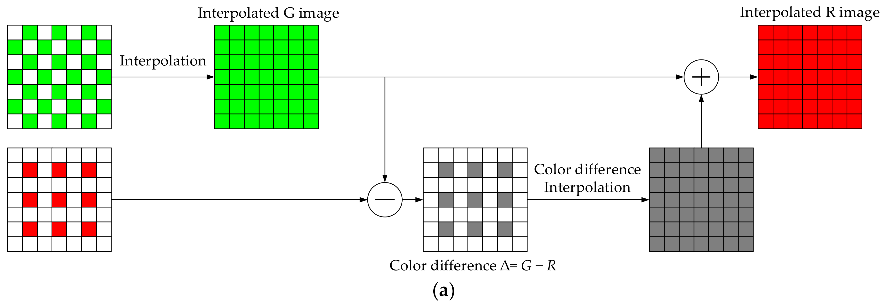
It is known that color difference interpolation and residual interpolation are common methods in the interpolation of the R/B plane. These two interpolations in the R plane are shown in Figure 2. The interpolation of B plane is the same. The first method is the color difference interpolation (CDI) [12], as shown in Figure 2a. Firstly, color difference images are produced by subtracting the interpolated G pixel values from the sample of R pixels. Then, the color difference images can be interpolated. Finally, to generate the full R images, the interpolated G pixel images are added to the interpolated color difference images.
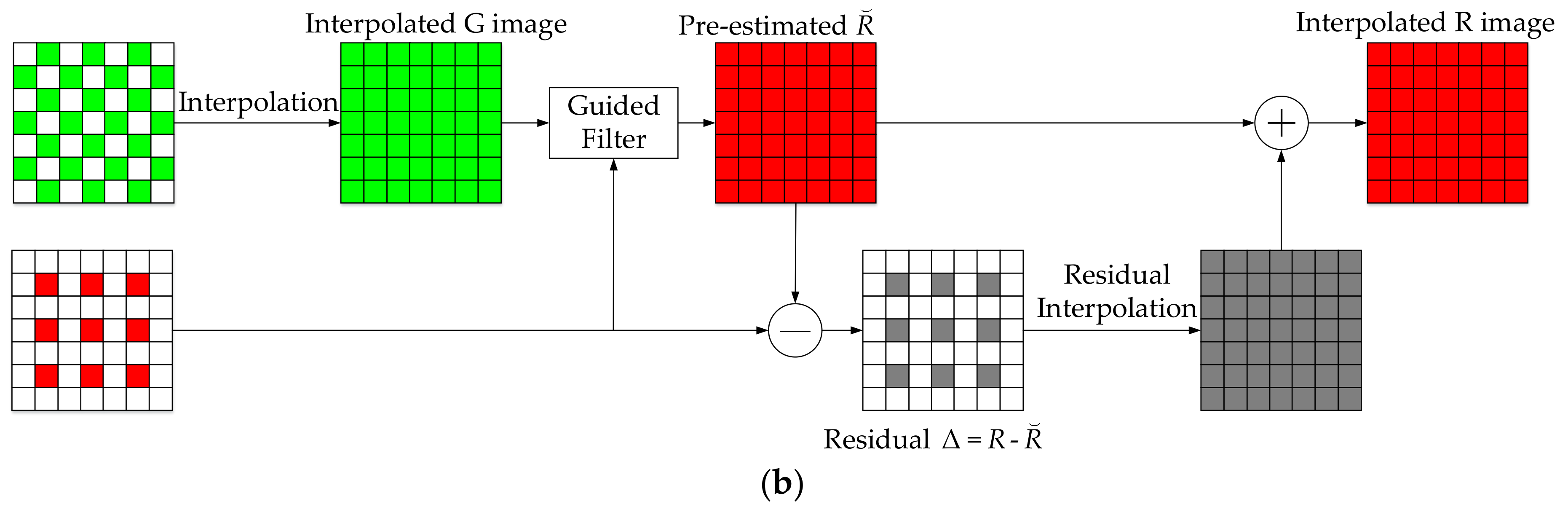
Figure 2b shows the RI [10] process of the R plane. The part that is different from CDI [12] is the estimations of R pixel values. Firstly, to get the full G images, the subsampled G components are interpolated. Secondly, the pre-estimated R pixel values () are obtained by using full G images as the guide filter for sampled R components. By subtracting the from sampled R pixels (), the residual values are obtained. Finally, to approach the interpolated image of R, the residual values are interpolated. The full R image is resumed by combining the interpolated residual image and .
2.1.2. Laplacian Energy
In Figure 2b, guide filter is used to generate the tentative image. The Laplacian energy is applied to calculate the parameters in guide filter. Therefore, before knowing the guide filter, Laplacian energy are introduced. The Laplacian energy is the quota used to represent the smoothness of images. The map of an image is calculated as:
where is the Laplacian map, is an image, and is a convolution operation. The Laplacian energy of the image is calculated as:
where is the Laplacian energy, the are the image pixel coordinates, is a set of pixel coordinates of the whole image, is the approximate Laplacian map at subsampled pixel and represents the number of whole image pixels. In [12], it indicates that the interpolated performance is better in a domain where the Laplacian energy is smaller.
However, in the realistic demosaicking process, the accurate Laplacian energy cannot be computed from the subsampled images. Therefore, an approximate Laplacian energy is used to process sampling images. The approximate Laplacian map is:
Therefore, the approximate Laplacian energy of images can be defined as:
where represents the subsampled pixel indexes and is the number of subsampled pixels.
2.1.3. The Guide Filter in MLRI
RI [10] is applied to the interpolation of R/B pixels in MLRI [12] in which the guide filter is the key point. The guide filter is a linear variable process. This process takes an input image as a guide image, which enables the output image to have edge-preserving capability. After interpolating the G pixel values, the full G image, the guide filter, which is shown in Figure 2b in a linear relation, and the minimum Laplacian energy are applied to obtain the tentative R/B pixel values in MLRI [12].
In [12], it takes the interpolation of R pixels as an example. The method for the B pixel values is done in the same manner. Since the guide image and the tentative R image have the relationship as Equation (5), when the guide image has the edge-preserving capability, the tentative R image also has the edge-preserving capability. The local window is a 5 × 5 window which centers at pixel :
where is the estimated R values at the pixel , and and are linear coefficients in the . Furthermore, from the Laplacian energy, it is known that smaller energy performs better in the image interpolation. The minimum value of is obtained from Equation (6):
where is the mask which is one for the sampled R pixels and zero for the others at the pixel , is the R values at the pixel , and is the number of pixels in . In the same way, after obtaining minimum , is calculated as:
After knowing the estimated R pixel values, according to the RI [10], the sampled R pixels are subtracted from the estimated pixel values in MLRI [12] to obtain the residual image. To obtain the interpolated image, the residual image is bilinearly interpolated. The sum of the sampled R images and the interpolated R image gives the final full R picture.
2.2. The Outline of G Interpolation in GBTF and MDWI-GF
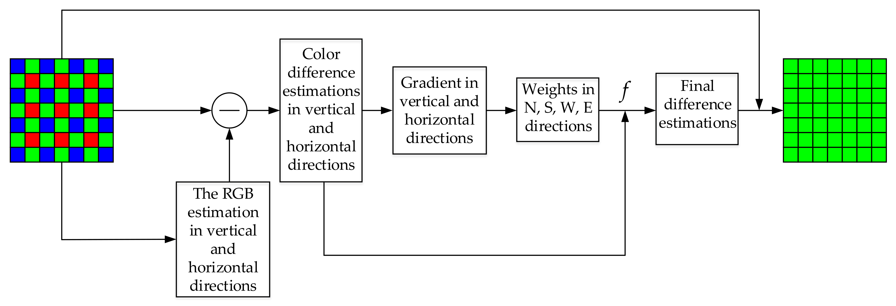
In [8], the process of interpolation of the G pixels is shown in Figure 3. The interpolated steps are roughly shown as follows.
Firstly, to obtain the G and R/B estimated pixel values in the horizontal and vertical directions, the G and R/B channel information is used.
Then, by using the estimated pixel values and the color information in the Bayer image, the horizontal and vertical color difference values are obtained. The color difference gradient values can be calculated from the color difference values. Furthermore, in the 5 × 5 window, the reciprocal of the sum of gradient of color difference in the horizontal and vertical directions is regarded as the weights in north (N), south (S), west (W), and east (E) directions.
The final estimated difference values are derived by combining the weights, the vector , and the color difference information. The G pixel value is calculated by using the final estimated difference and the R/B pixel values.
Firstly, the estimated values of G pixels in eight directions are obtained. The estimated values in W, E, N, and S directions are incorporated with the value of the G and R/B in the Bayer image. The values in the northwest (NW), northeast (NE), southwest (SW), and southeast (SE) directions are calculated by the diagonal information of G pixels passing through a filter.
Furthermore, the gradient in the eight directions is acquired from the gradient information of R, G, and B in eight directions. The weights in the eight directions is the reciprocal of the gradient.
Finally, the G pixel values can be obtained by combining the weights and values of the estimations.
3. The Proposed Algorithm
3.1. The Outline of Proposed Algorithm
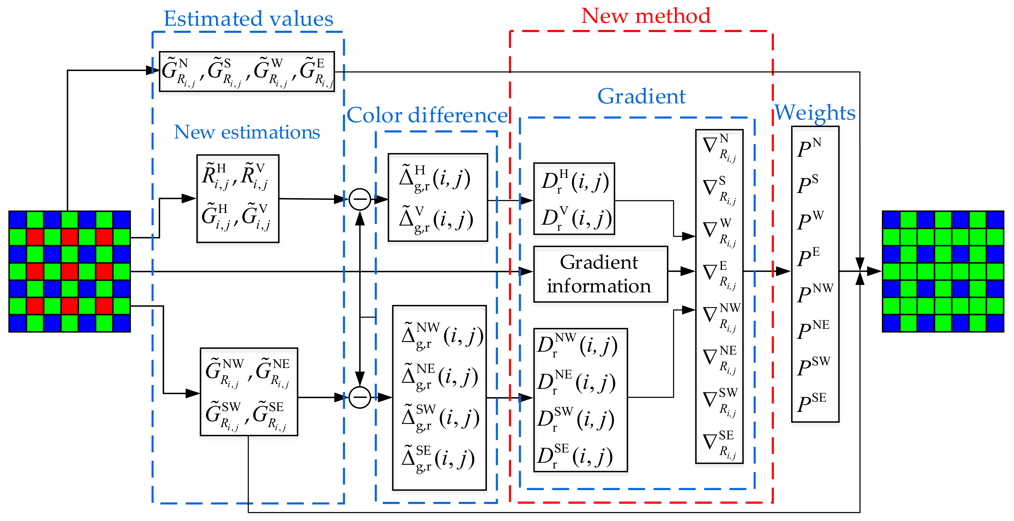
In this section, the process of the proposed algorithm is introduced. The interpolation of G pixels at R pixels is shown in Figure 5. The interpolation of G pixels at B pixels is the same. It is clear that the novel algorithm is based on the work in [8,17], shown in Figure 3, Figure 4 and Figure 5. In [17], it first obtains the estimated values in eight directions and obtains the weights of eight directions by gradient information. Then, the G pixel value is calculated. In [8], the horizontal and vertical color difference are calculated. The reciprocal of the gradient of color difference is used as the weights, and the final color difference estimations are obtained by the information of the color difference and weight information in four directions. Finally, the G pixel value is calculated by adding the R or B pixels to the final color difference estimations.
In the proposed algorithm, firstly, the first estimations of G pixels are obtained in eight directions. The color difference in the directions of NW, NE, SW, and SE is derived from the first estimated G values and R/B pixel values.
Secondly, a new method is applied to obtain the new estimated values in N, S, W, and E directions. The color difference of N, S, W, and E directions is then derived from the new estimated values. That is different from the way in [17]. At the same time, the gradient of the color difference in eight directions is calculated.
Finally, the gradient information of the color difference in eight directions and the gradient information of some parts of the RGB image are used to calculate the weights of eight directions. Those are calculated in different ways from [8]. They are also shown in Figure 5 with a red dotted line. The G pixel values are obtained from the eight-directional weights and first estimated G values. Therefore, the proposed algorithm has made great innovations on the basis of [8,17].
The full G images are utilized as the guide diagrams and the linear relation is applied in the guide filter to get the tentative estimated R values. The interpolation of R/B is the same as MLRI [12].
3.2. The Interpolation of G Values
Taking the demosaicking of G components in the R pixel of the Bayer image for example to present the process of the interpolation for G values clearly, the algorithm in B components is the same. The interpolation of eight directions will result in more effective interpolation. Therefore, the interpolation of G pixels is calculated as:
where represents eight directions, is the full G values at R pixels, is the estimations of G values in eight directions at R pixels, is the weights values in eight directions.
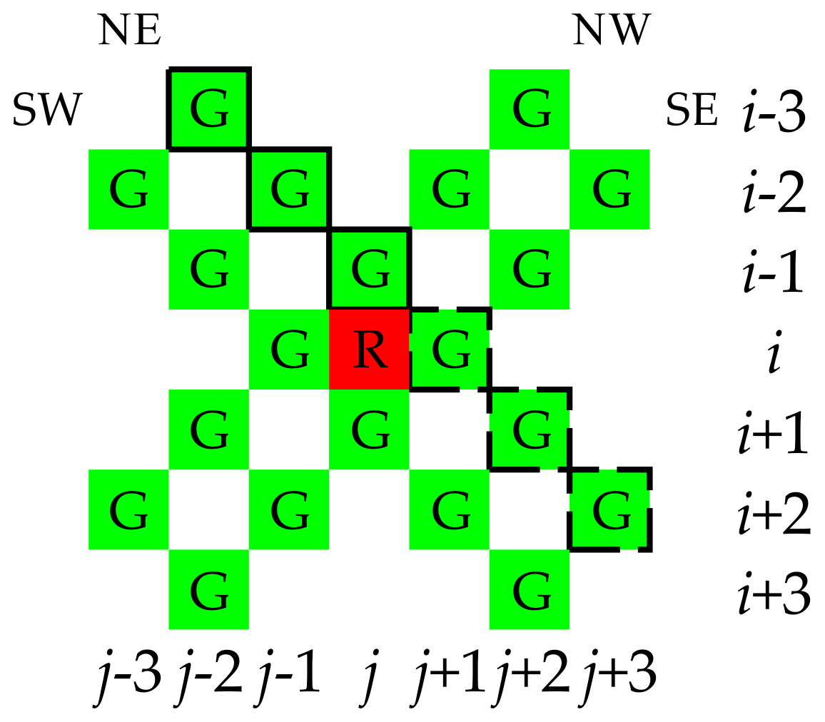
The estimations of the G pixel in the R pixel are to be conducted. In the diagonal lines, the G pixels center on the R pixel, which is shown in Figure 6. To enhance the accuracy of estimations, the estimated pixel values of G in NW, NE, SW, and SE directions in the R pixel are:
where represents the four directions (i.e., NW, NE, SW, and SE), stands for the useful information in the interpolation of G pixels in NW, NE, SW, and SE directions, is an interpolation filter.
As can be seen from Figure 6, G pixels are distributed in diagonal lines in a 7 × 7 pattern. in the NE direction is calculated by Equation (10). The other three directions (NW, SW, and SE) are similarly calculated. The position of the pixels which are used to formulate is marked by the dashed line and solid line in Figure 6.
The interpolation filter is defined as Equation (11):
The estimations of G values in N, S, W, and E directions are computed as follows:
where , , , and are the estimated G pixel values in N, S, W, and E directions in R pixels at the pixel , respectively.
After calculating the estimations of N, S, W, E, NW, NE, SW, and SE directions, are obtained in N, S, W, E, NW, NE, SW, and SE directions. is the gradient information in eight directions in R pixels at the pixel .
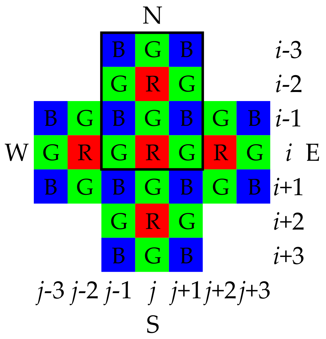
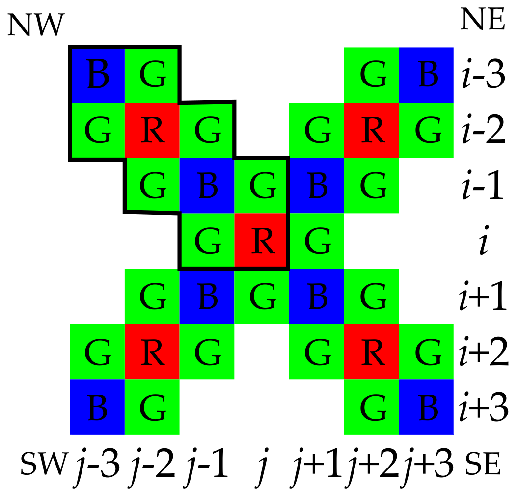
The Bayer image which takes the R pixel as the center pixel is shown in Figure 1. This image is divided into two parts to represent the gradient information. One part shown in Figure 7 contains the gradient information of R, G, and B components in N, S, W, and E directions. The other part shown in Figure 8 has the gradient information of R, G, and B components in the NW, NE, SW, and SE directions.
The gradient values of G in NW, NE, SW, and SE directions are calculated. The gradient contains the information of the gradient of the color difference and the gradient of R, G, and B values in the Bayer image. Taking the N direction shown in Figure 7 for illustration, the gradient of S, W, and E directions is calculated in the same way. Pixels used in the N direction in the Bayer image are marked with black solid lines. is defined as the gradient information in the N direction in the R pixel at the pixel . Then the gradient is defined as:
where is the gradient of color difference in vertical direction for R pixels at the pixel . In the NW direction, pixels which are used to calculate are marked with black solid lines in Figure 8. The gradient of NW direction is defined as:
where are the coordinates, is the gradient information in NW direction in R pixels at the pixel and represents the gradient of color difference in the NW direction in R pixels at the pixel . The methods in the NE, SW, and SE directions are the same as the NW direction.
The gradient of color difference in the NW direction is obtained as:
where is the color difference in the NW direction between estimated G values and R image at the pixel . The gradient of color difference in NE, SW, and SE is calculated in a similar way.
According to the estimations in the four diagonal directions, the color difference is calculated in R position. Taking the NW direction for example, the color difference of other three directions (NE, SW, and SE) at the pixel are calculated in the same way. The color difference in NW direction is defined as:
After that, the gradient of the color difference is obtained in the horizontal and vertical directions, respectively:
where is the gradient of the color difference in the horizontal direction in R pixels at the pixel , is the gradient of the color difference in the vertical direction in R pixels at the pixel , represents the color difference in the horizontal direction between the new estimated G values and R image or between G image and new estimated R values at the pixel , and is the color difference in the vertical direction between the new estimated G values and R image or between G image and the new estimated R values at the pixel .
The color difference in the horizontal and vertical directions is shown in Equations (19) and (20):
where and are the new estimated G values in the horizontal and vertical directions in the pixel , respectively, and and are the new estimated R values in the horizontal and vertical directions in the pixel , respectively.
In the horizontal and vertical directions, however, the new estimations of G pixel values and R pixel values in the pixel are shown in Equation (21), which is different from the method used in the first estimations. The new estimations are formulated as:
4. Experimental Results and Discussions
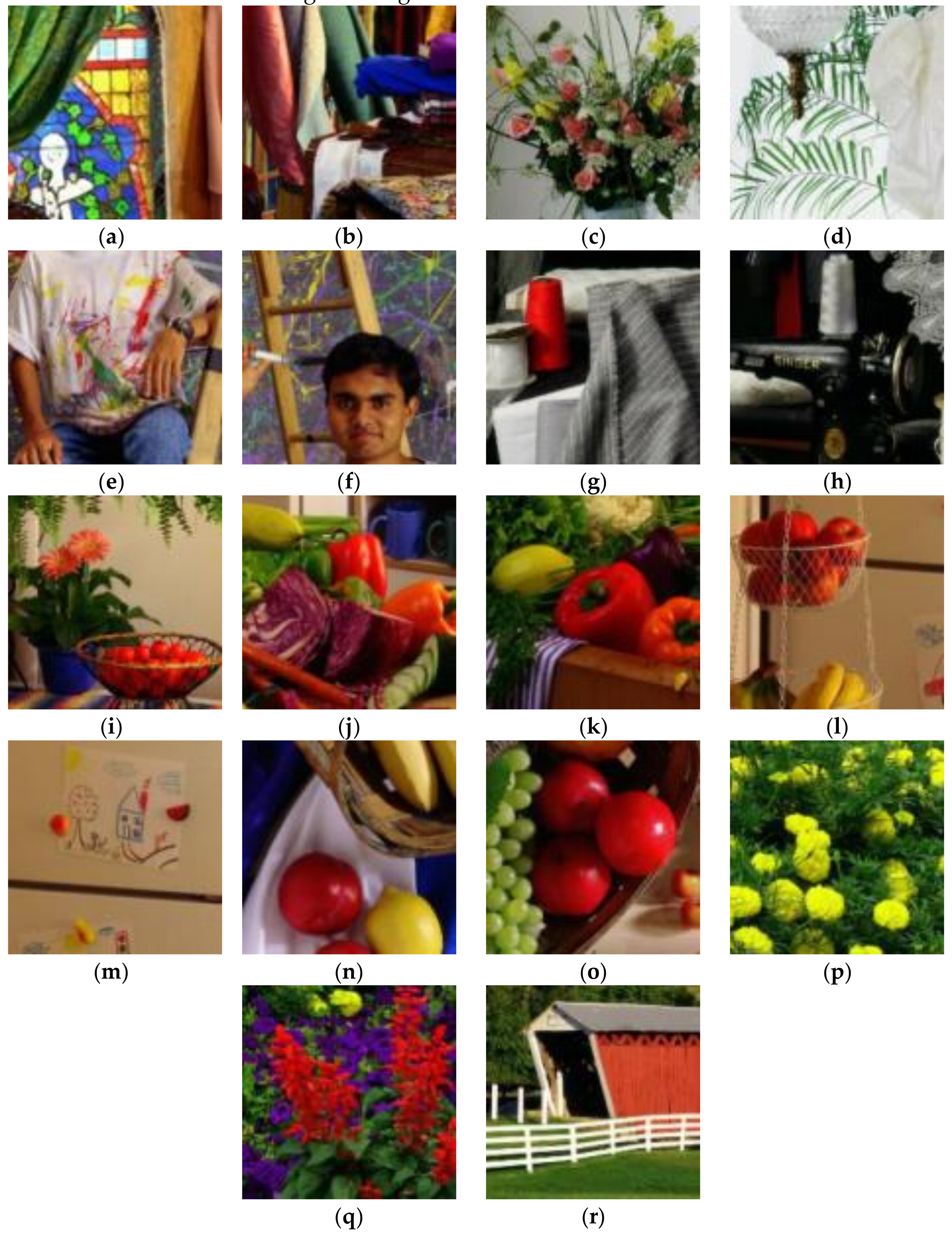
In order to know the interpolated effect of the proposed method, we carried out the experiment by using MATLAB R2015a with an Intel(R) Core(TM), i5-5200U 2.20 GHz CPU, 4.00 GB memory computer. The sampled data of the McMaster (McM) images shown in Figure 9 is used for testing. The original sequence of Bayer is B, G, G, R. To demonstrate the effect of the proposed method, the experimental results are compared with DLMMSE [2], IG [6], GBTF [8], RI [10], MLRI [12], and MDWI-GF [17].
The peak signal-to-noise ratio (PSNR) is widely used in the estimate. The results are shown in Table 1. Two decimal digits are retained. In each image, the best processing result has been marked in black bold font. In Table 1, the PSNR in the average values of images which are processed by MLRI [12] is the maximum value and the proposed algorithm is the secondary one. However, in Figure 9a,e,f,h,i,j,l,m,n,o,q, the PSNR of the proposed algorithm is higher than that of MLRI [12]. The proposed algorithm does not obtain the best result in all images. It performs best in Figure 9a,e,f,i,m,o,q. Especially in Figure 9f, the proposed algorithm (EWGCD) improves significantly, reaching 5.65 dB higher than GBTF [8]. However, EWGCD does not make a greater promotion in Figure 9c,g.
The structural similarity (SSIM) index measurement works well in measuring the similarity of the interpolated image to the original one. The results are listed in Table 2. Four decimal digits are retained. The maximum average value of the SSIM for all images has been marked in black bold font. From Table 2, the average values of SSIM show that the image which is interpolated by the proposed method is more similar to the original image.
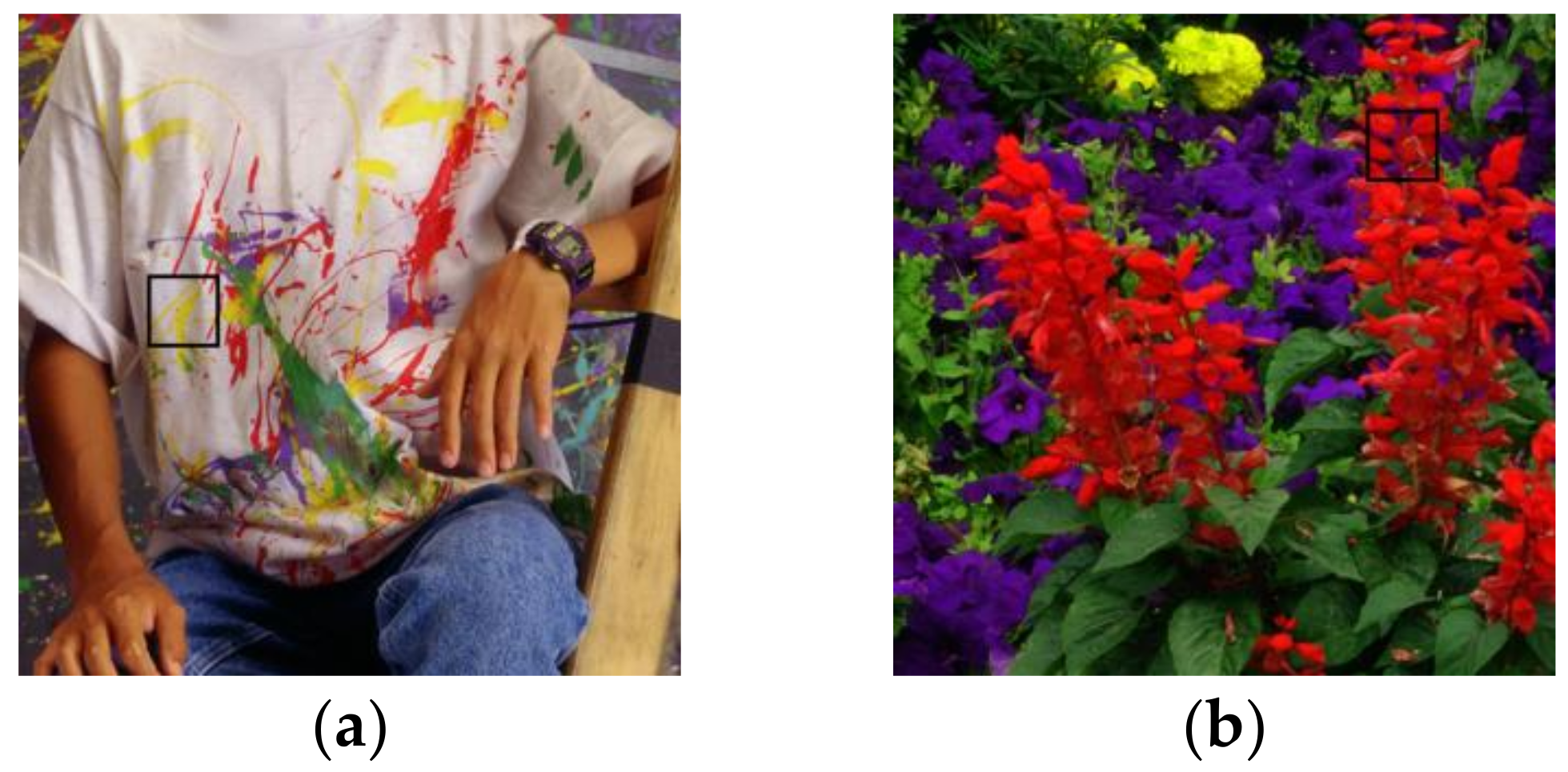
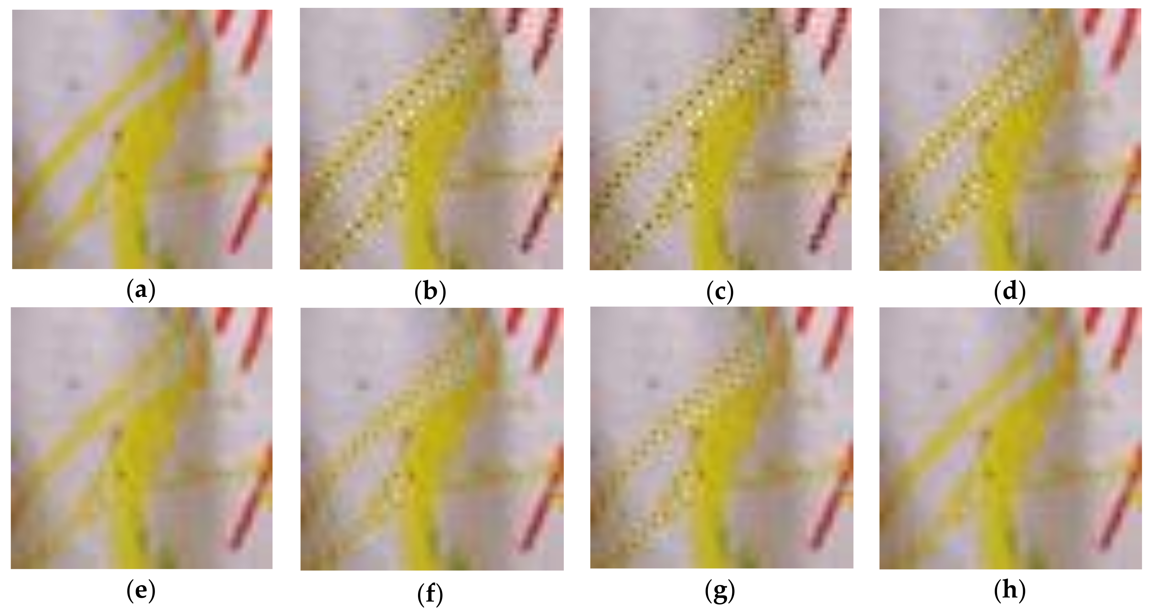
Furthermore, two images are shown in Figure 10 to see the effect of the proposed algorithm in the local magnification. The two images are Figure 9e,q. The local part of Figure 9e is magnified. The magnified part, which is marked by a black box, is shown in Figure 10a. The magnified local images, which have a visual comparison, are shown in Figure 11. The magnified image can be clearly seen in Figure 11a. The other seven images, which are magnified in the same part as shown in Figure 11, are obtained by DLMMSE [2], IG [6], GBTF [8], RI [10], MLRI [12], MDWI-GF [17], and the proposed method, respectively. Compared with the other six methods, the proposed one is visually more similar to the original one. Visual distortions are present, as can be seen in Figure 11, where the yellow part has grey spots from Figure 11b–g. Compared with the original image shown in Figure 11a, the distortion from Figure 11b–e is particularly serious. Though the image which is processed by the proposed algorithm has a little blur at the edge of yellow part, it has a better performance than the other six algorithms.
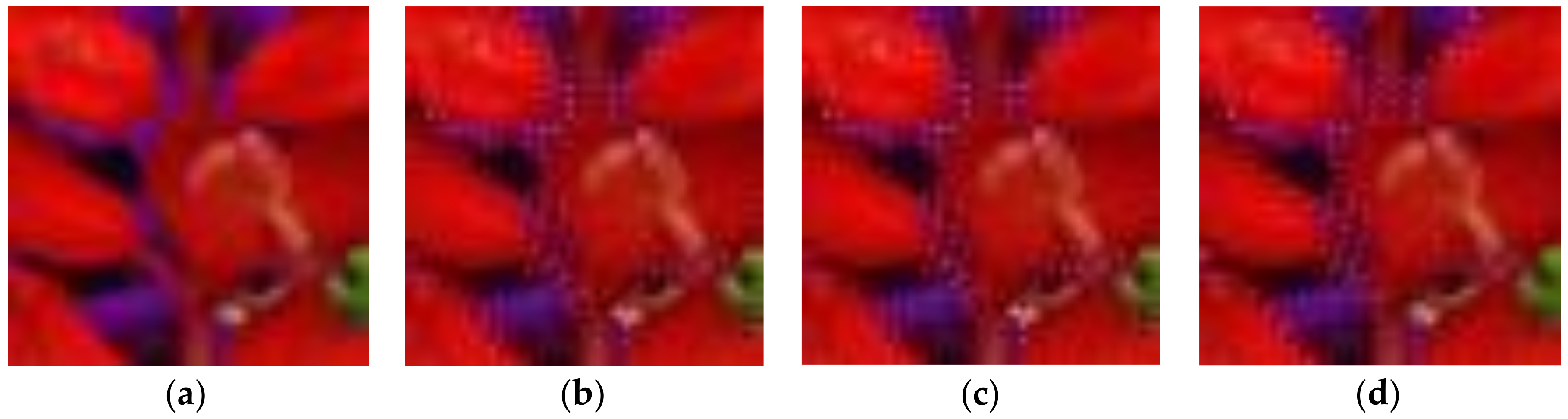
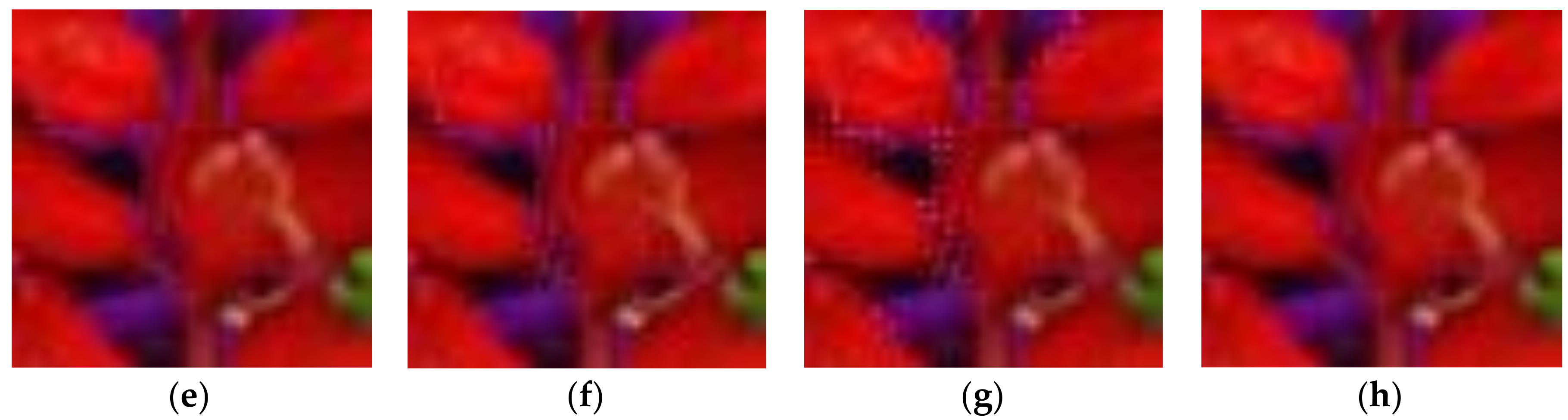
The local part of Figure 9q, which is marked by a black box in Figure 10b, is magnified as well. There are eight magnified images shown in Figure 12. The magnified part of the original image is shown in Figure 12a. The other seven images in Figure 12 are the same magnified part as the original one by DLMMSE [2], IG [6], GBTF [8], RI [10], MLRI [12], MDWI-GF [17], and the proposed method, respectively. It can be seen that slightly white granular spots which are the distortion appear in the purple parts from Figure 12b–e. Though the proposed algorithm has distortions at the edge of the purple parts, as shown in Figure 12h, the distortion is more serious, visually, as shown in Figure 12b–g.
5. Conclusions
In this paper, a new algorithm is proposed in demosaicking by eight-directional weights based on the gradient of the color difference for the Bayer image. We first interpolate G pixels by considering the weights and estimated G values in the eight directions. Then, a filter and the diagonal G values are utilized to obtain the estimated G values in NW, NE, SW, and SE directions. The estimated G values in N, S, W, and E directions are calculated by pixel values in the Bayer image. These estimated values in NW, NE, SW, and SE are applied to the color difference, while in N, S, W, and E directions, the estimated values used to obtain the color difference are calculated in a new method. The gradient of the color difference is obtained in eight directions. This gradient is used to calculate the weights in eight directions. The weights and first estimated G are applied to generate the full G image. The interpolation of R/B values is the same as MLRI. Compared with the other six algorithms, the experimental results demonstrate that our proposed method has different degrees of improvement in the results of eighteen McM images objectively and subjectively. In our future work, we will concentrate on the improvement of the interpolation of R/B pixels and the operating efficiency of demosaicking in G pixels.
Author Contributions
Y.L., C.W., and H.Z. conceived the algorithm and designed the experiments; Y.L., H.Z., and J.S. performed the experiments; Y.L. and C.W. analyzed the results; Y.L. drafted the manuscript; and Y.L., C.W., H.Z., J.S., and S.C. revised the manuscript. All authors read and approved the final manuscript.
Acknowledgments
This work was supported by the National Natural Science Foundation of China (no. 61702303), the Shandong Provincial Natural Science Foundation, China (no. ZR2017MF020), and the 12th Student Research Training Program (SRTP) at Shandong University (Weihai), China.
Conflicts of Interest
The authors declare no conflict of interest.
References
- Wang, D.Y.; Yu, G.; Zhou, X.; Wang, C.Y. Image Demosaicking for Bayer-Patterned CFA Images Using Improved Linear Interpolation. In Proceedings of the 7th International Conference on Information Science and Technology, Da Nang, Vietnam, 16–19 April 2017; pp. 464–469. [Google Scholar]
- Zhang, L.; Wu, X. Color demosaicking via directional linear minimum mean square-error estimation. IEEE Trans. Image Process. 2005, 14, 2167–2178. [Google Scholar] [CrossRef] [PubMed] [Green Version]
- Zhang, L.; Wu, X.; Buades, A.; Li, X. Color demosaicking by local directional interpolation and nonlocal adaptive thresholding. J. Electron. Imaging 2011, 20, 16. [Google Scholar]
- Wu, J.; Anisetti, M.; Wu, W.; Damiani, E.; Jeon, G. Bayer demosaicking with polynomial interpolation. IEEE Trans. Image Process. 2016, 25, 5369–5382. [Google Scholar] [CrossRef] [PubMed]
- Chen, W.-J.; Chang, P.-Y. Effective demosaicking algorithm based on edge property for color filter arrays. Digit. Signal Process. 2012, 22, 163–169. [Google Scholar] [CrossRef]
- Chung, K.-H.; Chan, Y.-H. Low-complexity color demosaicing algorithm based on integrated gradients. J. Electron. Imaging 2010, 19, 15. [Google Scholar] [CrossRef] [Green Version]
- Pekkucuksen, I.; Altunbasak, Y. Edge strength filter based color filter array interpolation. IEEE Trans. Image Process. 2012, 21, 393–397. [Google Scholar] [CrossRef] [PubMed]
- Pekkucuksen, I.; Altunbasak, Y. Gradient Based Threshold Free Color Filter Array Interpolation. In Proceedings of the IEEE International Conference on Image Processing, Hong Kong, China, 26–29 September 2010; pp. 137–140. [Google Scholar]
- Wang, J.; Wu, J.; Wu, Z.; Jeon, G. Filter-based Bayer pattern CFA demosaicking. Circuits Syst. Signal Process. 2017, 36, 2917–2940. [Google Scholar] [CrossRef]
- Kiku, D.; Monno, Y.; Tanaka, M.; Okutomi, M. Residual interpolation for color image demosaicking. IEEE Tokyo Inst. Technol. 2013, 978, 2304–2308. [Google Scholar]
- He, K.; Sun, J.; Tang, X. Guided image filtering. IEEE Trans. Pattern Anal. Mach. Intell. 2013, 35, 1397–1409. [Google Scholar] [CrossRef] [PubMed]
- Kiku, D.; Monno, Y.; Tanaka, M.; Okutomi, M. Minimized-Laplacian Residual Interpolation for Color Image Demosaicking. In Proceedings of the SPIE, Digital Photography X, San Francisco, CA, USA, 3–5 February 2014; Volume 9023, pp. 1–8. [Google Scholar]
- Kiku, D.; Monno, Y.; Tanaka, M.; Okutomi, M. Beyond color difference: Residual interpolation for color image demosaicking. IEEE Trans. Image Process. 2016, 25, 1288–1300. [Google Scholar] [CrossRef] [PubMed]
- Ye, W.; Ma, K.K. Color image demosaicking using iterative residual interpolation. IEEE Trans. Image Process. 2015, 24, 5879–5891. [Google Scholar] [CrossRef] [PubMed]
- Kim, Y.; Jeong, J. Four-direction residual interpolation for demosaicking. IEEE Trans. Circuits Syst. Video Technol. 2016, 26, 881–890. [Google Scholar] [CrossRef]
- Monno, Y.; Kiku, D.; Tanaka, M.; Okutomi, M. Adaptive residual interpolation for color and multispectral image demosaicking. Sensors 2017, 17, 21. [Google Scholar] [CrossRef] [PubMed]
- Wang, L.; Jeon, G. Bayer pattern CFA demosaicking based on multi-directional weighted interpolation and guided filter. IEEE Signal Process. Lett. 2015, 22, 2083–2087. [Google Scholar] [CrossRef]
- Satya Prakash, V.N.V.; Satya Prasad, K.; Jaya Chandra Prasad, T. Demosaicing of color images by accurate estimation of luminance. Telkomnika 2016, 14, 47–55. [Google Scholar] [CrossRef]
- Ji, Y.K.; Sang, W.P.; Min, K.P.; Kang, M.G. Aliasing artifacts reduction with subband signal analysis for demosaicked images. Digit. Signal Process. 2016, 59, 115–128. [Google Scholar]
- Wu, J.; Timofte, R.; Gool, L.V. Demosaicing based on directional difference regression and efficient regression priors. IEEE Trans. Image Process. 2016, 25, 3862–3874. [Google Scholar] [CrossRef] [PubMed]
- Yang, B.; Luo, J.; Guo, L.; Cheng, F. Simultaneous image fusion and demosaicing via compressive sensing. Inf. Process. Lett. 2016, 116, 447–454. [Google Scholar] [CrossRef]
Figure 1.
Color filter array (Bayer pattern).

Figure 2.
The process of interpolation in the R plane: (a) the process of color difference interpolation (CDI) [12] and (b) the process of residual interpolation (RI) [10].


Figure 3.
The process of G interpolation in GBTF [8].
Figure 3.
The process of G interpolation in GBTF [8].

Figure 4.
The process of G interpolation in MDWI-GF [17].
Figure 4.
The process of G interpolation in MDWI-GF [17].

Figure 5.
The process of G interpolation in the proposed algorithm in R pixels.

Figure 6.
The G pixels in four diagonals.

Figure 7.
The gradient information of N, S, W, and E directions.

Figure 8.
The gradient information of NW, NE, SW, and SE directions.

Figure 9.
The McM images used to simulate.

Figure 10.
The images used to magnify the local part: (a) the text image Figure 9e and (b) the test image Figure 9q.

Figure 11.
Subjective quality comparison of the partial Figure 9e: (a) original, (b) DLMMSE [2], (c) IG [6], (d) GBTF [8], (e) RI [10], (f) MLRI [12], (g) MDWI-GF [17], and (h) the proposed method.

Figure 12.
Subjective quality comparison of partial Figure 9q: (a) original, (b) DLMMSE [2], (c) IG [6], (d) GBTF [8], (e) RI [10], (f) MLRI [12], (g) MDWI-GF [17], and (h) the proposed method.


Table 1.
PSNR (dB) of the proposed method compared with DLMMSE [2], IG [6], GBTF [8], RI [10], MLRI [12], and MDWI-GF [17].
| Test Images | DLMMSE [2] | IG [6] | GBTF [8] | RI [10] | MLRI [12] | MDWI-GF [17] | Proposed |
|---|---|---|---|---|---|---|---|
| Figure 9a | 26.98 | 28.52 | 26.89 | 28.89 | 28.98 | 29.23 | 29.36 |
| Figure 9b | 33.69 | 34.62 | 33.62 | 34.83 | 35.06 | 34.80 | 34.83 |
| Figure 9c | 32.59 | 32.63 | 32.69 | 33.80 | 33.85 | 32.58 | 32.48 |
| Figure 9d | 34.33 | 34.89 | 34.74 | 37.53 | 37.66 | 37.26 | 37.20 |
| Figure 9e | 31.28 | 33.25 | 30.92 | 33.47 | 33.94 | 34.25 | 34.41 |
| Figure 9f | 33.83 | 37.11 | 33.21 | 37.73 | 38.29 | 38.83 | 38.86 |
| Figure 9g | 38.65 | 36.80 | 38.97 | 37.62 | 37.50 | 35.31 | 35.18 |
| Figure 9h | 37.46 | 36.72 | 37.50 | 36.03 | 37.05 | 35.62 | 37.06 |
| Figure 9i | 34.41 | 35.48 | 34.31 | 35.71 | 36.49 | 36.62 | 37.10 |
| Figure 9j | 36.34 | 37.90 | 36.25 | 37.92 | 38.65 | 38.77 | 38.75 |
| Figure 9k | 37.24 | 39.30 | 37.04 | 39.40 | 39.98 | 39.99 | 39.85 |
| Figure 9l | 36.61 | 38.86 | 36.65 | 39.53 | 39.65 | 38.21 | 38.32 |
| Figure 9m | 38.80 | 40.10 | 38.65 | 40.07 | 40.63 | 40.56 | 40.61 |
| Figure 9n | 37.24 | 38.30 | 37.10 | 38.72 | 38.81 | 38.96 | 38.87 |
| Figure 9o | 37.27 | 38.35 | 37.09 | 38.17 | 38.92 | 39.12 | 39.15 |
| Figure 9p | 30.45 | 34.54 | 30.08 | 34.90 | 35.16 | 35.21 | 34.99 |
| Figure 9q | 29.31 | 31.07 | 29.02 | 31.77 | 32.58 | 33.15 | 33.48 |
| Figure 9r | 33.90 | 35.49 | 34.04 | 36.48 | 36.12 | 35.54 | 35.57 |
| Average | 34.47 | 35.77 | 34.38 | 36.25 | 36.63 | 36.33 | 36.45 |
Table 2.
SSIM of the proposed method compared with DLMMSE [2], IG [6], GBTF [8], RI [10], MLRI [12], and MDWI-GF [17].
| Test Images | DLMMSE [2] | IG [6] | GBTF [8] | RI [10] | MLRI [12] | MDWI-GF [17] | Proposed |
|---|---|---|---|---|---|---|---|
| Figure 9a | 0.9791 | 0.9882 | 0.9852 | 0.9891 | 0.9899 | 0.9905 | 0.9910 |
| Figure 9b | 0.9910 | 0.9958 | 0.9962 | 0.9970 | 0.9969 | 0.9968 | 0.9970 |
| Figure 9c | 0.9945 | 0.9944 | 0.9951 | 0.9967 | 0.9962 | 0.9966 | 0.9965 |
| Figure 9d | 0.9958 | 0.9968 | 0.9967 | 0.9990 | 0.9984 | 0.9988 | 0.9987 |
| Figure 9e | 0.9937 | 0.9964 | 0.9957 | 0.9975 | 0.9976 | 0.9977 | 0.9979 |
| Figure 9f | 0.9895 | 0.9954 | 0.9939 | 0.9963 | 0.9968 | 0.9969 | 0.9971 |
| Figure 9g | 0.9990 | 0.9981 | 0.9990 | 0.9986 | 0.9988 | 0.9987 | 0.9985 |
| Figure 9h | 0.9980 | 0.9957 | 0.9976 | 0.9972 | 0.9980 | 0.9980 | 0.9976 |
| Figure 9i | 0.9939 | 0.9965 | 0.9966 | 0.9979 | 0.9978 | 0.9979 | 0.9982 |
| Figure 9j | 0.9883 | 0.9970 | 0.9968 | 0.9981 | 0.9980 | 0.9981 | 0.9984 |
| Figure 9k | 0.9886 | 0.9965 | 0.9971 | 0.9979 | 0.9979 | 0.9978 | 0.9982 |
| Figure 9l | 0.9907 | 0.9983 | 0.9997 | 0.9990 | 0.9990 | 0.9993 | 0.9996 |
| Figure 9m | 0.9941 | 0.9989 | 0.9991 | 0.9994 | 0.9993 | 0.9992 | 0.9994 |
| Figure 9n | 0.9886 | 0.9979 | 0.9980 | 0.9986 | 0.9987 | 0.9984 | 0.9988 |
| Figure 9o | 0.9906 | 0.9974 | 0.9980 | 0.9982 | 0.9986 | 0.9983 | 0.9987 |
| Figure 9p | 0.9821 | 0.9940 | 0.9918 | 0.9956 | 0.9956 | 0.9959 | 0.9964 |
| Figure 9q | 0.9691 | 0.9784 | 0.9818 | 0.9874 | 0.9879 | 0.9885 | 0.9898 |
| Figure 9r | 0.9925 | 0.9968 | 0.9970 | 0.9982 | 0.9979 | 0.9977 | 0.9977 |
| Average | 0.9899 | 0.9951 | 0.9953 | 0.9968 | 0.9968 | 0.9970 | 0.9972 |
© 2018 by the authors. Licensee MDPI, Basel, Switzerland. This article is an open access article distributed under the terms and conditions of the Creative Commons Attribution (CC BY) license (http://creativecommons.org/licenses/by/4.0/).
Share and Cite
MDPI and ACS Style
Liu, Y.; Wang, C.; Zhao, H.; Song, J.; Chen, S. Bayer Image Demosaicking Using Eight-Directional Weights Based on the Gradient of Color Difference. Symmetry 2018, 10, 222. https://doi.org/10.3390/sym10060222
AMA Style
Liu Y, Wang C, Zhao H, Song J, Chen S. Bayer Image Demosaicking Using Eight-Directional Weights Based on the Gradient of Color Difference. Symmetry. 2018; 10(6):222. https://doi.org/10.3390/sym10060222
Chicago/Turabian StyleLiu, Yizheng, Chengyou Wang, Hongming Zhao, Jiayang Song, and Shiyue Chen. 2018. "Bayer Image Demosaicking Using Eight-Directional Weights Based on the Gradient of Color Difference" Symmetry 10, no. 6: 222. https://doi.org/10.3390/sym10060222
Note that from the first issue of 2016, this journal uses article numbers instead of page numbers. See further details here.