A Bi-Level Programming Model for the Railway Express Cargo Service Network Design Problem

Abstract

Service network design is fundamentally crucial for railway express cargo transportation. The main challenge is to strike a balance between two conflicting objectives: low network setup costs and high expected operational incomes. Different configurations of these objectives will have different impacts on the quality of freight transportation services. In this paper, a bi-level programming model for the railway express cargo service network design problem is proposed. The upper-level model forms the optimal decisions in terms of the service characteristics, and the low-level model selects the service arcs for each commodity. The rail express cargo is strictly subject to the service commitment, the capacity restriction, flow balance constraints, and logical relationship constraints among the decisions variables. Moreover, linearization techniques are used to convert the lower-level model to a linear one so that it can be directly solved by a standard optimization solver. Finally, a real-world case study based on the Beijing–Guangzhou Railway Line is carried out to demonstrate the effectiveness and efficiency of the proposed solution approach.

1. Introduction

In recent years, the competition between railway and highway transportation has become increasingly intense, especially for the long-distance transportation of high-value freight. The governments expect that more freight flow transported by highways should be diverted to the railways in order to reduce carbon emissions. For example, in Europe, 30% of road freight over 300 km is expected to shift to railways or waterways by 2030. The Ministry of Transport of China also recommends that the railways and waterways should support more freight transportation [1]. However, road freight transport is convenient and efficient currently, and many shippers tend to choose the road transportation mode. Therefore, as one of the largest and busiest railway systems, the China Railway has focused on the development of scheduled train services during past years in an effort to obtain a higher market share in the high-value freight transportation. Among them, the Railway Express Cargo Service Network Design problem (RECSNDP) is the key issue that needs to be addressed in both theory and practice.

The RECSNDP requires the determination of the train operation plans and a set of shipment delivery strategies on the network, which satisfies target customer demand with an acceptable level of service at minimum cost, and without violating capacity restrictions. The prominent features of it are the focus on fast transport, guaranteed pickup and delivery times for customers.

The RECSNDP is normally viewed as a tactical planning problem in which the railway company has to decide which terminals should provide with direct transportation services and at what frequency. Although closely related to classic network flow problems [2], which can be solved very efficiently, the service network design problem has been proven to be one of the most difficult combinatorial optimization problems [3]. Solving real-life problem instances to optimality is generally not possible.

2. Literature Review

The RECSNDP is usually concerned with finding a cost-minimizing transportation network configuration that satisfies the delivery requirements for the target commodities. More specifically, the RECSNDP involves searching for optimal decisions in terms of the service characteristics (for example, the selection of routes to utilize and the speed level, the stopping patterns and the service frequency), and the service arc selection for each commodity. Crainic [4] stated that service network design problems are essential in the construction of a transportation network. Their formulations are associated with the long-term evolution of transportation infrastructures and services.

There exists a rich body of literature on the RECSNDP. A classical paper is that of Crainic et al. [5], who studied the interactions between blocking, routing, and makeup for a Canadian freight system. Campetella et al. [6] considered an Italian freight service of a size comparable to that of SBB Cargo Express, for which they do did traffic routing, and service frequency and empty cars planning in an integrated manner, ignoring the train load limits and yard capacities. Ahuja et al. [7] proposed a particularly detailed model for the blocking problem arising in the United States. Ceselli et al. [8] established three models for the express service network of Swiss federal railways using different methods and designed corresponding solution methods that include commercial solver approach, branch-and-cut approach, and column generation based approach. Lin et al. [9] presented a formulation and solution for the train connection service problem in China railway network in order to determine the optimal freight train service, the frequency of service, and the distribution of classification workload among yards. Zhu et al. [10] addressed the scheduled service network design problem by proposing a model that combined service selection and scheduling, car classification and blocking, train makeup, and the routing of time-dependent customer shipments based on a cyclic three-layer space-time network representation of the associated operations and decisions and their relations and time dimensions. A methodology integrating slope scaling, a dynamic block generation mechanism, long-term memory-based perturbation strategies, and an ellipsoidal search was proposed, which is efficient and robust and yielded high-quality solutions. This literature above researched the railway service network by designing of train formation plans. Meanwhile, several studies solved the railway blocking problem as the network design problem. Newton et al. [11] modeled the railway blocking problem as a network design problem with the objective of minimizing the total mileage, handling and delay costs. They also developed a column generation, branch-and-bound algorithm to solve the model. Barnhart et al. [12] formulated the railroad blocking problem as a network design problem with maximum degree and flow constraints on the nodes and proposed a heuristic Lagrange relaxation approach to solve the problem. The model was tested on a major railroad, and the validity of the model and algorithm were verified.

Service network design also exists in other types of transportation systems and fields. Barnhart and her research team [13,14,15] addressed a real-life air cargo express delivery service network design problem. That problem is characterized by a hub-and-spoke network structure and additional complex constraints which do not exist in the general service network design problem model. A column generation based method was able to solve the problem successfully within a reasonable time. However, it may be difficult to generalize the model to other freight transportation applications, especially to those without hub-and-spoke structures. In addition, their methods cannot be used for integrated service network design when several classes of services (first class, second class, deferred class, etc.) are planned simultaneously. Yang and Chen [16] investigated a two-stage stochastic model for the air freight network design problems with uncertain demand. The top-level decision variables of this problem included the number and location of air freight hubs, while the second stage consisted of decisions of flight routes and flows. The model was tested for the air passenger data in Taiwan and mainland China. Detailed reviews of such research efforts can also be found in Christiansen et al. [17] for maritime transportation, Wang and Lo [18] for ferry service network design, Nourbakhsh and Ouyang [19] for public transit network optimization, Crainic [4] for long-haul transportation, Bai et al. [20] for stochastic service network design, Ji et al. [21] for intermodal transportation network design problem, Di et al. [22] for ridesharing network design problem, and Liu et al. [23] for boundedly rational decision rules of travelers in a dynamic transit service network.

In this paper, we propose a bi-level programming formulation for the railway express cargo service network design problem. In the upper-level model, optimal decisions in terms of the service characteristics are made, i.e., train operation plan. However, among them, the operating frequency of the scheduled trains is unknown, which is determined by the lower-level model. Meanwhile, the lower-level model carries out the flow distribution according to the train operation plan and service commitments. Note that, the rail express cargo is strictly subject to the prescribed transit time. The overall transportation time consists of two parts: the transportation time on arcs and the transfer time between arcs. The proportions of the volume of shipments that are able to be transported are also to be determined by solving the lower-level model.

The remainder of this paper is organized as follows. Section 3 describes the express cargo service network design problem in detail. Section 4 provides a bi-level model formulation and its linearized version. A numerical example is conducted in Section 5. Finally, the conclusions of this paper are presented in Section 6.

3. Problem Description

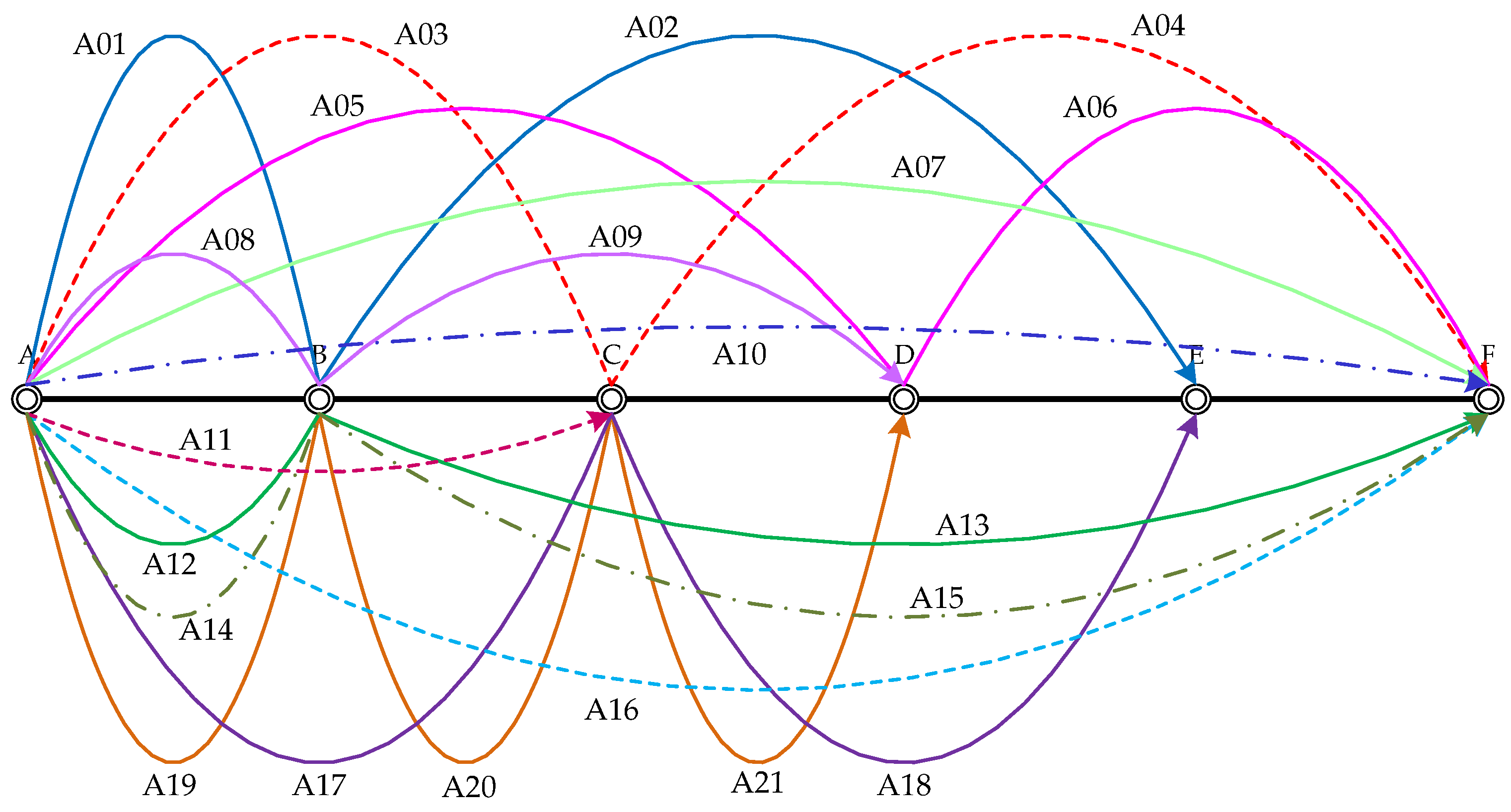
The RECSNDP, like the general service network design problem (SNDP), involves two types of decisions: the first is to determine the service network formed by the movements in space and time of the various trains and the second is to assign the shipments to the service network. The key to the formation of the service network is to split the train service into a sequence of service arcs. Since the train operation plan is unknown, we need to consider all of the potential train service arcs derived from the reasonable trains involving the origin station, the destination station, the stopping patterns, the speed levels and the service frequency. To better explain the process of generating the service network and assigning the shipments to the service network, in the following we would like to provide more details using the example depicted in Figure 1.

Figure 1 presents a simple railway network. The network contains six stations, named A~F, along the railway line. We generate a potential train operation plan according to the shipment characteristics on the railway network, which includes 12 trains that are denoted by the lines with different styles and colors (see Figure 1). Different line styles represent different levels of speed, i.e., a solid line represents 80 km/h, a dashed line represents 120 km/h, and a dot-and-dash line represents 160 km/h. In this way, a service network is constructed, which includes twenty-one service arcs. Note that all the arcs differ from each other even they belong to the same train. For example, though the service arc A01 and service arc A02 belong to the same train, they are regarded as different service arcs. Moreover, even the origin station and destination station of two arcs are the same, they may be different arcs, such as arc A01 and arc A08. In order to express the service network conveniently, we convert the trains into a matrix. In this way, each train can be described by the service network (see

Table 1. Train operation plan.

Train	Speed (km/h)	A ↓ B	A ↓ C	A ↓ D	A ↓ E	A ↓ F	B ↓ C	B ↓ D	B ↓ E	B ↓ F	C ↓ D	C ↓ E	C ↓ F	D ↓ E	D ↓ F	E ↓ F
1	80	1	0	0	0	0	0	0	1	0	0	0	0	0	0	0
2	120	0	1	0	0	0	0	0	0	0	0	0	1	0	0	0
3	80	0	0	1	0	0	0	0	0	0	0	0	0	0	1	0
4	80	0	0	0	0	1	0	0	0	0	0	0	0	0	0	0
5	80	1	0	0	0	0	0	1	0	0	0	0	0	0	0	0
6	160	0	0	0	0	1	0	0	0	0	0	0	0	0	0	0
7	120	0	1	0	0	0	0	0	0	0	0	0	0	0	0	0
8	80	1	0	0	0	0	0	0	0	1	0	0	0	0	0	0
9	160	1	0	0	0	0	0	0	0	1	0	0	0	0	0	0
10	120	0	0	0	0	1	0	0	0	0	0	0	0	0	0	0
11	80	0	1	0	0	0	0	0	0	0	0	1	0	0	0	0
12	80	1	0	0	0	0	1	0	0	0	1	0	0	0	0	0

). Meanwhile, all of the service arcs can be identified from the matrix.

In addition, the service arc can be rewritten as (the origin station, the destination station, travel time, train ID). For example, if the distance between A and B is 500 km, then the arc A→B provided by train 1 can be expressed as (A, B, 500/80, 1). In practice, there may exist a series of train operation plans that match the shipment characteristics and we can generate these plans using above mentioned method. Clearly, one plan corresponds to a service network.

The second step is to assign the shipments to the service network based on the train operation plan. For example, shipment 1: A→E is considered on the complete service network. The possible transportation strategies that can be adopted by the carrier include (but are not limited to) the following:

(1)

A$\stackrel{\mathrm{A}01}{\to }$B$\stackrel{\mathrm{A}02}{\to }$E;

(2)

A$\stackrel{\mathrm{A}17}{\to }$C$\stackrel{\mathrm{A}18}{\to }$E;

(3)

A$\stackrel{\mathrm{A}08}{\to }$B$\stackrel{\mathrm{A}02}{\to }$E;

(4)

A$\stackrel{\mathrm{A}12}{\to }$B$\stackrel{\mathrm{A}02}{\to }$E;

(5)

A$\stackrel{\mathrm{A}14}{\to }$B$\stackrel{\mathrm{A}02}{\to }$E;

(6)

A$\stackrel{\mathrm{A}19}{\to }$B$\stackrel{\mathrm{A}02}{\to }$E;

(7)

A$\stackrel{\mathrm{A}03}{\to }$C$\stackrel{\mathrm{A}18}{\to }$E;

(8)

A$\stackrel{\mathrm{A}11}{\to }$C$\stackrel{\mathrm{A}18}{\to }$E;

(9)

A$\stackrel{\mathrm{A}19}{\to }$B$\stackrel{\mathrm{A}20}{\to }$C$\stackrel{\mathrm{A}18}{\to }$E.

In Strategies (1) and (2), the shipment need to wait with the train. Whereas in Strategies (3)~(8), the shipment need to be reclassified once. In contrast, a waiting (at B) and once reclassification operations (at C) is needed in Strategy (9). Waiting on the same train will take one to two hours, but the reclassification will take almost eight hours.

The total costs of a service network can be expressed as the sum of the service network setup costs and cargo reclassification delay costs. The first term in the total costs comes from the train operation and the second term comes from the shipments moving over the service network. For the train operation, there exists a fixed cost at the origin station and variable costs involving the operating mileages and intermediate stops. The express cargos might be transferred from one train to another train during its itinerary. The reclassification will increase the workloads of intermediate stations. We use the cargo reclassification delay costs to calculate the workloads. The detailed calculation process is shown in the latter sections.

The express train service is usually of high cost, fast speed and low frequency, while the general train service has a lower speed at a lower cost and is always provided more frequently. Providing more express train service will increase fixed costs, but the general train service cannot guarantee the prescribed transit time; although non-stop train service save the time for shipments, it requires more train services. Furthermore, selecting the optimal transportation strategies for all the shipments while respecting the prescribed transit time constraints and capacity constraints is an optimization problem [24]. In conclusion, the RECSNDP is a complicated combinatorial optimization problem, which is generally not possible to get the optimality for real-life instances.

4. Mathematical Model

This section aims to provide a mathematical description for the rail express cargo service network design problem. To facilitate the model formulation, we make the following assumptions throughout this paper:

Assumption 1.

In this paper, we research the express cargo service network between the railway hubs and ignore the detailed operations within the hub. Each hub including marshalling stations, logistics centers and other stations can be viewed as a station.

Assumption 2.

Each shipment should not be split during the transportation process. This means that each shipment can only choose a single route (a train service chain). However, railway operators can decide whether to transport the whole volume of a shipment or just a portion.

4.1. Notations

The indices, sets, input parameters and decision variables used in the optimization model are listed in

Table 2. Notations used in the formulation.

Notations	Definition
Indices
$i,j,k$	Index of railway hubs;
$\mathbb{P}$	Index of train stopping patterns;
$m,n$	Index of train service arcs;
$g$	Index of shipments;
$l$	Index of speed levels of the trains.
Sets
$V$	Set of all railway hubs;
$Ser(i,j,l)$	Set of all stopping patterns for the train from hub $i$ to hub $j$;
$E$	Set of all train service arcs that are generated from the upper-level model;
$G$	Set of all shipments;
$L$	Set of all speed levels.
Input Parameters
$c_{ij}^{l\mathbb{P}}$	The fixed costs of the train ($i$,$j$,$l$,$\mathbb{P}$), where $i$ denotes the origin station, $j$ denotes the destination station, $l$ denotes the speed level, and $\mathbb{P}$ denotes the stopping patterns;
${\alpha }_{ijm}^{l\mathbb{P}}$	Binary parameters, if the service arc $m$ is provided by the train ($i$,$j$,$l$,$\mathbb{P}$), ${\alpha }_{ijm}^{l\mathbb{P}}$ = 1, otherwise, ${\alpha }_{ijm}^{l\mathbb{P}}$ = 1;
${\phi }_k$	The costs associated with stopping at hub $k$ for a train;
$R_g$	Unit transportation income obtained by railway operators from carrying goods $g$;
$N_g$	Volume of the shipment $g$ in cars;
${\tau }_m^l$	Time consumption for train through the service arc $m$ at speed level $l$;
${\tau }_{mn}^k$	The transfer time for cargo from service arc $m$ to $n$ at hub $k$;
$T_g$	The prescribed transit time for transporting cargo $g$;
$s_m$	The origin station of train service arc $m$;
$t_m$	The destination station of train service arc $m$;
$C_m^{l\mathbb{P}}$	The unit capacity of service arc $m$ come from train ($l$,$\mathbb{P}$);
$M$	A sufficiently large positive number;
$o_g$	The origin of the shipment $g$;
$d_g$	The destination of the shipment $g$;
$m(t)$	The service arc $m$ provided by train $t$.
Decision Variables
$y_{ij}^{l\mathbb{P}}$	Binary variables, if a train ($i$,$j$,$l$,$\mathbb{P}$)$\mathrm{is}\mathrm{selected},y_{ij}^{l\mathbb{P}}$ = 1; otherwise, $y_{ij}^{l\mathbb{P}}$ = 1;
$f_{ij}^{l\mathbb{P}}$	Continuous variable, the operating frequency of train ($i$,$j$,$l$,$\mathbb{P}$);
$x_g^m$	Binary variables, if the shipment $g$ passes through the arc $m$$,x_g^m$ $=1;\mathrm{otherwise},x_g^m$ = 0;
${\xi }_g$	Continuous variable, the proportion of shipment $g$ that can be transported.

.

4.2. Mathematical Formulation

The objective function and constrained conditions can be expressed with a bi-level programming formulation as follows:

(UP)

$$\min Z={\displaystyle \sum _{l\in L}{\displaystyle \sum _{i\in V}{\displaystyle \sum _{j\in V}{\displaystyle \sum _{\mathbb{P}\in Ser(i,j,l)}\left(c_{ij}^{l\mathbb{P}}+{\displaystyle \sum _{k\in \mathbb{P}}{\phi }_k}\right)f_{ij}^{l\mathbb{P}}{y}_{ij}^{l\mathbb{P}}}}}}-Z(Y)$$

(1)

s.t.

$$y_{ij}^{l\mathbb{P}}\in \left\{0,1\right\}\forall i,j\in V,l\in L,\mathbb{P}\in Ser(i,j,l)$$

(2)

$$f_{ij}^{l\mathbb{P}}\le y_{ij}^{l\mathbb{P}}M\forall i,j\in V,l\in L,\mathbb{P}\in Ser(i,j,l)$$

(3)

where $f_{ij}^{l\mathbb{P}}$ and $Z(Y)$ are solved by the lower-level program;

(LP)

$$\max Z={\displaystyle \sum _{g\in G}{R}_g{N}_g{\xi }_g}-\lambda {\displaystyle \sum _{g\in G}{\displaystyle \sum _{m\in E}{\displaystyle \sum _{n:s_n=t_m\mathrm{and}m(t)\ne n(t)}{\tau }_{mn}^{t_m}{x}_g^m{x}_g^n{N}_g{\xi }_g}}}$$

(4)

s.t.

$${\displaystyle \sum _{g\in G}{N}_g{\xi }_g{x}_g^m}\le {\displaystyle \sum _{i\in V}{\displaystyle \sum _{j\in V}{\alpha }_{ijm}^{l\mathbb{P}}{y}_{ij}^{l\mathbb{P}}{C}_m^{l\mathbb{P}}{f}_{ij}^{l\mathbb{P}}}}\forall m\in E,l\mathrm{and}\mathbb{P}\mathrm{come}\mathrm{from}\mathrm{the}\mathrm{UP}$$

(5)

$${\displaystyle \sum _{m\in E}{x}_g^m{\tau }_m^l}+{\displaystyle \sum _{m\in E}{\displaystyle \sum _{n:s_n=t_m}{\tau }_{mn}^{t_m}{x}_g^m{x}_g^n}}\le T_g\forall g\in G$$

(6)

$$x_g^m\le M{\xi }_g\forall g\in G,m\in E$$

(7)

$${\xi }_g{\displaystyle \sum _{m：s_m=o_g}{x}_g^m}={\xi }_g\forall g\in G$$

(8)

$${\xi }_g{\displaystyle \sum _{m:t_m=d_g}{x}_g^m}={\xi }_g\forall g\in G$$

(9)

$${\xi }_g{\displaystyle \sum _{m:t_m=k}{x}_g^m}={\xi }_g{\displaystyle \sum _{n:s_n=k}{x}_g^n}\forall g\in G,k\in V,k\ne o_g,k\ne d_g$$

(10)

$$x_g^m\in \{0,1\}\forall g\in G,m\in E$$

(11)

$${\xi }_g\in [0,1]\forall g\in G$$

(12)

$$f_{ij}^{l\mathbb{P}}\in \mathrm{R}\forall i,j\in V,l\mathrm{and}\mathbb{P}\mathrm{come}\mathrm{from}\mathrm{the}\mathrm{UP}$$

(13)

where $y_{ij}^{l\mathbb{P}}$ come from the upper-level program.

The objective of upper-level Formulation (1) is to minimize the sum of the costs of train operation and maximize the sum of the income obtained by the railway operator for carrying the goods. The first term in the objective function is the total operation cost of all express trains that depend on the value of $y_{ij}^{l\mathbb{P}}$. The second term is the income solved by the lower program. Moreover, decision variable $y_{ij}^{l\mathbb{P}}$ domains are specified by Constraints (2). Finally, Constraints (3) state the logic relationship between decision variables $y_{ij}^{l\mathbb{P}}$ and $f_{ij}^{l\mathbb{P}}$.

The objective of lower-level Formulation (4) aims to maximize the transportation income of the railway operator, which is also the second term of Formula (1). The income is equal to the total transportation fees paid by the shippers minus the total handling (i.e., transfer) costs. Constraints (5) guarantee that the total volumes on service arcs are less than the capacity provided by the train operation plan from the upper-level formulation. Constraints (6) ensure that the time consumption of transporting the cargo is less than prescribed transit time requested by the shippers. Constraints (7) describe the logical relationship between the two groups of decision variables. Constraints (8)~(10) are the well-known flow balance constraints. Specifically, Constraints (8) are the flow balance constraints at the departure nodes, Constraints (10) are the flow balance constraints at the arrival nodes, and Constraints (9) are the flow balance constraints at the intermediate (passing) nodes. Finally, decision variable domains are specified by Constraints (11), (12) and (13).

The lower-level program of above mathematical model is inherently nonlinear and is difficult to solve (to optimum). For the solution of nonlinear models, heuristic algorithms, e.g., simulated annealing algorithm or genetic algorithm, are generally used to find the (approximate) optimal solution. However, in this bi-level model, the lower-level program should serve as a solid aid for the upper-level program, which requires the lower-level program to obtain an optimal flow distribution plan quickly and accurately. In this case, the heuristic algorithm is unable to meet the demands. Therefore, the linearization techniques are adopted to convert the nonlinear model into a Linear Program (LP) so that exact solution approaches can be used to solve it to its global optimality quickly.

4.3. Linearization Technique

Clearly, Constraints (5), (6), (8), (9) and (10) are nonlinear constraints because they involve the production of two decision variables. For the purpose of linearization, we need to introduce an auxiliary continuous decision variable $r_g^m$ and an auxiliary binary decision variable $s_g^{mn}$. The definition of them as follows:

$$r_g^m={\xi }_g{x}_g^m\forall g\in G,m\in E$$

(14)

$$s_g^{mn}=x_g^m{x}_g^n\forall g\in G,m\in E,n\in E,t_m=s_n$$

(15)

In this way, Constraints (5), (6), (8), (9) and (10) can be converted to:

$${\displaystyle \sum _{g\in G}{N}_g{r}_g^m}\le {\displaystyle \sum _{i\in V}{\displaystyle \sum _{j\in V}{\alpha }_{ijm}^{l\mathbb{P}}{y}_{ij}^{l\mathbb{P}}{C}_m^{l\mathbb{P}}{f}_{ij}^{l\mathbb{P}}}}\forall m\in E,l\mathrm{and}\mathbb{P}\mathrm{come}\mathrm{from}\mathrm{the}\mathrm{UP}$$

(16)

$${\displaystyle \sum _{m\in E}{x}_g^m{\tau }_m^l}+{\displaystyle \sum _{m\in E}{\displaystyle \sum _{n:s_n=t_m}{\tau }_{mn}^l{s}_g^{mn}}}\le T_g\forall g\in G$$

(17)

$${\displaystyle \sum _{m:s_m=o_g}{r}_g^m}={\xi }_g\forall g\in G$$

(18)

$${\displaystyle \sum _{m:t_m=d_g}{r}_g^m}={\xi }_g\forall g\in G$$

(19)

$${\displaystyle \sum _{m:t_m=k}{r}_g^m}={\displaystyle \sum _{n:s_n=k}{r}_g^m},\forall g\in G,k\in V,k\ne o_g,k\ne d_g$$

(20)

In addition, we add the following constraints into the original lower-level model:

$${\xi }_g-(1-x_g^m)M\le r_g^m\le {\xi }_g+(1-x_g^m)M\forall g\in G,m\in E$$

(21)

$$-x_g^{m}M\le r_g^m\le x_g^{m}M\forall g\in G,m\in E$$

(22)

$$r_g^m\in [0,1]\forall g\in G,m\in E$$

(23)

$$x_g^m+x_g^n-1\le s_g^{mn}\le \frac{1}{2}\cdot \left(x_g^m+x_g^n\right)\forall g\in G,m\in E,n\in E,t_m=s_n$$

(24)

$$s_g^{mn}\in \{0,1\}\forall g\in G,m\in E,n\in E,t_m=s_n$$

(25)

Accordingly, the objective of lower-level model (4) can be rewritten as follows:

$$\max Z={\displaystyle \sum _{g\in G}{R}_g{N}_g{\xi }_g}-\lambda {\displaystyle \sum _{g\in G}{\displaystyle \sum _{m\in E}{\displaystyle \sum _{n:s_n=t_m\mathrm{and}m(t)\ne n(t)}{\tau }_{mn}^{t_m}{N}_g{s}_g^{mn}{\xi }_g}}}$$

(26)

After above process, there still exists a nonlinear term in Formula (26), i.e., $s_g^{mn}{\xi }_g$. Similarly, we need to introduce another auxiliary continuous decision variable $t_g^{mn}$ to linearize this term. The definition of it is as follows:

$$t_g^{mn}=s_g^{mn}{\xi }_g\forall g\in G,m\in E,n\in E,t_m=s_n,m\left(t\right)\ne n\left(t\right)$$

(27)

As a result, the Formula (27) can be converted into:

$$\max Z={\displaystyle \sum _{g\in G}{R}_g{N}_g{\xi }_g}-\lambda {\displaystyle \sum _{g\in G}{\displaystyle \sum _{m\in E}{\displaystyle \sum _{n:s_n=t_m\mathrm{and}m(t)\ne n(t)}{\tau }_{mn}^{t_m}{N}_g{t}_g^{mn}}}}$$

(28)

Furthermore, the following constraints should also be satisfied:

$${\xi }_g-(1-s_g^{mn})M\le t_g^{mn}\le {\xi }_g+(1-s_g^{mn})M\forall g\in G,m\in E$$

(29)

$$-s_g^{mn}M\le t_g^{mn}\le s_g^{mn}M\forall g\in G,m\in E$$

(30)

$$t_g^{mn}\in [0,1]\forall g\in G,m\in E$$

(31)

By replacing ${\xi }_g{x}_g^m$ with $r_g^m$ in Constraints (5), (8), (9) and (10), replacing $x_g^m{x}_g^n$ with $s_g^{mn}$ in Constraints (6), replacing $s_g^{mn}{\xi }_g$ with $t_g^{mn}$ in Constraints (26), and adding Constraints (21)~(25) and (29)~(31) to the lower-level model, the original non-linear model can be transformed to a linear one, which means we can directly use a standard optimization solver (e.g., CPLEX or Gurobi) to solve the lower-level model.

The solution strategy of the bi-level model is as follows. Firstly, because of the upper-level model is easier to get the reasonable options owe to the few constraints it contains, we can generate a number of train operation plans based on the practical experience. Then, we substitute each plan into the lower-level program to get the objective function value of the whole bi-level programming. Finally, by comparing the objective function values among all these plans, we select the best solution.

5. Numerical Example

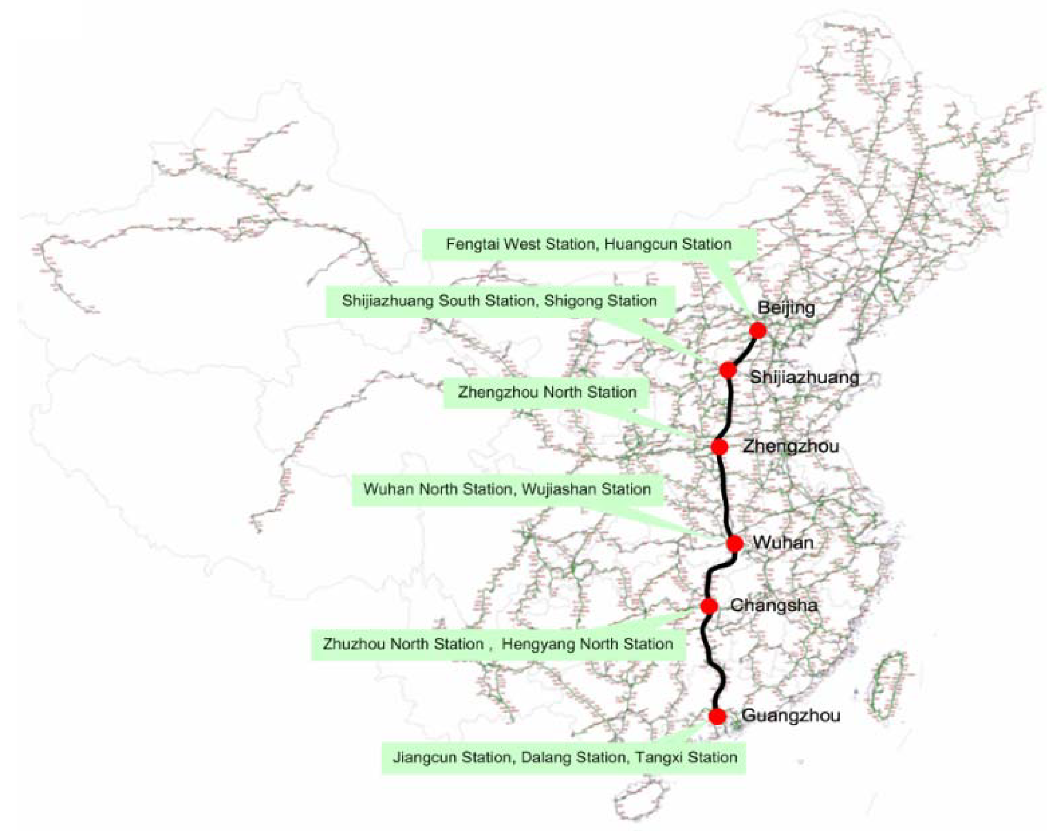
Here, we make a numerical example analysis based on the railway corridor called “Beijing–Guangzhou Railway Line” (see Figure 2), which is one of the most important north–south rail lines in China. The route, from Beijing to Guangzhou, has a total length of 2324 km. It connects six provincial capitals or municipalities and many large- and medium-sized cities, and it is one of the busiest major railways in China. The goods transported to the south on the Beijing–Guangzhou railway mainly include coal, steel, petroleum, timber and export materials. Relatively speaking, the proportion of high value-added goods to the north is higher than to the south. Therefore, this paper uses the northward direction of the Beijing–Guangzhou railway as an example for analysis. This route passes through many important railway hubs, including Guangzhou railway hub (H1), Changsha railway hub (H2), Wuhan railway hub (H3), Zhengzhou railway hub (H4), Shijiazhuang railway hub (H5), and Beijing railway hub (H6).

5.1. Parameters of the Model

The freight demand, volume, prescribed transit time and costs for each railway hub are shown in

Table 3. Information of shipments.

$\mathit{g}$	${\mathit{o}}_{\mathit{g}}$	${\mathit{d}}_{\mathit{g}}$	${\mathit{N}}_{\mathit{g}}$	${\mathit{T}}_{\mathit{g}}$	${\mathit{R}}_{\mathit{g}}$	$\mathit{g}$	${\mathit{o}}_{\mathit{g}}$	${\mathit{d}}_{\mathit{g}}$	${\mathit{N}}_{\mathit{g}}$	${\mathit{T}}_{\mathit{g}}$	${\mathit{R}}_{\mathit{g}}$
F01	H1	H2	4.72	20	5598	F30	H1	H6	5.28	72	19892
F02	H1	H2	14.64	72	19770	F31	H1	H6	4.48	72	19808
F03	H1	H2	4.48	26	9201	F32	H2	H3	3.76	24	5211
F04	H1	H3	29.44	36	9567	F33	H2	H3	4.56	24	5577
F05	H1	H3	13.76	34	13146	F34	H2	H4	4.24	29	9157
F06	H1	H3	7.76	60	16363	F35	H2	H4	3.76	48	12373
F07	H1	H3	9.04	60	16603	F36	H2	H5	13.68	60	12614
F08	H1	H3	2.36	72	28534	F37	H2	H5	7.76	45	14434
F09	H1	H3	7.68	72	19929	F38	H2	H5	5.2	72	16645
F10	H1	H4	17.52	72	19854	F39	H2	H5	5.04	60	16561
F11	H1	H4	2.15	72	28428	F40	H2	H6	25.92	24	19892
F12	H1	H4	11.28	24	5673	F41	H2	H6	19.6	43	19808
F13	H1	H5	8.56	36	9276	F42	H2	H6	10.4	46	5211
F14	H1	H5	5.36	48	9642	F43	H2	H6	7.28	60	5577
F15	H1	H5	5.12	36	13222	F44	H2	H6	4.96	65	9157
F16	H1	H5	3.76	60	16439	F45	H2	H6	3.68	56	12373
F17	H1	H5	3.84	60	16679	F46	H3	H5	26.96	24	12614
F18	H1	H5	7.28	72	19694	F47	H3	H5	4.8	32	14434
F19	H1	H6	4.16	72	19853	F48	H3	H5	5.76	26	16645
F20	H1	H6	8.72	72	28427	F49	H3	H5	18.4	48	16561
F21	H1	H6	3.64	72	28321	F50	H3	H6	12.24	48	8119
F22	H1	H6	17.44	72	19779	F51	H3	H6	7.6	36	11336
F23	H1	H6	37.68	24	5560	F52	H3	H6	6.64	24	11576
F24	H1	H6	25.84	36	9163	F53	H3	H6	5.92	36	13396
F25	H1	H6	19.36	65	9529	F54	H3	H6	5.92	48	13322
F26	H1	H6	18.88	48	13108	F55	H3	H6	4.72	36	13237
F27	H1	H6	14.72	58	16325	F56	H4	H6	4.72	36	7732
F28	H1	H6	8.72	48	16565	F57	H4	H6	4.48	36	7973
F29	H1	H6	5.52	72	19966	F58	H4	H6	3.84	36	9793

. As can be seen in the table, there is a total of 58 flows, with the flow ID from F01 to F58 corresponding to $g$ = 1 to 58. The freight cost $R_g$ is based on the Chinese Railway Tariff (see the data published on the website of 12306) and the transportation distance of shipment $g$. The car volume and freight prescribed transit time are analyzed and speculated based on historical data. Column $o_g$ in Table 3 shows the origin hub of the flow and column $d_g$ indicates the destination hub of the flow. The unit of car volume $N_g$ is car, the unit of freight transportation prescribed time $T_g$ is hour, and the unit of freight cost $R_g$ is CNY/car.

The parameters of all potential train service arcs in the railway network are listed in

Table 4. Information of train services.

$\mathit{m}$	${\mathit{s}}_{\mathit{m}}$	${\mathit{t}}_{\mathit{m}}$	${\mathit{\tau }}_{\mathit{m}}^{\mathit{l}}$			Distance (km)
			$\mathit{l}\mathbf{=}\mathbf{1}$	$\mathit{l}\mathbf{=}\mathbf{2}$	$\mathit{l}\mathbf{=}\mathbf{3}$
A01	H1	H2	10.8	6.9	5	648
A02	H1	H3	18.4	11.6	8.5	1101
A03	H1	H4	26.7	16.9	12.3	1599
A04	H1	H5	33.4	21.1	15.4	2000
A05	H1	H6	38.2	24.2	17.7	2290
A06	H2	H3	7.6	4.8	3.5	453
A07	H2	H4	15.9	10.1	7.4	951
A08	H2	H5	22.6	14.3	10.4	1352
A09	H2	H6	27.4	17.3	12.7	1642
A10	H3	H4	8.3	5.3	3.9	498
A11	H3	H5	15	9.5	7	899
A12	H3	H6	19.9	12.6	9.2	1189
A13	H4	H5	6.7	4.3	3.1	401
A14	H4	H6	11.6	7.3	5.4	691
A15	H5	H6	4.9	3.1	2.3	290

. The columns $s_m$ and $t_m$ in Table 4 represent the origin and destination of the potential train service arc $m$, respectively. The column ${\tau }_m^l$ represents the running time on arc $m$ of the train at the different speed levels, respectively. Specifically, $l=1$ denotes the speed of the train at 80 km/h, $l=2$ denotes the speed of the train at 120 km/h and $l=3$ denotes the speed of the train at 160 km/h. The last column is the mileages for each potential train service arc.

According to the railway operation engineer suggestions, ten train operation plans are generated for the upper model. We present them by assigning values to parameter ${\alpha }_{ijm}^{l\mathbb{P}}{y}_{ij}^{l\mathbb{P}}$ (see Appendix A). In this way, there exists lots of train service arcs in each plan, e.g., the service arc A01 from hub H1 to hub H2 will be provided by train t1, t2, t4, t6 and t12. In order to facilitate solving the model, let (the origin of train service arc, the destination of train service arc, time consumption and train) denote the train service arc, e.g., (H1, H2, 10.8, t1) represents that the service arc from H1 to H2 takes 10.8 h and it is provided by train t1 in train operation plan I.

The cost of express cargo train includes two parts, the first one is the fixed costs, and the second is the variable costs. Specifically, the fixed cost includes the expenditure for the train at the departure station and the running expenditure, and the variable cost is the expenditure of stops along the itinerary. At the departure railway hub, the expenditure for the train in the three speed levels is 4000 CNY, 4500 CNY and 5000 CNY, respectively. The running fee rate for the three speed levels is 1, 1.2 and 2 per kilometer. The expenditure of the train at each stop is 10% of the costs at the departure station.

When a car is transferred from one train to another train, it usually takes approximately ten hours according to the statistics of the main railway hubs in China’s railway system. The reclassification delay ${\tau }_{mn}^k,m(t)\ne n(t),k\in V$ is influenced by capacity of the railway hub $k$. However, the transfer time ${\tau }_{mn}^k,m(t)=n(t),k\in V$ between two arcs belonging to the same train is significantly less than the transfer time ${\tau }_{mn}^k,m(t)\ne n(t),k\in V$ between two arcs belonging to different trains.

Table 5. Transfer time between arc $m$ and arc $n$ in railway hub $k$.

$\mathit{k}$	${\mathit{\tau }}_{\mathit{m}\mathit{n}}^{\mathit{k}}\mathbf{,}\mathit{m}\mathbf{(}\mathit{t}\mathbf{)}\mathbf{\ne }\mathit{n}\mathbf{(}\mathit{t}\mathbf{)}$	${\mathit{\tau }}_{\mathit{m}\mathit{n}}^{\mathit{k}}\mathbf{,}\mathit{m}\mathbf{(}\mathit{t}\mathbf{)}\mathbf{=}\mathit{n}\mathbf{(}\mathit{t}\mathbf{)}$
H1	12.2	2.4
H2	11.1	1.9
H3	7.8	1.3
H4	10	2.3
H5	17.7	3.5
H6	9.9	1.6

shows the values of the time delay ${\tau }_{mn}^k,k\in V$ in hub $k$. The unit of parameter ${\tau }_{mn}^k,k\in V$ is hour.

For example, a shipment from hub H1 to hub H4 takes train service arc (H1, H2, 10.8, t1) from hub H1 to hub H2, takes train service arc (H2, H3, 7.6, t2) from hub H2 to hub H3, and takes train service arc (H3, H4, 8.3, t2) from hub H3 to hub H4 under the train operation plan I. Because of the goods flow needs to be reclassified in hub H2, it will take 11.1 h. However, the goods flow is forced to stop in hub H3 on the train t2, another 1.3 h is needed. Therefore, it will take 10.8 + 11.1 + 7.6 + 1.3 + 8.3 = 39.1 h from hub H1 to H4 for the shipment. In addition, the maximum capacity for one express cargo train is set as 50 cars, i.e., $C_m^{l\mathbb{P}}$ = 50.

The proposed models, including the nonlinear model (NLP) and the linear model (LP), are solved by Gurobi 7.5.2, and all the computational experiments are coded in Python 2.7 and implemented within Spyder 3.1.4 on a laptop with Intel Core i7-6700U CPU and 8 GB RAM. The termination rules for all models are setup with a solver relative gap of 0 in Spyder 3.1.4.

5.2. Computational Performance of the Proposed Model

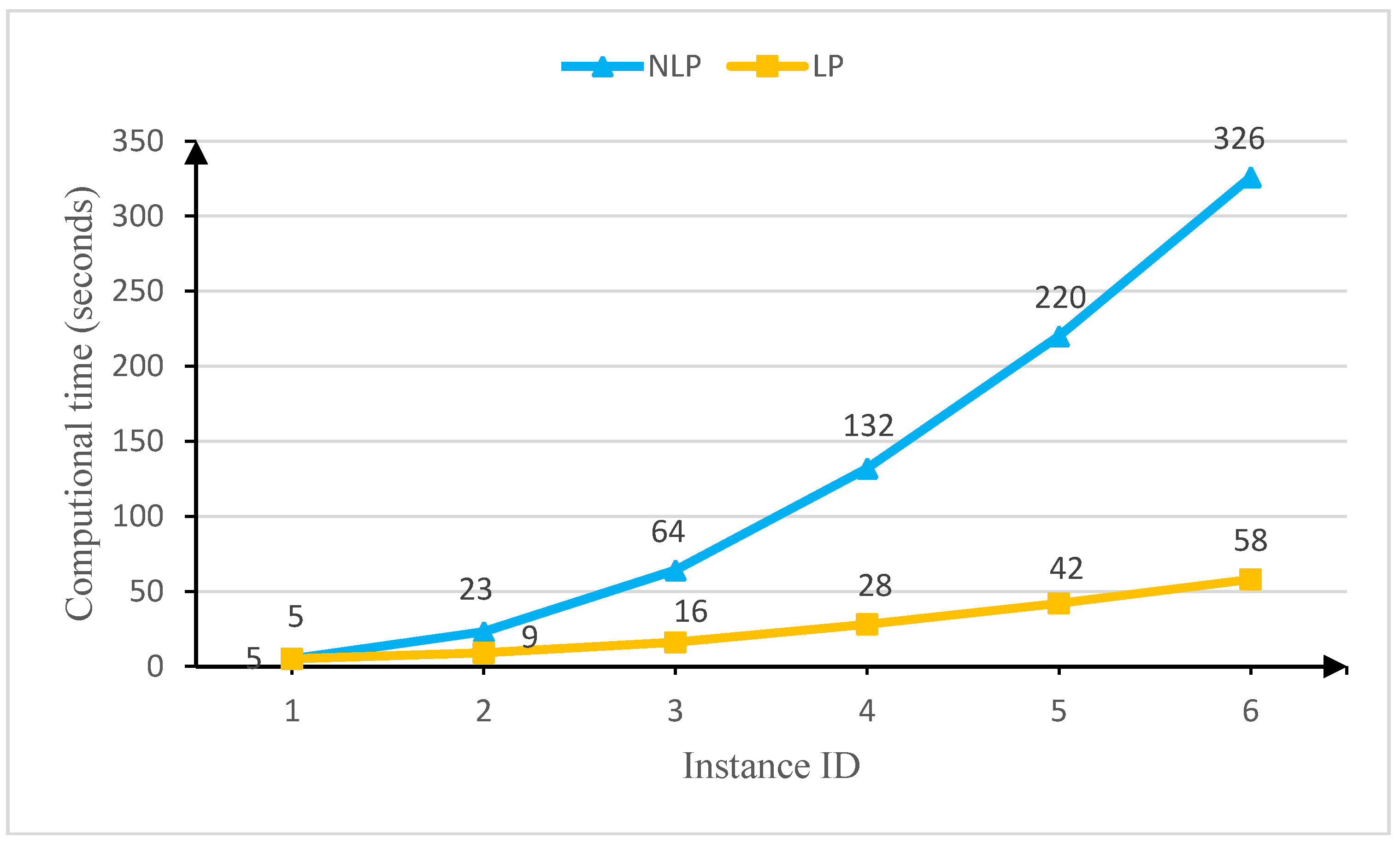
This section aims to test the computational efficiency and effectiveness of the proposed lower-level models, including the nonlinear model (NLP) and the linear model (LP). We test six different instances with different number of flows (from 10 to 58) under train operation plan I. All of the instances data come from Table 3. The parameters for each instance are listed in

Table 6. Problem instances.

Instance ID	The Number of the Flows
1	10 (F01–F10)
2	20 (F01–F20)
3	30 (F01–F30)
4	40 (F01–F40)
5	50 (F01–F50)
6	58 (F01–F58)

. The other parameters can be found in Section 5.1.

Figure 3 shows that the increment in problem size leads to significantly longer computational time, especially for the NLP. The time consumed for the nonlinear model increases exponentially with the expansion of the problem scale, while the proposed linear model increases slowly. It is speculated that linear model has a higher computational efficiency.

5.3. Computational Results and Analysis

All the above instances based on the Beijing–Guangzhou railway line can be solved to optimality after running for about 10 min. The optimal objective function value and transportation demand satisfaction rate of each train operation plan are listed in

Table 7. The optimal objective function value for the different plans.

Plan	$\mathit{Z}$	${\displaystyle \mathbf{\sum }_{\mathit{g}\mathbf{\in }\mathit{G}}{\mathit{N}}_{\mathit{g}}{\mathit{\xi }}_{\mathit{g}}}\mathbf{/}{\displaystyle \mathbf{\sum }_{\mathit{g}\mathbf{\in }\mathit{G}}{\mathit{N}}_{\mathit{g}}}$
I	−12,285,301.68 CNY	100%
II	−10,829,293.23 CNY	87.41%
III	−11,426,699.99 CNY	91.36%
IV	−12,091,374.86 CNY	98.91%
V	−12,282,876.71 CNY	100%
VI	−11,953,287.68 CNY	97.20%
VII	−11,953,287.68 CNY	97.20%
VIII	−12,281,774.42 CNY	100%
IX	−12,284,106.74 CNY	100%
X	−12,284,004.98 CNY	100%

.

By comparing the optimal objective function values for each train operation plan, we find the plan I is the most profitable. A total of 764.03 cars were involved in the calculation of the 58 flows, and the results show that all cars could be delivered to their destinations within the prescribed transit time, accounting for 100% of the total transportation demand. The detailed optimal train operation plan (Plan I) including origin hub, destination hub, speed level and intermediate stops can be found in

Table A1. Train operation plans.

Plan	$\mathit{i}$	$\mathit{j}$	$\mathit{l}$	01	02	03	04	05	06	07	08	09	10	11	12	13	14	15
I	H1	H4	1	1	0	0	0	0	0	1	0	0	0	0	0	0	0	0
	H1	H4	1	1	0	0	0	0	1	0	0	0	1	0	0	0	0	0
	H1	H5	1	0	1	0	0	0	0	0	0	0	0	1	0	0	0	0
	H1	H5	1	1	0	0	0	0	0	0	1	0	0	0	0	0	0	0
	H1	H6	1	0	0	0	0	1	0	0	0	0	0	0	0	0	0	0
	H1	H6	1	1	0	0	0	0	0	0	0	1	0	0	0	0	0	0
	H1	H6	1	0	0	1	0	0	0	0	0	0	0	0	0	0	1	0
	H1	H3	2	0	1	0	0	0	0	0	0	0	0	0	0	0	0	0
	H1	H5	2	0	0	0	1	0	0	0	0	0	0	0	0	0	0	0
	H1	H6	2	0	0	0	0	1	0	0	0	0	0	0	0	0	0	0
	H1	H6	2	0	1	0	0	0	0	0	0	0	0	0	1	0	0	0
	H1	H6	2	1	0	0	0	0	0	0	0	1	0	0	0	0	0	0
	H1	H6	3	0	0	0	0	1	0	0	0	0	0	0	0	0	0	0
II	H1	H3	1	1	0	0	0	0	1	0	0	0	0	0	0	0	0	0
	H1	H4	1	0	0	1	0	0	0	0	0	0	0	0	0	0	0	0
	H1	H5	1	0	1	0	0	0	0	0	0	0	0	1	0	0	0	0
	H1	H5	1	1	0	0	0	0	0	0	1	0	0	0	0	0	0	0
	H1	H6	1	0	0	0	0	1	0	0	0	0	0	0	0	0	0	0
	H1	H6	1	1	0	0	0	0	0	0	0	1	0	0	0	0	0	0
	H1	H3	2	0	1	0	0	0	0	0	0	0	0	0	0	0	0	0
	H1	H5	2	0	0	0	1	0	0	0	0	0	0	0	0	0	0	0
	H1	H6	2	1	0	0	0	0	0	0	0	1	0	0	0	0	0	0
	H1	H6	3	0	0	0	0	1	0	0	0	0	0	0	0	0	0	0
III	H1	H3	1	1	0	0	0	0	1	0	0	0	0	0	0	0	0	0
	H1	H4	1	0	0	1	0	0	0	0	0	0	0	0	0	0	0	0
	H1	H4	1	1	0	0	0	0	0	1	0	0	0	0	0	0	0	0
	H1	H5	1	0	1	0	0	0	0	0	0	0	0	1	0	0	0	0
	H1	H5	1	1	0	0	0	0	0	0	1	0	0	0	0	0	0	0
	H1	H6	1	0	0	0	0	1	0	0	0	0	0	0	0	0	0	0
	H1	H6	1	1	0	0	0	0	0	0	0	1	0	0	0	0	0	0
	H1	H3	2	0	1	0	0	0	0	0	0	0	0	0	0	0	0	0
	H1	H5	2	0	0	0	1	0	0	0	0	0	0	0	0	0	0	0
	H1	H6	2	1	0	0	0	0	0	0	0	1	0	0	0	0	0	0
	H1	H6	3	0	0	0	0	1	0	0	0	0	0	0	0	0	0	0
IV	H1	H4	1	0	0	1	0	0	0	0	0	0	0	0	0	0	0	0
	H1	H4	1	1	0	0	0	0	0	1	0	0	0	0	0	0	0	0
	H1	H5	1	0	1	0	0	0	0	0	0	0	0	1	0	0	0	0
	H1	H5	1	1	0	0	0	0	0	0	1	0	0	0	0	0	0	0
	H1	H6	1	0	1	0	0	0	0	0	0	0	0	0	1	0	0	0
	H1	H6	1	1	0	0	0	0	0	0	0	1	0	0	0	0	0	0
	H1	H3	2	0	1	0	0	0	0	0	0	0	0	0	0	0	0	0
	H1	H5	2	0	0	0	1	0	0	0	0	0	0	0	0	0	0	0
	H1	H6	2	0	1	0	0	0	0	0	0	0	0	0	1	0	0	0
	H1	H6	2	1	0	0	0	0	0	0	0	1	0	0	0	0	0	0
	H1	H6	2	0	1	0	0	0	0	0	0	0	1	0	0	1	0	1
	H1	H6	3	0	0	0	0	1	0	0	0	0	0	0	0	0	0	0
V	H1	H3	1	1	0	0	0	0	1	0	0	0	0	0	0	0	0	0
	H1	H4	1	0	0	1	0	0	0	0	0	0	0	0	0	0	0	0
	H1	H4	1	1	0	0	0	0	0	1	0	0	0	0	0	0	0	0
	H1	H5	1	0	1	0	0	0	0	0	0	0	0	1	0	0	0	0
	H1	H5	1	1	0	0	0	0	0	0	1	0	0	0	0	0	0	0
	H1	H6	1	0	1	0	0	0	0	0	0	0	0	0	1	0	0	0
	H1	H6	1	1	0	0	0	0	0	0	0	1	0	0	0	0	0	0
	H1	H3	2	0	1	0	0	0	0	0	0	0	0	0	0	0	0	0
	H1	H5	2	0	0	0	1	0	0	0	0	0	0	0	0	0	0	0
	H1	H6	2	0	1	0	0	0	0	0	0	0	0	0	1	0	0	0
	H1	H6	2	1	0	0	0	0	0	0	0	1	0	0	0	0	0	0
	H1	H6	2	0	1	0	0	0	0	0	0	0	1	0	0	1	0	1
	H1	H6	3	0	0	0	0	1	0	0	0	0	0	0	0	0	0	0
VI	H1	H4	1	0	0	1	0	0	0	0	0	0	0	0	0	0	0	0
	H1	H4	1	1	0	0	0	0	0	1	0	0	0	0	0	0	0	0
	H1	H5	1	0	1	0	0	0	0	0	0	0	0	1	0	0	0	0
	H1	H5	1	1	0	0	0	0	0	0	1	0	0	0	0	0	0	0
	H1	H6	1	0	0	0	0	1	0	0	0	0	0	0	0	0	0	0
	H1	H6	1	1	0	0	0	0	0	0	0	1	0	0	0	0	0	0
	H1	H3	2	0	1	0	0	0	0	0	0	0	0	0	0	0	0	0
	H1	H5	2	0	0	0	1	0	0	0	0	0	0	0	0	0	0	0
	H1	H6	2	0	0	0	0	1	0	0	0	0	0	0	0	0	0	0
	H1	H6	2	0	1	0	0	0	0	0	0	0	0	0	1	0	0	0
	H1	H6	2	1	0	0	0	0	0	0	0	1	0	0	0	0	0	0
	H1	H6	3	0	0	0	0	1	0	0	0	0	0	0	0	0	0	0
VII	H1	H4	1	0	0	1	0	0	0	0	0	0	0	0	0	0	0	0
	H1	H4	1	1	0	0	0	0	0	1	0	0	0	0	0	0	0	0
	H1	H5	1	0	1	0	0	0	0	0	0	0	0	1	0	0	0	0
	H1	H5	1	1	0	0	0	0	0	0	1	0	0	0	0	0	0	0
	H1	H6	1	0	0	0	0	1	0	0	0	0	0	0	0	0	0	0
	H1	H6	1	1	0	0	0	0	0	0	0	1	0	0	0	0	0	0
	H1	H3	2	0	1	0	0	0	0	0	0	0	0	0	0	0	0	0
	H1	H5	2	0	0	0	1	0	0	0	0	0	0	0	0	0	0	0
	H1	H6	2	0	0	0	0	1	0	0	0	0	0	0	0	0	0	0
	H1	H6	2	0	1	0	0	0	0	0	0	0	0	0	1	0	0	0
	H1	H6	2	1	0	0	0	0	0	0	0	1	0	0	0	0	0	0
	H1	H6	3	0	0	0	0	1	0	0	0	0	0	0	0	0	0	0
VIII	H1	H4	1	0	0	1	0	0	0	0	0	0	0	0	0	0	0	0
	H1	H4	1	1	0	0	0	0	0	1	0	0	0	0	0	0	0	0
	H1	H5	1	0	1	0	0	0	0	0	0	0	0	1	0	0	0	0
	H1	H5	1	1	0	0	0	0	0	0	1	0	0	0	0	0	0	0
	H1	H6	1	0	1	0	0	0	0	0	0	0	1	0	0	0	1	0
	H1	H3	2	0	1	0	0	0	0	0	0	0	0	0	0	0	0	0
	H1	H5	2	0	0	0	1	0	0	0	0	0	0	0	0	0	0	0
	H1	H6	2	0	1	0	0	0	0	0	0	0	0	0	1	0	0	0
	H1	H6	2	1	0	0	0	0	0	0	0	1	0	0	0	0	0	0
	H1	H6	3	0	0	0	0	1	0	0	0	0	0	0	0	0	0	0
	H1	H6	3	1	0	0	0	0	1	0	0	0	0	0	1	0	0	0
	H1	H6	3	0	0	1	0	0	0	0	0	0	0	0	0	1	0	1
IX	H1	H4	1	0	0	1	0	0	0	0	0	0	0	0	0	0	0	0
	H1	H4	1	1	0	0	0	0	0	1	0	0	0	0	0	0	0	0
	H1	H5	1	0	1	0	0	0	0	0	0	0	0	1	0	0	0	0
	H1	H5	1	1	0	0	0	0	0	0	1	0	0	0	0	0	0	0
	H1	H6	1	1	0	0	0	0	0	0	0	1	0	0	0	0	0	0
	H1	H6	1	0	1	0	0	0	0	0	0	0	1	0	0	0	1	0
	H1	H3	2	0	1	0	0	0	0	0	0	0	0	0	0	0	0	0
	H1	H5	2	0	0	0	1	0	0	0	0	0	0	0	0	0	0	0
	H1	H6	2	0	0	0	0	1	0	0	0	0	0	0	0	0	0	0
	H1	H6	2	0	1	0	0	0	0	0	0	0	0	0	1	0	0	0
	H1	H6	2	1	0	0	0	0	0	0	0	1	0	0	0	0	0	0
	H1	H6	2	1	0	0	0	0	1	0	0	0	1	0	0	0	1	0
	H1	H6	3	0	0	0	0	1	0	0	0	0	0	0	0	0	0	0
	H1	H6	3	1	0	0	0	0	1	0	0	0	0	0	1	0	0	0
X	H1	H4	1	0	0	1	0	0	0	0	0	0	0	0	0	0	0	0
	H1	H4	1	1	0	0	0	0	0	1	0	0	0	0	0	0	0	0
	H1	H5	1	0	1	0	0	0	0	0	0	0	0	1	0	0	0	0
	H1	H5	1	1	0	0	0	0	0	0	1	0	0	0	0	0	0	0
	H1	H6	1	1	0	0	0	0	0	0	0	1	0	0	0	0	0	0
	H1	H6	1	0	1	0	0	0	0	0	0	0	1	0	0	0	1	0
	H1	H5	2	0	0	0	1	0	0	0	0	0	0	0	0	0	0	0
	H1	H6	2	0	0	0	0	1	0	0	0	0	0	0	0	0	0	0
	H1	H6	2	0	1	0	0	0	0	0	0	0	0	0	1	0	0	0
	H1	H6	2	1	0	0	0	0	0	0	0	1	0	0	0	0	0	0
	H1	H6	2	1	0	0	0	0	1	0	0	0	1	0	0	0	1	0
	H1	H6	3	0	0	0	0	1	0	0	0	0	0	0	0	0	0	0
	H1	H6	3	1	0	0	0	0	1	0	0	0	0	0	1	0	0	0

.

The detailed service arcs selection for each shipment is shown in

Table 8. Results of the car-to-train assignment.

$\mathit{g}$	${\mathit{o}}_{\mathit{g}}$	${\mathit{d}}_{\mathit{g}}$	${\mathit{\xi }}_{\mathit{g}}$	Service Arc	$\mathit{g}$	${\mathit{o}}_{\mathit{g}}$	${\mathit{d}}_{\mathit{g}}$	${\mathit{\xi }}_{\mathit{g}}$	Service Arc
F01	H1	H2	100%	(H1, H2, 10.8, t4)	F30	H1	H6	100%	(H1, H6, 17.7, t13)
F02	H1	H2	100%	(H1, H2, 6.9, t12)	F31	H1	H6	100%	(H1, H6, 17.7, t13)
F03	H1	H2	100%	(H1, H2, 6.9, t12)	F32	H2	H3	100%	(H2, H3, 7.6, t2)
F04	H1	H3	100%	(H1, H3, 18.4, t3)	F33	H2	H3	100%	(H2, H3, 7.6, t2)
F05	H1	H3	100%	(H1, H3, 18.4, t3)	F34	H2	H4	100%	(H2, H4, 15.9, t1)
F06	H1	H3	100%	(H1, H3, 18.4, t3)	F35	H2	H4	100%	(H2, H4, 15.9, t1)
F07	H1	H3	100%	(H1, H3, 11.6, t11)	F36	H2	H5	100%	(H2, H5, 22.6, t4)
F08	H1	H3	100%	(H1, H3, 11.6, t11)	F37	H2	H5	100%	(H2, H5, 22.6, t4)
F09	H1	H3	100%	(H1, H3, 11.6, t8)	F38	H2	H5	100%	(H2, H5, 22.6, t4)
F10	H1	H4	100%	(H1, H4, 26.7, t7)	F39	H2	H5	100%	(H2, H5, 22.6, t4)
F11	H1	H4	100%	(H1, H2, 10.8, t1) (H2, H4, 15.9, t1)	F40	H2	H6	100%	(H2, H6, 27.4, t6)
F12	H1	H4	100%	(H1, H2, 10.8, t2) (H2, H3, 7.6, t2) (H3, H4, 8.3, t2)	F41	H2	H6	100%	(H2, H6, 27.4, t6)
F13	H1	H5	100%	(H1, H3, 18.4, t3) (H3, H5, 15.0, t3)	F42	H2	H6	100%	(H2, H6, 27.4, t6)
F14	H1	H5	100%	(H1, H2, 10.8, t4) (H2, H5, 22.6, t4)	F43	H2	H6	100%	(H2, H6, 17.3, t12)
F15	H1	H5	100%	(H1, H5, 21.1, t9)	F44	H2	H6	100%	(H2, H6, 17.3, t12)
F16	H1	H5	100%	(H1, H5, 21.1, t9)	F45	H2	H6	100%	(H2, H6, 17.3, t12)
F17	H1	H5	100%	(H1, H5, 21.1, t9)	F46	H3	H5	100%	(H3, H5, 15.0, t3)
F18	H1	H5	100%	(H1, H5, 21.1, t9)	F47	H3	H5	100%	(H3, H5, 15.0, t3)
F19	H1	H6	100%	(H1, H6, 38.2, t5)	F48	H3	H5	100%	(H3, H5, 15.0, t3)
F20	H1	H6	100%	(H1, H2, 10.8, t6) (H2, H6, 27.4, t6)	F49	H3	H5	100%	(H3, H5, 15.0, t3)
F21	H1	H6	100%	(H1, H4, 26.7, t7) (H4, H6, 11.6, t7)	F50	H3	H6	100%	(H3, H6, 12.6, t11)
F22	H1	H6	100%	(H1, H6, 24.2, t10)	F51	H3	H6	100%	(H3, H4, 8.3, t2) (H4, H6, 11.6, t6)
F23	H1	H6	100%	(H1, H2, 6.9, t12) (H2, H6, 17.3, t12)	F52	H3	H6	100%	(H3, H6, 12.6, t11)
F24	H1	H6	100%	(H1, H3, 11.6, t11) (H3, H6, 12.6, t11)	F53	H3	H6	100%	(H3, H6, 12.6, t11)
F25	H1	H6	100%	(H1, H6, 24.2, t10)	F54	H3	H6	100%	(H3, H6, 12.6, t11)
F26	H1	H6	100%	(H1, H6, 17.7, t13)	F55	H3	H6	100%	(H3, H6, 12.6, t11)
F27	H1	H6	100%	(H1, H6, 17.7, t13)	F56	H4	H6	100%	(H4, H6, 11.6, t7)
F28	H1	H6	100%	(H1, H6, 17.7, t13)	F57	H4	H6	100%	(H4, H6, 11.6, t7)
F29	H1	H6	100%	(H1, H6, 17.7, t13)	F58	H4	H6	100%	(H4, H6, 11.6, t7)

. There is only one flow, F51, be reclassified that transfer from train t2 to train t6 in hub H4. The total reclassification delay is 76 car-hours (7.6 × 10). The total transfer time without reclassification is 176.963 car-hours, and most of them, approximately 98%, occur in hub H2.

The operating frequency ($f_{ij}^{l\mathbb{P}}$) of each train in Plan I is shown in

Table 9. The operating frequency of each train.

Train	t1	t2	t3	t4	t5	t6	t7	t8	t9	t10	t11	t12	t13
$f_{ij}^{l\mathbb{P}}$	0.88	0.27	1.56	1.23	0.55	1.22	0.73	0.11	0.91	1.20	1.33	0.85	1.19

.

In this experiment, we set the value of $C_m^{l\mathbb{P}}$ to be 50. The actual number of cars in each train can be calculated by $C_m^{l\mathbb{P}}{f}_{ij}^{l\mathbb{P}}$. Take train t1 as an example, the actual number of cars is 44 cars (50 × 0.88) in t1. Meanwhile, the operating frequency becomes 1 in this scenario accordingly.

6. Conclusions

In this paper, a bi-level programming model for express cargo service network design is proposed. The upper-level model forms the optimal decisions in terms of the service characteristics, and the lower-level model carries out the flow distribution according to the train operation plan and service commitments. According to the characteristics of high value-added goods, the prescribed transit time constraint is added to the model, considering both the transportation time on the arcs and the transfer time between arcs. In addition, the arc capacity constraint and flow balance constraint are considered. Moreover, linearization techniques are used to convert the lower-level model to a linear one so that it can be directly solved by a standard optimization solver. Finally, a real-world case study is carried out based on the Beijing–Guangzhou Railway Line, which is one of the busiest railway lines in China. The example consists of six railway hubs and five segments, and we consider the northward direction. The results indicate that the bi-level model has significance in real-life application to the rail express cargos service network design problem. Although the train operation plans come from the upper-level model were developed manually, the results of flow distribution from the lower-level model can serve as a solid aid in improving the quality of train operation planning. In the future, researchers can focus on the joint optimization of the train operation plan and the flow distribution scheme with the three-dimensional bin-packing method. It is also an interesting future work of applying multiobjective optimization methods (e.g., Pareto-optimization approaches) to solve the railway express cargo service network design problem.

References

- Liu, C.; Lin, B.L.; Wang, J.X.; Liu, S.; Wu, J.; Li, J. Flow assignment model for quantitative analysis of diverting bulk freight from road to railway. PLoS ONE 2017, 12, e0182179. [Google Scholar] [CrossRef] [PubMed]
- Ahuja, R.; Magnanti, T.; Orlin, J. Network flows: Theory, algorithms, and applications. J. Oper. Res. Soc. 1993, 45, 791–796. [Google Scholar] [CrossRef]
- Crainic, T.G.; Kim, K.H. Chapter 8 intermodal transportation. In Transportation: Handbooks in Operations Research and Management Science; Barnhart, C., Laporte, G., Eds.; Elsevier: Amsterdam, The Netherlands, 2006; Volume 14, pp. 189–284. ISBN 9780080467436. [Google Scholar]
- Crainic, T. Long-Haul Freight Transportation. In Handbook of Transportation Science, International Series in Operations Research & Management Science; Hall, R.W., Ed.; Springer: Boston, MA, USA, 2003; Volume 56, pp. 451–516. ISBN 9781402072468. [Google Scholar]
- Crainic, T.; Ferland, J.A.; Rousseau, J.M. A tactical planning model for rail freight transportation. Transp. Sci. 1984, 18, 165–184. [Google Scholar] [CrossRef]
- Campetella, M.; Lulli, G.; Pietropaoli, U.; Ricciardi, N. Freight Service Design for the Italian Railways Company. In Proceedings of the ATMOS 6th Workshop on Algorithmic Methods and Models for Optimization Railways, Zurich, Switzerland, 14 September 2006. [Google Scholar]
- Ahuja, R.K.; Jha, K.C.; Liu, J. Solving real-life railroad blocking problems. Interfaces 2007, 47, 404–419. [Google Scholar] [CrossRef]
- Ceselli, A.; Gatto, M.; Lübbecke, M.E.; Nunkesser, M. Optimizing the Cargo Express Service of Swiss Federal Railways. Transp. Sci. 2008, 42, 450–465. [Google Scholar] [CrossRef] [Green Version]
- Lin, B.L.; Wang, Z.M.; Ji, L.J.; Tian, Y.M.; Zhou, G.Q. Optimizing the freight train connection service network of a large-scale rail system. Transp. Res. B Meth. 2012, 46, 649–667. [Google Scholar] [CrossRef]
- Zhu, E.; Cranic, T.G.; Gendreau, M. Scheduled Service Network Design for Freight Rail Transportation. Oper. Res. 2014, 62, 383–400. [Google Scholar] [CrossRef]
- Newton, H.N.; Barnhart, C.; Vance, P.H. Constructing railroad blocking plans to minimize handling costs. Transport. Sci. 1998, 32, 330–345. [Google Scholar] [CrossRef]
- Barnhart, C.; Jin, H.; Vance, P. Railroad blocking: A network design application. Oper. Res. 2000, 48, 603–614. [Google Scholar] [CrossRef]
- Barnhart, C.; Krishnan, N.; Kim, D.; Ware, K. Network design for express shipment delivery. Comput. Optim. Appl. 2002, 21, 239–262. [Google Scholar] [CrossRef]
- Kim, D.; Barnhart, C.; Ware, K.; Reinhardt, G. Multimodal express package delivery: A service network design application. Transp. Sci. 1999, 33, 391–407. [Google Scholar] [CrossRef]
- Armacost, A.P.; Barnhart, C.; Ware, K.A. Composite variable formulations for express shipment service network design. Transp. Sci. 2002, 36, 1–20. [Google Scholar] [CrossRef]
- Yang, T.H.; Chen, C.C. Air Freight Service Network Design for Stochastic Demand. In Proceedings of the IEEE/INFORMS, International Conference on Service Operations, Logistics and Informatics, Chicago, IL, USA, 22–24 July 2009; IEEE: Washington, DC, USA, 2009. [Google Scholar]
- Christiansen, M.; Fagerholt, K.; Nygreen, B.; Ronen, D. Chapter 4 maritime transportation. In Handbooks in Operations Research and Management Science; Barnhart, C., Laporte, G., Eds.; Elsevier: Amsterdam, The Netherlands, 2006; Volume 14, pp. 189–284. ISBN 9780080467436. [Google Scholar]
- Wang, D.Z.W.; Lo, H.K. Multi-fleet ferry service network design with passenger preferences for differential services. Transp. Res. B Meth. 2008, 42, 798–822. [Google Scholar] [CrossRef]
- Nourbakhsh, S.M.; Ouyang, Y. A structured flexible transit system for low demand areas. Transp. Res. B Meth. 2012, 46, 204–216. [Google Scholar] [CrossRef]
- Bai, R.; Wallace, S.W.; Li, J.; Chong, A.Y.L. Stochastic service network design with rerouting. Transp. Res. B Meth. 2014, 60, 50–65. [Google Scholar] [CrossRef] [Green Version]
- Ji, S.F.; Luo, R.J. A hybrid estimation of distribution algorithm for multi-objective multi-sourcing intermodal transportation network design problem considering carbon emissions. Sustainability 2017, 9, 1133. [Google Scholar] [CrossRef]
- Di, X.; Ma, R.; Liu, H.X.; Ban, X.G. A link-node reformulation of ridesharing user equilibrium with network design. Transp. Res. B Meth. 2018, 112, 230–255. [Google Scholar] [CrossRef]
- Liu, J.T.; Zhou, X.S. Capacitated transit service network design with boundedly rational agents. Transp. Res. B Meth. 2016, 93, 225–250. [Google Scholar] [CrossRef] [Green Version]
- Lin, B.L. A study of car-to-train assignment problem for rail express cargos on scheduled and unscheduled train service network. arXiv 2018, arXiv:1803.05760v1. [Google Scholar]
Figure 1.
The railway train service network.
Figure 2.
Beijing–Guangzhou railway line.
Figure 3.
Comparison of computational time between the nonlinear and linear models.