Incremental Spectral Clustering via Fastfood Features and Its Application to Stream Image Segmentation

Abstract

We propose an incremental spectral clustering method for stream data clustering and apply it to stream image segmentation. The main idea in our work consists of generating the data points in the kernel space by Fastfood features and iteratively calculating the eigendecomposition of data. Compared with the popular Nyström-based approximation, our work accesses each data point only once while Nyström, in particular the sampling scheme, will go through the entire dataset first and calculate the embeddings of data points with a second visit. As a result, our method is able to learn data partitions incrementally and improve eigenvector approximation with more and more data seen from a stream. By contrast, the performance of the standard Nyström is fixed when the sample set is selected. Experimental results show the superiority of our method.

1. Introduction

In the last decade, clustering methods are widely used in image processing and data mining, such as image segmentation [1], image matting [2], path planing [3] and thermal error modeling [4]. Due to its advantages in clustering accuracy, spectral clustering plays an important role in data partition [5]. It has demonstrated success in revealing the underlying complicated, in most cases non-linear, structure of real-world dataset. However, spectral clustering is known for its shortage of huge computational burden, in particular of $O\left(n^3\right)$ in computational complexity of a dataset with volume n. The cubic growth on time cost prevents spectral clustering from online processing with stream data.

A popular way to accelerate spectral clustering is the Nyström approximation that approximates the eigenvectors of the kernel matrix by a subset, typically known as the training set, of data points. In general, Nyström method requires $O(m^3+n{m}^2)$ in time cost [6], where m is the volume of the training data. As to memory storage, Nyström needs to hold the sampled landmark points in main memory, typically with $O\left(nm\right)$. When n is large, the main memory may not be sufficient. Another disadvantage of Nyström for stream data is the sampling process which is essential for the approximation accuracy in Nyström. Popular sampling methods, such as the k-means or the kernel k-means sampling, need to go through the entire input data first and search for the optimal landmark points. In stream-data and memory-limited tasks where only current data are temporally stored, one method is expected to make the optimal clustering according to iteratively improve its learnt model with the coming data stream. However, the sampling process in Nyström often finds difficulty to do so. Incremental clustering method [7,8], as a promising solution, is able to incrementally partition data points and obtain the up-to-now clustering results according the seen data.

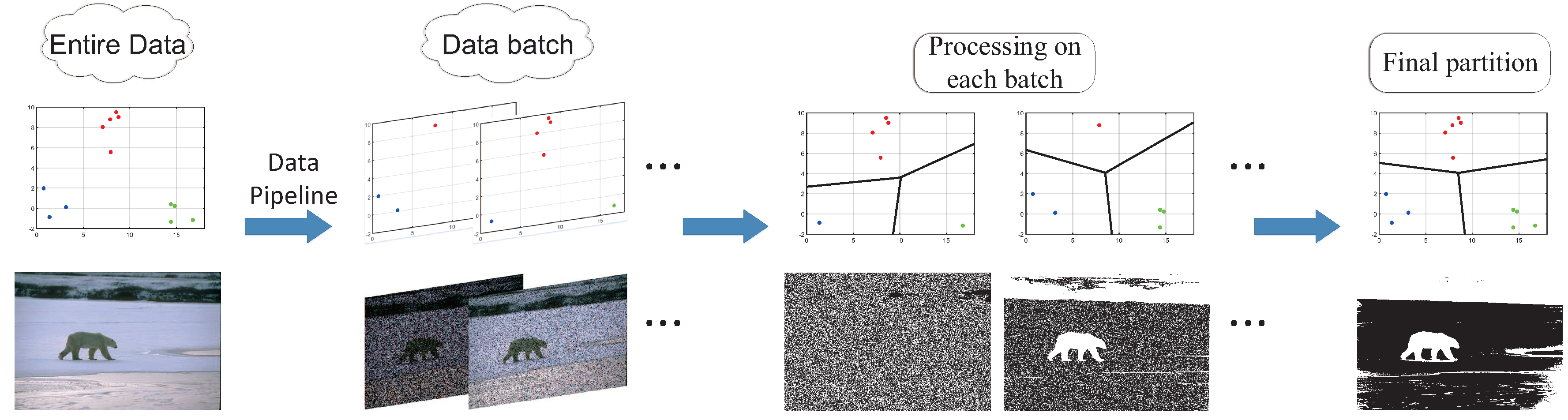
In this paper, we propose a new framework for approximating the eigenvectors of the kernel matrix. Compared with the Nyström methods, our method shows its superiority in memory usage: our method requires a constant occupation of memory, $O\left(D^2\right)$, where D is the dimension of Fastfood features [9] and is fixed by users. One promoting property of our method is the absence of memory storage with respect to data size n, indicating the stream-data-friendly fashion of our method. Actually, we only hold a $D\times D$ matrix in memory and update this fixed-size matrix in data stream. We show a demonstration of the stream data processing in Figure 1. In Figure 1, the entire dataset (on the left) is separated into many subsets, or batches. A processing unit loads and runs clustering on one batch after another (in the middle) and, once all data points are seen, returns the final partition according to all batch results (on the right). As its theoretical foundation, we need to solve the eigenvectors, which are used in spectral clustering for the final partition, in an incremental fashion. Since most processing units in stream data clustering are memory-sensitive, it is strongly recommended to avoid any storage of history data.

Our main idea consists of the employment of Fastfood features, by which we are able to explicitly represent data points in the kernel space. Denote the $D\times n$ matrix X as the data points in the kernel space with one column standing for one data point. Spectral clustering, in this manner, requires solving the eigensystem of the $n\times n$ kernel matrix $K=X^{T}X$, with n iteratively increasing in case of stream data tasks. Instead of studying K, we focus on the $D\times D$ matrix $G=X{X}^T$, which has a constant size even if n increases. We solve the eigensystem of K from that of G and apply our method in data stream clustering.

Our contributions include the followings:

• We propose an incremental spectral clustering method with a constant memory requirement. Thus, our method is suitable for stream data clustering.
• We solve the eigensystem of kernel matrix K from another matrix, titled G in our works, a process in return benefiting us in both time cost and memory storage.

The rest of this paper is organized as follows. Section 2 reviews the related works in large-scale and stream data spectral clustering. Our algorithm is described in Section 3. Section 4 presents the experimental results on several datasets. We conclude this paper in Section 5.

2. Related Works

Spectral clustering problem is always identical to solve eigenvectors of a kernel matrix $K\in {\mathbb{R}}^{n\times n}$, which is conducted to estimate the similarity among data points. The eigendecomposition of K always requires $O\left(n^3\right)$ in time cost and $O\left(n^2\right)$ in memory. To accelerate the eigendecomposition on K, the Nyström method is popular [10,11]. The basic idea of Nsytröm is to sample some training data points and build the low-rank approximation to K from the training set.

2.1. Nyström

Nyström is the most popular method to generate the low-rank approximation to a kernel matrix. Suppose K are organized according to the training set and the testing set, respectively, and

$$K=\left[\begin{array}{cc}W& C^T\\ C& K_2\end{array}\right],E=\left[\begin{array}{c}W\\ C\end{array}\right]$$

(1)

where W is the similarity matrix among the training data, C the similarity matrix of the remaining data to the sample set, and $K_2$ is the similarity among the remaining data.

Nyström uses the $m\times m$ matrix W and $n\times m$ matrix C to approximate K by

$$K\approx \tilde{K}=C{W}^{+}{C}^T$$

(2)

and approximates the top k eigenvalues ${\mathsf{\Lambda }}_k$ and eigenvectors $V_k$ by

$${\tilde{\mathsf{\Lambda }}}_k=\frac{n}{m}{\mathsf{\Lambda }}_{Wk}$$

(3)

$${\tilde{V}}_k=\sqrt{\frac{m}{n}}C{V}_{Wk}{\left({\mathsf{\Lambda }}_{Wk}\right)}^{-1}$$

(4)

where $W^{+}$ represents the Moore–Penrose pseudo-inverse of W, and ${\mathsf{\Lambda }}_{Wk}$ are the top k eigenvalues of the sampled kernel matrix W with corresponding eigenvectors $V_{Wk}$.

2.2. CUR Approximation

Besides the Nyström method, CUR decomposition is also a popular fashion for kernel approximation. CUR attempts to form three new matrices, C, R and U, where C haa c columns picking from K, R has r rows of K and U is the intersection matrix. Then, CUR will minimize the approximation error $\parallel K-CUR\parallel$.

Various CUR methods have been proposed in recent years. Wang et al. proposed an adaptive sampling method for CUR decomposition [12]. They first employed the near-optimal column selection algorithm [13] to select c columns to form both C and the first c rows in R. Then, they selected the remaining $r-c$ rows according to the residual. They iteratively performed such column–row picking step for a given number of times and showed that the expected error is proportional to $\parallel K-K_c\parallel$, where $K_c$ is the best rank-c approximation of K from SVD decomposition.

Beyond Nyström and CUR, there are several approximation methods, such as Orthogonal Matching Pursuit (OMP) [14,15]. OMP attempts to select a sparse dictionary for data representation and is widely used in communication and signal processing. OMP searches for the optimal projections of data onto an over-completed dictionary in a greedy fashion.

2.3. Random Kitchen Sinks and Fastfood Features

Denote ${\left\{x_i\right\}}_{i=1}^n$ as the input data points. The corresponding kernel matrix is thus $K\in {\mathbb{R}}^{n\times n}$. Random Kitchen Sinks (RKS) attempts to solve $X\in {\mathbb{R}}^{D\times n}$ such that $K=X^{T}X$ where D is the dimension of the kernel space. One column in X indicates one data point in the kernel space. As one efficient solution, RKS [16] approximates X with $\mathsf{\Phi }\left(x\right)$,

$$\begin{array}{c}{X}^T\approx \mathsf{\Phi }{(x)}^T=\hfill \\ \sqrt{\frac{2}{D}}\left[\begin{array}{c}\cos ({\omega }_1^T{x}_1)\sin ({\omega }_1^T{x}_1)\cdots \cos ({\omega }_{\frac{D}{2}}^T{x}_1)\sin ({\omega }_{\frac{D}{2}}^T{x}_1)\\ \cos ({\omega }_1^T{x}_2)\sin ({\omega }_1^T{x}_2)\cdots \cos ({\omega }_{\frac{D}{2}}^T{x}_2)\sin ({\omega }_{\frac{D}{2}}^T{x}_2)\\ ⋮\\ \cos ({\omega }_1^T{x}_n)\sin ({\omega }_1^T{x}_n)\cdots \cos ({\omega }_{\frac{D}{2}}^T{x}_n)\sin ({\omega }_{\frac{D}{2}}^T{x}_n)\end{array}\right]\hfill \end{array}$$

(5)

where $\omega$ is the Fourier frequency chosen randomly from $\mathcal{N}(0,{\sigma }^{-2})$ and $\sigma$ is the Gaussian kernel scale parameter, $\ker (x,y)=\exp (-\parallel x-y{\parallel }^2/2{\sigma }^2)$. As shown in [17], the approximation error is related to D, where a large D will improve the approximation accuracy.

Other than RKS, Fastfood features [9] are shown with more efficient in both time cost and memory usage. Fastfood features replace the $\{\cos ,\sin \}$ part in RKS with

$$V=\frac{1}{\sigma \sqrt{d}}SHG\mathsf{\Pi }HB$$

(6)

where $H=H_d$ is the $d\times d$ Walsh–Hadamard matrix, $\mathsf{\Pi }\in {\{0,1\}}^{d\times d}$ is a random permutation matrix and S, G and B are all diagonal random matrices where B are uniformly drawn from $\{-1,+1\}$, G has values drawn from a Gaussian distribution and S is a random scaling matrix. Then, the feature mapping of data points are

$$\mathsf{\Phi }\left(x\right)={\left(D\right)}^{-1/2}\exp \left(i\right[Vx\left]\right)$$

(7)

The computational burden of Fastfood features are $O\left(n\log d\right)$ in time and $O\left(n\right)$ in storage [9].

3. Incremental Spectral Clustering via Fastfood

3.1. Main Idea

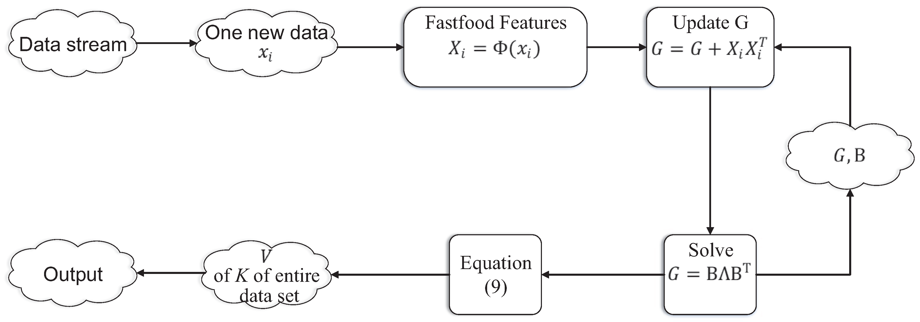
In this section, we propose our main contribution that incrementally calculates the eigensystem of the kernel matrix K. We show our framework in Figure 2.

Denote $K=X^{T}X$ and $G=X{X}^T$. The eigenvector/eigenvalue pairs of the couple matrices can be defined as

$$K:\{v,\lambda \},G:\{\beta ,\gamma \}$$

(8)

Given the eigensystem of both K and G, we can represent v of K by $\beta$ of G, as shown in Theorem 1.

Theorem 1.

Denote the eigensystem the same as shown in Equation (8). Then, $\{v,\lambda \}$ can be represented by $\{\beta ,\gamma \}$ and vice versa,

$$\begin{array}{cc}\hfill v& ={\gamma }^{-1/2}{X}^T\beta \hfill \\ \hfill \beta & ={\lambda }^{-1/2}Xv\hfill \\ \hfill \lambda & =\gamma \hfill \end{array}$$

(9)

Proof. 

To verify whether $\tilde{v}={\gamma }^{-1/2}{X}^T\beta$ is a valid eigenvector of K, we just verify whether $K\tilde{v}=\lambda \tilde{v}$ holds true or not.

$$\begin{array}{cc}\hfill K\tilde{v}& =K{\gamma }^{-1/2}{X}^T\beta \hfill \\ & ={\gamma }^{-1/2}{X}^{T}X{X}^T\beta \hfill \\ & ={\gamma }^{-1/2}{X}^{T}G\beta \hfill \\ & =\gamma X^T{\gamma }^{-1/2}\beta \hfill \\ & =\gamma \tilde{v}\hfill \end{array}$$

(10)

In the second equality of Equation (10), we use the fact that $K=X^{T}X$. To obtain the fourth equality, we employed that $\beta$ is an eigenvector of G with the corresponding eigenvalue $\gamma$. By Equation (10), we show that $\tilde{v}={\gamma }^{-1/2}{X}^T\beta$ is an eigenvector of K with the corresponding eigenvalue $\gamma$. It is easy to verify in the same way that $\beta ={\lambda }^{-1/2}Xv$ is an eigenvector of G with the corresponding eigenvalue $\lambda$. Then, we obtain Equation (9). ☐

By Equation (9), we could solve the eigensystem of K from that of G. Notice that G can be decomposed as the sum of n rank-one matrices as

$$G=\sum _{i=1}^n{X}_i{X}_i^T$$

(11)

where in Equation (11) $X_i$ indicates the i-th column in X.

Equation (11) implies an incremental way in approximating G. Suppose we already have the eigensystem of $G^{\left(n\right)}$ from the leading n data points of a stream, when a new data point $x_{n+1}$ arrives along with its kernel mapping $X_{n+1}=\mathsf{\Phi }\left(x_{n+1}\right)$ from Equation (7), the updated $G^{(n+1)}$ is then

$$G^{(n+1)}=G^{\left(n\right)}+X_{n+1}{X}_{n+1}^T$$

(12)

Notice that, in Equation (12), the size of G is fixed as $D\times D$ through all iterations. Thus, maintaining G in the main memory requires a constant volume.

Denote $\{{\beta }^{\left(n\right)},{\gamma }^{\left(n\right)}\}$ as the eigensystem of $G^{\left(n\right)}$. With the assumption that ${\beta }^{(n+1)}\approx {\beta }^{\left(n\right)}$, we can efficiently solve the updated eigenvectors ${\beta }^{(n+1)}$ by many eigenvector approximation methods, such as power iteration [18]. We summarize our proposed method in Algorithm 1.

3.2. Complexity Analysis

The proposed incremental spectral clustering method in Algorithm 1 shows its advantages over the Nyström methods in both time cost and memory usage. In this section, we give details on both time complexity and memory complexity of our method.

Given n data points in the d-dimensional input space, the Fastfood feature requires $O\left(nd\right)$ operations in generating the $D\times n$ kernel data matrix X. Solving the eigensystem of G is a bottleneck in running time since typically $O\left(D^3\right)$ operations are required to solve the full matrix G. However, in stream data clustering with the assumption that $\beta$ remains stable in coming data, we initialize our $\beta$ with that of the previous results and update $\beta$ in an power-iteration fashion. The actual running time in solving $\beta$ thus is limited. Finally, solving v of K from the learnt $\beta$ takes $O\left(nD\right)$ in time consumption. In summary, the overall running time complexity of the proposed method is $O(nd+D^3)$ and is even much faster if we solve the eigensystem with an efficient eigen-solver. In contrast, the Nyström methods need $O(nmd+m^3+n{m}^2)$ in time complexity where m is the training set volume and is not suitable for incremental clustering.

Algorithm 1 Incremental Spectral Clustering via Fastfood

INPUT: Desired dimension D of Fastfood features, n data points x from a data stream, Gaussian scale parameter $\sigma$, $\beta$ convergence threshold ${ϵ}_{\beta }$. OUTPUT: The approximated eigenvectors v of the $n\times n$ kernel matrix K.  Initialize Fastfood parameters S, H, G and $\mathsf{\Pi }$. Initialize eigenvectors $\beta$ with random values.  Initialize $G^{\left(0\right)}$ with all zero values.  for $i=1$ to n do   Pick the i-th data point $x_i$.   Calculate the $D\times 1$ Fastfood feature vector $X_i$ of $x_i$ with the initialized S, H, G and $\mathsf{\Pi }$.   Update G: $G^{\left(i\right)}=G^{(i-1)}+X_i{X}_i^T$.   repeat    Loop $\beta$: $\beta =G\beta /\parallel G\beta \parallel$.   until $\beta$ converges in ${ϵ}_{\beta }$.  end for  $v=X^T\beta /\parallel X^T\beta \parallel$.

As to memory complexity, our method only upholds the $D\times D$ matrix G and $D\times k$ eigenvectors $\beta$ in memory. Our memory usage thus is constant with respect to data size n. As n increases, our G and $\beta$ are both with fixed size and thus benefit a lot for efficient clustering.

3.3. Comparison with Related Methods

In standard spectral clustering, when a new data point arrives, the corresponding kernel matrix K then becomes $(n+1)\times (n+1)$. The square growth of K in memory storage prevents the standard spectral clustering from any large-scale or stream data tasks. In the proposed method, we replace K with the corresponding G and update G instead in a stream. In our fashion, either G or its eigenvectors $\beta$ are both with fixed size when n increases. Thus, our method is more suitable for stream data clustering than the standard spectral clustering.

Although the Nyström methods are able to accelerate clustering significantly, Nyström may find difficulties in building a proper training set in stream data tasks. The construction of the training set in Nyström prefers to sample as many as possible points from the entire dataset in the purpose of accurately revealing the underlying distribution of data points. In stream data tasks, however, the processing unit is always memory-sensitive and only holds the current points due to memory limitation. The Nyström methods, thus, may suffer from undersampling due to inadequate observations from a data stream.

Compared with standard methods, the proposed incremental spectral clustering method is suitable for stream data clustering, in particular memory-sensitive tasks. The absence of sampling step, as used in Nyström, ensures the ability of our method to process data in one-shot, i.e., without a second visit to each point. In addition, the employment of Fastfood features provides a customized solution to kernel eigenvector decomposition, as shown in Algorithm 1. In this way, users are able to dynamically change the hardware deployment to meet their own memory or accuracy considerations.

4. Experimental Results

We verified the performance of our proposed method on several real-world datasets. We used the Fastfoot Matlab code (https://www.dropbox.com/s/p5vtzqvcdwlswg8/FastMMD.zip) in our work. All experiments were carried out in MATLAB. Our platform running these experiments is a laptop equipped with an Intel 2.66 GHz CPU and a 4 GB RAM.

4.1. Datasets and Competing Methods

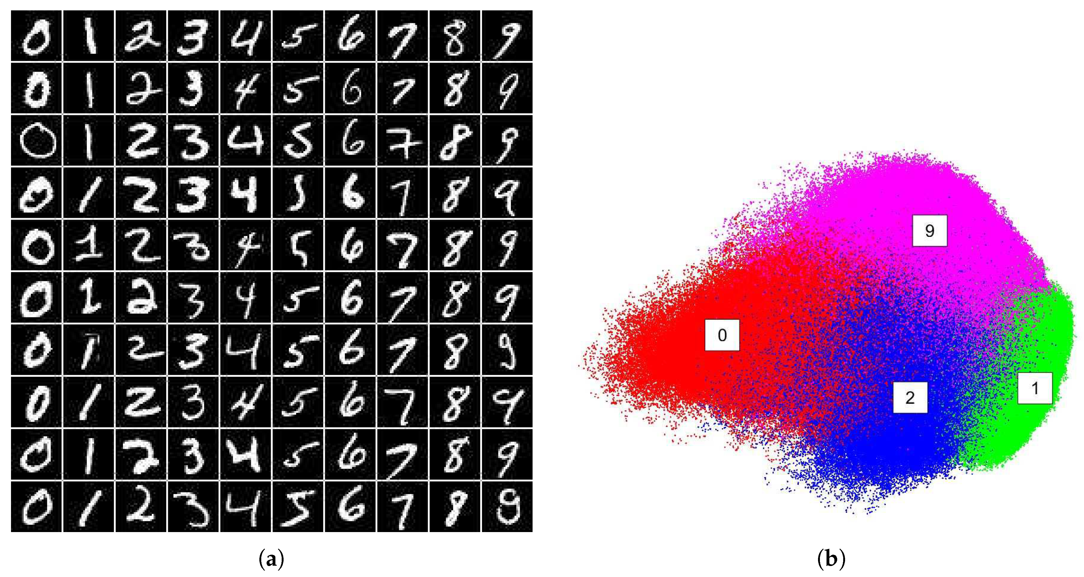
We used datasets from the UCI machine learning repository (http://archive.ics.uci.edu/ml/datasets.html), which are benchmark datasets in data clustering and classification tests. In addition, we used MNIST-8M dataset (http://leon.bottou.org/projects/infimnist) to verify the embedding ability of the proposed method on large-scale data. MNIST-8M contains 8 million 28 × 28 handwritten digit images labeled 0 to 9. MNIST-8M is built by elastic deformation of the original MNIST training set, which is a benchmark dataset for handwritten digits recognition. Figure 6a shows demos of MNIST-8M. Details of the employed datasets are shown in

Table 1. A summary of datasets.

Dataset	Size	Dimensions	Classes
Hayes	81	5	2
Iris	150	4	3
Wine	178	13	3
SVM Guide 4	300	10	6
Liver Disorders	345	6	2
Ionosphere	351	34	2
SVM Guide 2	391	20	3
Vowel	528	10	11
UCI Image	2310	19	7
SVM Guide 1	3089	4	2
Statlog Letter	10,500	16	26
MNIST-8M (Embedding only)	8,100,000	784	10

.

We compared the proposed method with four popular clustering methods on UCI datasets. The competing methods are listed as follows:

• Standard Nyström [10] (Nys), in which we randomly selected $m=k\times 10$ points as the training set.
• Random SVD Nyström [19] (RSNys), in which we used the default settings in Random SVD, i.e., over-sampling parameter $p=5$ and power parameter $q=2$.
• Normalized Cuts [5] (NCut), in which we used the default settings.
• Incremental k-means [20] (IncKM), in which we used the default settings.
• Our proposed method (IncSC), in which we used $D=4000$ Fastfood features for each data point and the $\beta$ convergence threshold ${ϵ}_{\beta }=k/10$ for all datasets.

In our UCI experiments, we used the default settings (if available) in each competing method. This is fair since we assumed that, in practice, users are blind to the ground truth labels and hence will run clustering with the default settings. We did not fine-tune our parameters in our experiments and fixed those in all tests.

4.2. Configurations and Evaluation Metrics

In our work, we adopted the Gaussian kernel, $\ker (x,y)=\exp (-\parallel x-y{\parallel }^2/2{\sigma }^2)$, in our clustering. In incremental clustering, there are two critical parameters that dominate the clustering results. The first is the number of desired clusters k and the second is the Gaussian parameter $\sigma$. Although self-tuning methods [21,22] were applied to select $\sigma$, it is still a challenging problem in searching for the optimal Gaussian scale parameter. We set the k as the ground truth number of classes. We further set the Gaussian scale parameter $\sigma$ as the average value of the square root of the distance sum.

It is noticeable that, in our works, we did not refer to any parameter fine-tuning technologies, such as cross validation. It is shown in many previous works that searching the optimal parameters via cross validation can significantly improve the clustering performance. In our works, however, we left the parameter searching blank and used the default settings of all competitors since: (a) it is still a fair competition with fixed parameters in all datasets; and (b) users are always blind to the ground truth labels and hence prefer to use the default configuration as the primary choice.

In our competitive tests, i.e., UCI datasets experiments, we employed clustering Accuracy, NMI and Eigenvector Relative Error to evaluate the performance of clustering results. On MNIST-8M and BSD500 tasks, we only show the embedding or segmentation results without further evaluation.

Accuracy is defined by

$$Acc=\frac{{\sum }_{i=1}^n\delta ({\widehat{c}}_i,map\left(c_i\right))}{n}$$

(13)

where ${\widehat{c}}_i$ is the ground truth label; $c_i$ is the derived label of the ith datum; $\delta (p,q)$ is the delta function where $\delta (p,q)=1$ if $p=q$ and $\delta (p,q)$=0 otherwise; and $map(·)$ is the best mapping function that matches the true labels and the derived ones. A larger Accuracy indicates a better clustering performance.

NMI is the second performance measure used in this paper. Let M and N be the random variables represented by the clustering labels generated from two competing methods. Denote $I(M,N)$ as the mutual information between M and N and $H\left(M\right)$ as the entropy of M. Then, NMI is defined as:

$$NMI(M,N)=\frac{I(M,N)}{\sqrt{H\left(M\right)H\left(N\right)}}$$

(14)

NMI ranges from 0 to 1 and takes the unitary value when two clustering labels are perfectly matched.

Eigenvector Relative Error (ERE) is used in our works to evaluate the eigenvector approximation accuracy. ERE is defined as

$$ERE=\frac{\parallel V-\tilde{V}{\parallel }_F}{{\parallel V\parallel }_F}$$

(15)

where V indicates the ground truth eigenvectors and $\tilde{V}$ is the approximated eigenvectors generated by our method. ${\parallel ·\parallel }_F$ means the Frobenius norm of a matrix.

4.3. Real-World Datasets

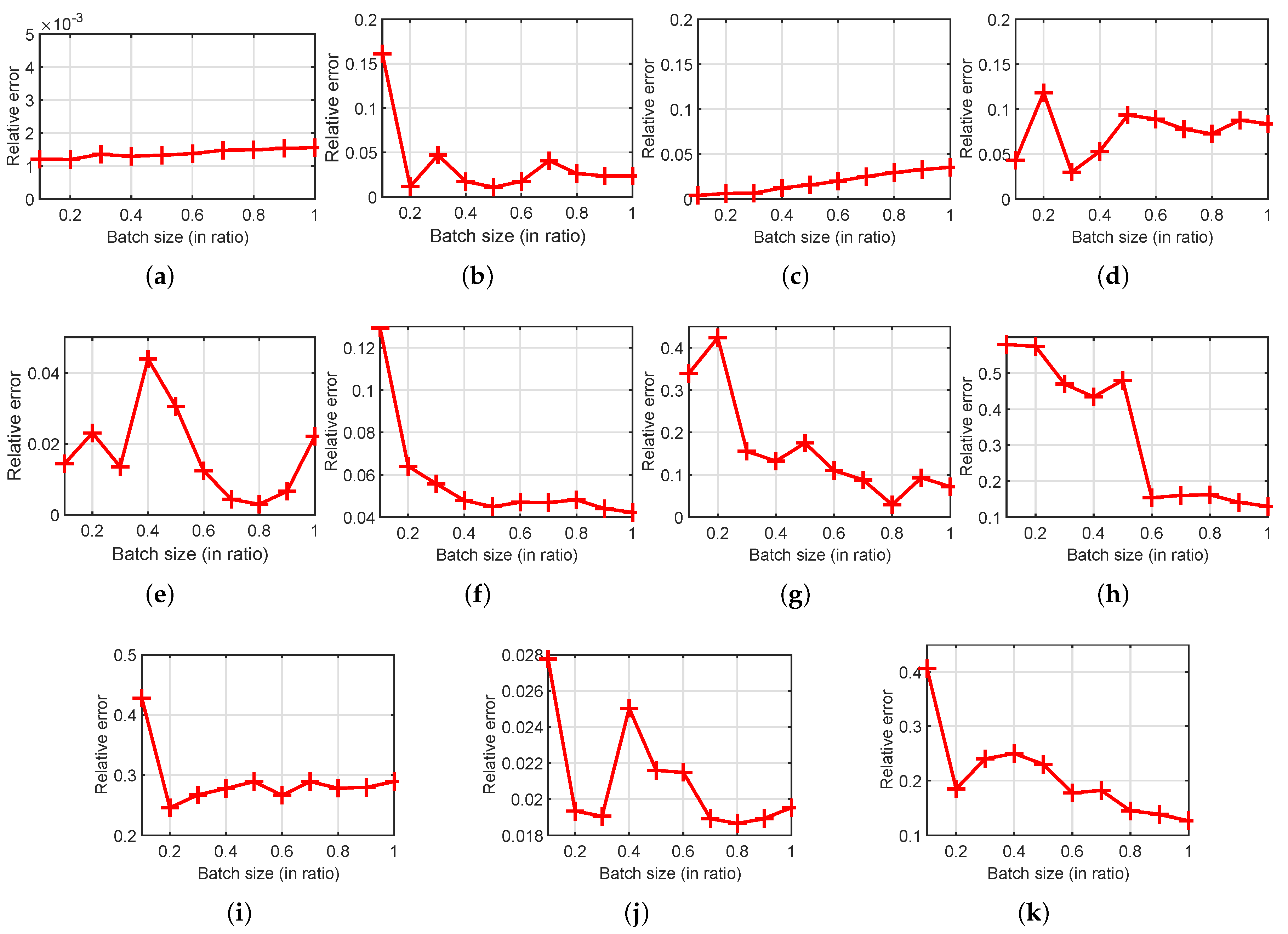
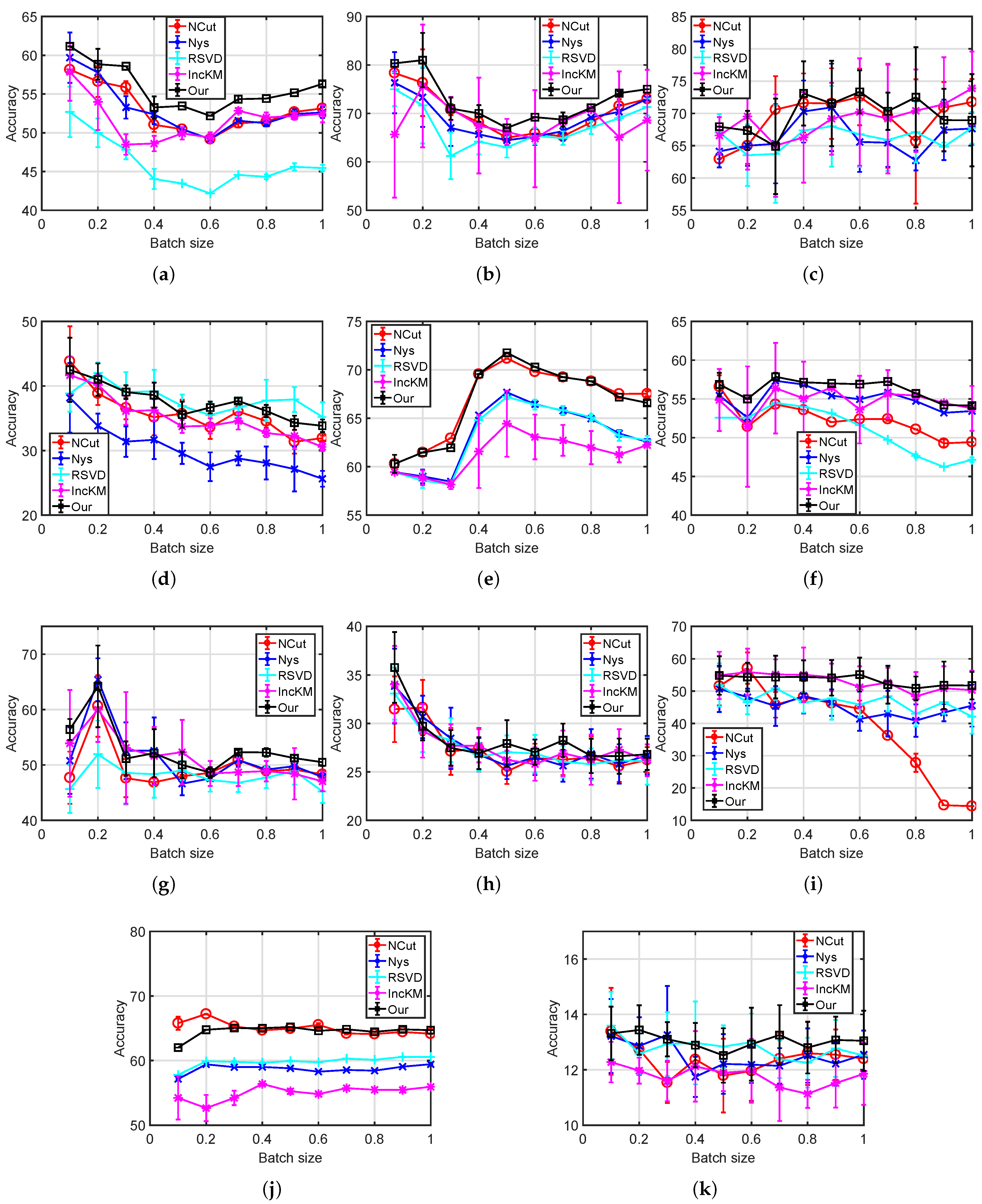
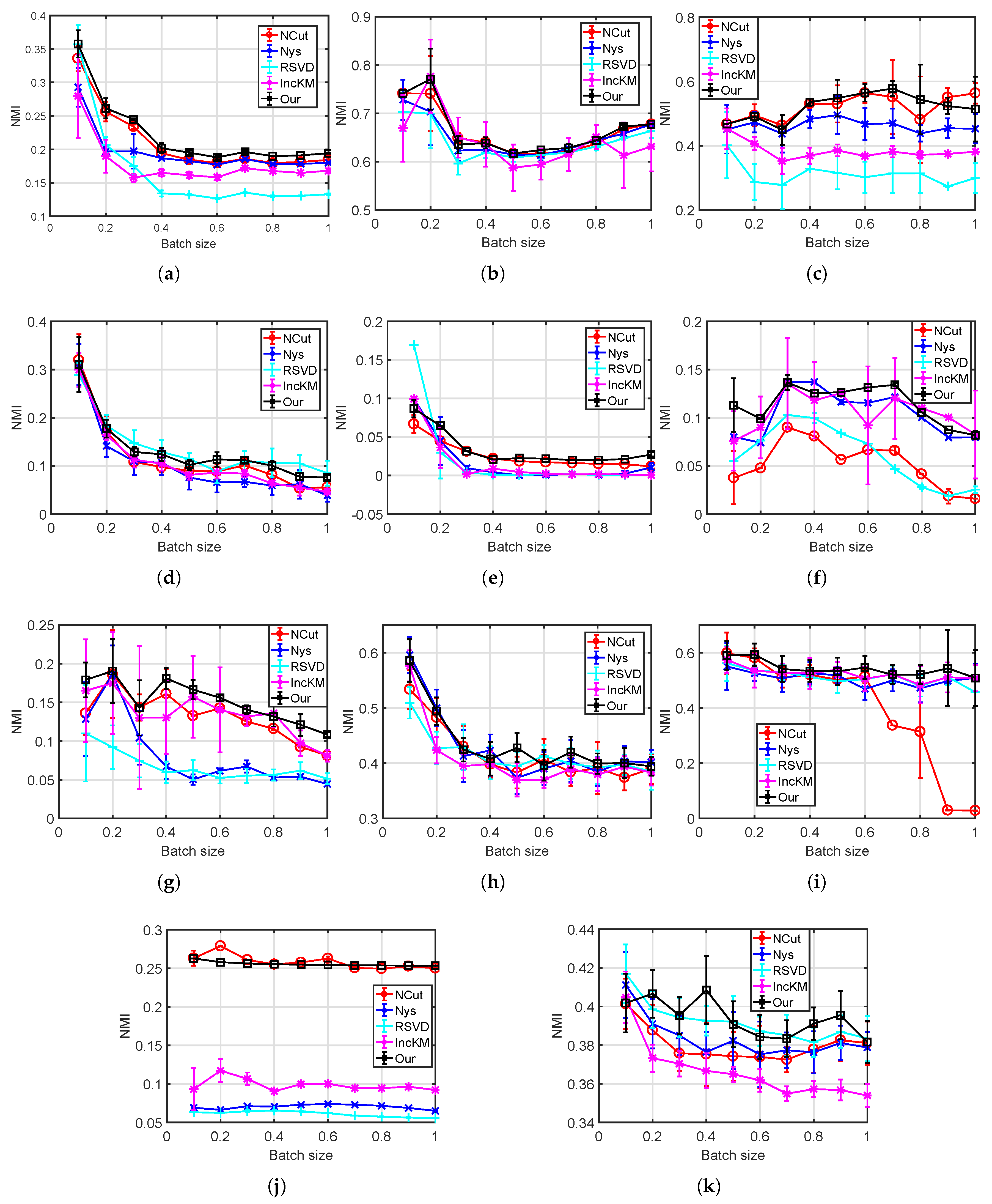
We tested our method on eleven datasets to verify the clustering performance. In this experiment, we first randomly separated one dataset into ten folds, and iteratively pushed one fold after another to the proposed method. At the i-th iteration, we calculated the clustering results as well as the eigenvector errors on the leading i folds and compared with that of the standard NCut, which performs as the ground truth values in this experiment. In Accuracy and NMI evaluation, we ran each competing methods 20 times and present the average value and the standard deviation. Figure 3 illustrates the eigenvector relative errors, Figure 4 shows the Accuracy in terms of various folds and Figure 5 refers to NMI.

In Figure 3, we can see that our method is able to improve its accuracy on eigenvector approximation as more data are seen. In Hayes, SVM Guide 4 and Liver Disorders, the ERE is stable through the whole dataset. Only on Wine, the ERE is slightly increased.

In Figure 4 and Figure 5, we can observe the following:

(1) Clustering performance of NCut is relatively promising in real-world datasets. On Liver Disorders and SVM Guide 1, NCut is among the top two methods in terms of Accuracy. Compared with traditional clustering methods such as k-means, the employment of kernel similarity and clustering in the kernel space ensures NCut can partition data points with non-convex structure, a case in which k-means may fail to work.

(2) As variants to NCut, the standard Nyström and Random SVD both are comparable to others. Both methods employ Nyström Gram matrix approximation to estimate the eigenvectors of K while RSVD uses random SVD for acceleration. RSVD obtains much lower Accuracy on Hayes and Nyström on SVM Guide 4. Both Nyström and RSVD need to sample training set from the current batch. If data distribution of the current batch is much different from that of the entire dataset, the sampled training set then may mislead to an incorrect partition.

(3) Clustering performance of incremental k-means is not stable. On SVM Guide 1 and most batches of Statlog Letter, incremental k-means obtains the lowest Accuracy. The standard k-means is known for its disadvantages in revealing the underlying structure of complicated datasets, such as the XOR problem. It is a challenging task for k-means-based method, including the incremental k-means, to partition on dataset with non-convex data distribution.

(4) The proposed incremental spectral clustering method obtains comparable, sometimes slightly better, results compared with other methods. Compared with Nyström-based methods, i.e., Nyström and RSVD, our method is able to recover from a bad sampling and provide robust clustering results regardless of arriving order. The clustering results, hence, are more stable than others.

4.4. Embeddings on Extremely Large Dataset

We verifyed our method on MNIST-8M dataset containing 8.1M data points. For visualization purpose, we only used digits 0, 1, 2 and 9, which result in a subset with about 3.3M data points. Due to the sheer shape, processing on MNIST-8M is difficult for the original spectral clustering or even the Nyström approximations.

To record the similarity matrix among the training set and the testing set, Nyström methods may require as large as a $(3.3\times {10}^6)\times m$ matrix storage, where m is the training size. If we use 100 points in the training set, or roughly 0.001% of the entire dataset, Nyström still requires almost 19.67 GB in the main memory with double (64 bit) format. Although we can release such memory burden by I/O processing, additional time costs are needed in this case. By contrast, our method is able to complete such embeddings in a memory-efficient way.

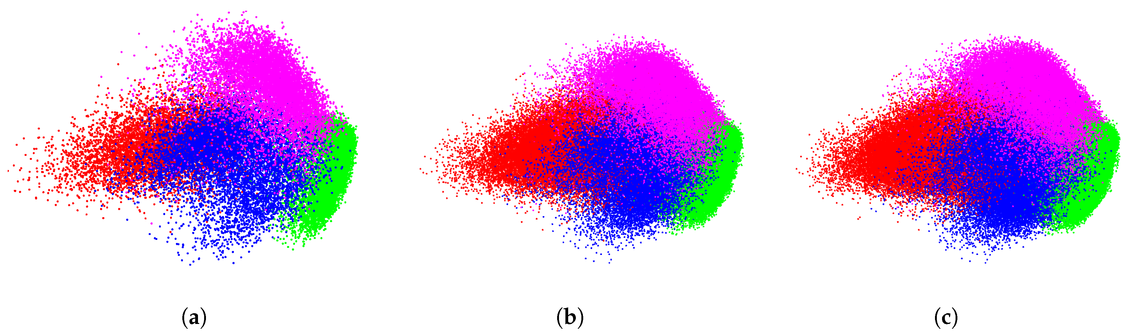
Our incremental spectral clustering is able to operate the huge dataset by streaming the data and processing one batch after another. Figure 6b shows our embedding results on the first two dimensions with $D=1200$. As can be seen, digits in embedding space are well structured. To further illustrate the performance of the proposed method in incremental embedding, we show the embeddings of the leading $[1\%,2\%,9\%]$ batches with a stride of 1%, or roughly 81K images per stride. Figure 7 shows the embeddings of digits 0, 1, 2 and 9 with various employed batch sizes.

4.5. Experiment on Incremental Image Segmentation

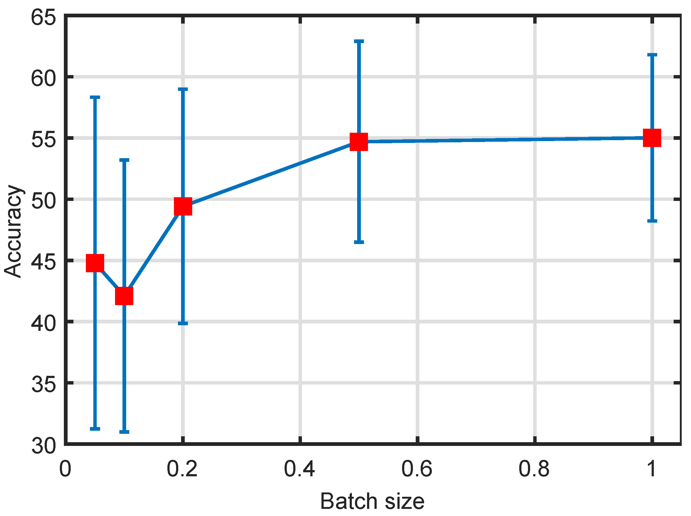
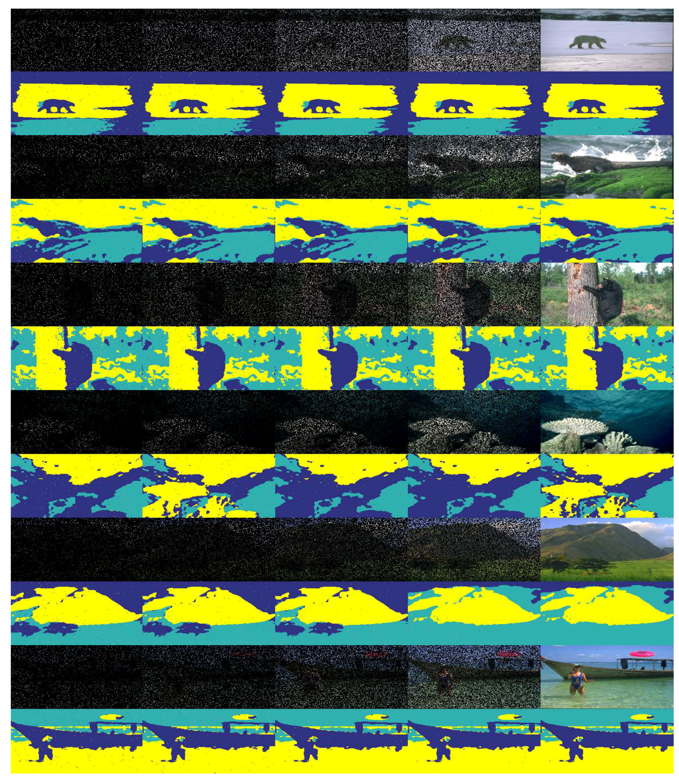
In this experiment, we tested our method on incremental image segmentation task. We used the test images from the Berkeley image segmentation dataset [23] (https://www2.eecs.berkeley.edu/Research/Projects/CS/vision/bsds/). Of each image, we loaded iteratively $[5\%,10\%,20\%,50\%,100\%]$ of the entire pixels as input and ran our incremental spectral clustering method on the partially (except the last test) observed image. To describe one pixel, similar to our previous works [6,24], we calculated a local color histogram, $h_b$, with a $2\times 2$ window centered at each pixel of an image. Thus, each pixel is featured by a descriptor of length $b\times 1$, where b is the number of bins in the color histogram $h_b$ and is fixed as $b=8$ in our test. We run our method on all 200 testing images and show the average Accuracy and its standard deviation values in Figure 8. Several segmentation results are shown in Figure 9.

In Figure 9, each subfigure consists of five columns representing input set size $[0.05,0.1,0.2,0.5,1]\times n$ pixels. We show in each column the partially-observed input image and its corresponding clustering results. In each partially-observed image, colored pixels indicate the observed ones and black ones mean unseen pixels. Our method iteratively loads the input pixels with growing volume and iteratively generates the clustering results. To extend the clustering results from the observed pixels to the unseen ones, we set the label of one unseen pixel the same as that of its nearest neighbour in the observed (hence labeled) pixels.

Our method, as shown in Figure 8 and Figure 9, improves the clustering results when more pixels are available. A similar approach can be found in Figure 3 where eigenvector errors are reduced when more data points are loaded. Ideally, the clustering approximation error of our method is determined by Fastfood approximation error when all batches are read from a pipeline. With the assumption that data points in the kernel space are linearly separable, which implies we are able to partition points by the leading eigenvectors of K, then our method is more likely to be convergent to the real partition.

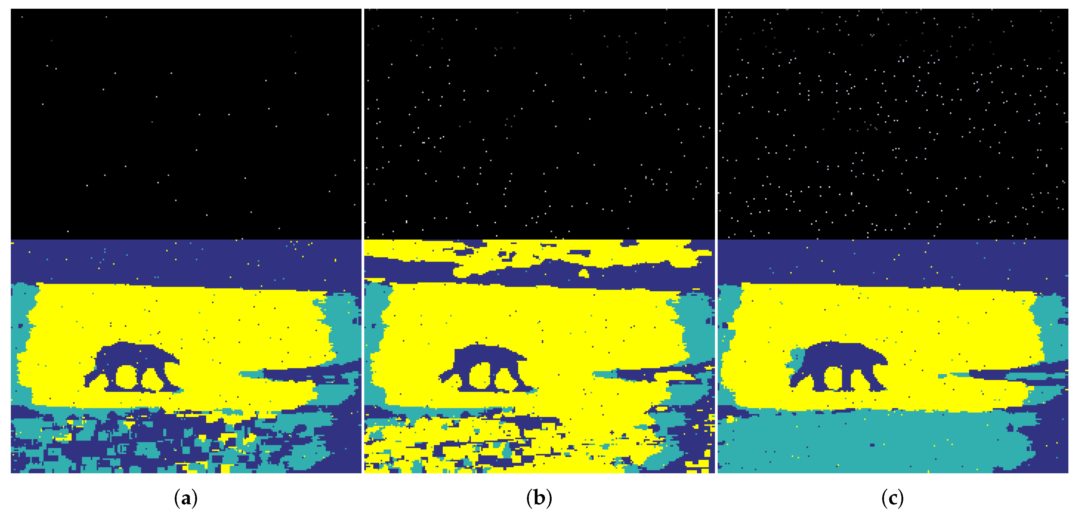
To further verify the performance of our method against very low batch sizes, we tested on BSD500 ID 100007 with batch size $[0.0001,0.0002,0.0005]\times n$, as shown in Figure 10. With very low batch size, e.g., batch size 0.01% in Figure 10a, our method attempts to reveal the structure of this image but many incorrect labels can be found. With more pixels seen, as shown in Figure 10b,c, the segmentation then is more accurate and close to the real partition.

5. Conclusions

In this paper, we propose an incremental image segmentation method based on Fastfood features. Our main idea consists of representing eigenvectors of the kernel matrix K in spectral clustering by that of G, where G is of fixed size and, as a result, can be upheld in main memory and process with G in real time. Compared with the standard spectral clustering, such as Normalized Cuts, our method is able to solve the eigensystem of K in an incremental fashion, indicating the ability to handle stream data which NCut may fail to do so. To obtain G, we represent data points in the kernel space, X, by Fastfood features and form our G by $G=X{X}^T$ and repeatedly update both G and its eigensystem with coming data from a pipeline. We then prove that we are able to solve the eigensystem of K by that of G and X. Thus, we approximate the eigenvectors of K, whose memory occupation increases quadratically, with a constant memory requirement and use the approximated eigenvectors to obtain the final partition. Our work is suitable for stream data clustering due to the one-shot process in our method. In addition, the proposed method is also able to handle large-scale data by loading data points from a pipeline. We verified our method on several real-world datasets and image segmentation tasks. Our method shows its ability in iteratively approximate the eigenvectors of K with more and more data seen. On clustering tasks, we compared our method with four competing methods and ours is comparable or slightly better than the competitors. We also tested on our embedding ability on MNIST-8M dataset, which consists of 8 million data points. We also applied our method on stream image segmentation tasks.

Our proposed method takes Fastfood features as its theoretical foundation to accurately approximate the kernel matrix K. Fastfood features belong to a family of methods entitled explicit feature mapping by which we can explicitly obtain the kernel mapped data point X. Approximation error of explicit feature mapping is shown related to the mapped dimension D, e.g., $O\left(\exp -D\right)$ of random Fourier features. By increasing D will improve the approximation accuracy but with the cost of additional time and memory costs. A good balance between efficiency and accuracy is a task-driven problem and there is not a general solution. In addition, for extremely large-scale datasets, we need to build a parallel-computing-friendly variant of our method. We did not employ parameter optimization in our experiments. Parameter fine-tuning, e.g., via cross validation, is shown to significantly improve clustering performance. We keep the study of an efficient method in determining our parameters as one of our further works.

References

- Yin, S.; Gong, M.; Gong, M. Unsupervised hierarchical image segmentation through fuzzy entropy maximization. Pattern Recognit. 2017, 68, 245–259. [Google Scholar] [CrossRef]
- Gong, M.; Qian, Y.; Li, C. Integrated Foreground Segmentation and Boundary Matting for Live Videos. IEEE Trans. Image Process. 2015, 24, 1356–1370. [Google Scholar] [CrossRef] [PubMed]
- Chen, P.; Zhang, X.; Chen, X.; Liu, M. Path Planning Strategy for Vehicle Navigation Based on User Habits. Appl. Sci. 2018, 8, 407. [Google Scholar] [CrossRef]
- Li, F.; Li, T.; Wang, H.; Jiang, Y. A Temperature Sensor Clustering Method for Thermal Error Modeling of Heavy Milling Machine Tools. Appl. Sci. 2017, 7, 82. [Google Scholar] [CrossRef]
- Shi, J.; Malik, J. Normalized cuts and image segmentation. IEEE Trans. Pattern Anal. Mach. Intell. 2000, 22, 888–905. [Google Scholar] [Green Version]
- He, L.; Zhang, H. Iterative Ensemble Normalized Cuts. Pattern Recognit. 2016, 10, 111–123. [Google Scholar] [CrossRef]
- Ning, H.; Xu, W.; Chi, Y.; Gong, Y.; Huang, T.S. Incremental spectral clustering by efficiently updating the eigen-system. Pattern Recognit. 2010, 43, 113–127. [Google Scholar] [CrossRef]
- Dhanjal, C.; Gaudel, R.; Clémençon, S. Efficient eigen-updating for spectral graph clustering. Neurocomputing 2014, 131, 440–452. [Google Scholar] [CrossRef] [Green Version]
- Le Quoc, V.; Sarlos, T.; Smola, A.J. Fastfood: Approximate Kernel Expansions in Loglinear Time. arXiv, 2013; arXiv:1408.3060. [Google Scholar]
- Williams, C.; Seeger, M. Using the nyström method to speed up kernel machines. In Proceedings of the 14th Annual Conference on Neural Information Processing Systems, Vancouver, BC, Canada, 3–8 December 2001; pp. 682–688. [Google Scholar]
- Fowlkes, C.; Belongie, S.; Chung, F.; Malik, J. Spectral grouping using the Nystrom method. IEEE Trans. Pattern Anal. Mach. Intell. 2004, 26, 214–225. [Google Scholar] [CrossRef] [PubMed]
- Wang, S.; Zhang, Z. Improving Cur Matrix Decomposition and the Nyström Approximation Via Adaptive Sampling. J. Mach. Learn. Res. 2013, 14, 2729–2769. [Google Scholar]
- Boutsidis, C.; Drineas, P.; Magdon-Ismail, M. Near-Optimal Column-Based Matrix Reconstruction. SIAM J. Comput. 2014, 43, 687–717. [Google Scholar] [CrossRef] [Green Version]
- Wen, J.; Zhou, Z.; Wang, J.; Tang, X.; Mo, Q. A sharp condition for exact support recovery with orthogonal matching pursuit. IEEE Trans. Signal Process. 2017, 65, 1370–1382. [Google Scholar] [CrossRef]
- Wen, J.; Wang, J.; Zhang, Q. Nearly optimal bounds for orthogonal least squares. IEEE Trans. Signal Process. 2017, 65, 5347–5356. [Google Scholar] [CrossRef]
- Rahimi, A.; Recht, B. Random features for large-scale kernel machines. In Proceedings of the Advances in Neural Information Processing Systems, Vancouver, BC, Canada, 3–6 December 2007; pp. 1177–1184. [Google Scholar]
- Sutherland, D.J.; Schneider, J. On the error of random Fourier features. arXiv, 2015; arXiv:1506.02785. [Google Scholar]
- Lin, F.; Cohen, W.W. Power iteration clustering. In Proceedings of the International Conference on Machine Learning, Haifa, Israel, 21–24 June 2010; pp. 655–662. [Google Scholar]
- Li, M.; Bi, W.; Kwok, J.T.; Lu, B.-L. Large-scale Nyström kernel matrix approximation using randomized SVD. IEEE Trans. Neural Netw. Learn. Syst. 2015, 26, 152–164. [Google Scholar] [PubMed]
- Aaron, B.; Dan, E.T.; Rishe, N.D.; Kandel, A. Dynamic Incremental K-means Clustering. In Proceedings of the International Conference on Computational Science and Computational Intelligence, Las Vegas, NV, USA, 10–13 March 2014; pp. 308–313. [Google Scholar]
- Zelnik-Manor, L.; Perona, P. Self-Tuning Spectral Clustering. In Proceedings of the Advances in Neural Information Processing Systems, Vancouver, BC, Canada, 13–16 December 2004; pp. 1601–1608. [Google Scholar]
- Yiming, Q.; Gong, M.; Cheng, L. STOCS: An Efficient Self-Tuning Multiclass Classification Approach. In Proceedings of the Canadian Conference on Artificial Intelligence, Halifax, NS, Canada, 2–5 June 2015; pp. 291–306. [Google Scholar]
- Martin, D.; Fowlkes, C.; Tal, D.; Malik, J. A database of human segmented natural images and its application to evaluating segmentation algorithms and measuring ecological statistics. In Proceedings of the Eighth IEEE International Conference on Computer Vision, Vancouver, BC, Canada, 7–14 July 2001; pp. 416–423. [Google Scholar]
- He, L.; Zhang, H. Kernel K-means Sampling for Nystrom Approximation. IEEE Trans. Image Process. 2018, 27, 2108–2120. [Google Scholar] [CrossRef] [PubMed]
Figure 1.
A demonstration of stream data processing. A clustering method, such as spectral clustering, will receive iteratively a new batch of data from a data pipeline and process on each batch in real time. Finally, this clustering method is expected to obtain the final partition of the entire dataset according to batch-clustering-results.
Figure 2.
Framework of the proposed method.
Figure 3.
Eigenvector approximation relative errors: (a) Hayes; (b) Iris; (c) Wine; (d) SVM Guide 4; (e) Liver Disorders; (f) Ionosphere; (g) SVM Guide 2; (h) Vowel; (i) UCI Image; and (j) SVM Guide 1; and (k) Statlog Letter.
Figure 4.
Clustering results on several real-world datasets, Accuracy: (a) Hayes; (b) Iris; (c) Wine; (d) SVM Guide 4; (e) Liver Disorders; (f) Ionosphere; (g) SVM Guide 2; (h) Vowel; (i) UCI Image; (j) SVM Guide 1; and (k) Statlog Letter.
Figure 5.
Clustering results on several real-world datasets, NMI: (a) Hayes; (b) Iris; (c) Wine; (d) SVM Guide 4; (e) Liver Disorders; (f) Ionosphere; (g) SVM Guide 2; (h) Vowel; (i) UCI Image; (j) SVM Guide 1; and (k) Statlog Letter.
Figure 6.
Demo data of MNIST-8M dataset and embeddings by the proposed method: (a) demos of MNIST-8M; and (b) embeddings of digits 0, 1, 2 and 9 by our method.
Figure 7.
Embeddings of MNIST-8M dataset with the leading batches: (a–c) Embeddings of the digits 0, 1, 2 and 9 with the leading batches . The sheer volume of MNIST-8M prevents the application of most clustering methods. Our incremental spectral clustering, by contrast, is able to handle data in a stream fashion, i.e., read and process data from a pipeline with neither re-visiting historical data nor huge (thus impossible in practice) storage in the main memory.
Figure 8.
Image incremental segmentation results, Accuracy. Different stacks correspond to different image IDs and of one stack the five different bars show the Accuracy of different observed data sizes.
Figure 9.
A demonstration of the incremental image segmentation results. Every two rows correspond to one image. Top to bottom: ID 100007, ID 103078, ID 100039, ID 101027, ID 28083 and ID 81066. Pixels of each image are read from a pipeline and our method processes the current batch in real time without any re-visiting to previous pixels. Different columns correspond to different observed pixel sizes ranging from 5% (left) to 100% (right). The upper row of each subfigure shows the observed pixels where black pixels indicate the unseen ones. The lower row displays the corresponding segmentation results.
Figure 10.
Segmentation with very low batch sizes: (a) Batch size 0.01%; (b) Batch size 0.02%; and (c) Batch size 0.05%.