Numerical Study of Dynamic Properties of Fractional Viscoplasticity Model

Abstract

The fractional viscoplasticity (FV) concept combines the Perzyna type viscoplastic model and fractional calculus. This formulation includes: (i) rate-dependence; (ii) plastic anisotropy; (iii) non-normality; (iv) directional viscosity; (v) implicit/time non-locality; and (vi) explicit/stress-fractional non-locality. This paper presents a comprehensive analysis of the above mentioned FV properties, together with a detailed discussion on a general 3D numerical implementation for the explicit time integration scheme.

1. Introduction

In search of a generalization of existing models describing experimentally observed phenomena, the concept of fractional calculus [1,2] emerged as a tool that in the recent years became widely applied. Among the areas in which this theory has found application, it is worth mentioning mechanics where one can distinguish: (i) time-fractional models; (ii) space-fractional models; and (iii) stress-fractional models. For example, in [3], the time-fractional model was used to describe the time-dependent mechanical property evolution in ductile metals. The fractional oscillators were analyzed in [4], whereas the heat and mass transfer analysis in the framework of fractional calculus was presented in [5,6]. Furthermore, the analysis and modeling of turbulent flow in a porous medium [7], fluid transport induced by the osmotic pressure of glucose and albumin [8], wave propagation in the viscoelastic material [9], non-local boundary value problem [10], and evolution for the damage variable for hyperelastic materials [11] with an application of time-fractional derivative suggests great versatility of this approach. On the other hand, the space-fractional models are successfully used in mechanics to describe the deformation of a harmonic oscillator [12], deformation of an infinite bar subjected to a self-equilibrated load distribution [13], modeling plane strain and plane stress elasticity [14], Euler–Bernoulli beam [15], Darcy’s flow in porous media [16] and fractional strain formulation [17]. Finally, the stress-fractional models [18,19] and their finite element implementations were used to study the granular soils under drained cyclic loading [20], and monotonic triaxial compression [21]. Concluding, one should emphasize that regardless of the specific formulation, the fractional operators have one common feature, namely, the ‘change’ of a selected variable is based on integration over a closed interval, thus extending the definition of integer order derivative (defined in a point) and simultaneously introducing a non-locality in a given space.

It is commonly accepted that the Theory of Thermo-Viscoplasticity (TTV), which plays a central role in the following considerations, began with the publication of Perzyna [22], which, until the present day, serves a basis for many efforts in linking experimental and numerical results for different types of materials. The main results of this theory were discussed in a great number of papers that focused on phenomena such as propagation of mechanical and thermal waves [23,24], viscosity controlled by material parameter [25,26], dispersion [26], or implicit non-locality in the time variable [27]. Nonetheless, the classical TTV formulation does not include directional viscosity, and to include the non-normality extension needs, as all classical plasticity theories, postulation of an additional potential, which is not straightforward and causes the increase of material parameters. Furthermore, the same concern is relevant to the plastic anisotropy effects in terms of the original Perzyna model; to include this effect additional variables and evolution equations for them are needed to be postulated. This limitations were resolved by the generalization of the Perzyna formulation by definition of the fractional flow rule, first proposed in [18] and later developed in [19,28,29,30].

The implementation of the fractional plastic (rate independent) rule, for the Huber-Mises-Hencky (HMH) yield criterion, in the framework of implicit and explicit procedures and with examples on material point level, was presented in [28]. This was further developed in the subsequent article [29] to any smooth and convex yield criterion but still focusing on rate independent plastic flow. Concluding, in both these articles the non-locality in the stress state was present, however the implicit time non-locality common for the viscoplastic flow was not included in them.

This paper extends the concept of FV, which was first reported in [18], for the Initial Boundary Value Problem (IBVP), and provides a detailed discussion of the model material parameters. The parametric study includes the influence of the overstress power and the relaxation time (which is understood as implicit length scale parameter, as mentioned in [27]) on the dynamic properties of the FV model. Moreover, additional fractional material parameters, which induce the directional viscosity, the non-associative, and the anisotropic plastic flow, were also discussed.

2. Fractional Viscoplasticity

2.1. Remarks on Fractional Calculus

Fractional calculus (FC) introduces a new, universal method for calculating the intensity of changes of various quantities in mathematical models describing experimentally observed phenomena. FC implies a generalization of integer order derivatives, by fractional derivatives (FD). The selection of the FD definition (from an infinite number) can use a type of material as a criterion to obtain the best fitting of the constitutive model to a given experimental evidence. All definitions of the FD have a common property, namely they include summation over an interval abandoning the integer order derivative definition given at a single point; therefore they are called non-local. The classical derivative can be regarded a special case of the FD when its order becomes integer.

In order to explain the FD concept, let us consider a generalized fractional differential operator $B_P^{\alpha }$ as a composition of fractional integral $K_P^{\alpha }$ with classical integer (n-th) differential operator [31]

$$B_P^{\alpha }=K_P^{n-\alpha }\circ \frac{d^n}{d{t}^n},$$

(1)

where $\alpha$ is the order of the derivative, $n=⎣\alpha ⎦+1$, $⎣·⎦$ denotes the floor function, P is a parameter set (described below) and ∘ denotes the composition operator. $B_P^{\alpha }$ is referred to as the fractional differential operator B (B-op) of order $\alpha$ and p-set P, and analogously $K_P^{\alpha }$ identifies the K (K-op) fractional integer operator of order $\alpha$ and p-set P.

The definition of K for the parameter set $P=〈a,t,b,p,q〉$ can be given as

$$\left(K_P^{\alpha }f\right)\left(t\right)=p{\int }_a^t{k}_{\alpha }(t,\tau )f\left(\tau \right)d\tau +q{\int }_t^b{k}_{\alpha }(\tau ,t)f\left(\tau \right)d\tau ,$$

(2)

where $t\in \left[a,b\right]$ and $a<t<b$, $p,q$ are real numbers, and $k_{\alpha }(t,\tau )$ is a kernel that depends on the order of the derivative $\alpha$. It can be shown that if $k_{\alpha }$ is a difference kernel, i.e., $k_{\alpha }(t,\tau )=k_{\alpha }(t-\tau )$ and $k_{\alpha }\in L_1\left(\left[0,b-a\right]\right)$ then $L_1\left(\left[b,a\right]\right)\to L_1\left(\left[b,a\right]\right)$ is well defined, bounded and linear. For explicit definition, the special form of the kernel function can be assumed

$$k_{\alpha }(t-\tau )=\frac{1}{\mathsf{\Gamma }\left(\alpha \right)}{\left(t-\tau \right)}^{\alpha -1},$$

(3)

then for $P=〈a,t,b,1,0〉$

$$\left(K_P^{\alpha }f\right)\left(t\right)=\frac{1}{\mathsf{\Gamma }\left(\alpha \right)}{\int }_a^t{(t-\tau )}^{\alpha -1}f\left(\tau \right)d\tau =\left({}_a{I}_t^{\alpha }f\right)\left(t\right),$$

(4)

is obtained or, if $P=〈a,t,b,0,1〉$ then

$$\left(K_P^{\alpha }f\right)\left(t\right)=\frac{1}{\mathsf{\Gamma }\left(\alpha \right)}{\int }_t^b{(\tau -t)}^{\alpha -1}f\left(\tau \right)d\tau =\left({}_t{I}_b^{\alpha }f\right)\left(t\right),$$

(5)

where $\mathsf{\Gamma }$ is the Euler gamma function. Equations (4) and (5) describe the left and right Riemann-Liouville fractional integrals of the order $\alpha$, respectively. The application of these operators in Equation (1) leads to the following fractional derivative definitions:

$$\left(B_P^{\alpha }\right)f\left(t\right)={}_a^C{D}_t^{\alpha }f\left(t\right)=\frac{1}{\mathsf{\Gamma }(n-\alpha )}{\int }_a^t\frac{f^{\left(n\right)}\left(\tau \right)}{{(t-\tau )}^{\alpha -n+1}}d\tau ,$$

(6)

for $t>a$, and

$$-\left(B_P^{\alpha }\right)f\left(t\right)={}_t^C{D}_b^{\alpha }f\left(t\right)=\frac{{(-1)}^n}{\mathsf{\Gamma }(n-\alpha )}{\int }_t^b\frac{f^{\left(n\right)}\left(\tau \right)}{{(\tau -t)}^{\alpha -n+1}}d\tau ,$$

(7)

for $t<b$. The FD operators ${}_a^C{D}_t^{\alpha }f\left(t\right)$ and ${}_t^C{D}_b^{\alpha }f\left(t\right)$ are known as the left- and right-sided Caupto fractional integrals.

Finally, for the purpose of further definition of the FV, the Riesz-Caputo (RC) derivative can be expressed as a linear combination of previously given left and right Caputo derivatives

$${}_a^{RC}{D}_b^{\alpha }f\left(t\right)=\frac{1}{2}\left({}_a^C{D}_t^{\alpha }f\left(t\right)+{(-1)}^n{}_t^C{D}_b^{\alpha }f\left(t\right)\right).$$

(8)

It can be shown that for the RC derivative the fundamental property of integer order derivatives is preserved, that is, the derivative of a constant is zero.

2.2. Basic Concepts

In the following section Voigt notation is applied, thus the second rank tensors are ordered as ($6\times 1$ column matrix)

$$\mathbf{t}={\left(t_{11}{t}_{22}{t}_{33}{t}_{23}{t}_{13}{t}_{12}\right)}^{\mathrm{T}}={\left(t_1{t}_2{t}_3{t}_4{t}_5{t}_6\right)}^{\mathrm{T}},$$

(9)

whereas the fourth order tensors are represented by $6\times 6$ matrices ordered in accordance with the rule used in Equation (9).

Deformation assumes the additive decomposition of total strain, therefore

$$\epsilon ={\epsilon }^e+{\epsilon }^{vp},$$

(10)

or in a rate form

$$\dot{\epsilon }={\dot{\epsilon }}^e+{\dot{\epsilon }}^{vp},$$

(11)

where is the total strain, ${\epsilon }^e$ is the elastic strain and ${\epsilon }^{vp}$ is the viscoplastic strain. Next, due to thermodynamic restrictions, the elastic strain is related to elastic stress through Hooke’s law

$${\sigma }^e={\mathcal{L}}^e{\epsilon }^e,$$

(12)

where σ^e denotes the Cauchy stress tensor and ${\mathcal{L}}^e$ denotes the elastic constitutive tensor. The rate of viscoplastic strain is analogous to the classical viscoplastic definition, namely

$${\dot{\epsilon }}^{vp}=\Lambda \mathbf{p},$$

(13)

where $\Lambda$ is a scalar multiplier and $\mathbf{p}$ is the second order unit tensor which governs the direction of viscoplastic flow. As the $\mathbf{p}$ tensor is normalized, the magnitude of ${\dot{\epsilon }}^{vp}$ depends solely on the $\Lambda$ parameter.

Following the concept introduced by Perzyna [22], this parameter is expressed as

$$\Lambda =\gamma 〈\mathsf{\Phi }\left(F\right)〉,$$

(14)

where $\gamma =\frac{1}{T_m}$ is the viscosity parameter, $\mathsf{\Phi }$ is the overstress function that depends on the rate-independent yield surface F, and $〈·〉$ is Macaulay brackets. It is well-known that $\gamma$ introduces implicit time non-locality in the viscoplastic model [27]. Furthermore, the function $\mathsf{\Phi }$ has the following form

$$\mathsf{\Phi }\left(F\right)=F^{m_{vp}}={\left(\frac{\sqrt{J_2}}{\kappa }-1\right)}^{m_{vp}},$$

(15)

where $\sqrt{J_2}$ denotes the second invariant of stress deviator and $\kappa$ is the static yield stress in simple shear.

Finally, the remaining object needed to be defined is the tensor $\mathbf{p}$. In this place, the difference between the classical theory of viscoplasticity and the new approach is most evident. Let us recall, that in the classical formulation the direction of yield is normal to yield surface and $\mathbf{p}$ can be written as

$$\mathbf{p}=\frac{\partial F}{\partial }{\left(\left|\left|\frac{\partial F}{\partial }\right|\right|\right)}^{-1}.$$

(16)

It is also well known, that Equations (16) and (15) indicate that the viscoplastic strain is coaxial with the deviatoric stress tensor (associated flow). As a result, the volume change can occur in the range of elastic deformations only. For modern materials such as metal-matrix composites, this assumption is no longer valid. Therefore, the constitutive model should be modified to capture this phenomenon.

The fractional approach assumes the application of the RC operator to $\mathbf{p}$ definition [18]. In such a case, Equation (16) is generalized to the form

$$\mathbf{p}=D^{\alpha }F{\left|\left|D^{\alpha }F\right|\right|}^{-1},$$

(17)

where $D^{\alpha }$ stands for the RC operator (see Equation (8)). It is worth noting that the proposed formulation of $\mathbf{p}$ introduces the anisotropy of viscoplastic flow and furthermore (due to non-associativity) develops a tool to control the volume change in the plastic range of material behaviour [18]. Another essential remark is that Equation (17) introduces explicit stress-fractional non-locality in the overall model. It is important that the thermodynamic restrictions are formulated in a standard manner, and because of complicated structure of Equation (17) they are checked incrementally in the numerical procedure (see [29] for a detailed discussion).

3. Implementation

Introduction of the three-dimensional fractional viscoplastic model requires a numerical procedure that governs the solution. Since our considerations are focused on extreme dynamic processes, the explicit time integration was chosen for finite element method. Therefore, the ABAQUS/Explicit code was utilized together with the user subroutine VUMAT. The critical steps of the implementation are presented below.

In the first step, Hooke’s law is written as

$$\left\{\begin{array}{c}{\sigma }_{11}\\ {\sigma }_{22}\\ {\sigma }_{33}\\ {\sigma }_{23}\\ {\sigma }_{13}\\ {\sigma }_{12}\end{array}\right\}=\left(\begin{array}{cccccc}2G+\lambda & \lambda & \lambda & 0& 0& 0\\ \lambda & 2G+\lambda & \lambda & 0& 0& 0\\ \lambda & \lambda & 2G+\lambda & 0& 0& 0\\ 0& 0& 0& G& 0& 0\\ 0& 0& 0& 0& G& 0\\ 0& 0& 0& 0& 0& G\end{array}\right)\left\{\begin{array}{c}{\epsilon }_{11}\\ {\epsilon }_{22}\\ {\epsilon }_{33}\\ 2{\epsilon }_{23}\\ 2{\epsilon }_{13}\\ 2{\epsilon }_{12}\end{array}\right\},$$

(18)

where $G=E/2(1+\nu )$ and $\lambda =E\nu /(1+\nu )(1-2\nu )$ are elastic constants and E and $\nu$ denote Young’s modulus and Poisson’s ratio, respectively. Next, because of application of the HMH yield criterion, the yield function in a matrix form is as follows

$$F\left(\right)={\left\{\begin{array}{c}{\sigma }_{11}\\ {\sigma }_{22}\\ {\sigma }_{33}\\ {\sigma }_{23}\\ {\sigma }_{13}\\ {\sigma }_{12}\end{array}\right\}}^T\left(\begin{array}{cccccc}1& -\frac{1}{2}& -\frac{1}{2}& 0& 0& 0\\ -\frac{1}{2}& 1& -\frac{1}{2}& 0& 0& 0\\ -\frac{1}{2}& -\frac{1}{2}& 1& 0& 0& 0\\ 0& 0& 0& 3& 0& 0\\ 0& 0& 0& 0& 3& 0\\ 0& 0& 0& 0& 0& 3\end{array}\right)\left\{\begin{array}{c}{\sigma }_{11}\\ {\sigma }_{22}\\ {\sigma }_{33}\\ {\sigma }_{23}\\ {\sigma }_{13}\\ {\sigma }_{12}\end{array}\right\}-3{\kappa }^2=0.$$

(19)

Afterwards, the increment of viscoplastic strain (see Equations (13) and (17)) can be written in the form

$$\Delta {\epsilon }^{vp}=\Delta t\Lambda \mathbf{p}=\Delta t\Lambda \frac{{\left\{\begin{array}{cccccc}{\underset{{\sigma }_{11}}{D}}^{\alpha }F& {\underset{{\sigma }_{22}}{D}}^{\alpha }F& {\underset{{\sigma }_{33}}{D}}^{\alpha }F& {\underset{{\sigma }_{23}}{D}}^{\alpha }F& {\underset{{\sigma }_{13}}{D}}^{\alpha }F& {\underset{{\sigma }_{12}}{D}}^{\alpha }F\end{array}\right\}}^T}{\left|\left|D^{\alpha }F\right|\right|},$$

(20)

where (cf. [28])

$$\left\{\begin{array}{c}{p}_{11}\\ p_{22}\\ p_{33}\\ p_{23}\\ p_{13}\\ p_{12}\end{array}\right\}=\left(\begin{array}{cccccc}{k}_{\left(11\right)}^M& -\frac{1}{2}{k}_{\left(11\right)}^M& -\frac{1}{2}{k}_{\left(11\right)}^M& 0& 0& 0\\ -\frac{1}{2}{k}_{\left(22\right)}^M& k_{\left(22\right)}^M& -\frac{1}{2}{k}_{\left(22\right)}^M& 0& 0& 0\\ -\frac{1}{2}{k}_{\left(33\right)}^M& -\frac{1}{2}{k}_{\left(33\right)}^M& k_{\left(33\right)}^M& 0& 0& 0\\ 0& 0& 0& 3k_{\left(23\right)}^M& 0& 0\\ 0& 0& 0& 0& 3k_{\left(13\right)}^M& 0\\ 0& 0& 0& 0& 0& 3k_{\left(12\right)}^M\end{array}\right)\left\{\begin{array}{c}{\sigma }_{11}\\ {\sigma }_{22}\\ {\sigma }_{33}\\ {\sigma }_{23}\\ {\sigma }_{13}\\ {\sigma }_{12}\end{array}\right\}+\left\{\begin{array}{c}{k}_{\left(11\right)}^Q\\ k_{\left(22\right)}^Q\\ k_{\left(33\right)}^Q\\ 3k_{\left(23\right)}^Q\\ 3k_{\left(13\right)}^Q\\ 3k_{\left(12\right)}^Q\end{array}\right\}.$$

(21)

Symbols in Equation (21) denotes

$$k_{\left(ij\right)}^M=\frac{\mathsf{\Gamma }\left(2\right)}{\mathsf{\Gamma }(2-\alpha )}\left[{\left({\Delta }_{\left(ij\right)}^L\right)}^{1-\alpha }+{\left({\Delta }_{\left(ij\right)}^R\right)}^{1-\alpha }\right],$$

(22)

$$k_{\left(ij\right)}^Q=\left(\frac{\mathsf{\Gamma }\left(2\right)}{\mathsf{\Gamma }(2-\alpha )}-\frac{1}{2}\frac{\mathsf{\Gamma }\left(3\right)}{\mathsf{\Gamma }(3-\alpha )}\right)\left[{\left({\Delta }_{\left(ij\right)}^R\right)}^{2-\alpha }-{\left({\Delta }_{\left(ij\right)}^L\right)}^{2-\alpha }\right],$$

(23)

$${\Delta }^{\mathbf{L}}={\left(\begin{array}{cccccc}{\Delta }_{\left(11\right)}^L& {\Delta }_{\left(22\right)}^L& {\Delta }_{\left(33\right)}^L& {\Delta }_{\left(23\right)}^L& {\Delta }_{\left(13\right)}^L& {\Delta }_{\left(12\right)}^L\end{array}\right)}^T,$$

(24)

and

$${\Delta }^{\mathbf{R}}={\left(\begin{array}{cccccc}{\Delta }_{\left(11\right)}^R& {\Delta }_{\left(22\right)}^R& {\Delta }_{\left(33\right)}^R& {\Delta }_{\left(23\right)}^R& {\Delta }_{\left(13\right)}^R& {\Delta }_{\left(12\right)}^R\end{array}\right)}^T,$$

(25)

where

$$a_{\left(ij\right)}={\sigma }_{ij}-{\Delta }_{\left(ij\right)}^L,b_{\left(ij\right)}={\sigma }_{ij}+{\Delta }_{\left(ij\right)}^R.$$

(26)

Terminals $a_{\left(ij\right)},b_{\left(ij\right)}$ are needed to define the partial fractional derivatives in Equation (17) that enforce the directional nature of the fractional viscoplastic flow–the subscripts L and R corresponds to the left and the right Caputo derivatives, respectively. In addition, by introducing sections that extend the calculation beyond the material point, a virtual neighbourhood is obtained that results in a non-locality in a stress state.

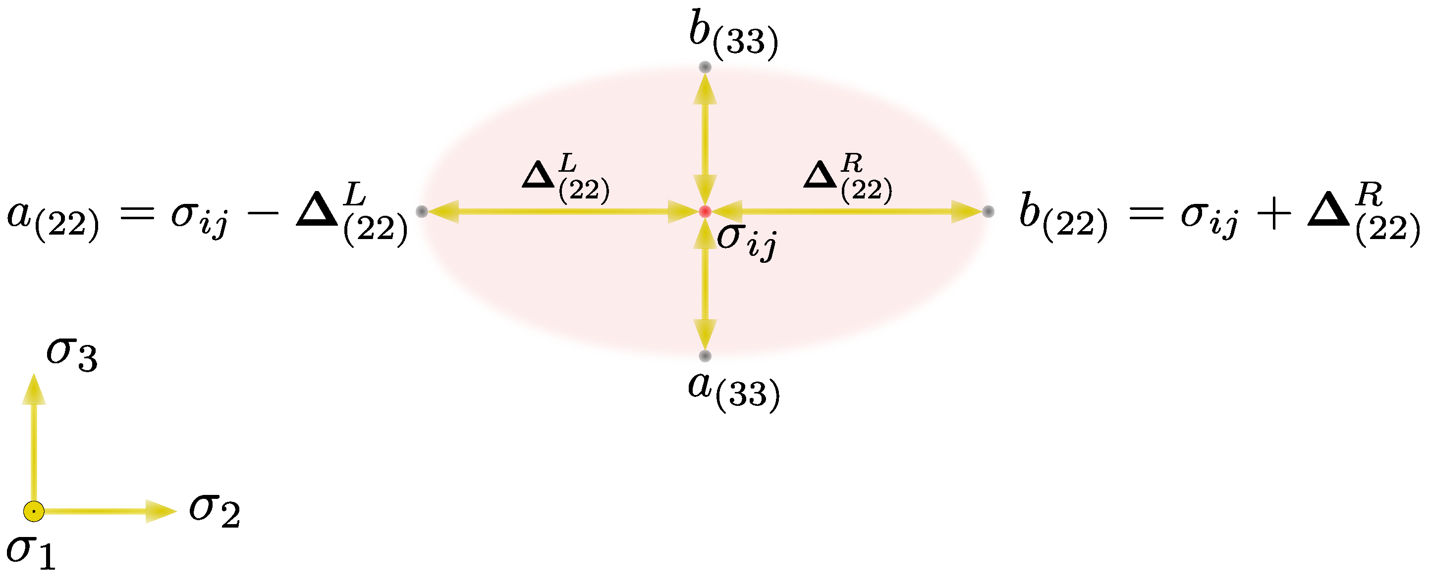
The interpretation of the virtual surrounding in a stress state depends on the specific material (see [28]), but in general it could be understood as a (homogenized) phenomenological measure of some instability, e.g., for metallic materials it is connected with dislocation nucleation [32,33,34], nucleation of voids [35] or breakup of grains [36,37,38] (see review paper [39]). By way of illustration, Figure 1 shows the cross-section of this virtual neighbourhood in the ${\sigma }_2-{\sigma }_3$ plane.

The analysis of Equation (21) shows differences in relation to the classical viscoplasticity where the change in volume may only occur in the elastic range—in the classical case, the trace of the $\mathbf{p}$ tensor equals 0. This condition is abandoned in the fractional formulation (when $\alpha \in (0,1)$), thus explicitly providing a tool to control the evolution of volume in the plastic range through $\alpha$ and parametric vectors ${\Delta }^{\mathbf{L}}$ and ${\Delta }^{\mathbf{R}}$. Moreover, the versatility of the fractional approach is proven for $\alpha =1$, for which the associated plastic flow as a special case is obtained.

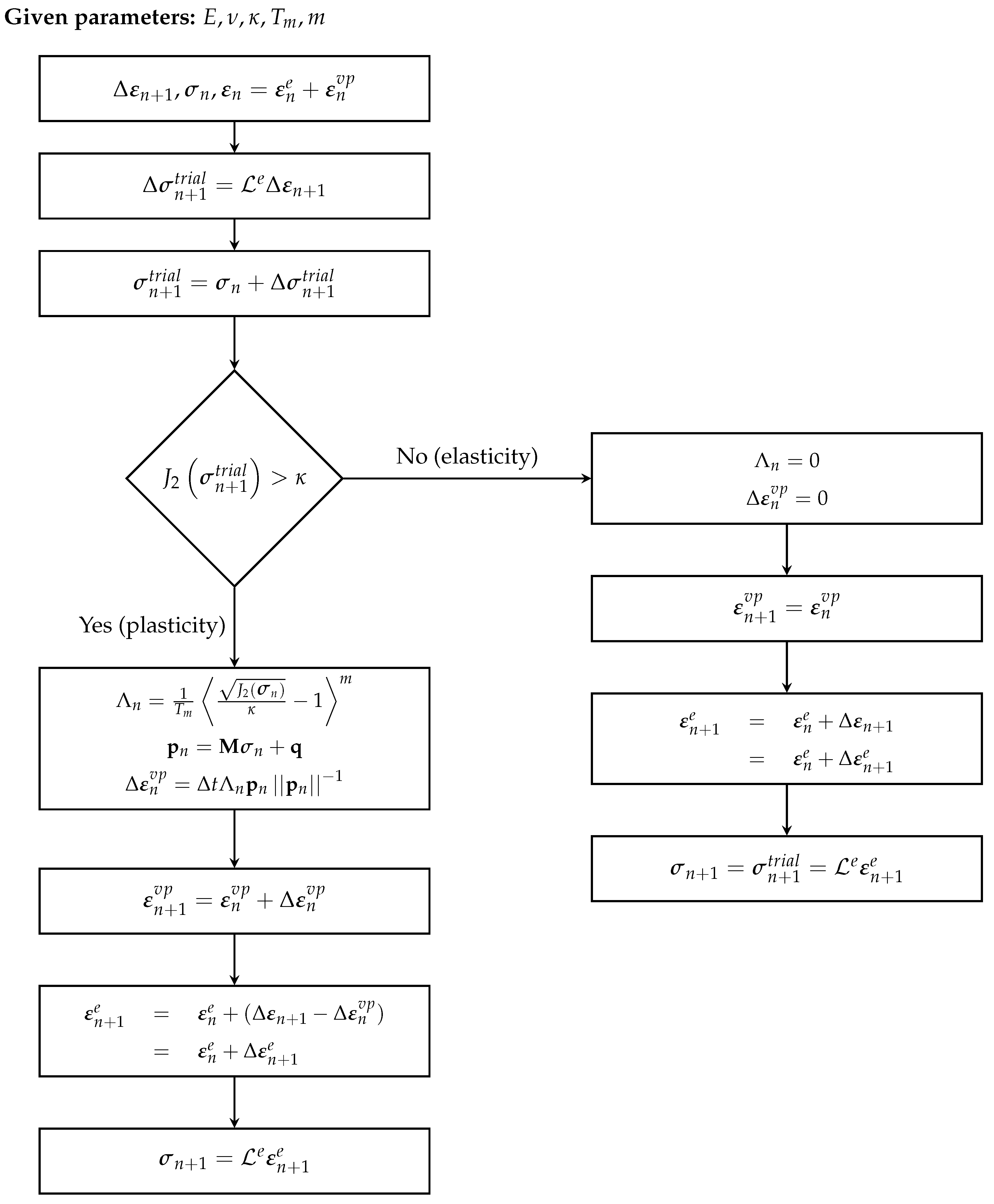
Finally, the flowchart was formulated that presents the general calculation scheme for the elasto-viscoplastic material in the framework of the fractional viscoplastic flow rule for explicit time integration in VUAMT subroutine (see Figure 2). The VUAMT subroutine aims at determination of the values of Cauchy stresses and updating strains and internal variables at time $t_{n+1}$ based on the knowledge of these parameters at the previous moment $t_n$. The procedure starts with the calculation of the elastic trial stress, which is later used to establish the value of the yield criterion. If this criterion is fulfilled, the plastic multiplier $\Lambda$ and the direction of plastic flow $\mathbf{p}$ are calculated according to the flow rule; otherwise the elastic step is conducted.

4. Parametric Study: Uniaxial Tension

4.1. Description of the Numerical Experiment

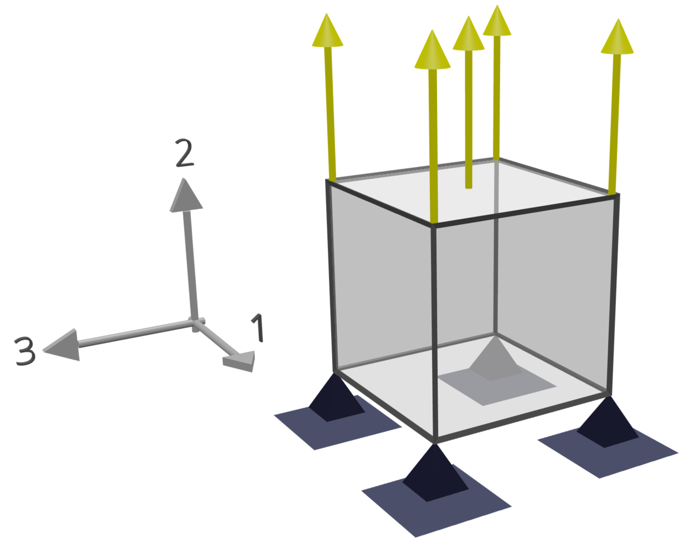
The conducted parametric study is focused on the material point level represented by a unit cube with dimensions of 1 × 1 × 1 mm discretized by a single finite element C38DR (linear, eight-node brick with reduce integration). The boundary conditions required to achieve uniaxial constraints are shown in Figure 3. Basic mechanical properties were assumed as for the carbon steel, therefore the elastic range was characterized by Young’s modulus E = 205 GPa and Poisson’s ratio $\nu$ = 0.27. The fractional flow rule presented in Section 2 was applied in the plastic range. The static yield stress in simple shear for the selected material was $\kappa$ = 605 MPa. Other material parameters, depending on the studied case, were chosen as described below.

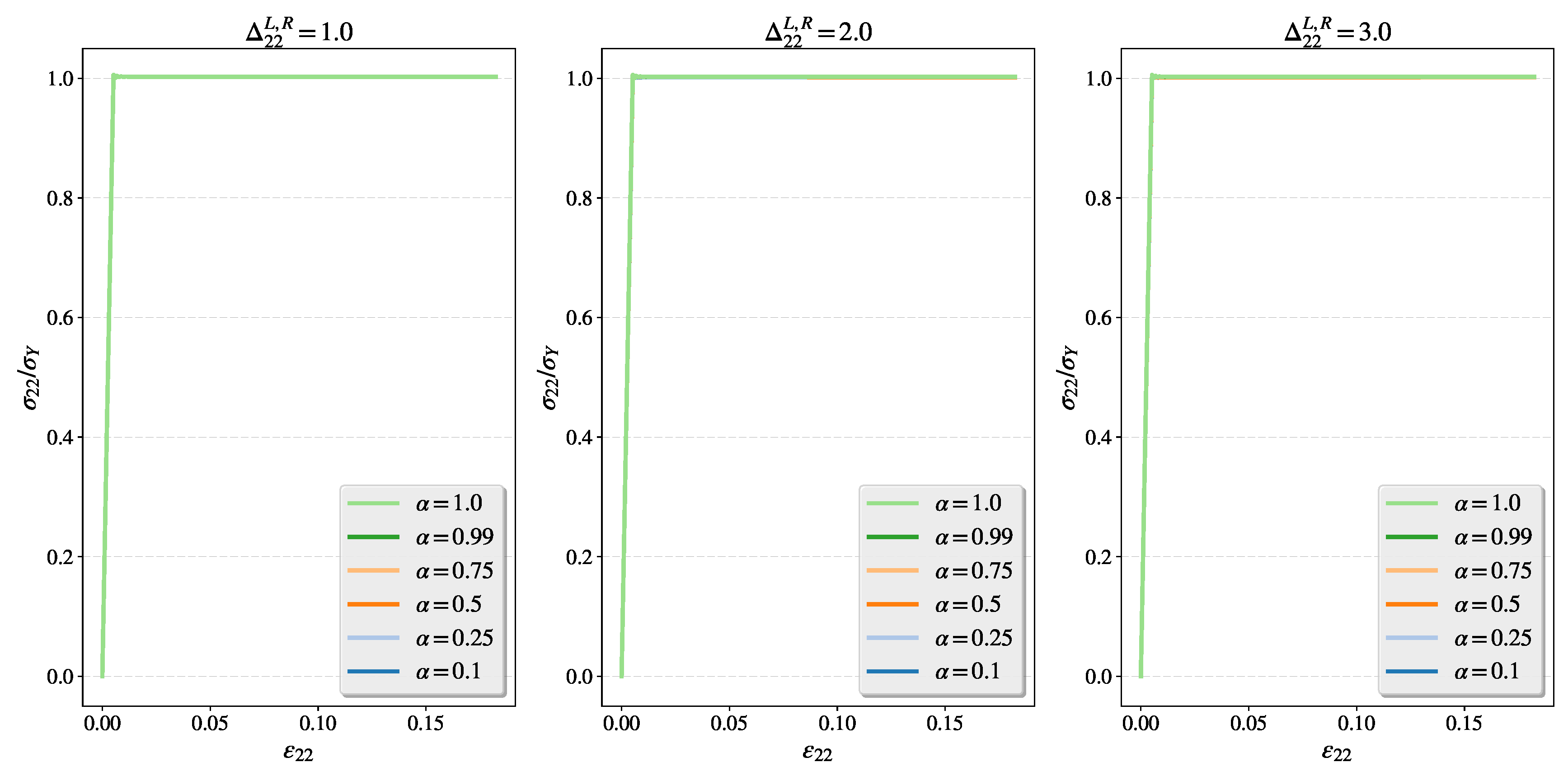
The analyzed cases of fractional flow were divided into two groups to show how various combinations of model parameters influence plastic deformation. The first group is focused on the value of the stress-fractional non-locality spread (${\Delta }^{L,R}$) and the order ($\alpha$) of the fractional flow. In the second group, the influence of the material parameters $T_m$ and m under various speeds of the imposed displacement is closely studied. Anticipating the anisotropic behaviour of the fractional material model, these two groups were further subdivided according to the direction where the dominant viscoplastic flow was expected. Hence, two cases were formed for tension direction (${\Delta }_{22}^{L,R}=0.005\kappa \approx 3.0\mathrm{MPa}$) and direction perpendicular to tension (${\Delta }_{11}^{L,R}=0.005\kappa \approx 3.0\mathrm{MPa}$). In each of those cases, other values of the $\Delta$ were set to $0.0017\kappa \approx 1.0\mathrm{MPa}$.

Two kinds of plots were used to present the results of the parametric study. The first kind exemplify the relation between three normal strains ${\epsilon }_{11},{\epsilon }_{22},{\epsilon }_{33}$. The second type shows the stress–strain relation in the tension (2) direction (it should be pointed out that for this kind of plots, a ‘softening’ is observed, especially for highest tension velocities, however, this effect is due to the lateral stresses induced by the inertia effects and is not due to constitutive model $\kappa =const.$ See Figure 4, where this effect is negligible due to relatively small tension velocity $v=1\frac{m}{s}$ ). The research on influence of the fractional derivative order was performed for a set $\alpha \in \{0.1,0.25,0.5,0.75,0.99,1.0\}$—as mentioned earlier, fractional generalization of the viscoplasticity reduces to the classical solution for $\alpha =1$. The study of $T_m$ and m was conducted for three different velocities of tension, i.e., $v=1$, 25 and $50\frac{m}{s}$.

4.2. Influence of the Order of FV and Non-Locality in a Stress State on Plastic Flow

4.2.1. Study of Intensified Plastic Flow in Tension Direction for Different Orders of Flow

Figure 4 presents the material response to the applied tension velocity of $v=1\frac{m}{s}$ for different flow intensities in tension direction and flow orders. Increasing the flow intensity parameter (${\Delta }^{L,R}$) causes higher evolution of the plastic flow in the chosen direction but in this case the velocity of the load is not sufficient to reveal different behaviour in the stress–strain relation for different values of $\alpha$ (see Figure 4). Next, for the same configuration of material parameters higher velocity is applied, namely $v=25\frac{m}{s}$. At this speed (Figure 5), a slight waveform begins to be visible for ${\Delta }_{22}^{L,R}=1.0\mathrm{MPa}$. The amplitude of the stress signal increases with the increases ${\Delta }_{22}^{L,R}$. Additionally, the influence of $\alpha$ is shown because the decrease in its value translates into greater amplitude of oscillations. So, we conclude that both fractional parameters, control the dynamic properties of a fractional model.

4.2.2. Study of Intensified Plastic Flow Perpendicular to the Tension Direction for Different Orders of Flow

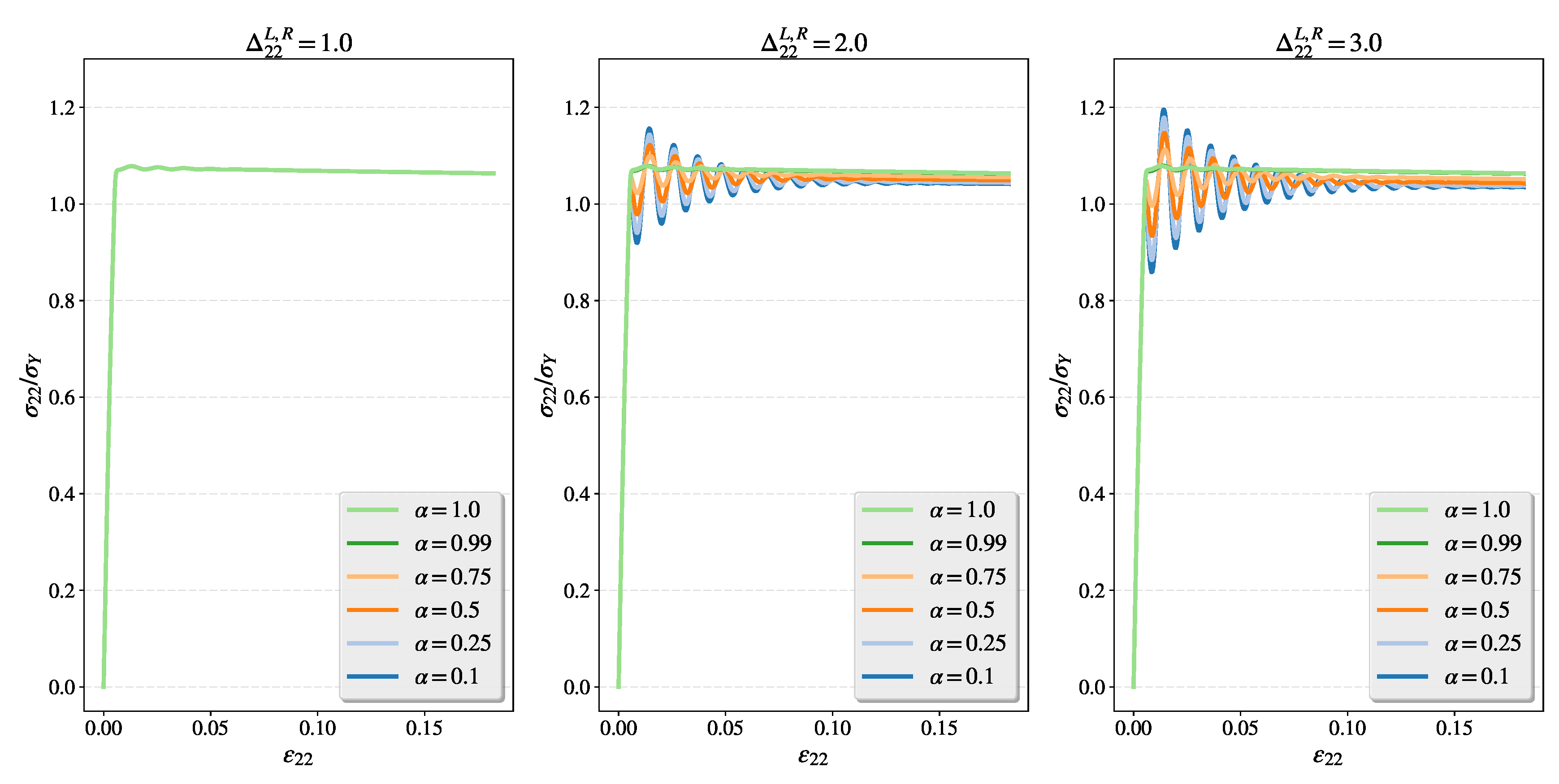
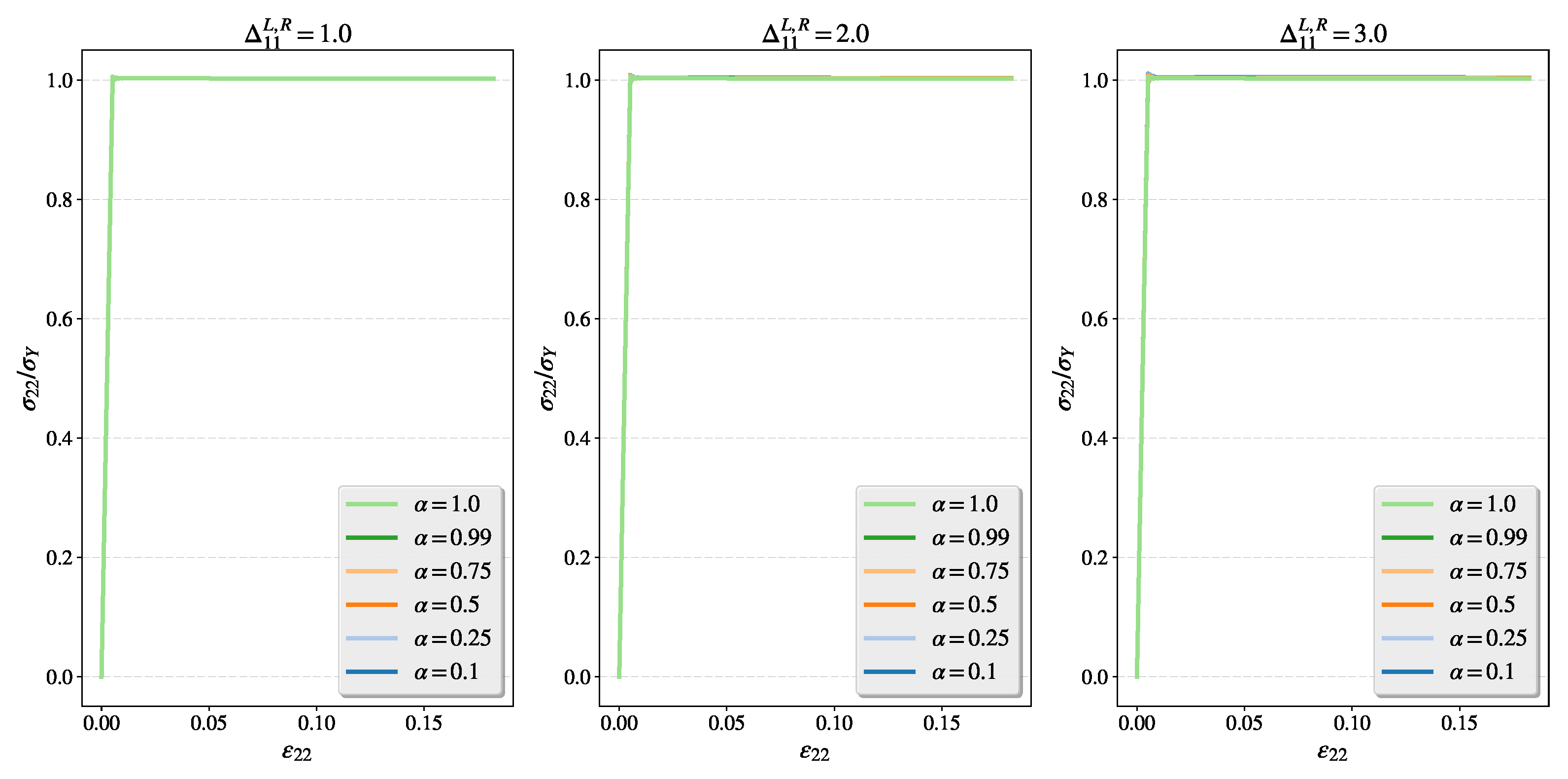
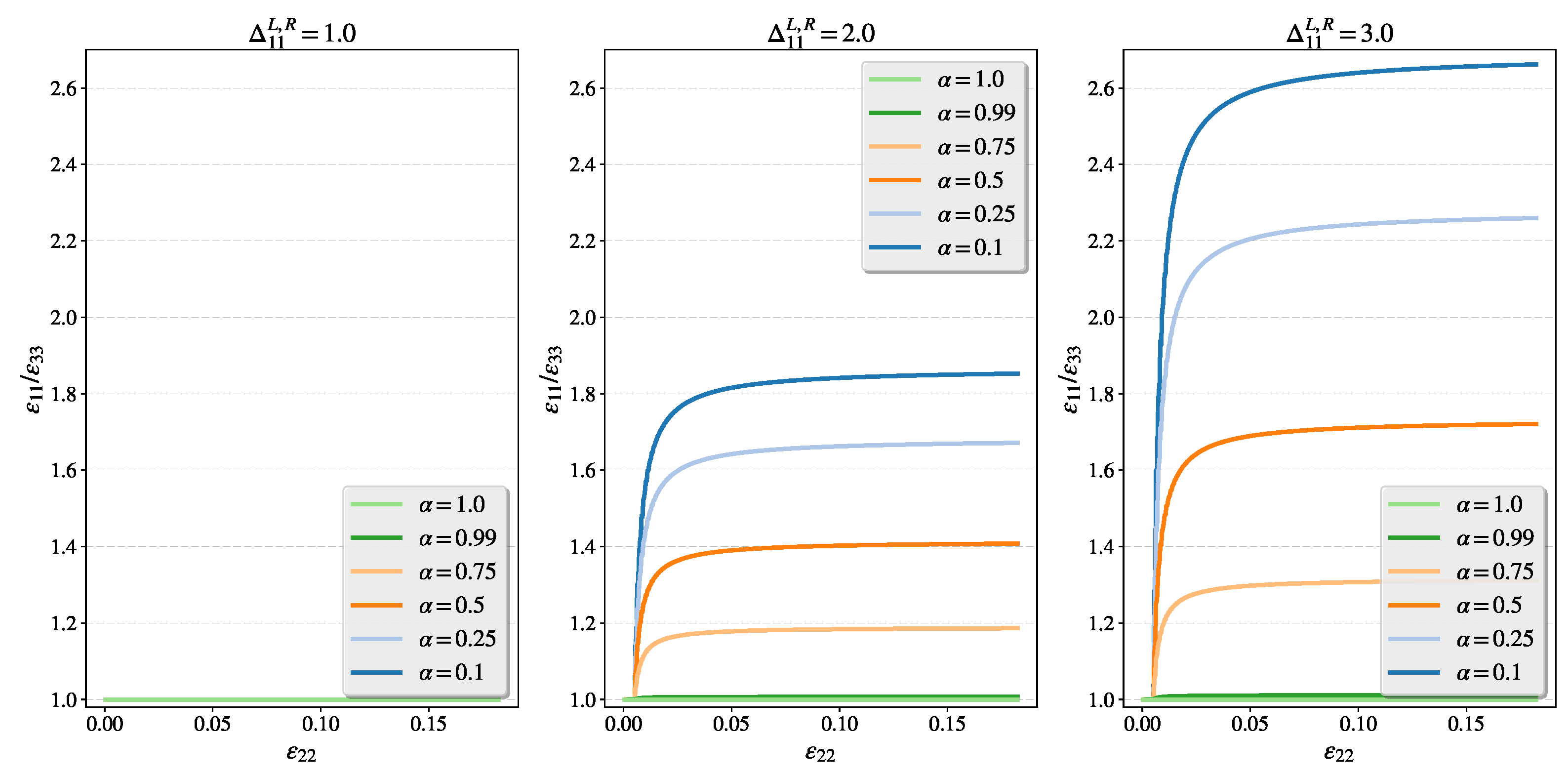
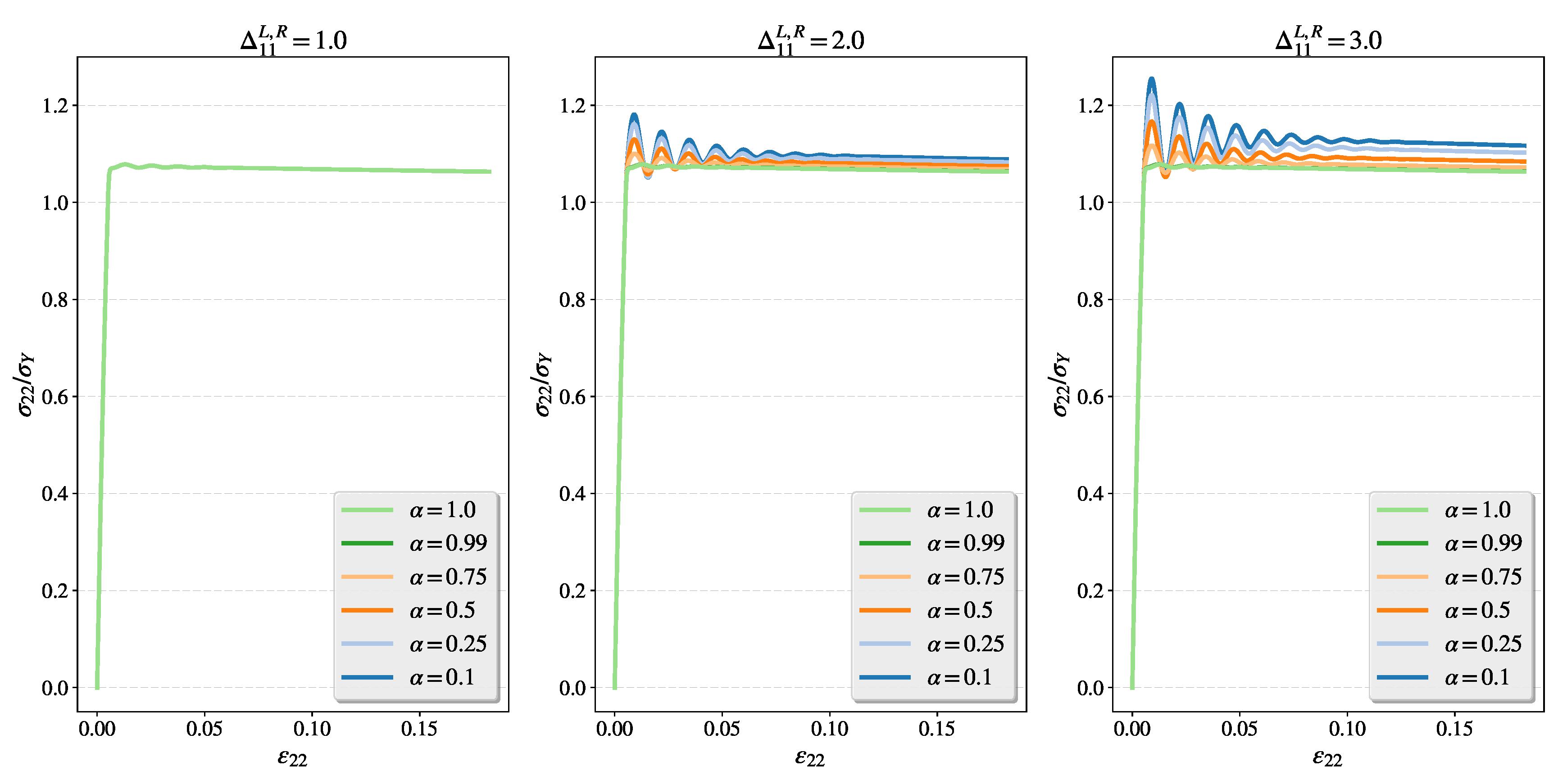
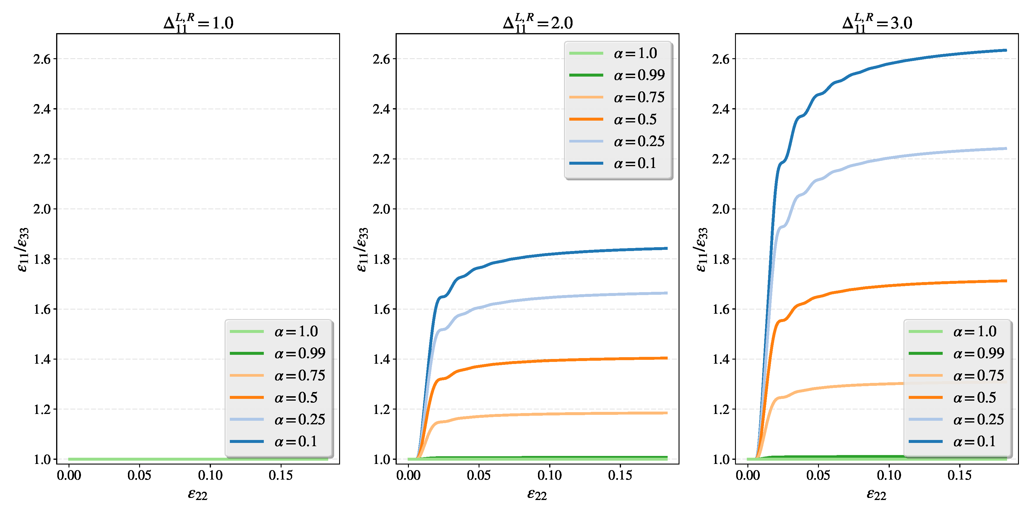
Results presented in this section were obtained for a parameter set similar to this in Section 4.2.1 with the difference that flow intensity is increased in the direction perpendicular to tension, namely ${\Delta }_{11}^{L,R}=3.0\mathrm{MPa}$. Others components of vectors in Equations (24) and (25) equal 1. As in the discussion in the previous section, the tension velocity of $v=1\frac{m}{s}$ is insufficient to reveal the influence of $\alpha$ on the stress–strain relation (see Figure 6). However, Figure 7 shows that the material prefers to deform in (1) direction when the magnitude of ${\Delta }_{11}^{L,R}$ growths, hence the ${\epsilon }_{11}/{\epsilon }_{33}$ ratio is greater then 1. Moreover, the intensity of the flow in the preferred direction increases as the value of $\alpha$ diminishes to 0. Next, as before, the velocity is increased to $v=25\frac{m}{s}$. Figure 8 shows that when the value of ${\Delta }^{L,R}$ rises, greater amplitude of the oscillation and hardening of the material can be observed. This last effect is inversely proportional to the order of the fractional flow. The relation between ${\epsilon }_{11},{\epsilon }_{22}$ and ${\epsilon }_{33}$ is presented in Figure 9 and is very similar to Figure 7 with the only distinction that slight oscillation occurs as a result of higher velocity. So, we conclude that both fractional parameters control the anisotropic properties of a fractional model in the plastic range.

4.3. Influence of the Relaxation Time and the Overstress Power

4.3.1. Study of the Fractional Flow Under Different Dynamic Loading Rates for Intensified Plastic Flow in Tension Direction

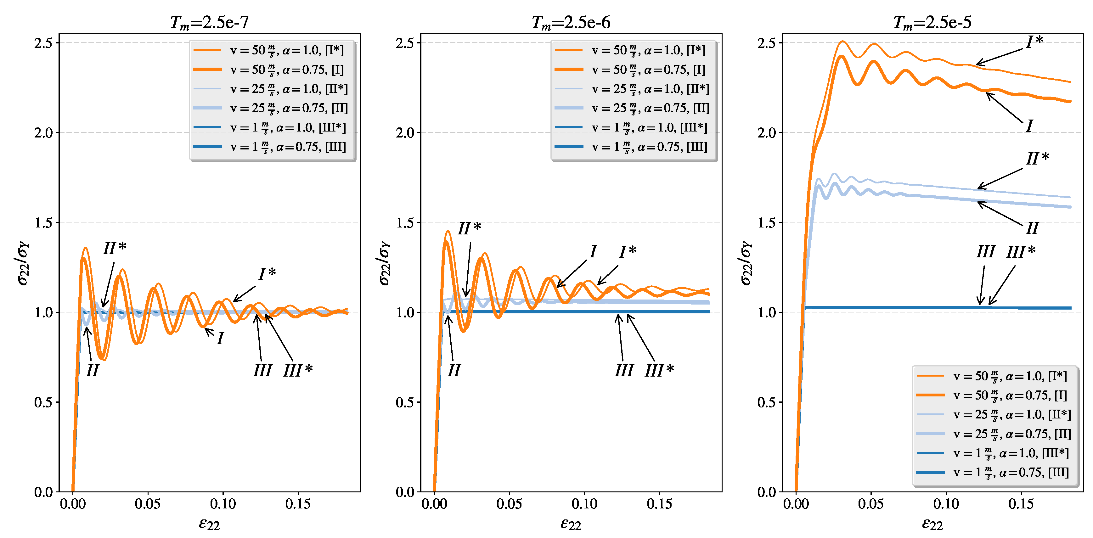
Here we assume that the intensified plastic flow, determined by ${\Delta }_{22}^{L,R}=3.0\mathrm{MPa}$, is in tension direction. Figure 10 presents the effect of different relaxation times for various velocities of tension. It should be pointed out that in order to increase clarity of interpretation both the classical ($\alpha =1$) and the fractional ($\alpha =0.75$) solutions are compared on each graph. As can be seen, when the relaxation time grows, the hardening of the material as well as the stress waves oscillations increase. The latter is especially pronounced for the relaxation time $T_m=2.5e-5s$.

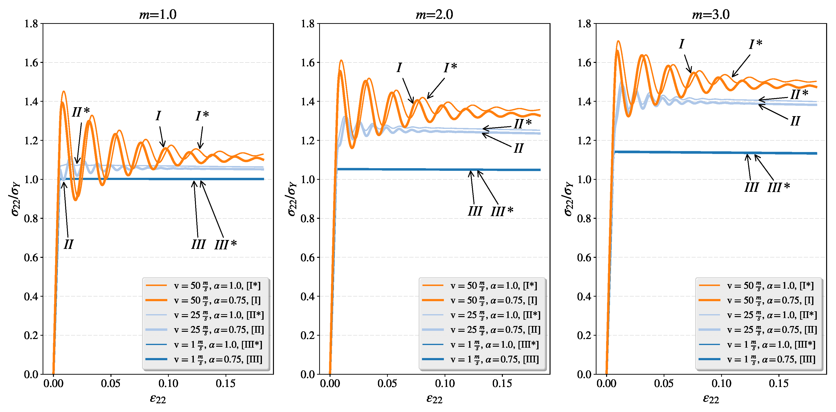
Figure 11 presents the result of increasing the value of the overstress parameter m. For the fractional ($\alpha =0.75$) viscoplastic material the stress level is smaller in relation to the classical ($\alpha =1.0$) viscoplastic solution (Figure 10 and Figure 11).

Results discussed above indicate that the relaxation time and overstress power, together with fractional parameters, control the level of strain rate hardening and stress waves oscillation amplitude.

4.3.2. Study of the Fractional Flow Under Different Dynamic Loading for the Intensified Plastic Flow Perpendicular to the Tension Direction

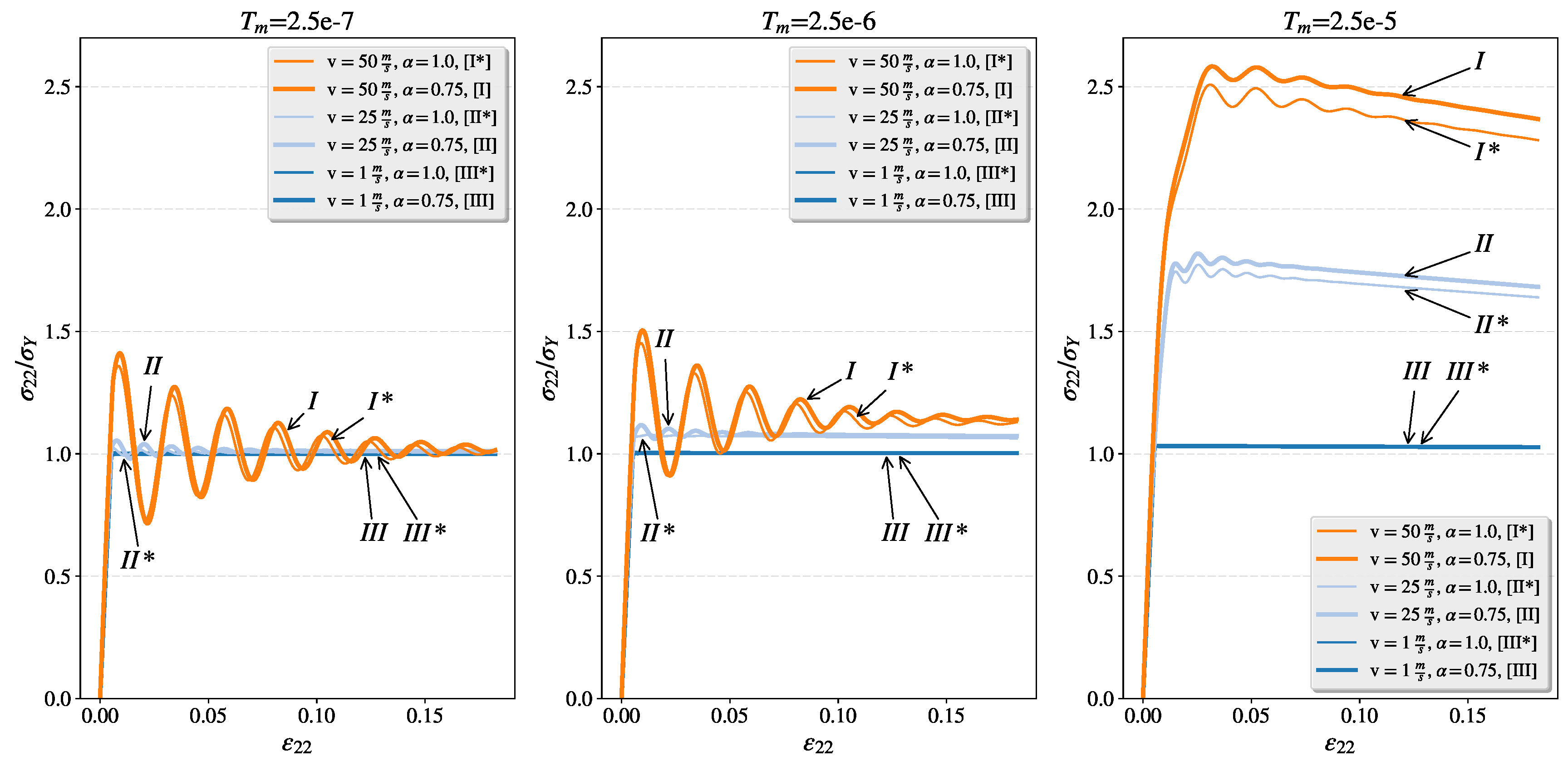
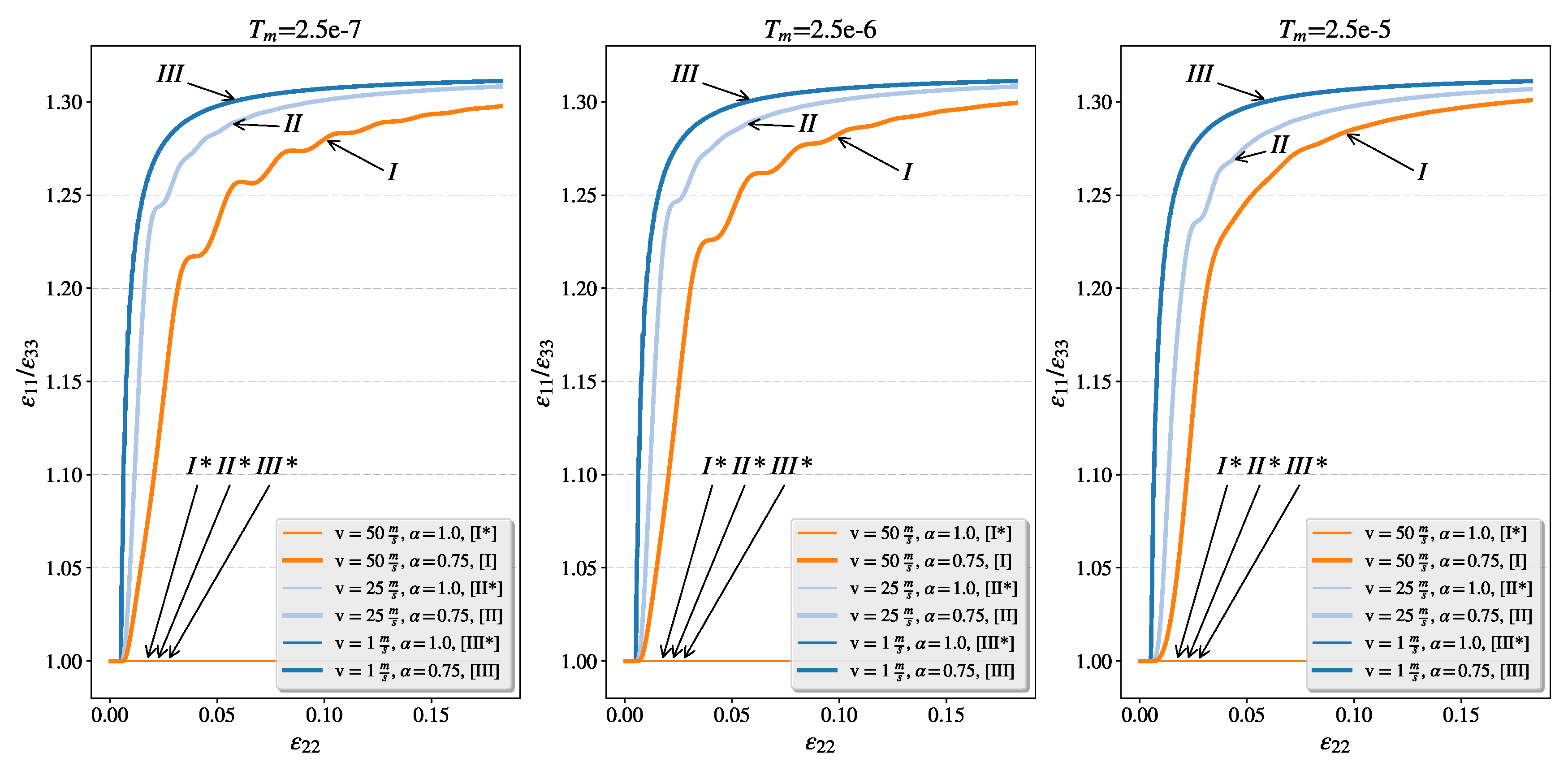
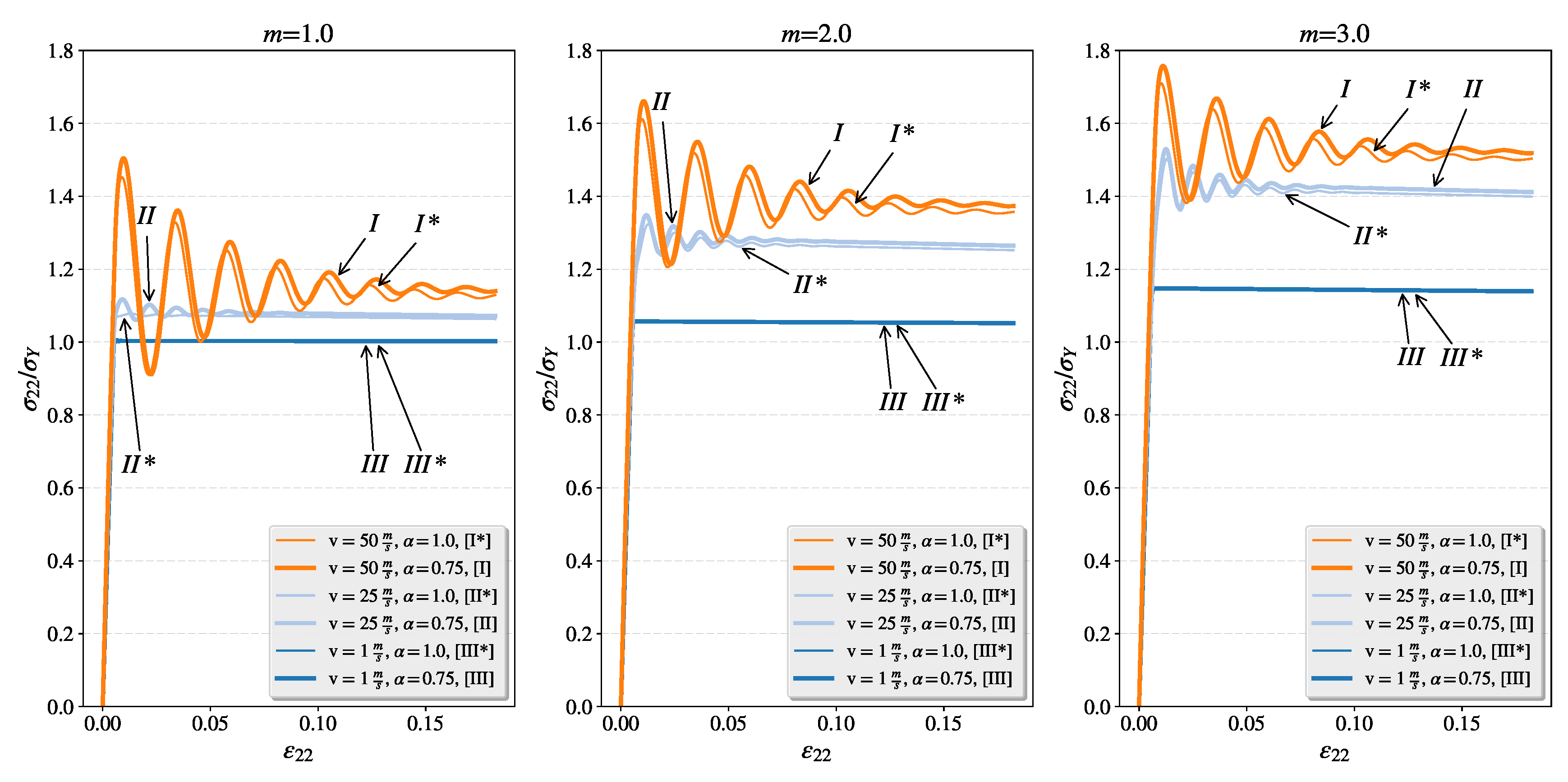
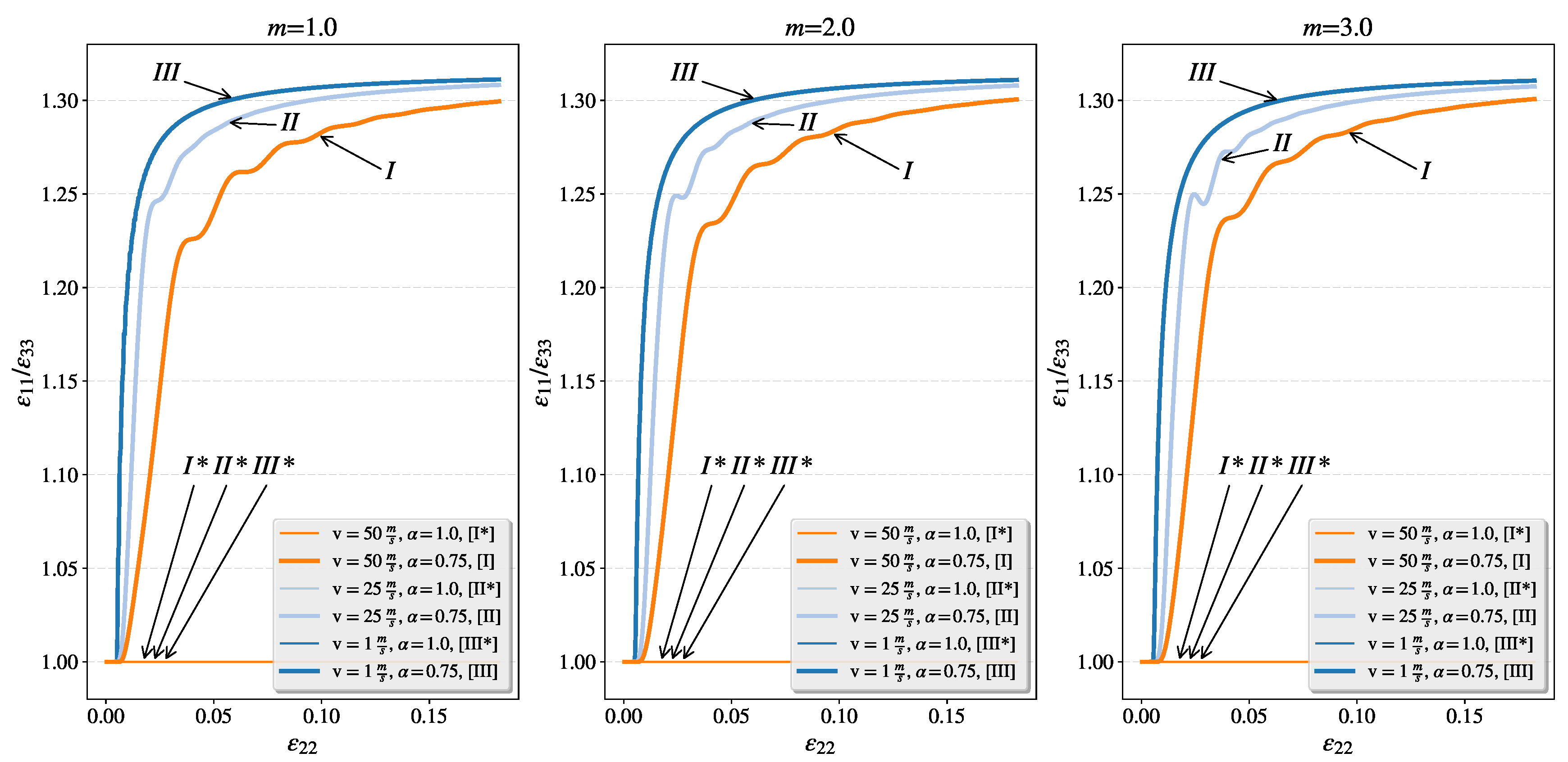
In this section, it is assumed that fractional flow is intensified in the direction perpendicular to tension load (${\Delta }_{11}^{L,R}=3.0MPa$). Figure 12 shows that raising relaxation time causes similar effects to those discussed in the previous section. The biggest change occurs for the relaxation time $T_m=2.5e-5s$ both in the stress level and the stress wave oscillations frequency. In Figure 13 a clear anisotropy of the plastic deformation for $\alpha =0.75$ can be noticed. As before, it is observed that increasing the value of m causes a growth in the material strain hardening without any apparent influence on the frequency of the stress wave (see Figure 14). By analogy to what is presented for $T_m$, in Figure 15 the dominant nature of ${\epsilon }_{11}$ can be observed, in addition to more pronounced oscillations for greater values of m. The analysis of the $\sigma -\epsilon$ relation for $\alpha =1$ and $\alpha =0.75$ also revealed that the stress levels of the fractional model are generally greater than for the classical solution (see Figure 12 and Figure 14). This last observation is different from what was discovered in the previous section.

In conclusion, as before, a prominent influence of the relaxation time and overstress power, together with fractional parameters, on the level of strain rate hardening and stress waves oscillation amplitude is observed. Additionally, the impact on dynamic properties of deformation anisotropy for fractional material was confirmed.

4.4. Study of the Disperse Character of the Fractional Viscoplastic Stress Waves

The last study performed was the analysis of the disperse character of the fractional viscoplastic stress waves. As shown in the previous sections, the uniaxial dynamic deformation induces a stress waves. The regularity of the oscillations was determined by averaging intervals between peaks and then calculating the frequency.

Table 1. The stress wave frequencies for $T_m=2.5e-6s$, $m=1$

		${\mathbf{\Delta }}_{22}=3.0$	${\mathbf{\Delta }}_{11}=3.0$
$v=25\frac{m}{s}$	$\alpha =1$	2.085 MHz	2.085 MHz
	$\alpha =0.75$	2.108 MHz	1.996 MHz
$v=50\frac{m}{s}$	$\alpha =1$	2.073 MHz	2.073 MHz
	$\alpha =0.75$	2.157 MHz	2.028 MHz

lists the stress wave frequencies for ${\Delta }_{22}^{L,R}=3.0\mathrm{MPa}$ and ${\Delta }_{11}^{L,R}=3.0\mathrm{MPa}$, which were depicted in the middle graphs of Figure 10 and Figure 12. The material parameter ${\Delta }^{L,R}$ does not appear in the classical viscoplasticity, so there is no change in the stress wave frequency for various values of this parameter when $\alpha =1$, thus tension velocity is only important. However, for fractional material, i.e., when $\alpha =0.75$, both flow intensity parameters and tension velocities modulate the frequency of stress waves. For $\alpha =0.75$ the frequencies are higher when the distinguished direction is co-linear with tension (${\Delta }_{22}=3.0\mathrm{MPa}$).

The results presented in

Table 2. The stress wave frequencies for ${\Delta }_{22}=3.0MPa$, $v=50\frac{m}{s}$

		${\mathit{T}}_{\mathit{m}}$
		2.5e-7	2.5e-6	2.5e-5
$m=1$	$\alpha =1$	2.073 MHz	2.073MHz	2.274 MHz
	$\alpha =0.75$	2.157 MHz	2.157 MHz	2.288 MHz
$m=2$	$\alpha =1$	2.073 MHz	2.085 MHz	2.182 MHz
	$\alpha =0.75$	2.157 MHz	2.157 MHz	2.207 MHz
$m=3$	$\alpha =1$	2.073 MHz	2.085 MHz	2.169 MHz
	$\alpha =0.75$	2.157 MHz	2.157 MHz	2.182 MHz

correspond to the investigation of the role of the relaxation time and overstress power discussed in Section 4.3. Regardless of the value of $\alpha$, the largest change in frequency can be observed between columns 2 and 3, that is for $T_m=2.5e-6s$ and $T_m=2.5e-5s$. The comparison of the values in columns 1 ($T_m=2.5e-7s$) and 2 ($T_m=2.5e-6s$) shows that the stress wave frequencies are the same or very similar. The impact of m shows that the significant influence of this parameter was only recorded for $T_m=2.5e-5s$. For both $\alpha =0.75$ and $\alpha =1$ the increase of the overstress power results in the increase of the frequency of the stress wave.

One concludes that the relaxation time and overstress power, together with fractional parameters, control the dispersive character of stress waves, and even more, makes this attribute directional.

5. Conclusions

The analysis of the dynamic properties of the Perzyna model of viscoplasticity (implicit time, non-local) generalized using fractional calculus (explicit, stress-fractional, non-local) leads to the following conclusions:

• Fractional viscoplasticity introduces an additional set of material parameters, namely flow order $\alpha$ and virtual stress state surrounding $\Delta$.
• Fractional parameters $\alpha$ and $\Delta$ control the dynamic properties of the fractional model, especially hardening, the character of the stress waves, and plastic anisotropy.
• The direction of the flow vector is controlled by $\Delta$, which in general leads to non-normality of plastic flow.
• As in the classical Perzyna model, the relaxation time $T_m$ and the overstress power m affect the strain rate hardening and the character of the stress waves.
• Induced plastic anisotropy of the fractional model should be regarded not only in the classical sense as directional deformation but also as directional viscosity, which results in directional dispersive character.

The above results are fundamental from the point of view of modeling strain localization and damage phenomena. Both these aspects will serve as a base for future studies.

References

- Podlubny, I. Fractional Differential Equations. In Mathematics in Science and Engineering; Academin Press: Cambridge, MA, USA, 1999; Volume 198. [Google Scholar]
- Samko, S.; Kilbas, A.; Marichev, O. Fractional Integrals and Derivatives: Theory and Applications; Gordon and Breach: Amsterdam, The Netherlands, 1993. [Google Scholar]
- Meng, R.; Yin, D.; Zhou, C.; Wu, H. Fractional description of time-dependent mechanical property evolution in materials with strain softening behavior. Appl. Math. Modell. 2016, 40, 398–406. [Google Scholar] [CrossRef]
- Li, M. Three Classes of Fractional Oscillators. Symmetry 2018, 10, 40. [Google Scholar] [CrossRef]
- Zhao, J.; Zheng, L.; Zhang, X.; Liu, F. Convection heat and mass transfer of fractional MHD Maxwell fluid in a porous medium with Soret and Dufour effects. Int. J. Heat Mass Trans. 2016, 103, 203–210. [Google Scholar] [CrossRef]
- Jinhu, Z.; Liancun, Z.; Xinxin, Z.; Fawang, L. Mixed convection heat transfer of viscoelastic fluid along an inclined plate obeying the fractional constitutive laws. Heat Trans. Res. 2017, 48, 1165–1178. [Google Scholar]
- Zhang, X.; Liu, L.; Wu, Y. The uniqueness of positive solution for a fractional order model of turbulent flow in a porous medium. Appl. Math. Lett. 2014, 37, 26–33. [Google Scholar] [CrossRef]
- Cherniha, R.; Gozak, K.; Waniewski, J. Exact and Numerical Solutions of a Spatially-Distributed Mathematical Model for Fluid and Solute Transport in Peritoneal Dialysis. Symmetry 2016, 8, 50. [Google Scholar] [CrossRef]
- Atanackovic, T.; Janev, M.; Oparnica, L.; Pilipovic, S.; Zorica, D. Space–time fractional Zener wave equation. Proc. Math. Phys. Eng. Sci. 2015, 471, 20140614. [Google Scholar]
- Ren, T.; Li, S.; Zhang, X.; Liu, L. Maximum and minimum solutions for a nonlocal p-Laplacian fractional differential system from eco-economical processes. Bound. Value Probl. 2017, 2017, 118. [Google Scholar] [CrossRef]
- Sumelka, W.; Voyiadjis, G. A hyperelastic fractional damage material model with memory. Int. J. Solids Struct. 2017, 124, 151–160. [Google Scholar] [CrossRef]
- Klimek, M. Fractional sequential mechanics—Models with symmetric fractional derivative. Czechoslov. J. Phys. 2001, 51, 1348–1354. [Google Scholar] [CrossRef]
- Drapaca, C.; Sivaloganathan, S. A Fractional Model of Continuum Mechanics. J. Elast. 2012, 107, 107–123. [Google Scholar] [CrossRef]
- Sumelka, W.; Szajek, K.; Łodygowski, T. Plane strain and plane stress elasticity under fractional continuum mechanics. Arch. Appl. Mech. 2015, 89, 1527–1544. [Google Scholar] [CrossRef]
- Tomasz, B. Analytical and numerical solution of the fractional Euler–Bernoulli beam equation. J. Mech. Mater. Struct. 2017, 12, 23–34. [Google Scholar]
- Lazopoulos, K.; Lazopoulos, A. Fractional vector calculus and fluid mechanics. J. Mech. Behav. Mater. 2017, 26, 43–54. [Google Scholar] [CrossRef]
- Peter, B. Dynamical Systems Approach of Internal Length in Fractional Calculus. Eng. Trans. 2017, 65, 209–215. [Google Scholar]
- Sumelka, W. Fractional viscoplasticity. Mech. Res. Commun. 2014, 56, 31–36. [Google Scholar] [CrossRef]
- Sun, Y.; Shen, Y. Constitutive model of granular soils using fractional-order plastic-flow rule. Int. J. Geomech. 2017, 17, 04017025. [Google Scholar] [CrossRef]
- Sun, Y.; Xiao, Y. Fractional order model for granular soils under drained cyclic loading. Int. J. Numer. Anal. Meth. Geomech. 2017, 41, 555–577. [Google Scholar] [CrossRef]
- Sun, Y.; Xiao, Y. Fractional order plasticity model for granular soils subjected to monotonic triaxial compression. Int. J. Solids Struct. 2017, 118-119, 224–234. [Google Scholar] [CrossRef]
- Perzyna, P. The constitutive equations for rate sensitive plastic materials. Q. Appl. Math. 1963, 20, 321–332. [Google Scholar] [CrossRef] [Green Version]
- Glema, A.; Łodygowski, T. On importance of imperfections in plastic strain localization problems in materials under impact loading. Arch. Mech. 2002, 54, 411–423. [Google Scholar]
- Glema, A. Analysis of wave nature in plastic strain localization in solids. In Rozprawy; Publishing House of Poznan University of Technology: Poznan, Poland, 2004; Volume 379. (In Polish) [Google Scholar]
- Glema, A.; Łodygowski, T.; Perzyna, P. Interaction of deformation waves and localization phenomena in inelastic solids. Comput. Meth. Appl. Mech. Eng. 2000, 183, 123–140. [Google Scholar] [CrossRef] [Green Version]
- Glema, A.; Łodygowski, T.; Perzyna, P. Localization of plastic deformations as a result of wave interaction. Comput. Assist. Mech. Eng. Sci. 2003, 10, 81–91. [Google Scholar]
- Perzyna, P. The Thermodynamical Theory of Elasto-Viscoplasticity. Eng. Trans. 2005, 53, 235–316. [Google Scholar]
- Sumelka, W.; Nowak, M. Non-normality and induced plastic anisotropy under fractional plastic flow rule: A numerical study. Int. J. Numer. Anal. Meth. Geomech. 2016, 40, 651–675. [Google Scholar] [CrossRef]
- Sumelka, W.; Nowak, M. On a general numerical scheme for the fractional plastic flow rule. Mech. Mater. 2017, 116, 120–129. [Google Scholar] [CrossRef]
- Xiao, R.; Sun, H.; Chen, W. A finite deformation fractional viscoplastic model for the glass transition behavior of amorphous polymers. Int. J. Non-Linear Mech. 2017, 93, 7–14. [Google Scholar] [CrossRef]
- Odzijewicz, T.; Malinowska, A.; Torres, D. Green’s theorem for generalized fractional derivatives. Fract. Calc. Appl. Anal. 2013, 16, 64–75. [Google Scholar] [CrossRef] [Green Version]
- Ziegler, H. An Introduction to Thermomechanics; North Holland Series in Applied Mathematics and Mechanics; North-Holland Publishing Company: North Holland, The Netherlands, 1983; Volume 21. [Google Scholar]
- Dao, M.; Asaro, R. Non-Schmid effects and localized plastic flow in intermetallic alloys. Mater. Sci. Eng. A 1993, 170, 143–160. [Google Scholar] [CrossRef]
- Racherla, V.; Bassani, J. Strain burst phenomena in the necking of a sheet that deforms by non-associated plastic flow. Modell. Simul. Mater. Sci. Eng. 2007, 15, S297–S311. [Google Scholar] [CrossRef]
- Marin, E.; McDowell, D. Models for Compressible Elasto-Plasticity Based on Internal State Variables. Int. J. Damage Mech. 1998, 7, 47–83. [Google Scholar] [CrossRef] [Green Version]
- Leffers, T. Lattice rotations during plastic deformation with grain subdivision. Mater. Sci. Forum 1994, 157–162, 1815–1820. [Google Scholar] [CrossRef]
- Hughes, D.; Liu, Q.; Chrzan, D.; Hansen, N. Scaling of microstructural parameters: Misorientations of deformation induced boundaries. Acta Mater. 1997, 45, 105–112. [Google Scholar] [CrossRef]
- Steinmann, P.; Kuhl, E.; Stein, E. Aspects of non-associated single crystal plasticity: Influence of non-schmid effects and localization analysis. Int. J. Solids Struct. 1998, 35, 4437–4456. [Google Scholar] [CrossRef]
- McDowell, D. Viscoplasticity of heterogeneous metallic materials. Mater. Sci. Eng. R 2008, 62, 67–123. [Google Scholar] [CrossRef]
Figure 1.
Virtual surrounding of a material point.
Figure 2.
VUMAT subroutine flowchart for the fractional viscoplastic rule.
Figure 3.
Unit cubic model restricted to uniaxial tension.
Figure 4.
Influence of the order and the value of material parameter on the stress–strain relation, for: .
Figure 5.
Figure 6.
Figure 7.
Influence of the order and the value of material parameter on the relation between three normal stresses, for: .
Figure 8.
Figure 9.
Figure 10.
Influence of the relaxation parameter and the value of applied velocity field v on the stress–strain relation, for: .
Figure 11.
Influence of the material parameter m and the value of applied velocity field v on the stress–strain relation, for: .
Figure 12.
Figure 13.
Influence of the relaxation parameter and the value of applied velocity field v on the relation between three normal stresses, for: .
Figure 14.
Figure 15.
Influence of the material parameter m and the value of applied velocity field v on the relation between three normal stresses, for: .