Computing Metric Dimension and Metric Basis of 2D Lattice of Alpha-Boron Nanotubes

Abstract

Concepts of resolving set and metric basis has enjoyed a lot of success because of multi-purpose applications both in computer and mathematical sciences. For a connected graph G(V,E) a subset W of V(G) is a resolving set for G if every two vertices of G have distinct representations with respect to W. A resolving set of minimum cardinality is called a metric basis for graph G and this minimum cardinality is known as metric dimension of G. Boron nanotubes with different lattice structures, radii and chirality’s have attracted attention due to their transport properties, electronic structure and structural stability. In the present article, we compute the metric dimension and metric basis of 2D lattices of alpha-boron nanotubes.

1. Introduction

In a complex network, one is always interested to uniquely identify the location of nodes by assigning an address with reference to a particular set. Such a particular set with minimum possible nodes is known as the metric basis and its cardinality is known as the metric dimension.

These facts have been efficiently utilized in drug design to attack on particular nodes. Some computational aspects of carbon and boron nanotubes have been summed up in [1]. Similarly, a moving point in a graph may be located by finding the distance from the point to the collection of sonar stations, which have been properly positioned in the graph [2]. Thus, finding a minimal sufficiently large set of labeled vertices, such that a robot can find its position, is a problem known as robot navigation, already well-studied in [3]. This sufficiently large set of labeled vertices is a resolving set of the graph space and the cardinality of such a set with minimum possible elements is the metric dimension. Similarly, on another node, a real-world problem is the study of networks whose structure has not been imposed by a central authority but is also brought into light from local and distributed processes. Obtaining a map of all nodes and the links between them is difficult as well as expensive. To have a good approximation of the real network, a frequently used technique is to attain a local view of network from multiple dimensions and join them. The metric dimension also has some applications in this respect as well.

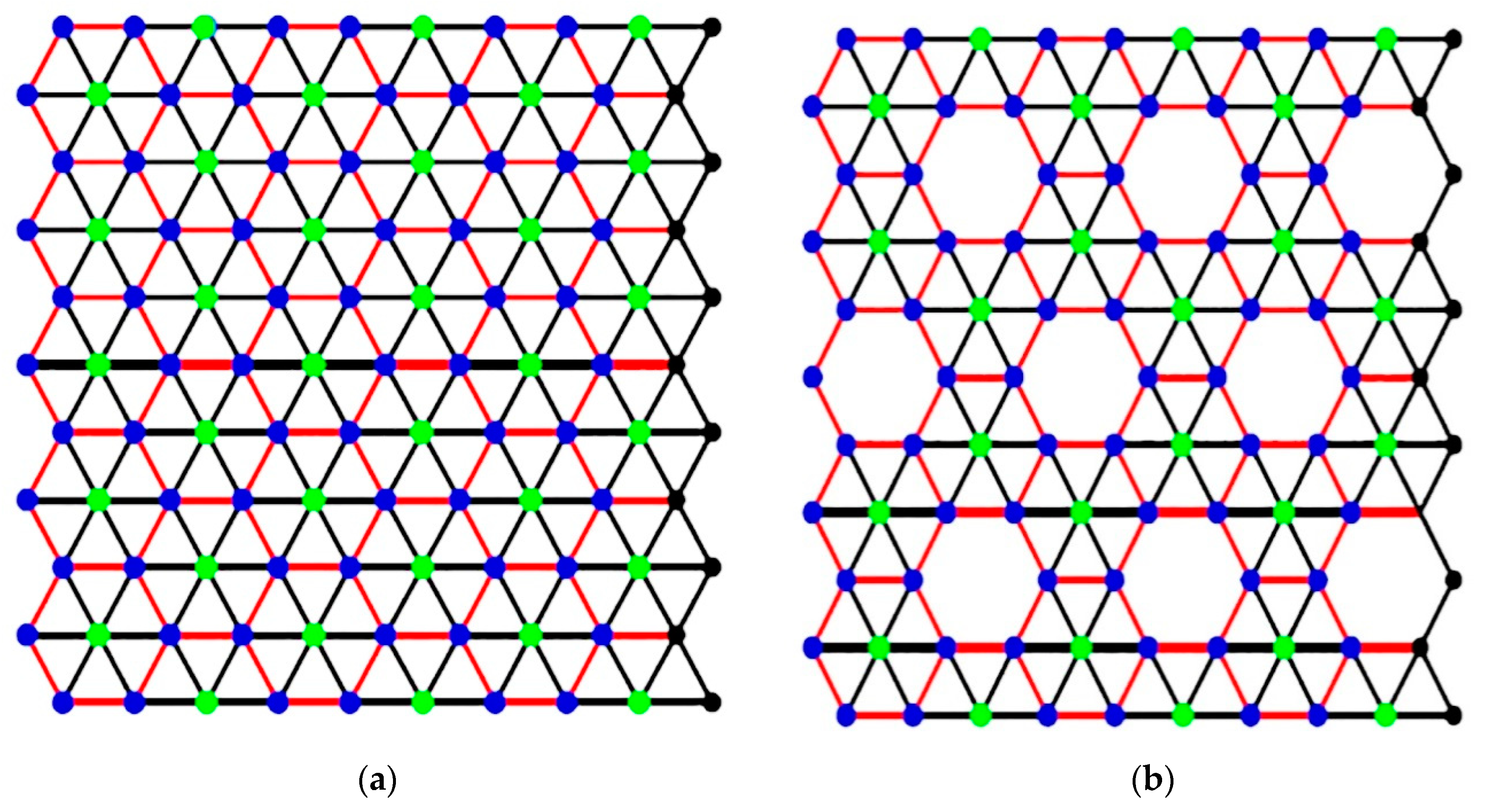
In nanomaterials, nanowires, nanocrystals, and nanotubes formulate three main classes. Boron nanotubes are becoming highly attractive due to their extraordinary features, including work function, transport properties, electronic structure, and structural stability, [3,4]. Triangular boron and α-boron are deduced from a triangular sheet and an α-sheet as shown in Figure 1 below.

The first boron nanotubes were made, in 2004, from a buckled triangular latticework [4]. The other famous type, alpha-boron, is constructed from an α-sheet. Both types are more conductive than carbon nanotubes regardless of their structure and chiralities. Due to an additional atom at the center of some of the hexagons, alpha-boron nanotubes have a more complex structure than triangular boron nanotubes [4]. This structure is the most stable known theoretical structure for boron nanotubes. With this specimen, boron nanotubes should have variable electrical properties, where wider ones should be metallic conductors, but narrower ones should be semiconductors. These tubes will replace carbon nanotubes in Nano devices like diodes and transistors. The following figure represents alpha-boron nanotubes.

The subject matter of the present article is the metric dimension of the 2D-lattices of alpha-boron nanotubes. An elementary problem in chemistry is to provide a distinct mathematical representation for the set of atoms, molecules, or compounds in a big structure. Consequently, the huge structure of a chemical compound under discussion can be represented by a labeled graph whose vertex and edge labels specify the atom and bond types, respectively. So, a graph-theoretic interpretation of this problem is to provide unique mathematical representations for the vertices of a graph in such a way that distinct vertices have distinct representations [5]. Going with a similar idea, we associate a 2D planar graph corresponding to the structure where nodes or vertices are represented for atoms, and where edges are actually the bonds between them. For the basics of graph theory, we refer to [6].

Let G be a connected graph and u, w be any two vertices of G. The length of the shortest path between u and w is called the distance between u and w and the number of edges between u and v in this shortest path is denoted by $d(u,v)$. Let $W=\left\{w_1,w_2,w_3,\dots ,w_n\right\}$ be an ordered set of vertices of G and v $\in$ V(G). The k-vector $\left(d\left(v,w_1\right),d\left(v,w_2\right),d\left(v,w_3\right),\dots ,d\left(v,w_n\right)\right)$ is called the representation $r(v|w)$ of $v$ with respect to $w$. If the distinct vertices of G have a distinct representation with respect to $w$, then $w$ is called a resolving set of G (see [7,8,9,10]). A resolving set of minimum cardinality is called a basis of G and this minimum cardinality is the metric dimension of G, denoted by dim(G).

The concept of the metric dimension was first crafted for metric spaces of a continuous nature but later on, these concepts were used for graphs. In fact, Slater initiated the concepts of metric dimension and resolving sets and these concepts were also studied by Melter and Harary independently in [11,12]. Resolving sets have been analyzed a lot since then. The resolving sets have applications in many fields including network discovery and verification [13], connected joins in graphs, strategies for the mastermind games [14], applications to problems of pattern recognition, image processing, combinatorial optimization, pharmaceutical chemistry, and game theory. In [8,10], authors computed metric dimension of some graphs and proved that it is 1 if and only if graph is the path $P_n$. The metric dimension of complete graph $K_n$ is $n-1$ for $n>1$ and the metric dimension of cycle graph $C_n$ is 2 for $n>1$ [8]. In [7], authors computed the metric dimension of the Cartesian products of some graphs. In [9], Imran et al. computed the metric dimension of the generalized Peterson graph. Also, generalized Petersen graphs $p(n,2)$, antiprisms $A_n$, and circulant graphs $C_n(1,2)$ are families of graphs with a constant metric dimension [15]. In [16], Imran et. al. discussed some families of graphs with a constant metric dimension. Ali et al. computed partial results about the metrics dimension of classical Mobius Ladders in [17], whereas Munir et al. computed the exact and full results for this family in [18]. In [19], authors computed the metric dimension of a generalized wheel graph and ant-web gear graph. Authors also gave a new family of convex polytopes with an unbounded metric dimension [19]. Recently authors in [20] computed metric dimension of some families of Gear graphs. Manuel et. al. computed the metric dimension of a honey-comb network in [21]. In [22], the authors computed the metric dimension of circulant graphs. In [23], authors computed explicit formula for the metric dimension of a regular bipartite graph. Imran et al. computed the metric dimension of a Jahangir graph in [24]. Authors discussed the metric dimension of the circulant and Harary graph in [25].

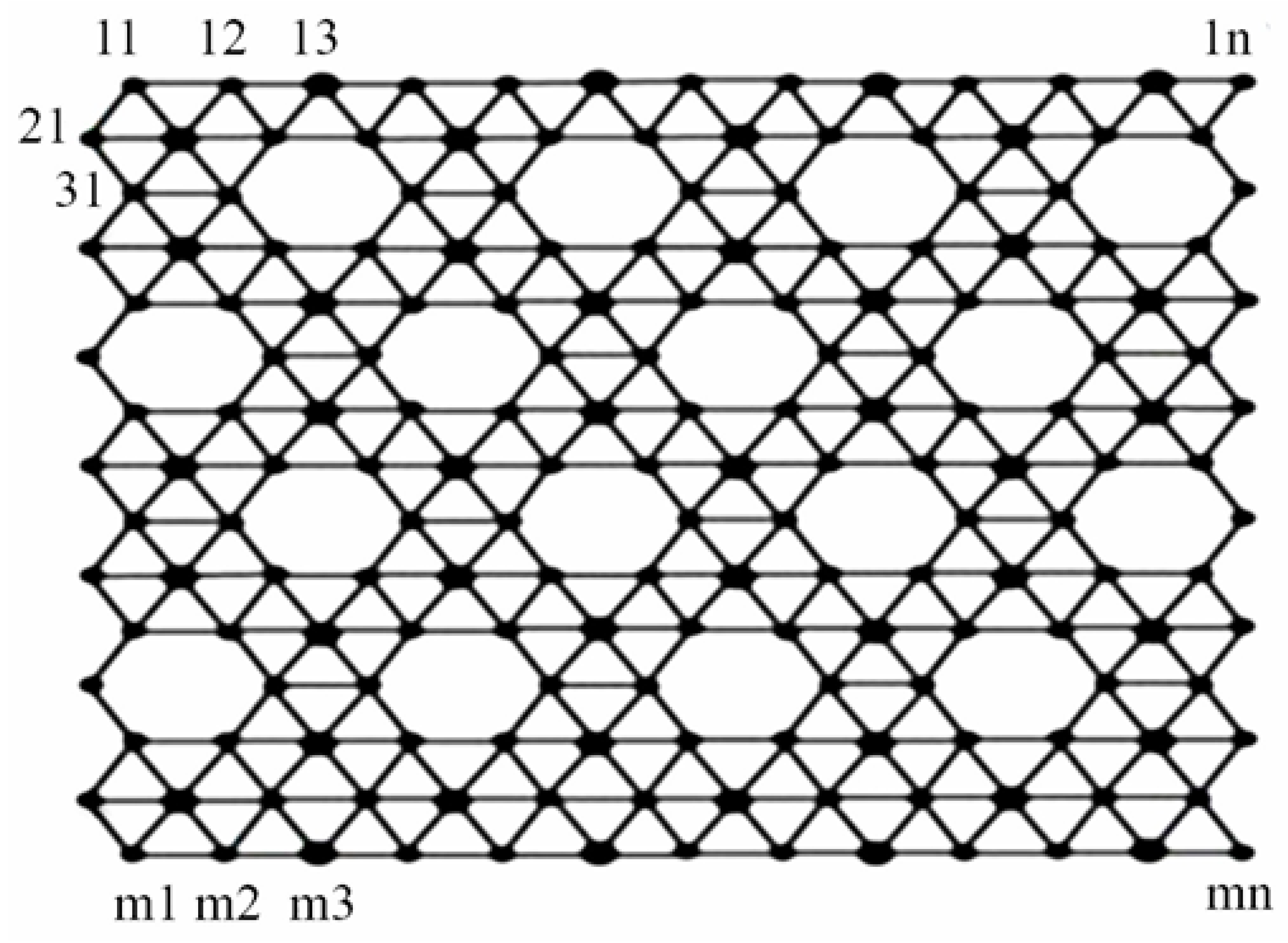
In the present article, we intend to compute the metric dimension of 2D lattices of an α-boron Nanotube. For the rest of this article, we reserve the symbol $T_{m,n}$ for the 2D lattice of the α-boron Nanotube of dimensions m and n. We use the term lattice only to denote the 2D sheet of the alpha-boron tubes. The vertices of the alpha-boron sheet in the first row are $u_{11},u_{12},u_{13},\dots ,u_{1n}$, in second row $u_{21},u_{22},\dots ,u_{2n}$, in third row $u_{31},u_{32},u_{34},u_{35},u_{37},u_{38}\dots ,u_{3n}$, etc. The representation of vertices is $u_{ij}$, where $i$ is the row number and $j$ is the column number. For the sake of simplicity, we label the vertices in Figure 2 as 11, 12, 13 etc. instead of $u_{11},u_{12},u_{13}$ etc. Please see below, Figure 2.

In the tubes, m1 and 1n are connected with each other, whereas in the 2D-lattice these vertices are at $n-1$ distance apart, see Figure 3.

2. Main Results

Theorem 1.

For all $m,n\in Z^{+}$ and $m<n$, we have $\dim (T_{m,n})=2$.

Proof. 

We consider the following labelling of vertices of 2D-lattice of alpha-boron tubes as depicted in the above figure. Consider $m\times n$ 2D-lattice of $\alpha -\mathrm{boron}$ nanotubes. The vertex set of G is partitioned as

$$\begin{gathered} \begin{array}{l}\{u_{11},u_{12},u_{13},\dots ,u_{1n},u_{21},u_{22},\dots ,u_{2n},u_{41},u_{42},\dots ,u_{4n},u_{51},u_{52},\dots ,u_{5n},u_{71},u_{72},\dots ,u_{7n},\dots ,u_{m1},u_{m2},\\ \dots ,u_{mn}\} \\ \cup \left\{u_{31},u_{32},u_{34},u_{35},u_{37},u_{38}\dots ,u_{3n},u_{61},u_{63},u_{64},u_{66},u_{67},u_{69},\dots ,u_{6n},u_{91},u_{92},u_{94},u_{95},u_{97},u_{98},\dots \dots ,u_{9n}\right\}\end{array} \end{gathered}$$

If m < n

Let $W=\left\{u_{11},u_{1n}\right\}$. We prove that $W$ is a resolving set for $T_{m,n}$. The representations of different vertices of $T_{m,n}$ are

$$Fori=1{,\mathrm{r}(\mathrm{u}}_{ij}|W)=\left(j-1,n-j\right);1\le j\le n$$

$$Fori=2{,\mathrm{r}(\mathrm{u}}_{ij}|W)=\{\begin{array}{l}\left(1,n\right);j=1\\ \left(j-1,n+1-j\right);2\le j\le n\end{array}$$

In general, for 3 < i ≤ m where i is odd and i ≠ 3k

$${\mathrm{r}(\mathrm{u}}_{ij}|W)=\{\begin{array}{ll}(i-1,n+\frac{i-1}{2}-j);& 1\le j\le \frac{i-1}{2}\\ (j+\frac{i-3}{2},n+\frac{i-1}{2}-j);& \frac{i+1}{2}\le j\le n-\frac{i-1}{2}\\ (j+\frac{i-3}{2},i-1);& n-\frac{i-3}{2}\le j\le n\end{array}$$

In general, for 4 ≤ i ≤ m where i is even and i ≠ 3k

$${\mathrm{r}(\mathrm{u}}_{ij}|W)=\{\begin{array}{ll}(i-1,n+\frac{i}{2}-j);& 1\le j\le \frac{i}{2}\\ (j+\frac{i-4}{2},n+\frac{i}{2}-j);& \frac{i+2}{2}\le j\le n-\frac{i-2}{2}\\ (j+\frac{i-4}{2},i-1);& n-\frac{i-4}{2}\le j\le n\end{array}$$

$\mathrm{For}i=3k,3k\mathrm{is}\mathrm{odd}\mathrm{and}j\ne 3\mathrm{p}$

$${\mathrm{r}(\mathrm{u}}_{ij}|W)=\{\begin{array}{ll}(i-1,n+\frac{i-1}{2}-j);& 1\le j\le \frac{i-1}{2}\\ (j+\frac{i-3}{2},n+\frac{i-1}{2}-j);& \frac{i+1}{2}\le j\le n-\frac{i-1}{2}\\ (j+\frac{i-3}{2},i-1);& n-\frac{i-3}{2}\le j\le n\end{array}$$

$\mathrm{For}i=3k,3k\mathrm{is}\mathrm{even}\mathrm{and}j\ne 3\mathrm{p}-1$

$${\mathrm{r}(\mathrm{u}}_{ij}|W)=\{\begin{array}{ll}(i-1,n+\frac{i}{2}-j);& 1\le j\le \frac{i}{2}\\ (j+\frac{i-4}{2},n+\frac{i}{2}-j);& \frac{i+2}{2}\le j\le n-\frac{i-2}{2}\\ (j+\frac{i-4}{2},i-1);& n-\frac{i-4}{2}\le j\le n\end{array}$$

These representations are distinct. So $W$ is a resolving set for $T_{m,n}$ and the dim($T_{m,n}$) ≤ 2. Since $T_{m,n}$ is not a path so dim($T_{m,n}$) ≥ 2. Hence the dim($T_{m,n}$) = 2 in this case. ☐

Theorem 2.

For all $m,n\in Z^{+}$ and $m\ge n$, we have $\dim (T_{m,n})\le 3,$

Proof. 

Let $W=\left\{u_{11},u_{1n},u_{m1}\right\}$. We prove that $W$ is a resolving set. The representations of vertices $u_{ij}$ with respect to W are

• Case I:m is odd with $n\le m<2n$ and m ≠ 6k + 1

  $$Fori=1{,\mathrm{r}(\mathrm{u}}_{ij}|W)=\{\begin{array}{l}\left(j-1,n-j,m-1\right);1\le j\le \frac{m+1}{2}\\ \left(j-1,n-j,j+\frac{m-3}{2}\right);\frac{m+3}{2}\le j\le n\end{array}$$

  $$Fori=2,{\mathrm{r}(\mathrm{u}}_{ij}|W)=\{\begin{array}{l}\left(1,n,m-2\right);j=1\\ \left(j-1,n+1-j,m-2\right);2\le j\le \frac{m+1}{2}\\ \left(j-1,n+1-j,j+\frac{m-5}{2}\right);\frac{m+3}{2}\le j\le n\end{array}$$
  If i is odd and i ≠ 3k then
  $\mathrm{for}3<i\le \lceil \frac{m}{2}\rceil$

  $${\mathrm{r}(\mathrm{u}}_{ij}|W)=\{\begin{array}{ll}(i-1,n+\lfloor \frac{i}{2}\rfloor -j,m-i);& 1\le j\le \frac{i-1}{2},\\ (j+\lfloor \frac{i-3}{2}\rfloor ,n+\lfloor \frac{i}{2}\rfloor -j,m-i);& \frac{i+1}{2}\le j\le \frac{m-(i-2)}{2},\\ (j+\lfloor \frac{i-3}{2}\rfloor ,n+\lfloor \frac{i}{2}\rfloor -j,j+\frac{m-(i+2)}{2});& \frac{m-(i-4)}{2}\le j\le n-\frac{i-1}{2}\\ (j+\lfloor \frac{i-3}{2}\rfloor ,i-1,j+\frac{m-(i+2)}{2});& n-\frac{i-3}{2}\le j\le n\end{array}$$
  $\mathrm{for}\lceil \frac{m}{2}\rceil +1\le i\le m$

  $${\mathrm{r}(\mathrm{u}}_{ij}|W)=\{\begin{array}{ll}(i-1,n+\lfloor \frac{i}{2}\rfloor -j,m-i);& 1\le j\le \frac{m-(i-2)}{2},\\ (i-1,n+\lfloor \frac{i}{2}\rfloor -j,j+\frac{m-(i+2)}{2});& \frac{m-(i-4)}{2}\le j\le \frac{i-1}{2},\\ (j+\lfloor \frac{i-3}{2}\rfloor ,n+\lfloor \frac{i}{2}\rfloor -j,j+\frac{m-(i+2)}{2});& \frac{i+1}{2}\le j\le n-\frac{i-1}{2}\\ (j+\lfloor \frac{i-3}{2}\rfloor ,i-1,j+\frac{m-(i+2)}{2});& n-\frac{i-3}{2}\le j\le n\end{array}$$
  If i is even and i ≠ 3k then
  $\mathrm{for}3<i\le \lceil \frac{m}{2}\rceil$

  $${\mathrm{r}(\mathrm{u}}_{ij}|W)=\{\begin{array}{ll}(i-1,n+\lfloor \frac{i}{2}\rfloor -j,m-i);& 1\le j\le \frac{i}{2},\\ (j+\lfloor \frac{i-3}{2}\rfloor ,n+\lfloor \frac{i}{2}\rfloor -j,m-i);& \frac{i+2}{2}\le j\le \frac{m-(i-3)}{2},\\ (j+\lfloor \frac{i-3}{2}\rfloor ,n+\lfloor \frac{i}{2}\rfloor -j,j+\frac{m-(i+3)}{2});& \frac{m-(i-5)}{2}\le j\le n-\frac{i-2}{2}\\ (j+\lfloor \frac{i-3}{2}\rfloor ,i-1,j+\frac{m-(i+3)}{2});& n-\frac{i-4}{2}\le j\le n\end{array}$$
  $\mathrm{for}\lceil \frac{m}{2}\rceil +1\le i\le m$

  $${\mathrm{r}(\mathrm{u}}_{ij}|W)=\{\begin{array}{ll}(i-1,n+\lfloor \frac{i}{2}\rfloor -j,m-i);& 1\le j\le \frac{m-(i-3)}{2},\\ (i-1,n+\lfloor \frac{i}{2}\rfloor -j,j+\frac{m-(i+3)}{2});& \frac{m-(i-5)}{2}\le j\le \frac{i}{2},\\ (j+\lfloor \frac{i-3}{2}\rfloor ,n+\lfloor \frac{i}{2}\rfloor -j,j+\frac{m-(i+3)}{2});& \frac{i+2}{2}\le j\le n-\frac{i-2}{2}\\ (j+\lfloor \frac{i-3}{2}\rfloor ,i-1,j+\frac{m-(i+3)}{2});& n-\frac{i-4}{2}\le j\le n\end{array}$$
  If m = 6k + 1 with i ≠ 3k and i is odd
  $\mathrm{for}3<i\le \lceil \frac{m}{2}\rceil$

  $${\mathrm{r}(\mathrm{u}}_{ij}|W)=\{\begin{array}{ll}(i-1,n+\lfloor \frac{i}{2}\rfloor -j,m-i);& 1\le j\le \frac{i-1}{2},\\ (j+\lfloor \frac{i-3}{2}\rfloor ,n+\lfloor \frac{i}{2}\rfloor -j,m-i);& \frac{i+1}{2}\le j\le \frac{m-i}{2},\\ (j+\lfloor \frac{i-3}{2}\rfloor ,n+\lfloor \frac{i}{2}\rfloor -j,m-i+1);& j=\frac{m-(i-2)}{2}\\ (j+\lfloor \frac{i-3}{2}\rfloor ,n+\lfloor \frac{i}{2}\rfloor -j,j+\frac{m-(i+2)}{2});& \frac{m-(i-4)}{2}\le j\le n-\frac{i-1}{2},\\ (j+\lfloor \frac{i-3}{2}\rfloor ,i-1,j+\frac{m-(i+2)}{2});& n-\frac{i-3}{2}\le j\le n,\end{array}$$
  $\mathrm{for}\lceil \frac{m}{2}\rceil +1\le i\le m$

  $${\mathrm{r}(\mathrm{u}}_{ij}|W)=\{\begin{array}{ll}(i-1,n+\lfloor \frac{i}{2}\rfloor -j,m-i);& 1\le j\le \frac{m-i}{2},\\ (i-1,n+\lfloor \frac{i}{2}\rfloor -j,m-i+1);& j=\frac{m-(i-2)}{2},\\ (i-1,n+\lfloor \frac{i}{2}\rfloor -j,j+\frac{m-(i+2)}{2});& \frac{m-(i-4)}{2}\le j\le \frac{i-1}{2}\\ (j+\lfloor \frac{i-3}{2}\rfloor ,n+\lfloor \frac{i}{2}\rfloor -j,j+\frac{m-(i+2)}{2});& \frac{i+1}{2}\le j\le n-\frac{i-1}{2},\\ (j+\lfloor \frac{i-3}{2}\rfloor ,i-1,j+\frac{m-(i+2)}{2});& n-\frac{i-3}{2}\le j\le n,\end{array}$$
  If m = 6k + 1 with i ≠ 3k and i is even
  $\mathrm{for}3<i\le \lceil \frac{m}{2}\rceil$

  $${\mathrm{r}(\mathrm{u}}_{ij}|W)=\{\begin{array}{ll}(i-1,n+\lfloor \frac{i}{2}\rfloor -j,m-i);& 1\le j\le \frac{i}{2},\\ (j+\lfloor \frac{i-3}{2}\rfloor ,n+\lfloor \frac{i}{2}\rfloor -j,m-i);& \frac{i+2}{2}\le j\le \frac{m-(i-1)}{2},\\ (j+\lfloor \frac{i-3}{2}\rfloor ,n+\lfloor \frac{i}{2}\rfloor -j,m-i+1);& j=\frac{m-(i-3)}{2}\\ (j+\lfloor \frac{i-3}{2}\rfloor ,n+\lfloor \frac{i}{2}\rfloor -j,j+\frac{m-(i+2)}{2});& \frac{m-(i-5)}{2}\le j\le n-\frac{i-2}{2},\\ (j+\lfloor \frac{i-3}{2}\rfloor ,i-1,j+\frac{m-(i+2)}{2});& n-\frac{i-4}{2}\le j\le n,\end{array}$$
  $\mathrm{for}\lceil \frac{m}{2}\rceil +1\le i\le m$

  $${\mathrm{r}(\mathrm{u}}_{ij}|W)=\{\begin{array}{ll}(i-1,n+\lfloor \frac{i}{2}\rfloor -j,m-i);& 1\le j\le \frac{m-(i-1)}{2},\\ (i-1,n+\lfloor \frac{i}{2}\rfloor -j,m-i+1);& j=\frac{m-(i-3)}{2},\\ (i-1,n+\lfloor \frac{i}{2}\rfloor -j,j+\frac{m-(i+2)}{2});& \frac{m-(i-5)}{2}\le j\le \frac{i}{2}\\ (j+\lfloor \frac{i-3}{2}\rfloor ,n+\lfloor \frac{i}{2}\rfloor -j,j+\frac{m-(i+2)}{2});& \frac{i+2}{2}\le j\le n-\frac{i-2}{2},\\ (j+\lfloor \frac{i-3}{2}\rfloor ,i-1,j+\frac{m-(i+2)}{2});& n-\frac{i-4}{2}\le j\le n,\end{array}$$
  If $i=3k$ and $3k$ is odd
  $\mathrm{for}3<i\le \lceil \frac{m}{2}\rceil$

  $${\mathrm{r}(\mathrm{u}}_{ij}|W)=\{\begin{array}{ll}(i-1,n+\lfloor \frac{i}{2}\rfloor -j,m-i);& 1\le j\le \frac{i-1}{2},j\ne 3l\\ (j+\lfloor \frac{i-3}{2}\rfloor ,n+\lfloor \frac{i}{2}\rfloor -j,m-i);& \frac{i+1}{2}\le j\le \frac{m-(i-2)}{2},j\ne 3l\\ (j+\lfloor \frac{i-3}{2}\rfloor ,n+\lfloor \frac{i}{2}\rfloor -j,j+\frac{m-(i+2)}{2});& \frac{m-(i-4)}{2}\le j\le n-\frac{i-1}{2},j\ne 3l\\ (j+\lfloor \frac{i-3}{2}\rfloor ,i-1,j+\frac{m-(i+2)}{2});& n-\frac{i-3}{2}\le j\le n,j\ne 3l\end{array}$$
  $\mathrm{for}\lceil \frac{m}{2}\rceil +1\le i\le m$

  $${\mathrm{r}(\mathrm{u}}_{ij}|W)=\{\begin{array}{ll}(i-1,n+\lfloor \frac{i}{2}\rfloor -j,m-i);& 1\le j\le \frac{m-(i-2)}{2},j\ne 3l\\ (i-1,n+\lfloor \frac{i}{2}\rfloor -j,j+\frac{m-(i+2)}{2});& \frac{m-(i-4)}{2}\le j\le \frac{i-1}{2},j\ne 3l\\ (j+\lfloor \frac{i-3}{2}\rfloor ,n+\lfloor \frac{i}{2}\rfloor -j,j+\frac{m-(i+2)}{2});& \frac{i+1}{2}\le j\le n-\frac{i-1}{2},j\ne 3l\\ (j+\lfloor \frac{i-3}{2}\rfloor ,i-1,j+\frac{m-(i+2)}{2});& n-\frac{i-3}{2}\le j\le n,j\ne 3l\end{array}$$
  If $i=3k$ and $3k$ is even
  $\mathrm{for}3<i\le \lceil \frac{m}{2}\rceil$

  $${\mathrm{r}(\mathrm{u}}_{ij}|W)=\{\begin{array}{ll}(i-1,n+\lfloor \frac{i}{2}\rfloor -j,m-i);& 1\le j\le \frac{i}{2},j\ne 3l-1\\ (j+\lfloor \frac{i-3}{2}\rfloor ,n+\lfloor \frac{i}{2}\rfloor -j,m-i);& \frac{i+2}{2}\le j\le \frac{m-(i-3)}{2},j\ne 3l-1\\ (j+\lfloor \frac{i-3}{2}\rfloor ,n+\lfloor \frac{i}{2}\rfloor -j,j+\frac{m-(i+3)}{2});& \frac{m-(i-5)}{2}\le j\le n-\frac{i-2}{2},j\ne 3l-1\\ (j+\lfloor \frac{i-3}{2}\rfloor ,i-1,j+\frac{m-(i+3)}{2});& n-\frac{i-4}{2}\le j\le n,j\ne 3l-1\end{array}$$
  $\mathrm{for}\lceil \frac{m}{2}\rceil +1\le i\le m$

  $${\mathrm{r}(\mathrm{u}}_{ij}|W)=\{\begin{array}{ll}(i-1,n+\lfloor \frac{i}{2}\rfloor -j,m-i);& 1\le j\le \frac{m-(i-3)}{2},j\ne 3l-1\\ (i-1,n+\lfloor \frac{i}{2}\rfloor -j,j+\frac{m-(i+3)}{2});& \frac{m-(i-5)}{2}\le j\le \frac{i}{2},j\ne 3l-1\\ (j+\lfloor \frac{i-3}{2}\rfloor ,n+\lfloor \frac{i}{2}\rfloor -j,j+\frac{m-(i+3)}{2});& \frac{i+2}{2}\le j\le n-\frac{i-2}{2},j\ne 3l-1\\ (j+\lfloor \frac{i-3}{2}\rfloor ,i-1,j+\frac{m-(i+3)}{2});& n-\frac{i-4}{2}\le j\le n,j\ne 3l-1\end{array}$$
• Case II: If $m$ is even and $m\ne 6k+2$
  For i is odd and $i\ne 3k$
  $\mathrm{for}3<i\le \lceil \frac{m}{2}\rceil$

  $${\mathrm{r}(\mathrm{u}}_{ij}|W)=\{\begin{array}{ll}(i-1,n+\lfloor \frac{i}{2}\rfloor -j,m-i);& 1\le j\le \frac{i-1}{2},\\ (j+\lfloor \frac{i-3}{2}\rfloor ,n+\lfloor \frac{i}{2}\rfloor -j,m-i);& \frac{i+1}{2}\le j\le \frac{m-(i-1)}{2},\\ (j+\lfloor \frac{i-3}{2}\rfloor ,n+\lfloor \frac{i}{2}\rfloor -j,j+\frac{m-(i+1)}{2});& \frac{m-(i-3)}{2}\le j\le n-\frac{i-1}{2}\\ (j+\lfloor \frac{i-3}{2}\rfloor ,i-1,j+\frac{m-(i+1)}{2});& n-\frac{i-3}{2}\le j\le n\end{array}$$
  $\mathrm{for}\lceil \frac{m}{2}\rceil +1\le i\le m$

  $${\mathrm{r}(\mathrm{u}}_{ij}|W)=\{\begin{array}{ll}(i-1,n+\lfloor \frac{i}{2}\rfloor -j,m-i);& 1\le j\le \frac{m-(i-1)}{2},\\ (i-1,n+\lfloor \frac{i}{2}\rfloor -j,j+\frac{m-(i+1)}{2});& \frac{m-(i-3)}{2}\le j\le \frac{i-1}{2},\\ (j+\lfloor \frac{i-3}{2}\rfloor ,n+\lfloor \frac{i}{2}\rfloor -j,j+\frac{m-(i+1)}{2});& \frac{i+1}{2}\le j\le n-\frac{i-1}{2}\\ (j+\lfloor \frac{i-3}{2}\rfloor ,i-1,j+\frac{m-(i+1)}{2});& n-\frac{i-3}{2}\le j\le n\end{array}$$
  If $i$ is even $i\ne 3k$
  $\mathrm{for}3<i\le \lceil \frac{m}{2}\rceil$

  $${\mathrm{r}(\mathrm{u}}_{ij}|W)=\{\begin{array}{ll}(i-1,n+\lfloor \frac{i}{2}\rfloor -j,m-i);& 1\le j\le \frac{i}{2},\\ (j+\lfloor \frac{i-3}{2}\rfloor ,n+\lfloor \frac{i}{2}\rfloor -j,m-i);& \frac{i+2}{2}\le j\le \frac{m-(i-2)}{2},\\ (j+\lfloor \frac{i-3}{2}\rfloor ,n+\lfloor \frac{i}{2}\rfloor -j,j+\frac{m-(i+2)}{2});& \frac{m-(i-4)}{2}\le j\le n-\frac{i-2}{2}\\ (j+\lfloor \frac{i-3}{2}\rfloor ,i-1,j+\frac{m-(i+2)}{2});& n-\frac{i-4}{2}\le j\le n\end{array}$$
  $\mathrm{for}\lceil \frac{m}{2}\rceil +1\le i\le m$

  $${\mathrm{r}(\mathrm{u}}_{ij}|W)=\{\begin{array}{ll}(i-1,n+\lfloor \frac{i}{2}\rfloor -j,m-i);& 1\le j\le \frac{m-(i-2)}{2},\\ (i-1,n+\lfloor \frac{i}{2}\rfloor -j,j+\frac{m-(i+2)}{2});& \frac{m-(i-4)}{2}\le j\le \frac{i}{2},\\ (j+\lfloor \frac{i-3}{2}\rfloor ,n+\lfloor \frac{i}{2}\rfloor -j,j+\frac{m-(i+2)}{2});& \frac{i+2}{2}\le j\le n-\frac{i-2}{2}\\ (j+\lfloor \frac{i-3}{2}\rfloor ,i-1,j+\frac{m-(i+2)}{2});& n-\frac{i-4}{2}\le j\le n\end{array}$$
  If $m=6k+2$ with $i\ne 3k$ and $i$ is odd
  $\mathrm{for}3<i\le \lceil \frac{m}{2}\rceil$

  $${\mathrm{r}(\mathrm{u}}_{ij}|W)=\{\begin{array}{ll}(i-1,n+\lfloor \frac{i}{2}\rfloor -j,m-i);& 1\le j\le \frac{i-3}{2},\\ (j+\lfloor \frac{i-3}{2}\rfloor ,n+\lfloor \frac{i}{2}\rfloor -j,m-i);& \frac{i-1}{2}\le j\le \frac{m-(i+1)}{2},\\ (j+\lfloor \frac{i-3}{2}\rfloor ,n+\lfloor \frac{i}{2}\rfloor -j,m-i+1);& j=\frac{m-(i-1)}{2}\\ (j+\lfloor \frac{i-3}{2}\rfloor ,n+\lfloor \frac{i}{2}\rfloor -j,j+\frac{m-(i+2)}{2});& \frac{m-(i-3)}{2}\le j\le n-\frac{i-1}{2},\\ (j+\lfloor \frac{i-3}{2}\rfloor ,i-1,j+\frac{m-(i+2)}{2});& n-\frac{i-3}{2}\le j\le n,\end{array}$$
  $\mathrm{for}\lceil \frac{m}{2}\rceil +1\le i\le m$

  $${\mathrm{r}(\mathrm{u}}_{ij}|W)=\{\begin{array}{ll}(i-1,n+\lfloor \frac{i}{2}\rfloor -j,m-i);& 1\le j\le \frac{m-(i+1)}{2},\\ (i-1,n+\lfloor \frac{i}{2}\rfloor -j,m-i+1));& j=\frac{m-(i-1)}{2},\\ (i-1,n+\lfloor \frac{i}{2}\rfloor -j,j+\frac{m-(i+2)}{2});& \frac{m-(i-3)}{2}\le j\le \frac{i-3}{2},\\ (j+\lfloor \frac{i-3}{2}\rfloor ,n+\lfloor \frac{i}{2}\rfloor -j,j+\frac{m-(i+2)}{2});& \frac{i-1}{2}\le j\le n-\frac{i-1}{2},\\ (j+\lfloor \frac{i-3}{2}\rfloor ,i-1,j+\frac{m-(i+2)}{2});& n-\frac{i-3}{2}\le j\le n,\end{array}$$
  If $m=6k+2$ with $i\ne 3k$ and $i$ is even
  $\mathrm{for}3<i\le \lceil \frac{m}{2}\rceil$

  $${\mathrm{r}(\mathrm{u}}_{ij}|W)=\{\begin{array}{ll}(i-1,n+\lfloor \frac{i}{2}\rfloor -j,m-i);& 1\le j\le \frac{i}{2},\\ (j+\lfloor \frac{i-3}{2}\rfloor ,n+\lfloor \frac{i}{2}\rfloor -j,m-i);& \frac{i+2}{2}\le j\le \frac{m-i}{2},\\ (j+\lfloor \frac{i-3}{2}\rfloor ,n+\lfloor \frac{i}{2}\rfloor -j,m-i+1);& j=\frac{m-(i-2)}{2}\\ (j+\lfloor \frac{i-3}{2}\rfloor ,n+\lfloor \frac{i}{2}\rfloor -j,j+\frac{m-(i+2)}{2});& \frac{m-(i-4)}{2}\le j\le n-\frac{i-2}{2},\\ (j+\lfloor \frac{i-3}{2}\rfloor ,i-1,j+\frac{m-(i+2)}{2});& n-\frac{i-4}{2}\le j\le n,\end{array}$$
  $\mathrm{for}\lceil \frac{m}{2}\rceil +1\le i\le m$

  $${\mathrm{r}(\mathrm{u}}_{ij}|W)=\{\begin{array}{ll}(i-1,n+\lfloor \frac{i}{2}\rfloor -j,m-i);& 1\le j\le \frac{m-i}{2},\\ (i-1,n+\lfloor \frac{i}{2}\rfloor -j,m-i+1);& j=\frac{m-(i-2)}{2},\\ (i-1,n+\lfloor \frac{i}{2}\rfloor -j,j+\frac{m-(i+2)}{2});& \frac{m-(i-4)}{2}\le j\le \frac{i-2}{2},\\ (j+\lfloor \frac{i-3}{2}\rfloor ,n+\lfloor \frac{i}{2}\rfloor -j,j+\frac{m-(i+2)}{2});& \frac{i}{2}\le j\le n-\frac{i-2}{2},\\ (j+\lfloor \frac{i-3}{2}\rfloor ,i-1,j+\frac{m-(i+2)}{2});& n-\frac{i-4}{2}\le j\le n,\end{array}$$
  If $i=3k$ and $3k$ is odd
  $\mathrm{for}3<i\le \lceil \frac{m}{2}\rceil$

  $${\mathrm{r}(\mathrm{u}}_{ij}|W)=\{\begin{array}{ll}(i-1,n+\lfloor \frac{i}{2}\rfloor -j,m-i);& 1\le j\le \frac{i-1}{2},j\ne 3k\\ (j+\lfloor \frac{i-3}{2}\rfloor ,n+\lfloor \frac{i}{2}\rfloor -j,m-i);& \frac{i+1}{2}\le j\le \frac{m-(i-2)}{2},j\ne 3k\\ (j+\lfloor \frac{i-3}{2}\rfloor ,n+\lfloor \frac{i}{2}\rfloor -j,j+\frac{m-(i+2)}{2});& \frac{m-(i-4)}{2}\le j\le n-\frac{i-1}{2},j\ne 3k\\ (j+\lfloor \frac{i-3}{2}\rfloor ,i-1,j+\frac{m-(i+2)}{2});& n-\frac{i-3}{2}\le j\le n,j\ne 3k\end{array}$$
  $\mathrm{for}\lceil \frac{m}{2}\rceil +1\le i\le m$

  $${\mathrm{r}(\mathrm{u}}_{ij}|W)=\{\begin{array}{ll}(i-1,n+\lfloor \frac{i}{2}\rfloor -j,m-i);& 1\le j\le \frac{m-(i-2)}{2},j\ne 3k\\ (i-1,n+\lfloor \frac{i}{2}\rfloor -j,j+\frac{m-(i+2)}{2});& \frac{m-(i-4)}{2}\le j\le \frac{i-1}{2},j\ne 3k\\ (j+\lfloor \frac{i-3}{2}\rfloor ,n+\lfloor \frac{i}{2}\rfloor -j,j+\frac{m-(i+2)}{2});& \frac{i+1}{2}\le j\le n-\frac{i-1}{2},j\ne 3k\\ (j+\lfloor \frac{i-3}{2}\rfloor ,i-1,j+\frac{m-(i+2)}{2});& n-\frac{i-3}{2}\le j\le n,j\ne 3k\end{array}$$
  If $i=3k$ and $3k$ is odd
  $\mathrm{for}3<i\le \lceil \frac{m}{2}\rceil$

  $${\mathrm{r}(\mathrm{u}}_{ij}|W)=\{\begin{array}{ll}(i-1,n+\lfloor \frac{i}{2}\rfloor -j,m-i);& 1\le j\le \frac{i}{2},j\ne 3k-1\\ (j+\lfloor \frac{i-3}{2}\rfloor ,n+\lfloor \frac{i}{2}\rfloor -j,m-i);& \frac{i+2}{2}\le j\le \frac{m-(i-3)}{2},j\ne 3k-1\\ (j+\lfloor \frac{i-3}{2}\rfloor ,n+\lfloor \frac{i}{2}\rfloor -j,j+\frac{m-(i+3)}{2});& \frac{m-(i-5)}{2}\le j\le n-\frac{i-2}{2},j\ne 3k-1\\ (j+\lfloor \frac{i-3}{2}\rfloor ,i-1,j+\frac{m-(i+3)}{2});& n-\frac{i-4}{2}\le j\le n,j\ne 3k-1\end{array}$$
  $\mathrm{for}\lceil \frac{m}{2}\rceil +1\le i\le m$

  $$r(u_{ij}|W)=\{\begin{array}{ll}(i-1,n+\lfloor \frac{i}{2}\rfloor -j,m-i);& 1\le j\le \frac{m-(i-3)}{2},j\ne 3k-1\\ (i-1,n+\lfloor \frac{i}{2}\rfloor -j,j+\frac{m-(i+3)}{2});& \frac{m-(i-5)}{2}\le j\le \frac{i}{2},j\ne 3k-1\\ (j+\lfloor \frac{i-3}{2}\rfloor ,n+\lfloor \frac{i}{2}\rfloor -j,j+\frac{m-(i+3)}{2});& \frac{i+2}{2}\le j\le n-\frac{i-2}{2},j\ne 3k-1\\ (j+\lfloor \frac{i-3}{2}\rfloor ,i-1,j+\frac{m-(i+3)}{2});& n-\frac{i-4}{2}\le j\le n,j\ne 3k-1\end{array}$$
  $Fori=2n-1,r(u_{ij}|W)=(2n-2,2n-2,j-1);1\le j\le n$
  $Fori=2n-2,r(u_{ij}|W)=\{\begin{array}{ll}\left(2n-3,2n-2,1\right);& j=1\\ \left(2n-3,2n-3,j-1\right);& 2\le j\le n\end{array}$
  If m is odd, $r\ge 2$ and $rn\le m<(r+1)n$
  For i = rn + k where $0\le k\le n-1$
  If $i$ is odd,

  $$r(u_{ij}|W)=\{\begin{array}{ll}\left(rn+k-1,rn+k-1,m-i\right);& 1\le j\le \frac{m-(rn+k-2)}{2}\\ \left(rn+k-1,rn+k-1,j+\frac{m-(rn+k+2)}{2}\right);& \frac{m-(rn+k-4)}{2}\le j\le n\end{array}$$
  If $i$ is even,

  $$r(u_{ij}|W)=\{\begin{array}{ll}\left(rn+k-1,rn+k-1,m-i\right);& 1\le j\le \frac{m-(rn+k-3)}{2}\\ \left(rn+k-1,rn+k-1,j+\frac{m-(rn+k+3)}{2}\right);& \frac{m-(rn+k-5)}{2}\le j\le n\end{array}$$
  If $i=3k,i\mathrm{is}\mathrm{odd}\mathrm{and}j\ne 3p\mathrm{then}$

  $$r(u_{ij}|W)=\{\begin{array}{ll}\left(rn+k-1,rn+k-1,m-i\right);& 1\le j\le \frac{m-(rn+k-2)}{2}\\ \left(rn+k-1,rn+k-1,j+\frac{m-(rn+k+2)}{2}\right);& \frac{m-(rn+k-4)}{2}\le j\le n\end{array}$$
  $\mathrm{If}i=3k,i\mathrm{is}\mathrm{even}\mathrm{and}j\ne 3p-1\mathrm{then}$

  $$r(u_{ij}|W)=\{\begin{array}{ll}\left(rn+k-1,rn+k-1,m-i\right);& 1\le j\le \frac{m-(rn+k-3)}{2}\\ \left(rn+k-1,rn+k-1,j+\frac{m-(rn+k+3)}{2}\right);& \frac{m-(rn+k-5)}{2}\le j\le n\end{array}$$
  If m is even, $r\ge 2$ and $rn\le m<(r+1)n$
  For i = rn + k where $0\le k\le n-1$
  If i is odd,

  $$r(u_{ij}|W)=\{\begin{array}{ll}\left(rn+k-1,rn+k-1,m-i\right);& 1\le j\le \frac{m-(rn+k-1)}{2}\\ \left(rn+k-1,rn+k-1,j+\frac{m-(rn+k+1)}{2}\right);& \frac{m-(rn+k-3)}{2}\le j\le n\end{array}$$
  If i is even,

  $$r(u_{ij}|W)=\{\begin{array}{ll}\left(rn+k-1,rn+k-1,m-i\right);& 1\le j\le \frac{m-(rn+k-2)}{2}\\ \left(rn+k-1,rn+k-1,j+\frac{m-(rn+k+2)}{2}\right);& \frac{m-(rn+k-4)}{2}\le j\le n\end{array}$$
  $\mathrm{If}i=3k,i\mathrm{is}\mathrm{odd}\mathrm{and}j\ne 3p\mathrm{then}$

  $$r(u_{ij}|W)=\{\begin{array}{ll}\left(rn+k-1,rn+k-1,m-i\right);& 1\le j\le \frac{m-(rn+k-1)}{2}\\ \left(rn+k-1,rn+k-1,j+\frac{m-(rn+k+1)}{2}\right);& \frac{m-(rn+k-3)}{2}\le j\le n\end{array}$$
  $\mathrm{If}i=3k,i\mathrm{is}\mathrm{even}\mathrm{and}j\ne 3p-1\mathrm{then}$

  $$r(u_{ij}|W)=\{\begin{array}{ll}\left(rn+k-1,rn+k-1,m-i\right);& 1\le j\le \frac{m-(rn+k-2)}{2}\\ \left(rn+k-1,rn+k-1,j+\frac{m-(rn+k+2)}{2}\right);& \frac{m-(rn+k-4)}{2}\le j\le n\end{array}$$

These representations are distinct. So, $W$ is a resolving set for $T_{m,n}$. Therefore, the metric dimension of $T_{m,n}$ is ≤3. Now we prove that the metric dimension of $T_{m,n}$ is greater than 2. For this we shall prove that any set of cardinality two does not resolve. ☐

Theorem 3.

For all $m,n\in Z^{+}$ and $m\ge n$, we have $\dim (T_{m,n})\ge 3,$

Proof. 

Let $W=\left\{u_{ij},u_{pq}\right\}$ be a resolving set for $T_{m,n}$. We consider all possibilities and come up with a contradistinction in each case. The following three possibilities arise

Possibility 1: If $u_{ij},u_{pq}$ lie on the same row then i = p.

If $W=\left\{u_{11},u_{1n}\right\}$ then $r(u_{n+1,\frac{n}{2}}{|W)=r(u}_{n+1,\frac{n+2}{2}}|W)$ if n is even and $r(u_{n+1,\frac{n+1}{2}}{|W)=r(u}_{n+1,\frac{n+3}{2}}|W)$, if n is odd so both cases result in contradiction. In all remaining possibilities, we denote $u_x$ instead of $r(u_x|W)$ where no confusion arises.

(i)

If $W=\left\{u_{ij},u_{iq}\right\}$ and $1\le i<m$ and $1\le j<q<n$ then $u_{i,q+1}{=u}_{i+1,q+1}$, a contradiction.

(ii)

If $W=\left\{u_{ij},u_{iq}\right\}$ and $1\le i<m$, i = 3k and $1\le j<q<n$ then $u_{i-1,j}{=u}_{i+1,j}$ or $u_{i-1,j-1}{=u}_{i+1,j-1}$, a contradiction.

(iii)

If $W=\left\{u_{ij},u_{iq}\right\}$ and $1\le i<m$ and $1<j<q=n$ then $u_{i,j-1}{=u}_{i+1,j}$, a contradiction.

(iv)

If $W=\left\{u_{mj},u_{mq}\right\}$ and $1\le j<q<n$ then $u_{m,q+1}{=u}_{m-1,q}$ or $u_{m,q+1}{=u}_{m-1,q+1}$, a contradiction.

(v)

If $W=\left\{u_{mj},u_{mq}\right\}$ and $1<j<q=n$ then $u_{m,j-1}{=u}_{m-1,j}$, a contradiction.

(vi)

If $W=\left\{u_{i1},u_{in}\right\}$ and $1<i<m$ then $u_{i-1,1}{=u}_{i+1,1}$, a contradiction.

(vii)

If $W=\left\{u_{m1},u_{mn}\right\}$ and then $u_{m-n,3}{=u}_{m-n,4}$, a contradiction.

Possibility 2: If $u_{ij},u_{pq}$ lie on the same column then j = q.

(i)

If $W=\left\{u_{11},u_{m1}\right\}$ then $u_{21}{=u}_{22}$, a contradiction.

(ii)

If $W=\left\{u_{i1},u_{j1}\right\}$ and $1\le i<j<m$ then $u_{j3}{=u}_{j+1,3}$ or $u_{j3}{=u}_{j+1,2}$, a contradiction.

(iii)

If $W=\left\{u_{i1},u_{j1}\right\}$ and $1<i<j=m$ then $u_{i3}{=u}_{i-1,2}$ or $u_{i3}{=u}_{i-1,3}$, a contradiction.

(iv)

If $W=\left\{u_{iq},u_{jq}\right\}$, $1\le i<j<m\mathrm{and}1<q<n$ then $u_{j+1,q}{=u}_{j+1,q+1}$ or $u_{j+1,q}=u_{j+1,q-1}$, a contradiction.

(v)

If $W=\left\{u_{iq},u_{jq}\right\}$, $1<i<j\le m\mathrm{and}1<q<n$ then $u_{i-1,j-1}{=u}_{i-1,j}$ or $u_{i-1,j}{=u}_{i-1,j+1}$, a contradiction.

(vi)

If $W=\left\{u_{iq},u_{jq}\right\}$, $i=1,j=m\mathrm{and}1<q<n$ then $u_{2,j}=u_{2,j+1}$, a contradiction.

(vii)

If $W=\left\{u_{i,n-1},u_{j,n-1}\right\}$ and $i<j<m$ then $u_{j,n-2}{=u}_{j+1,n-2}$ or $u_{j,n-3}{=u}_{j+1,n-2}$, a contradiction.

(viii)

If $W=\left\{u_{1,n},u_{m,n}\right\}$ then either $u_{m-1,n-1}{=u}_{m-1,n}$ or $u_{m-2,n-1}{=u}_{m-2,n}$, a contradiction.

Possibility 3: If $u_{ij},u_{pq}$ lie neither on the same row nor the same column so i $\ne$ p and j $\ne$ q.

Let $W=\left\{u_{i,j},u_{p,q}\right\}$. Since i $\ne$ p so let i < p.

(i)

If j < q then $u_{p,q+1}{=u}_{p+1,q+1}$ or $u_{p,q+1}{=u}_{p+1,q}$, a contradiction

(ii)

If j > q then $u_{p-1,q}{=u}_{p,q+1}$ or $u_{p-1,q+1}{=u}_{p,q+1}$, a contradiction

(iii)

If i = 1 and p = m then $u_{2,j}=u_{2,j+1}$ or $u_{1,j+1}=u_{2,j+1}$ or $u_{m-1,q+1}=u_{m,q-1}$, a contradiction.

So any set with cardinality 2 does not resolve $T_{m,n}$. So, the metric dimension of $T_{m,n}$ is greater than 2. Hence metric dimension of $T_{m,n}$ is 3 if m > n. ☐

3. Conclusions and Discussion

In the present article, we computed the metric dimension of a 2D-lattice of alpha-boron nanotubes, $T_{m,n}$, and have come up with the following summarized result:

$$\dim \left(T_{m,n}\right)=\{\begin{array}{l}2\mathrm{if}m<n\\ 3\mathrm{if}m\ge n\end{array}$$

It is evident that the dimension depends upon the size of the 2D sheet. These results have applications in drug design, networking communication, robot navigations, designing new nano-devices and nano-engineering. Actually, these results are useful for engineer and hardware-designers that use alpha-boron sheets in different industries. It is overwhelming that they can capture the whole sheet uniquely if they know the resolving set and metric dimension. It can save time and cost if they choose only two or three vertices depending upon the size of the sheet using our results. We can conclude that every atom in the 2D sheet of alpha-boron nanotubes can be uniquely accessed and controlled by its metric basis whose cardinality is 2 or 3 depending upon the dimensions of the sheet.

References

- Manuel, P. Computational Aspects of Carbon and Boron Nanotubes. Molecules 2010, 15, 8709–8722. [Google Scholar] [CrossRef] [PubMed] [Green Version]
- Khuller, S.; Raghavachari, B.; Rosenfeld, A. Landmarks in graphs. Discret. Appl. Math. 1996, 70, 217–229. [Google Scholar] [CrossRef]
- Chartrand, G.; Poisson, C.; Zhang, P. Resolvability and the upper dimension of graphs. Comput. Math. Appl. 2000, 39, 19–28. [Google Scholar] [CrossRef]
- Bezugly, V.; Kunstmann, J.; Grundkötter-Stock, B.; Frauenheim, T.; Niehaus, T.; Cuniberti, G. Highly Conductive Boron Nanotubes: Transport Properties, Work Functions, and Structural Stabilities. ACS Nano 2011, 5, 4997–5005. [Google Scholar] [CrossRef] [PubMed]
- Cameron, P.; Lint, J. Designs, Graphs, Codes and Their Links, London Mathematical Society Student Texts; Cambridge University Press: Cambridge, UK, 1991; Volume 22. [Google Scholar]
- Deistal, R. Graph Theory; GTM 173; Springer: Berlin, Germany, 2017; ISBN 978-3-662-53621-6. [Google Scholar]
- Caceres, J.; Hernando, C.; Mora, M.; Pelayo, I.M.; Puertas, M.J.; Seara, C.; Wood, D.R. On the metric dimension of cartesian product of graphs. SIAM J. Discret. Math. 2007, 2, 423–441. [Google Scholar] [CrossRef]
- Buczkowski, P.S.; Chartrand, G.; Poisson, C.; Zhang, P. On k-dimensional graphs and their bases. Period. Math. Hung. 2003, 46, 9–15. [Google Scholar] [CrossRef]
- Imran, M.; Baig, A.Q.; Shafiq, M.K.; Tomescu, I. On the metric dimension of generalized Petersen graphs P(n, 3). Ars Comb. 2014, 117, 113–130. [Google Scholar]
- Chartrand, G.; Eroh, L.; Johnson, M.A.; Oellermann, O.R. Resolvability in graphs and the metric dimension of a graph. Discret. Appl. Math. 2000, 105, 99–113. [Google Scholar] [CrossRef]
- Harary, F.; Melter, R.A. On the metric dimension of a graph. Ars Comb. 1976, 2, 191–195. [Google Scholar]
- Slater, P.J. Leaves of trees. Congr. Numer. 1975, 14, 549–559. [Google Scholar]
- Sebő, A.; Tannier, E. On metric generators of graphs. Math. Oper. Res. 2004, 29, 383–393. [Google Scholar] [CrossRef]
- Chvatal, V. Mastermind. Combinatorica 1983, 3, 325–329. [Google Scholar] [CrossRef]
- Hernando, C.; Mora, M.; Pelayo, I.M.; Seara, C.; Caceres, J.; Puertas, M.L. On the metric dimension of some families of graphs. Electron. Notes Discret. Math. 2005, 22, 129–133. [Google Scholar] [CrossRef]
- Javaid, I.; Rahim, M.T.; Ali, K. Families of regular graphs with constant metric dimension. Util. Math. 2008, 75, 21–34. [Google Scholar]
- Ali, M.; Ali, G.; Imran, M.; Baig, A.Q.; Shafiq, M.K. On the metric dimension of Mobius ladders. Ars Comb. 2012, 105, 403–410. [Google Scholar]
- Munir, M.; Nizami, A.R.; Saeed, H. On the metric dimension of Möbius Ladder. Ars Comb. 2017, 135, 249–256. [Google Scholar]
- Siddique, H.M.A.; Imran, M. Computing the metric dimension of wheel related graphs. Appl. Math. Comput. 2014, 242, 624–632. [Google Scholar]
- Imran, S.; Siddiqui, M.K.; Imran, M.; Hussain, M.; Bilal, H.M.; Cheema, I.Z.; Tabraiz, A.; Saleem, Z. Computing the Metric Dimension of Gear Graphs. Symmetry 2018, 10, 209. [Google Scholar] [CrossRef]
- Manuel, P.; Rajan, B.; Rajasingh, I.; Monica, C. On minimum metric dimension of honeycomb networks. J. Discret. Algorithms 2008, 6, 20–27. [Google Scholar] [CrossRef]
- Imran, M.; Baig, A.Q.; Bokhary, S.A.; Javaid, I. On the metric dimension of circulant graphs. Appl. Math. Lett. 2012, 25, 320–325. [Google Scholar] [CrossRef]
- Baca, M.; Baskoro, E.T.; Salman, A.N.M.; Saputro, S.W.; Suprijanto, D. On metric dimension of regular bipartite graphs. Bull. Math. Soc. Sci. Math. Roum. 2011, 54, 15–28. [Google Scholar]
- Tomescu, I.; Javaid, I. On the metric dimension of the Jahangir graph. Bull. Math. Soc. Sci. Math. Roum. 2007, 50, 371–376. [Google Scholar]
- Grigorious, C.; Manuel, P.; Miller, M.; Rajan, B.; Stephen, S. On the metric dimension of circulant and Harary graphs. Appl. Math. Comput. 2014, 248, 47–54. [Google Scholar] [CrossRef]
Figure 1.
(a) 2D lattice of Triangular Boron Tubes; (b) 2D-lattice of alpha-boron Tubes.
Figure 2.
Alpha boron sheet.
Figure 3.
Alpha-boron nanotubes. (a) Sheet view and (b) tube view.
© 2018 by the authors. Licensee MDPI, Basel, Switzerland. This article is an open access article distributed under the terms and conditions of the Creative Commons Attribution (CC BY) license (http://creativecommons.org/licenses/by/4.0/).
Share and Cite
MDPI and ACS Style
Hussain, Z.; Munir, M.; Chaudhary, M.; Kang, S.M. Computing Metric Dimension and Metric Basis of 2D Lattice of Alpha-Boron Nanotubes. Symmetry 2018, 10, 300. https://doi.org/10.3390/sym10080300
AMA Style
Hussain Z, Munir M, Chaudhary M, Kang SM. Computing Metric Dimension and Metric Basis of 2D Lattice of Alpha-Boron Nanotubes. Symmetry. 2018; 10(8):300. https://doi.org/10.3390/sym10080300
Chicago/Turabian StyleHussain, Zafar, Mobeen Munir, Maqbool Chaudhary, and Shin Min Kang. 2018. "Computing Metric Dimension and Metric Basis of 2D Lattice of Alpha-Boron Nanotubes" Symmetry 10, no. 8: 300. https://doi.org/10.3390/sym10080300
Note that from the first issue of 2016, this journal uses article numbers instead of page numbers. See further details here.